


Abstract
Urban vegetation and the spatial configuration of land-cover classes play an important role in regulating Land Surface Temperature (LST), although their influence also depends on topography and the wider urban setting. This study examined seasonal LST and urban landscape patterns across metropolitan Athens, Greece. LST was estimated for 30 municipal and sub-municipal units utilizing nine cloud-screened Landsat 8 OLI/TIRS images acquired in 2020. Twelve landscape metrics were calculated from a thematic land-cover map produced by object-based classification of high-resolution orthophotographs. To examine the seasonal relationships between landscape structure and LST, global regression and geographically weighted regression (GWR) were used. Vegetation cover ranged from 12.10% to 41.35%, while mean built-up cover was 74.60%. At the point scale, Normalized Difference Vegetation Index (NDVI) and LST had a strong negative relationship in every season (R2 = 0.752–0.912). At the district scale, vegetation cover was most strongly associated with summer LST (R2 = 0.528). The winter topographic GWR model showed the strongest fit (R2 = 0.787), with elevation emerging as the dominant negative predictor of LST. Nevertheless, every GWR model had a higher AICc than its corresponding global model (ΔAICc = 0.055–14.390). The local models therefore helped reveal spatial variation, but they were not more parsimonious. The results show how vegetation, urban form, analytical scale, and topography jointly shape seasonal surface-temperature patterns in metropolitan Athens and can inform locally adapted green-infrastructure planning.
1. Introduction
Mediterranean landscapes often consist of vegetation mosaics shaped over time by climate, substrate, fire, grazing, and land use [1]. In cities, buildings, roads, and other impervious materials replace vegetated and permeable surfaces. These materials absorb, store, and re-radiate solar energy, creating marked differences in surface temperature within the same urban area. Vegetation can moderate these temperatures through shade, evapotranspiration, changes in aerodynamic roughness, and lower sensible-heat storage [2,3,4,5]. These functions are especially important in Mediterranean cities, where dense development coincides with dry summers, strong solar radiation, and recurrent heat events. Thermal remote sensing allows these patterns to be examined across the whole urban area. Although Land Surface Temperature (LST) is not the same as near-surface air temperature, it describes the radiative state of roofs, roads, bare soil, and vegetation. Studies combining LST with spectral vegetation indices, particularly the Normalized Difference Vegetation Index (NDVI), have consistently found cooler surfaces where vegetation is more abundant [6,7]. Vegetation cover alone does not describe urban form. Districts with similar amounts of green space may differ in patch size, fragmentation, edge density, connectivity, and proximity to impervious surfaces. These differences can affect cooling and should be examined alongside the total amount of vegetation [7,8,9]. Many studies examine LST with global statistical models, which estimate one coefficient for the entire study area. This assumes that vegetation, urban structure, and topography have the same relationship with temperature everywhere. That assumption can be restrictive in a metropolitan basin containing coastal areas, dense central districts, industrial zones, and foothills. GWR allows the coefficients to vary geographically and can therefore reveal spatial non-stationarity in the factors associated with LST [10,11].
Metropolitan Athens is a useful case because a densely built historical core, major transport and industrial corridors, coastal municipalities, greener northern and eastern suburbs, and steep topographic gradients occur within the same basin [12,13,14]. Studies in Mediterranean cities have already shown that land cover, coastal position, and relief influence urban thermal conditions [15,16]. Other research has examined seasonal and spatial variation in landscape–LST relationships [17], while Athens-specific work has linked LST to urban morphology and Local Climate Zones at a 1 km neighborhood scale [18]. This study complements that work by combining Landsat observations from all four seasons with a 1.5 m object-based land-cover map and landscape metrics for the metropolitan Attica Basin. It also compares the vegetation–LST relationship at point and district scales and evaluates GWR against global models using both R2 and AICc. The contribution is therefore not simply another demonstration that greener surfaces are cooler; rather, it assesses how season, spatial scale, landscape configuration, and topography modify this relationship within metropolitan Athens. The analysis first estimated seasonal LST and NDVI, then mapped landscape composition and configuration through object-based image analysis, and finally examined their relationships with LST using spatial and non-spatial regression models.
2. Materials and Methods
2.1. Study Area
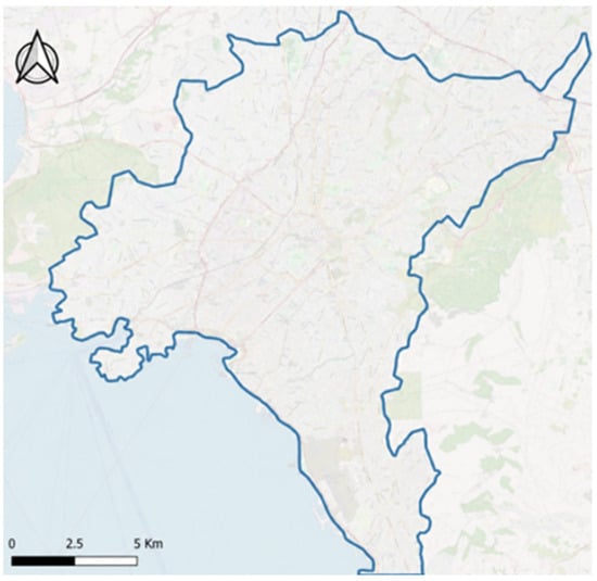
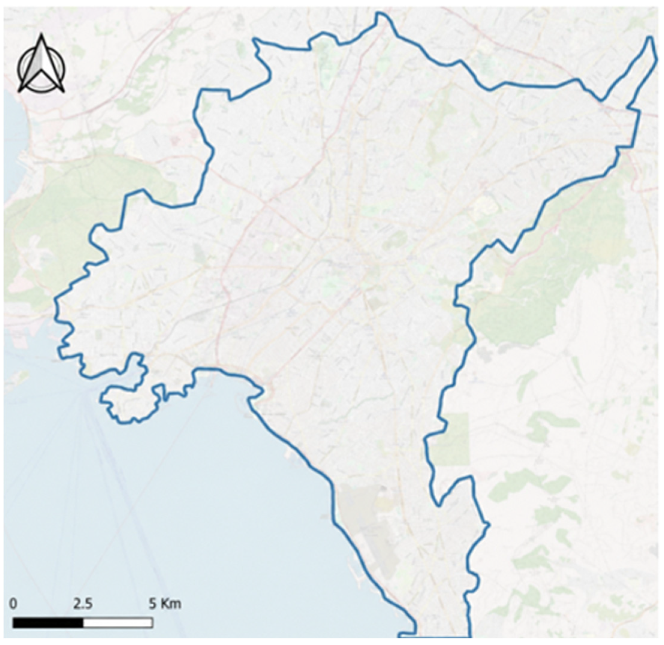
The study area covers the main continuous urban zone of the Attica Basin, from the southeastern coastal suburbs of Glyfada, Elliniko, and Alimos to Keratsini and Drapetsona in the southwest and the Attiki Odos motorway in the north (Figure 1). Mount Aigaleo and the Poikilo range bound the basin to the west, Mount Parnitha and Mount Penteli to the north, and Mount Hymettus to the east; the Saronic Gulf lies to the south. This setting produces clear gradients in elevation, exposure, maritime influence, urban development density, and vegetation cover.
Figure 1.
Location of the study area within the metropolitan Attica Basin. The blue outline delineates the boundary of the analyzed urban area.
2.2. Data and Preprocessing
Nine Landsat 8 Collection 1 Tier 1 images from 2020 were obtained from the USGS archive. The dataset included two winter images (28 January and 29 February), two spring images (17 April and 4 June), three summer images (22 July, 23 August, and 8 September), and two autumn images (late October and 27 November), with scene-level cloud cover below 10%. Images from March, May, and December were excluded due to cloud cover over 40%. Digital numbers were converted to top-of-atmosphere radiance or reflectance using scene-specific metadata coefficients, followed by dark-object subtraction of optical bands, per the source workflow and USGS guidance [19,20,21]. The input data and workflow are summarized in Table 1.
Table 1.
Input data and analytical workflow.
2.3. Estimation of NDVI and LST
NDVI was calculated for each image using OLI bands 5 (near-infrared) and 4 (red) as NDVI = (NIR − Red)/(NIR + Red). Values approaching +1 indicate dense photosynthetically active vegetation, whereas values near or below zero are typically associated with bare, built-up, or water surfaces. Seasonal NDVI layers were generated to characterize intra-annual variation in vegetation conditions.
LST estimation was based on TIRS band 10. Digital numbers were first converted to spectral radiance using L = M_L Q_cal + A_L, where M_L and A_L are the multiplicative and additive rescaling factors provided in the scene metadata. The satellite brightness temperature was then derived from the thermal calibration constants K1 and K2. The emissivity-correction procedure implemented in the original workflow was applied to convert brightness temperature to LST, and Kelvin values were converted to degrees Celsius by subtracting 273.15. Seasonal LST layers were generated from the available acquisitions and summarized by study unit. Because TIRS band 10 has a native spatial resolution of 100 m, the resulting temperatures were interpreted at the district and urban-zone scales.
2.4. Mapping the Composition and Structure of the Urban Landscape
Four high-resolution orthophoto mosaics with a ground sampling distance of 1.5 m were processed in eCognition Developer [11,22,23]. Multiresolution segmentation was used to create a homogeneous image-object layer. To achieve more appropriate object delineation, the scale parameter was set to 15 for most spatial units and to 20 for the larger spatial units.
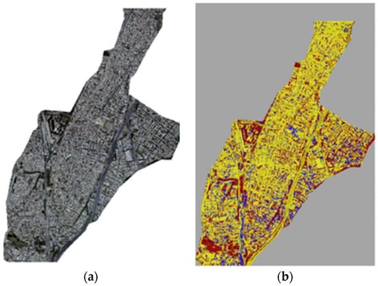
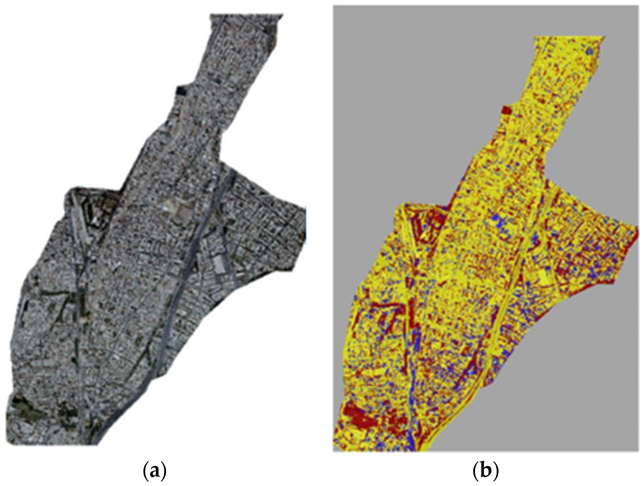
Classification rules combined object brightness, spectral ratios, spatial context, and a normalized red-green vegetation index. Three broad classes were mapped: vegetation/urban green space, built-up surfaces, and open/unbuilt land. This included formal green spaces such as parks, as well as smaller elements such as individual trees, planted courtyards, and roadside verges. The output was visually assessed and manually corrected where necessary to improve spatial and thematic accuracy. Hence, no formal accuracy assessment was conducted, and the classification was therefore used as a detailed explanatory layer rather than treated as a formally validated land-cover product (Figure 2).
Figure 2.
Land cover images: (a) representative orthophoto subset; (b) corresponding Object-Based Image Analysis (OBIA) classification showing vegetation (red), built-up area (yellow), and open/unbuilt surfaces (blue).
FRAGSTATS was used to describe urban landscape structure at class- and landscape-level [11,24]. Class-level metrics were the Number of Patches (NP), Percentage of Landscape (PLAND), Patch Density (PD), and area-weighted mean patch area. Landscape-level metrics were the Shannon and Simpson Diversity (SHDI and SIDI), Shannon evenness (SHEI), Mean Patch Size (MPS), Edge Density (ED), contagion (CON-TAG), Interspersion and Juxtaposition (IJI), and Landscape Shape Index (LSI). Mean elevation, east–west and north–south aspect components, terrain roughness, and distance from the sea were also estimated for each study unit.
2.5. Examining Seasonal LST–Landscape Structure Relationships
Seasonal and annual mean LST values were examined in relation to landscape metrics and topographic characteristics. Scatterplots and correlation matrices were first used to inspect bivariate relationships and identify strongly correlated predictors. Spatial and non-spatial regression models were then fitted for three predictor groups: vegetation-related landscape metrics, topographic variables, and a combined set. Backward elimination reduced the predictor set for each global multiple linear regression model, and a GWR model was fitted with the same predictors [10,11]. In addition, models were compared using R2 and AICc; lower AICc indicated a better balance of fit and complexity. Given the relatively small sample size (n = 30) and the absence of independent validation, the models were interpreted as explanatory rather than predictive.
3. Results
3.1. LST and NDVI Estimations
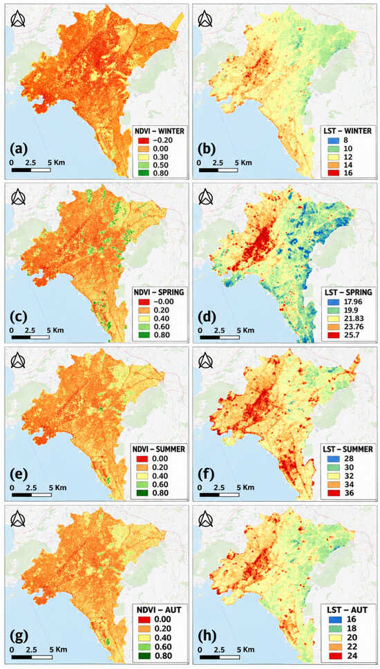
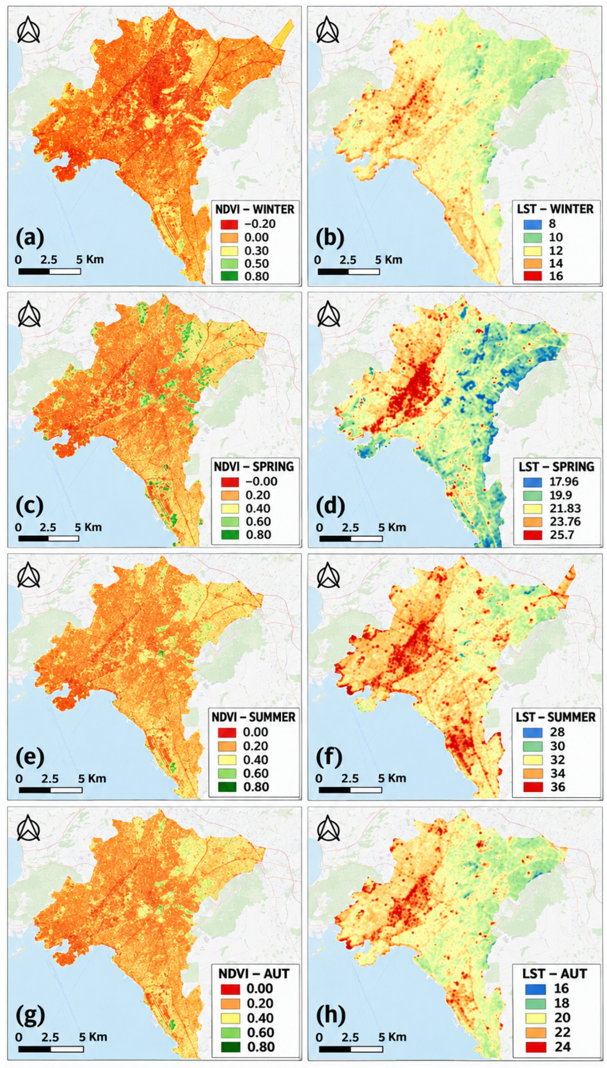
NDVI followed the expected seasonal cycle (Figure 3). Greenness was highest and most extensive in spring, particularly in the north, east, and around large parks, wooded hills, and stream corridors. In summer, high NDVI values were largely restricted to irrigated or densely vegetated areas. Winter and autumn NDVI were lower across most built-up districts. Areas with high NDVI repeatedly coincided with cooler surfaces in all four seasons (Figure 3).
Figure 3.
Seasonal spatial patterns of NDVI (left column) and LST (right column, °C) in 2020: (a,b) winter, (c,d) spring, (e,f) summer, and (g,h) autumn.
Seasonal LST maps showed a consistent thermal gradient (Figure 3). The central, western, and southwestern parts of the study area were generally warmer, especially around industrial zones and main roads and motorways. Cooler surfaces were concentrated in the northern and eastern regions of the basin, where elevation and vegetation cover are higher. Cooler areas were also observed around Lycabettus Hill, the National Garden, Attiko Alsos, Syngrou Forest, Pedion tou Areos, Nea Filadelfeia Grove, and vegetated stream corridors. Seasonal and annual LST ranges among the 30 study units are summarized in Table 2.
Table 2.
Seasonal and annual mean LST ranges among the study units.
Across the 30 study units, mean LST ranged from 9.51 to 13.18 °C in winter (range: 3.67 °C), 18.00 to 24.66 °C in spring (6.66 °C), 31.51 to 34.88 °C in summer (3.37 °C), and 21.08 to 24.48 °C in autumn (3.40 °C). Annual mean LST ranged from 20.39 to 24.30 °C. Agios Ioannis Rentis was the warmest unit in every seasonal and annual summary. The coolest unit varied by season: Agia Paraskevi in winter and annually, Alimos–Glyfada in spring, Filothei–Psychiko in summer, and Papagou–Cholargos in autumn. The wider range observed in spring, together with the seasonal shift in the coolest unit, highlights the combined influence of topography, coastal effects, vegetation phenology, and urban morphology on LST patterns.
Four contrasting settings were included in the point-based analysis: industrial/commercial surfaces, continuous dense development, discontinuous urban development, and urban green areas. LST declined monotonically as NDVI increased in every season. The fitted relationships were LST = 0.4534NDVI2 − 2.7919NDVI + 12.31 in winter (R2 = 0.8374), LST = −2.304ln(NDVI) + 20.792 in spring (R2 = 0.7524), LST = 27.431 × NDVI−0.103 in summer (R2 = 0.8112), and LST = 14.674NDVI2 − 18.419NDVI + 26.245 in autumn (R2 = 0.9118). Autumn produced the strongest fit and spring the weakest, although every model explained more than 75% of the sampled variation. Low-NDVI industrial and built surfaces were consistently warmer than densely vegetated samples.
3.2. Urban Landscape Composition and Structure
The classification results showed important differences among units. Mean vegetation cover was 20.80%, mean built-up cover was 74.60%, and mean open/unbuilt cover was 4.60%. PLAND_VEG ranged from 12.10% in Piraeus to 41.35% in Papagou–Cholargos. Other vegetation-rich units were Agia Paraskevi (37.11%), Chalandri (36.74%), Filothei–Psychiko (35.70%), and the fourth Athens sector (31.92%). At the other end of the range, Agios Ioannis Rentis (12.37%), Nikaia–Korydallos (12.60%), Kallithea (13.01%), and Peristeri (14.38%) had little vegetation. Built-up cover reached 84.41% in Dafni and exceeded 80% in several central and western units.
3.3. Relationship Between LST and Landscape Structure
District-scale relationships were weaker than point-scale NDVI–LST relationships, although their direction was consistent. The proportion of vegetated land (PLAND_VEG) was negatively associated with LST in every season, with R2 values of 0.437 in winter, 0.442 in spring, 0.528 in summer, and 0.384 in autumn. In summer, the fitted slope (−0.0761 °C per percentage point of vegetation) corresponds to about a 0.76 °C difference in mean LST for a 10-percentage-point difference in vegetation cover. This is an association, not a causal estimate. Built-up land (PLAND_B) showed the opposite pattern, with its strongest reported fit in spring (R2 approximately 0.46). Elevation was negatively associated with LST and had the strongest bivariate topographic fit in winter (R2 = 0.816).
The correlation matrices gave a similar picture. In winter, PLAND_VEG was negatively correlated with LST (r = −0.58), while PLAND_B was positively correlated (r = 0.47). The negative vegetation–LST correlation was stronger in summer (r = −0.67). Elevation had the strongest topographic association with LST, reaching r = −0.75 in summer. The east–west aspect component had the second strongest topographic association and was positively related to LST. Across the non-spatial analyses, vegetation proportion and elevation were the two most consistent negative covariates of surface temperature.
All GWR models had higher R2 values than their corresponding global models (Table 3). For vegetation-related metrics, GWR R2 ranged from 0.588 in autumn to 0.737 in spring. PLAND_VEG was retained in every seasonal and annual model, while CONTAG also entered the winter, spring, and annual models. Topographic models had the highest explanatory power, with R2 = 0.787 in winter and R2 = 0.752 for the annual mean. Elevation remained the main negative predictor, and the east–west aspect component was retained for autumn and the annual mean. The combined GWR models explained 73.8%, 74.6%, 73.2%, 71.1%, and 68.7% of LST variation in winter, spring, summer, autumn, and the annual mean, respectively. Allowing coefficients to vary spatially therefore raised R2, although the AICc comparison below also accounts for model complexity.
Table 3.
Comparison of global linear models and GWR by predictor group. R2, AICc, and retained predictors are reproduced from the source study.
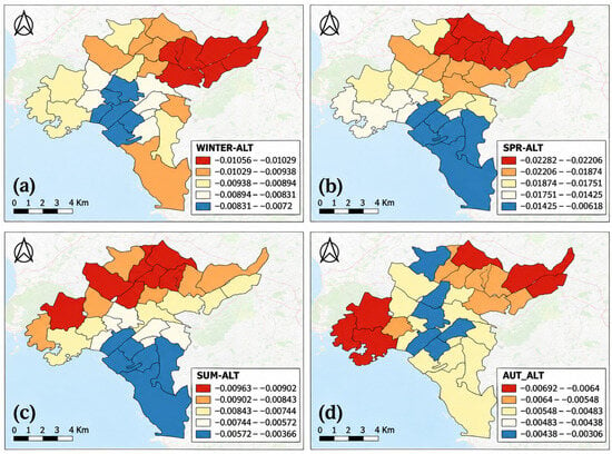
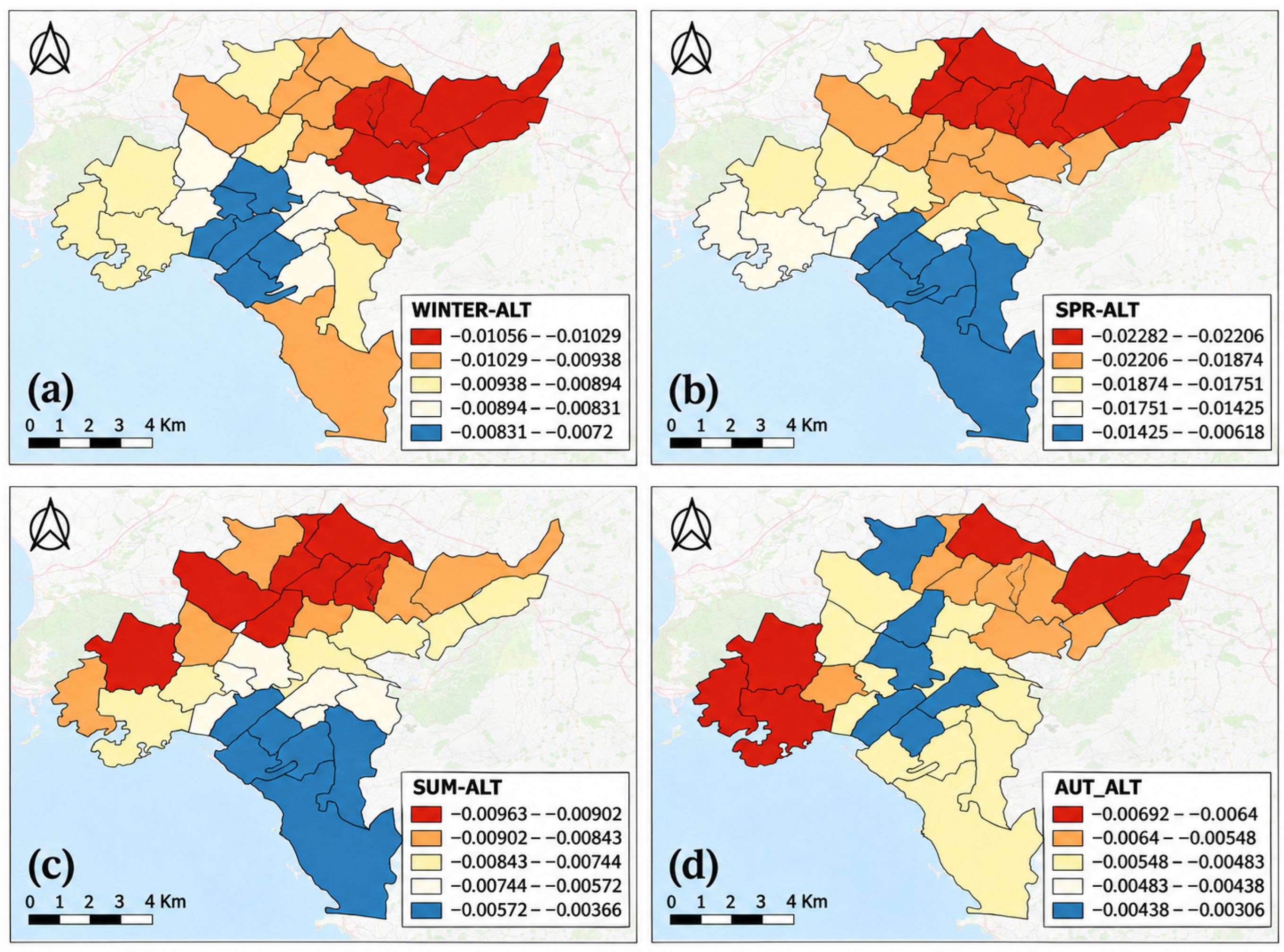
In all 15 comparisons, the GWR model had a higher AICc than its global counterpart, with ΔAICc values from 0.055 to 14.390. The spring vegetation and spring topographic models were nearly equivalent to the global models (ΔAICc < 0.1), and the spring combined model remained within 2 AICc units. In the other comparisons, the extra variance explained by GWR did not offset the added complexity. GWR is therefore more useful here for examining spatial non-stationarity than as a consistently better model. Elevation coefficients were negative throughout the study area in every season, but their magnitude varied in space and time (Figure 4).
Figure 4.
Seasonal GWR local coefficients for the elevation–LST relationship: (a) winter, (b) spring, (c) summer, and (d) autumn. All coefficients are negative; the mapped classes show spatial variation in coefficient magnitude.
4. Discussion
Understanding the vegetation–LST relationship requires more than demonstrating that greener areas are generally cooler. For urban thermal studies to provide robust and transferable evidence, it is important to determine how this relationship changes across seasons, spatial scales, landscape configurations, and topographic settings, as these factors can substantially affect both the magnitude and spatial pattern of the observed cooling effect. In this context, the well-established finding that greener surfaces tend to be cooler is not, by itself, the main contribution of this study. The added value lies in examining this relationship across four seasons, at both point and district scales, and within the pronounced topographic gradient of the Attica Basin. The contrast between the strong point-scale NDVI–LST relationships and the weaker district-scale PLAND_VEG–LST relationships demonstrates the sensitivity of the estimated association to the spatial unit of analysis. The models further distinguish the roles of vegetation amount, broader landscape configuration, and topography, while the combined use of R2 and AICc avoids interpreting the higher explanatory power of GWR as evidence of automatic model superiority. In this respect, the study complements earlier analyses of seasonal spatial non-stationarity [17] and previous Athens-based research focused on urban morphology and Local Climate Zones [18].
Warmer surfaces clustered in densely built-up districts, where vegetation is limited and industrial land uses and transport infrastructure are prominent. The greener, more elevated north and east part of the basin was generally cooler. Similar patterns have been reported in other Mediterranean cities, where urban form, relief, and coastal setting interact to create marked local temperature differences [12,13,14,15,16,18].
Vegetation was the most consistent land-cover correlate of lower LST. Both the point-scale NDVI analysis and the district-scale landscape analysis showed the same negative direction [2,3,4,5,6,7,9]. The stronger point-scale NDVI–LST fits, however, show why spatial resolution and analytical unit matter. NDVI describes the spectral condition of the sampled surface, whereas PLAND_VEG is the share of vegetation within a larger, internally mixed district. Parks, buildings, streets, open land, and other surfaces are combined within the same district value, weakening a local spectral–thermal relationship. Pixel- or sample-based cooling estimates should therefore not be transferred directly to planning districts without considering spatial aggregation and internal heterogeneity.
The results also suggest a role for landscape configuration, although the evidence is less direct than for vegetation amount. CONTAG was retained in several models, indicating that the aggregation and adjacency of land-cover classes may add information beyond total vegetation cover. Because CONTAG describes the entire landscape mosaic, it should not be read as a direct measure of green-space connectivity. Metrics designed specifically for vegetation patches would be needed to test whether connected, clustered, or dispersed green spaces differ in cooling performance [7,8,9].
The summer slope gives a useful sense of scale: a 10-percentage-point difference in vegetation was associated with about a 0.76 °C difference in mean LST. This estimate applies to municipal and submunicipal units. It does not mean that adding 10 percentage points of vegetation would cause the same amount of cooling. Vegetation also varies with elevation, building density, urban form, and other conditions that may contribute to the observed temperature difference.
Topography, especially elevation, was also central to the thermal pattern. Elevation was negatively associated with LST in every season and produced some of the strongest relationships in the analysis. The elevated north and east were generally cooler than the lower, more densely urbanized central and western districts. The east–west aspect component in selected models also suggests that terrain orientation changes solar exposure and interacts with the basin’s wider structure. Land cover alone therefore cannot explain surface-temperature variation in Athens; topographic attributes need to be considered.
Comparing the global models with GWR added important insights. GWR raised R2 in every predictor group and period, but its consistently higher AICc showed that the gain in explained variance rarely justified the additional complexity. Its clearest role in this study is diagnostic. Elevation coefficients stayed negative throughout the basin, yet their magnitude changed by location and season. This is useful evidence of spatial non-stationarity without implying that GWR is the better predictive model. For planning, the result argues against applying one vegetation target everywhere. Greening is likely to be most relevant in densely built, low-elevation, and thermally exposed districts, but its design should reflect local land cover, available space, topography, and distance from the coast [3,4,5,13,14,25].
Several limitations affect how far the results can be generalized. LST is the radiative temperature of the surface and is not equivalent to near-surface air temperature, human heat exposure, or outdoor thermal comfort [6,21]. The analysis also uses morning observations from nine cloud-screened images acquired in 2020. Its seasonal values are therefore a snapshot of that year, not climatological averages. Interannual differences in rainfall, vegetation condition, synoptic weather, and heat events could change both absolute LST and the strength of the fitted relationships. The stability of the relative spatial pattern should be tested with a longer time series. A further scale mismatch arises because the 100 m thermal data are compared with a 1.5 m land-cover map.
The spatial and thematic accuracy of the OBIA classification output was visually assessed and manually corrected; however, a quantitative classification accuracy assessment using an independent set of reference samples was not conducted. Misclassification among vegetation, built-up, and open/unbuilt surfaces, particularly in small, heterogeneous, or shaded patches, could therefore affect the estimated class proportions and derived landscape configuration metrics. Such errors may propagate into the district-level regression analyses and influence the magnitude and potentially the statistical significance of the estimated PLAND and CONTAG coefficients. Consequently, conclusions concerning the role of landscape composition and configuration should be interpreted with greater caution. By contrast, the point-scale NDVI–LST and elevation relationships are less affected by this limitation, as they are derived independently of the OBIA land-cover classes. Other constraints are the incomplete documentation of the emissivity correction, the small sample of 30 units, the absence of independent model validation, and the lack of an explicit test of residual spatial autocorrelation. These models should be read as explanatory rather than predictive.
A longer time series containing daytime and nighttime observations, ordinary summer days, and heat-wave periods would show whether the 2020 relationships persist. Comparing satellite LST with air-temperature or thermal-comfort measurements would also clarify their relevance to human exposure. Independent validation of the land-cover classification is needed before stronger conclusions can be drawn about configuration. More detailed data on green-space type, size, connectivity, and vegetation structure, together with analysis at several spatial scales, would help separate local cooling from broader district-level patterns [7,8,9].
5. Conclusions
Within the 2020 dataset, vegetation cover and elevation were the most consistent negative correlates of Land Surface Temperature (LST) across metropolitan Athens. Landscape configuration also contributed in some models, although this result is more sensitive to the unvalidated land cover map and should be treated cautiously. The large difference between point-scale Normalized Difference Vegetation Index (NDVI) fits and district-scale PLAND_VEG fits shows that estimated relationships depend on the analytical unit. GWR revealed spatial changes in coefficient strength, but the global models were more parsimonious. These findings favor locally adapted heat-mitigation strategies for densely built, low-elevation, and vegetation-poor districts, while also showing why vegetation targets should not be transferred unchanged across the Attica Basin.
Author Contributions
Conceptualization, G.S. and K.P.; methodology, G.S., G.K. and K.P.; software, formal analysis, data curation, and visualization, G.S.; validation, G.K. and K.P.; writing—original draft, G.S.; writing—review and editing, G.K. and K.P.; supervision, K.P. All authors have read and agreed to the published version of the manuscript.
Funding
This research received no external funding.
Institutional Review Board Statement
Not applicable.
Informed Consent Statement
Not applicable.
Data Availability Statement
Landsat data are available through USGS EarthExplorer; derived datasets are available from the corresponding author upon reasonable request.
Acknowledgments
ChatGPT 5.2 (OpenAI) was used for English-language editing and to improve selected parts of the text. The authors reviewed and revised the resulting text and take full responsibility for the final content of the manuscript.
Conflicts of Interest
The authors declare no conflicts of interest.
Abbreviations
The following abbreviations are used in this manuscript:
| LST | Land Surface Temperature |
| NDVI | Normalized Difference Vegetation Index |
| OBIA | Object-Based Image Analysis |
| PLAND | Percentage of Landscape |
References
- Tsiourlis, G.; Konstantinidis, P.; Xofis, P. Taxonomy and Ecology of Phryganic Communities with Sarcopoterium spinosum (L.) Spach of the Aegean (Greece). Isr. J. Plant Sci. 2007, 55, 15–34. [Google Scholar] [CrossRef] [Scilit]
- Dimoudi, A.; Nikolopoulou, M. Vegetation in the Urban Environment: Microclimatic Analysis and Benefits. Energy Build. 2003, 35, 69–76. [Google Scholar] [CrossRef] [Scilit]
- Chiesura, A. The Role of Urban Parks for the Sustainable City. Landsc. Urban Plan. 2004, 68, 129–138. [Google Scholar] [CrossRef] [Scilit]
- Baró, F.; Chaparro, L.; Gómez-Baggethun, E.; Langemeyer, J.; Nowak, D.J.; Terradas, J. Contribution of Ecosystem Services to Air Quality and Climate Change Mitigation Policies: The Case of Urban Forests in Barcelona, Spain. AMBIO 2014, 43, 466–479. [Google Scholar] [CrossRef] [Scilit] [PubMed]
- McPherson, E.G.; Simpson, J.R.; Peper, P.J.; Aguaron, E. Urban Forestry and Climate Change; USDA Forest Service: Albany, CA, USA, 2008.
- Weng, Q.; Lu, D.; Schubring, J. Estimation of Land Surface Temperature–Vegetation Abundance Relationship for Urban Heat Island Studies. Remote Sens. Environ. 2004, 89, 467–483. [Google Scholar] [CrossRef] [Scilit]
- Wang, X.; Cheng, H.; Xi, J.; Yang, G.; Zhao, Y. Relationship Between Park Composition, Vegetation Characteristics and Cool Island Effect. Sustainability 2018, 10, 587. [Google Scholar] [CrossRef] [Scilit]
- Flores, A.; Pickett, S.T.A.; Zipperer, W.C.; Pouyat, R.V.; Pirani, R. Adopting a Modern Ecological View of the Metropolitan Landscape: The Case of a Greenspace System for the New York City Region. Landsc. Urban Plan. 1998, 39, 295–308. [Google Scholar] [CrossRef] [Scilit]
- Kontogianni, A. The Impact of Urban Green Structure and Composition on the Climate of Cities. Ph.D. Thesis, Aristotle University of Thessaloniki, Thessaloniki, Greece, 2017. [Google Scholar]
- Fotheringham, A.S.; Brunsdon, C.; Charlton, M. Geographically Weighted Regression: The Analysis of Spatially Varying Relationships; Wiley: Chichester, UK, 2002. [Google Scholar]
- Kefalas, G. Spatiotemporal Analysis and Modeling of Landscape Changes and the Effects of Natural and Anthropogenic Factors. Ph.D. Thesis, Harokopio University, Kallithea, Greece, 2020. [Google Scholar]
- Giokas, K. The Urban Heat Island Phenomenon in Western Metropolitan Athens-Urban Planning Tools and Natural Mitigation Methods. Master’s Thesis, National Technical University of Athens, Athens, Greece, 2019. [Google Scholar]
- Kaloudis, S.; Kamperidis, G.; Polytscheris; Galanopoulou, S.; Lorentzos, N. Recreational Parks in the Urban Fabric of the Attica Basin. In Proceedings of the 2nd Conference on Geographic Information Systems and Spatial Analysis in Agriculture and the Environment; Agricultural University of Athens: Athens, Greece, 2017. [Google Scholar]
- Belavilas, N.; Vatavali, F.; Soureli, N.; Prentou, P. Open Spaces and Urban and Peri-Urban Green Areas in the Athens Metropolitan Complex. In Proceedings of the 3rd Panhellenic Conference on Urban Planning, Spatial Planning and Regional Development; University of Thessaly: Volos, Greece, 2012. [Google Scholar]
- Alcoforado, M.-J.; Andrade, H.; Lopes, A.; Vasconcelos, J. Application of Climatic Guidelines to Urban Planning. Landsc. Urban Plan. 2009, 90, 56–65. [Google Scholar] [CrossRef] [Scilit]
- Giannaros, T.M.; Melas, D. Study of the Urban Heat Island in a Coastal Mediterranean City: The Case Study of Thessaloniki, Greece. Atmos. Res. 2012, 118, 103–120. [Google Scholar] [CrossRef] [Scilit]
- Liu, H.; Zhan, Q.; Gao, S.; Yang, C. Seasonal Variation of the Spatially Non-Stationary Association Between Land Surface Temperature and Urban Landscape. Remote Sens. 2019, 11, 1016. [Google Scholar] [CrossRef] [Scilit]
- Agathangelidis, I.; Cartalis, C.; Santamouris, M. Urban Morphological Controls on Surface Thermal Dynamics: A Comparative Assessment of Major European Cities with a Focus on Athens, Greece. Climate 2020, 8, 131. [Google Scholar] [CrossRef] [Scilit]
- Roy, D.P.; Wulder, M.A.; Loveland, T.R.; Woodcock, C.E.; Allen, R.G.; Anderson, M.C.; Helder, D.; Irons, J.R.; Johnson, D.M.; Kennedy, R.; et al. Landsat-8: Science and Product Vision for Terrestrial Global Change Research. Remote Sens. Environ. 2014, 145, 154–172. [Google Scholar] [CrossRef] [Scilit]
- Landsat 8 (L8) Data Users Handbook; U.S. Geological Survey: Sioux Falls, SD, USA, 2019.
- Sekertekin, A.; Bonafoni, S. Land Surface Temperature Retrieval from Landsat 5, 7, and 8 over Rural Areas: Assessment of Different Retrieval Algorithms and Emissivity Models and Toolbox Implementation. Remote Sens. 2020, 12, 294. [Google Scholar] [CrossRef] [Scilit]
- Blaschke, T. Object Based Image Analysis for Remote Sensing. ISPRS J. Photogramm. Remote Sens. 2010, 65, 2–16. [Google Scholar] [CrossRef] [Scilit]
- Mallinis, G.; Gitas, I.Z.; Giannakopoulos, V.; Maris, F.; Tsakiri-Strati, M. An Object-Based Approach for Flood Area Delineation in a Transboundary Area Using ENVISAT ASAR and Landsat TM Data. Int. J. Digit. Earth 2013, 6, 124–136. [Google Scholar]
- McGarigal, K.; Cushman, S.A.; Ene, E. FRAGSTATS v4: Spatial Pattern Analysis Program for Categorical and Continuous Maps; University of Massachusetts: Amherst, MA, USA, 2012. [Google Scholar]
- Castán Broto, V.; Bulkeley, H. A Survey of Urban Climate Change Experiments in 100 Cities. Glob. Environ. Change 2013, 23, 92–102. [Google Scholar] [CrossRef] [Scilit] [PubMed]

Disclaimer/Publisher’s Note: The statements, opinions and data contained in all publications are solely those of the individual author(s) and contributor(s) and not of MDPI and/or the editor(s). MDPI and/or the editor(s) disclaim responsibility for any injury to people or property resulting from any ideas, methods, instructions or products referred to in the content. |
© 2026 by the authors. Licensee MDPI, Basel, Switzerland. This article is an open access article distributed under the terms and conditions of the Creative Commons Attribution (CC BY) license.