A Framework for Interactive Visualization and Evaluation of Classical Shortest-Path Algorithms in a Grid-Based Game ^†

Abstract

This paper presents the implementation and comparative evaluation of three classical shortest-path algorithms-Dijkstra, A*, and Bellman–Ford-within the Python/Pygame grid-based game environment PetWars. The developed framework provides a common environment for implementation, interactive visualization, and comparative benchmarking of the three algorithms under identical movement rules and map configurations. This common setup enables reproducible evaluation of path-finding behavior. The game models a 14 × 10 grid of walkable and blocked tiles, where movement is allowed in eight directions with weighted orthogonal and diagonal costs. The original PetWars map is used as an interactive demonstration environment. A dedicated demonstration mode visualizes the search process step by step by displaying the explored vertices, the frontier set, and the resulting shortest path. Performance is evaluated using five predefined routes and repeated measurements on two hardware configurations. Execution time, path cost, and the number of expanded vertices are analyzed under identical experimental conditions. The evaluated benchmark results agree with the theoretical characteristics of the evaluated algorithms. Within the implemented framework, A* explores fewer vertices and achieves the shortest execution times owing to heuristic guidance; Dijkstra examines a larger portion of the search space, whereas Bellman–Ford incurs the highest computational cost because of repeated edge relaxation. The developed application provides a common environment for benchmarking and visual demonstration of classical shortest-path algorithms.

1. Introduction

Shortest-path computation is a fundamental operation in graph-based planning and grid-based game environments. In a grid-based game, pathfinding affects how quickly a character reacts to a selected destination and how much of the map must be searched before a route is found.

Several families of algorithms are used for this purpose. Dijkstra’s algorithm [1] guarantees an optimal path in graphs with non-negative edge weights. A* [2] extends this approach by using a heuristic estimate to direct the search towards the target. Bellman–Ford [3,4] relies on repeated edge relaxation and can also process graphs with negative edge weights. Although the three algorithms are well established, their practical behavior depends on the graph structure, movement model, and implementation.

Previous studies examine pathfinding from different perspectives. Lawande et al. [5] review informed, uninformed, and metaheuristic methods used in video games. Duarte et al. [6] discuss pathfinding as a planning problem and relate algorithm selection to the characteristics of the search space and the available computation time. Comparative evaluations of classical and AI-based methods are reported by Aldhafferi [7]. Sapundzhi et al. [8] compare classical shortest-path algorithms on directed graphs. Here, the same algorithms are implemented and evaluated in the PetWars grid-based game environment, which also supports interactive visualization of the search process.

Research on grid-based environments also includes methods developed specifically for games, robotics, and navigation. Yap [9] examines grid-based pathfinding, while Lee and Lawrence [10] study fast pathfinding in video-game maps. Li et al. [11] examine the generation of alternative routes, and Kui and Yu [12] compare A*, Dijkstra, and Jump Point Search in complex terrain. Further modifications of A* and JPS have been proposed to reduce the explored area and improve search performance in particular grid configurations [13,14,15,16].

The present study integrates implementation, interactive visualization, application-level testing, and benchmarking in one Python 3.13/Pygame framework 2.6.1. Dijkstra, A*, and Bellman–Ford are implemented in the same graph representation and movement cost model. The original 14 × 10 PetWars map provides an illustrative game scenario.

The study examines whether the admissible octyl distance heuristic used by A* can reduce execution time and search-space exploration without increasing path cost. Dijkstra is used as the non-heuristic reference algorithm, whereas Bellman–Ford is a relaxation-based reference method. Several performance metrics are measured, including execution time, path cost, expanded vertices, edge relaxations, and speedup compared to Dijkstra’s method.

The remainder of the paper is organized as follows. Section 2 describes the algorithms, software implementation, and experimental methodology. Section 3 presents and discusses the experimental results. Section 4 summarizes the main conclusions and outlines directions for future work.

2. Materials and Methods

2.1. Shortest-Path Algorithms

Three classical shortest-path algorithms were selected for the experimental evaluation: Dijkstra’s algorithm [1], A* [2], and Bellman–Ford [3,4]. The algorithms represent different approaches to shortest-path computation while operating on the same graph representation. All three were implemented within the PetWars environment and evaluated using the same map, movement model, route set, and benchmarking procedure.

Dijkstra’s algorithm computes shortest paths in graphs with non-negative edge weights [4]. The implementation maintains tentative distances from the starting position and processes vertices in ascending order of distance using a priority queue. Let

$$G=(V, E),$$

(1)

where $V$ is the set of vertices and $E$ is the set of edges. Each edge $(u,v)$ has a non-negative weight $w(u,v)$, and the algorithm computes the minimum distance $d\left[v\right]$ from the source vertex to every reachable vertex. Using a binary heap, the implementation has a time complexity of $O\left(\left(V+E\right)\log V\right)$.

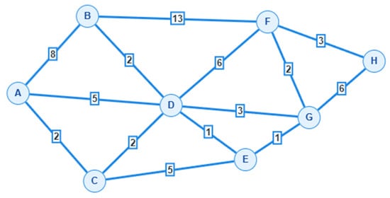
To illustrate the operation of the relaxation process, Dijkstra’s algorithm is used as an example. The weighted graph shown in Figure 1 demonstrates the network on which the successive distance updates are performed.

Figure 1. Example weighted undirected graph used to illustrate the relaxation process of Dijkstra’s algorithm.

The corresponding sequence of relaxation steps is presented in Table 1. The table shows how the tentative distances are updated after each iteration until the shortest path from the source vertex to all reachable vertices is established. The final shortest path from A to H has a total cost of 11 and follows the sequence A → C → D → E → G → F → H.

Table 1. Step-by-step relaxation when running Dijkstra’s algorithm from A to H.

V	A	B	C	D	E	F	G	H
A	0 ᴬ	8 ᴬ	2 ᴬ	5 ᴬ	∞	∞	∞	∞
C		8 ᴬ	2 ᴬ	4 E	7 E	∞	∞	∞
D		6 ᴰ		4 E	5 ᴰ	10 ᴰ	7 ᴰ	∞
E		6 ᴰ			5 ᴰ	10 ᴰ	6 ᴱ	∞
B		6 ᴰ				10 ᴰ	6 ᴱ	∞
G						8 G	6 ᴱ	12 G
F						8 G		11 F
H								11 F

Note: Superscript letters identify the predecessor vertex used to obtain each tentative distance. All vertex labels are written in uppercase.

A* extends Dijkstra’s algorithm by using a heuristic estimate of the remaining cost to the goal [5]. For each vertex n, the evaluation function is defined as

$$f\left(n\right)=g\left(n\right)+h\left(n\right),$$

(2)

where $g\left(n\right)$ is the accumulated cost from the start vertex to $n$, and $h\left(n\right)$ estimates the cost from $n$ to the goal.

The PetWars grid permits four orthogonal and four diagonal moves. Therefore, the implementation uses the octile-distance heuristic:

$$h\left(n\right) = D · max\left(\right|dx|, |dy\left|\right) + (D_2 - D) · min\left(\right|dx|, |dy\left|\right).$$

(3)

where $dx$ and $dy$ are the horizontal and vertical differences between the current vertex and the goal, $D$ is the cost of an orthogonal move, and $D_2$ is the cost of a diagonal move. In the implemented movement model, $D=2$ and $D_2=3$; thus, the heuristic becomes

$$h\left(n\right)=2 · max\left(\right|dx|, |dy\left|\right)+min\left(\right|dx|, |dy\left|\right).$$

(4)

The term $min(\left|dx\right|, \left|dy\right|)$ represents the number of diagonal moves that can be made towards the goal, whereas the difference between the two coordinate offsets corresponds to the remaining orthogonal moves. Since the heuristic uses the actual movement costs and does not overestimate the shortest possible remaining path, it is admissible for the adopted eight-direction movement model. A* therefore retains path optimality and can examine fewer vertices than Dijkstra’s algorithm.

Bellman–Ford computes shortest paths by repeatedly relaxing all graph edges [6,7]. During each iteration, every edge $(u, v)$ is examined. If the current distance estimate to vertex $v$ can be improved through vertex $u$,

$$d\left[u\right]+w\left(u, v\right)<d\left[v\right],$$

(5)

where $d\left[u\right]$ and $d\left[v\right]$ denote the current shortest distance estimates from the source vertex and $w(u, v)$ is the weight of the edge connecting them; the distance estimate is updated according to

$$d\left[u\right]+w(u, v).$$

(6)

The relaxation procedure is repeated $\mid V\mid -1$ times, where $\mid V\mid$ is the number of vertices in the graph. A final iteration checks whether any edge can still be relaxed, which would indicate a negative-weight cycle. To compare the computational efforts of three different search strategies under identical conditions, the Bellman–Ford method was included as a relaxation-based reference method.

Table 2 summarizes the computational complexity, main advantages, limitations, and role of the three algorithms in the present evaluation.

Table 2. Comparison of the three implemented algorithms.

Algorithm	Complexity	Advantages	Disadvantages
Dijkstra	$O\left(\right(V+E) log V)$	Optimal, reliable	Explores in all directions
A*	$O\left(\right(V+E) log V)$	Guided search, fast	Requires a good heuristic
Bellman–Ford	$O(V · E)$	Supports negative edge weights	Higher computational cost in the case of non-negative networks since the edges need to be relaxed several times.

2.2. Game Environment

The experimental evaluation was conducted in the PetWars game environment [17], which represents the game world as a two-dimensional grid. Each walkable cell is modeled as a graph vertex, whereas valid transitions between neighboring cells define the graph edges. Blocked cells are excluded from the graph and therefore cannot be traversed during pathfinding.

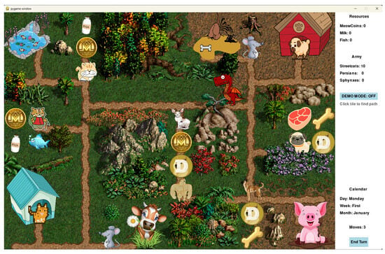
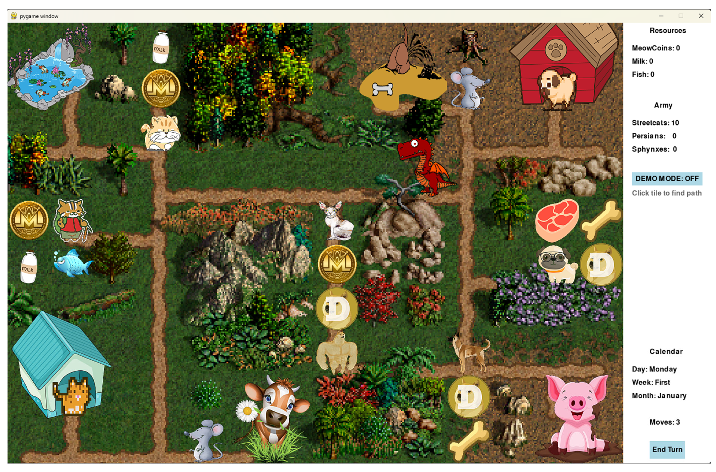
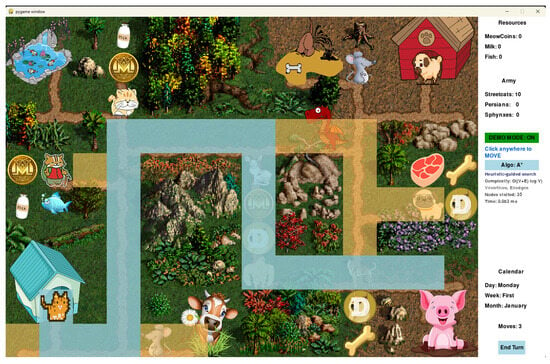
The game map consists of 14 × 10 cells, where each cell is classified as either walkable or blocked. The hero starts from a predefined position, and the destination is selected interactively by the user. Figure 2 shows the initial state of the game environment used throughout the experiments. The map should be used to visualize how pathfinding is integrated into the game interface to see the search process in real time.

Figure 2. Start screen of the game PetWars.

After the user selects a destination cell with a mouse click, the selected shortest-path algorithm computes the optimal route from the current hero position to the target. The computed path is then displayed on the game map, and the hero moves along the resulting route to the selected destination.

Three pathfinding-related features were added to the original game engine: a movement-point system, eight-direction movement, and smooth path rendering based on Chaikin’s corner-cutting algorithm [18]. The hero has 10 movement points per turn, with orthogonal and diagonal moves requiring 2 and 3 points, respectively. These extensions support the integration and visualization of the evaluated pathfinding algorithms within the game environment.

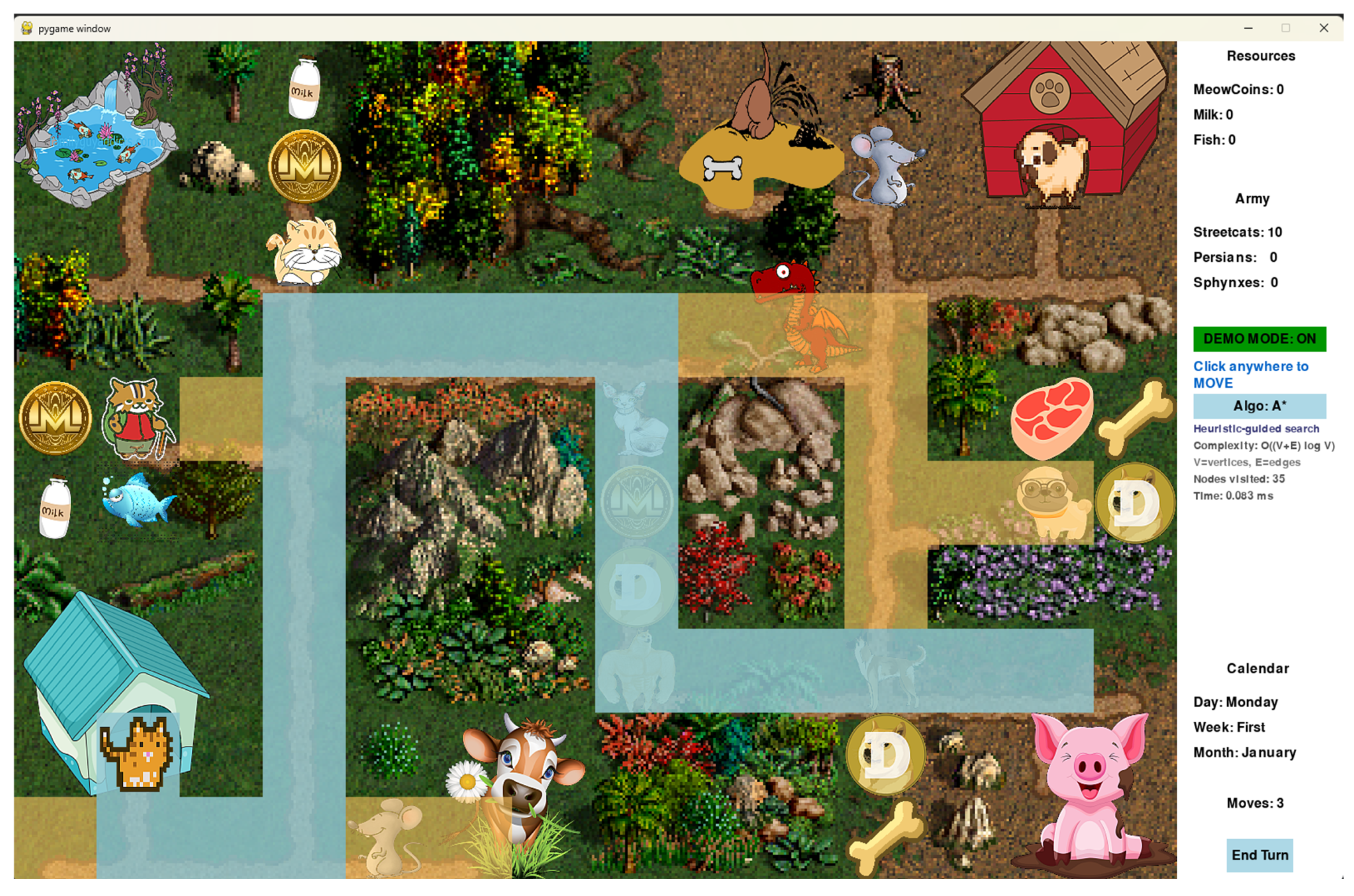
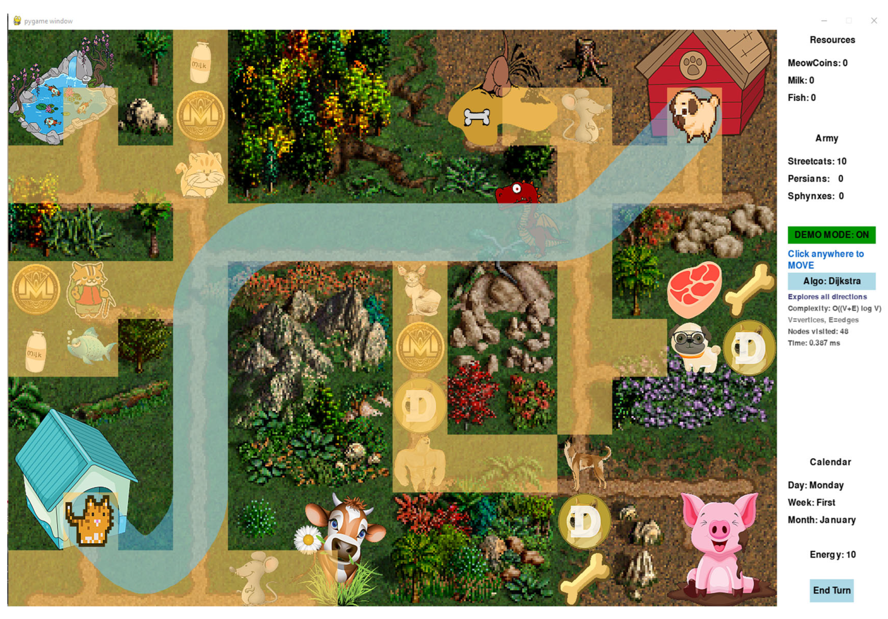
In addition to normal gameplay, the application provides a demonstration mode for visualizing the search process. Visited vertices are shown in orange, frontier vertices in yellow, the currently expanded vertex in red, and the final shortest path in blue. Demo mode is activated through the corresponding interface button or by pressing the D key, and the visualization proceeds step by step with an adjustable delay. Figure 3 illustrates the visual representation of the search process.

Figure 3. Demo-mode visualization of the explored cells, frontier cells, and the final computed path.

2.3. Software Implementation

The experimental framework was implemented in Python using the Pygame library for the graphical interface. The full source code is publicly available at https://github.com/hristogwivanov/PetWars (accessed on 1 November 2026). The application is organized into separate modules responsible for the game loop, pathfinding algorithms, game data, configuration parameters, and user interface components.

The main modules are

• main.py—manages the game loop and rendering;
• pathfinding.py—contains the implementations of Dijkstra’s, A*, and Bellman–Ford algorithms;
• gamedata.py—defines the classes for heroes, resources, and the AI opponent;
• constants.py—stores constants, colors, and terrain maps;
• interface.py—provides the user interface components, including buttons and the turn counter.

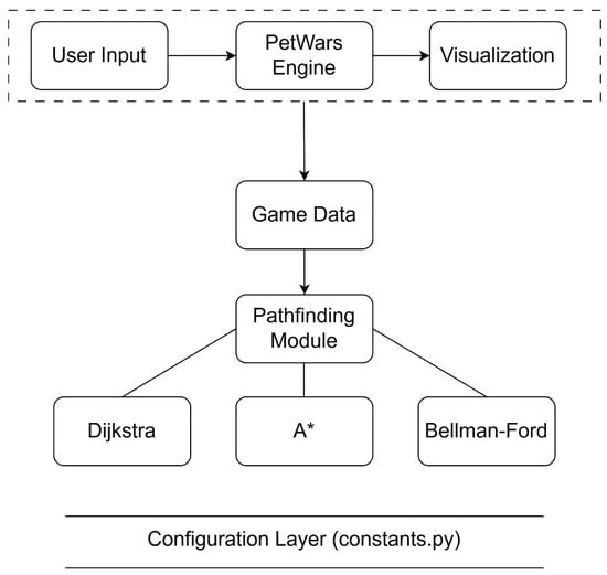
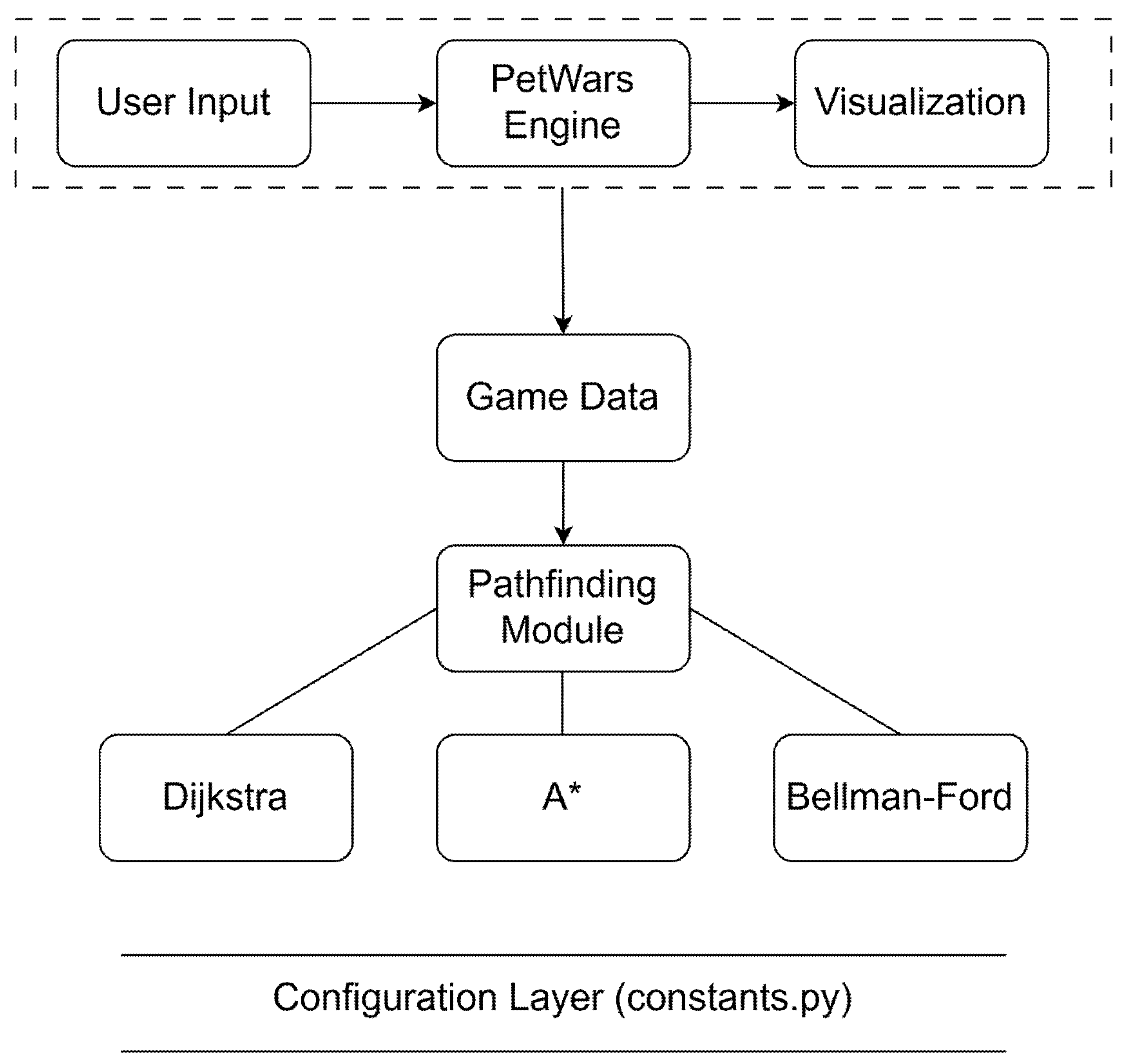
Figure 4 presents the software architecture of the PetWars application. The game engine processes user input, updates the game state, and controls rendering. Game data are forwarded to the pathfinding module, which executes the selected shortest-path algorithm and returns the computed route to the game engine for visualization and character movement.

Figure 4. Software architecture of the PetWars application.

The implementation details of the three shortest-path algorithms are summarized below. Dijkstra’s algorithm was implemented using a priority queue and non-negative movement costs. Vertices are processed in ascending order of their current distance from the starting position. In the PetWars environment, orthogonal and diagonal movements have costs of 2 and 3, respectively. The main implementation steps are summarized in Algorithm 1.

Algorithm 1: Dijkstra’s Algorithm
Data: grid map, start cell, goal cell
Result: shortest path and its cost
Initialize: dist[start] ← 0, all others ← ∞;
insert (0, start) into priority queue Q;
while Q is not empty do
	(d, u) ← extract vertex with minimum distance from Q;
	if u = goal then return path and cost;
	if d > dist[u] then continue;
	foreach neighbour v of u (4 orthogonal + 4 diagonal) do
		cost ← weight(u, v) (2 orthogonal, 3 diagonal);
		if dist[u] + cost < dist[v] then
			dist[v] ← dist[u] + cost;
			prev[v] ← u;
			insert (dist[v], v) into Q;
		end
	end
end
return “no path”;

The A* implementation uses the same grid representation and movement costs as Dijkstra’s algorithm. The search is guided by the octile-distance heuristic defined in Equation (4). The principal implementation steps are presented in Algorithm 2.

Algorithm 2: A* Algorithm (octile heuristic)
Data: grid map, start cell, goal cell
Result: shortest path and its cost
Initialize: g[start] ← 0, all others ← ∞;
h(n) ← 2 · max(|dx|, |dy|) + min(|dx|, |dy|) (octile, D = 2, D2 = 3);
insert (h(start), start) into priority queue Q;
while Q is not empty do
	u ← vertex in Q with minimum f = g + h;
	if u = goal then return path and cost;
	if u is visited then continue;
	mark u as visited;
	foreach neighbour v of u (4 orthogonal + 4 diagonal) do
		if v is visited then continue;
		cost ← weight(u, v) (2 orthogonal, 3 diagonal);
		if g[u] + cost < g[v] then
			g[v] ← g[u] + cost;
			prev[v] ← u;
			insert (g[v] + h(v), v) into Q;
		end
	end
end
return “no path”;

The Bellman–Ford implementation constructs an edge list from the walkable cells and applies repeated edge relaxation using the same orthogonal and diagonal movement costs as the other algorithms. The implementation includes early termination when an iteration produces no distance updates. Its principal steps are summarized in Algorithm 3.

Algorithm 3: Bellman–Ford Algorithm
Data: grid map, start cell, goal cell
Result: shortest path and its cost
Initialize: dist[start] ← 0, all others ← ∞;
build edge list E over walkable cells (cost 2 orthogonal, 3 diagonal);
for i ← 1 to |V| − 1 or until no changes do
	foreach edge (u, v) in E do
		if dist[u] + weight(u, v) < dist[v] then
			dist[v] ← dist[u] + weight(u, v);
			prev[v] ← u;
		end
	end
end
if dist[goal] = ∞ then return “no path”;
return path and cost;

2.4. Experimental Procedure

The performance of Dijkstra’s, A*, and Bellman–Ford was evaluated with the original PetWars game environment. During each experiment, one of the three algorithms was selected through the graphical interface, and a destination cell was specified on the game map. The algorithm calculated the shortest path from the current position of the hero to the selected destination, after which the movement was visualized in the game environment.

For each hardware platform, the algorithms were run on the same map, with the same movement rules, and the same start and destination positions. There were differences in operating system and Python version, so the runtimes are reported descriptively and should not be used to conclude differences between processors.

Five representative routes with different lengths and obstacle distributions were selected for benchmarking. Each route was executed independently with all three algorithms. For every combination of route, algorithm, and hardware platform, the execution-time measurement was repeated 30 times. The reported statistics include the minimum, mean, maximum, and standard deviation of the recorded execution times.

The benchmarking experiments were performed on two hardware platforms with different performance characteristics. The hardware and software configurations of both test platforms are summarized in Table 3.

Table 3. Hardware and software configurations used for the benchmarks.

Component	Ryzen 5 3400G	Ryzen 9 5900X
CPU cores/base clock	4 cores, 3.7–4.2 GHz	12 cores, 3.7–4.8 GHz
CPU Cache	6 MB	70 MB
CPU TDP	65 W	105 W
Memory	16 GB DDR4-3200, dual channel	32 GB DDR4-3200, dual channel
Graphics	Integrated Radeon Vega 11	GeForce RTX 3060 Ti 8 GB
Operating system	Windows 10	Windows 11
Python	3.13.3	3.11.9
Pygame	2.6.1	2.6.1

The execution time of each algorithm was measured using the same benchmarking procedure. For every combination of route, algorithm, and hardware platform, one warm-up execution was performed and excluded from the reported results. This was followed by 30 independent timed executions using the high-resolution perf_counter() function. The minimum, mean, maximum, and standard deviation of the recorded execution times were calculated. The complete measurement procedure is summarized in Algorithm 4.

Algorithm 4: Execution-time measurement
Data: grid map G, start cell s, goal cell t, pathfinding algorithm A, number of repetitions N
Result: minimum, mean, maximum, and standard deviation of execution time
times ← empty list
Perform one warm-up execution: A(G, s, t)
for i ← 1 to N do
	start_time ← perf_counter() A(G, s, t) end_time ← perf_counter()
	elapsed_time ← (end_time − start_time) × 1000 append elapsed_time to times
end
minimum_time ← min(times) mean_time ← mean(times) maximum_time ← max(times) standard_deviation ← std(times) return minimum_time, mean_time, maximum_time, standard_deviation

3. Results and Discussion

3.1. Qualitative Results

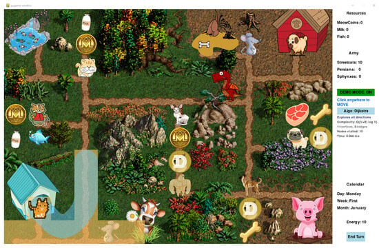
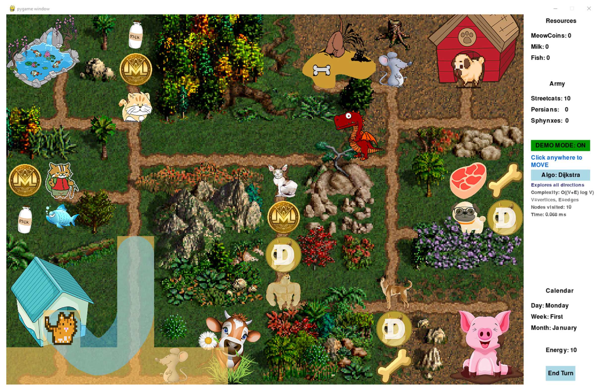
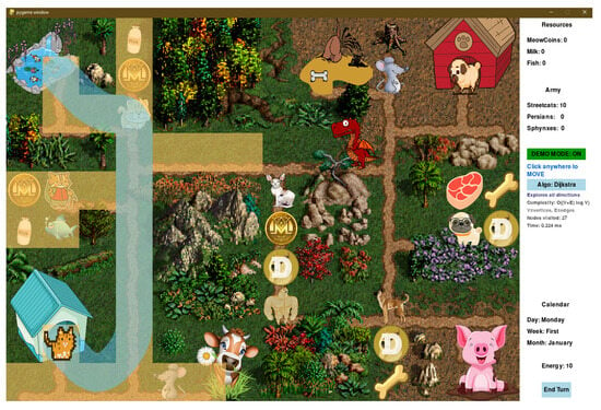
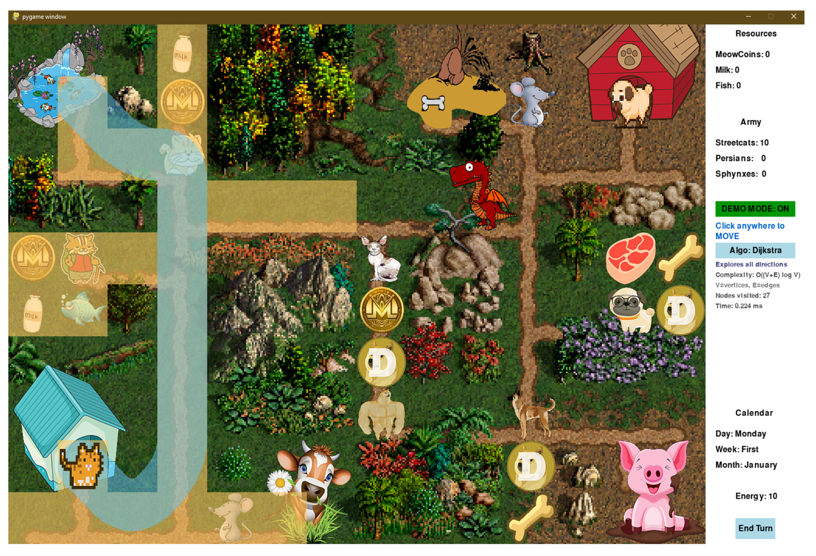
Three representative routes were selected to demonstrate the behavior of the implemented pathfinding algorithms under different traversal distances. The selected scenarios correspond to short-, medium-, and long-distance routes measured from the same starting position. Figure 5, Figure 6 and Figure 7 show the paths generated by Dijkstra’s algorithm for the three scenarios.

Figure 5. Dijkstra’s algorithm at a short distance.

Figure 6. Dijkstra’s algorithm at a medium distance.

Figure 7. Dijkstra’s algorithm at a long distance.

The short-distance route extends from the starting position (1, 8) to the target cell (3, 3), with a path length of 16. As shown in Figure 5, the destination is reached after exploring only a small part of the map.

The medium-distance route extends from (1, 8) to (10, 2), with a path length of 30. Compared with the previous scenario, the search covers a larger area before the destination is reached (Figure 6).

The long-distance route extends from (1, 8) to (13, 4), with a path length of 38. Figure 7 shows that the explored area increases further as the route becomes longer.

3.2. Results on the Original PetWars Map

Five test routes were used to compare the performance of the implemented algorithms. Table 4 summarizes the path length and the number of visited (expanded) vertices for each route. The number of expanded nodes and the path cost depend on the map, the origin-destination pair, the traffic rules, and the algorithm’s implementation, not on the hardware. Table 5 and Table 6 present the execution-time statistics obtained on the two experimental systems.

Table 4. Test routes and number of visited (expanded) vertices per algorithm. Visited counts are hardware-independent.

Scenario	Start → Goal	Path Cost	Dijkstra	A*
Short distance	(1, 8) → (3, 3)	16	14	9
Medium distance	(1, 8) → (10, 2)	30	37	19
Long distance	(1, 8) → (13, 4)	38	56	28
Random 1	(10, 9) → (3, 3)	25	35	15
Random 2	(13, 5) → (0, 2)	29	47	14

Table 5. Execution-time statistics on the AMD Ryzen 5 3400G, in milliseconds (30 repetitions per route/algorithm). Speed-up is relative to Dijkstra on the same route.

Scenario	Algorithm	Min	Mean	Max	Std	Speed-Up
Short distance	Bellman–Ford	0.6513	0.7824	1.0782	0.1499	0.17×
Short distance	Dijkstra	0.0807	0.1292	0.3113	0.0544	1.00×
Short distance	A*	0.0635	0.0856	0.1296	0.0183	1.51×
Medium distance	Bellman–Ford	0.6507	0.7980	1.7552	0.2417	0.29×
Medium distance	Dijkstra	0.2225	0.2278	0.2449	0.0063	1.00×
Medium distance	A*	0.1359	0.1770	0.3153	0.0547	1.29×
Long distance	Bellman–Ford	0.6663	1.0364	1.5924	0.2231	0.38×
Long distance	Dijkstra	0.3408	0.3960	0.7385	0.0907	1.00×
Long distance	A*	0.2147	0.2548	0.3520	0.0492	1.55×
Random 1	Bellman–Ford	0.8254	0.9607	1.5022	0.1710	0.29×
Random 1	Dijkstra	0.2126	0.2811	0.3472	0.0231	1.00×
Random 1	A*	0.1105	0.1541	0.3551	0.0439	1.82×
Random 2	Bellman–Ford	0.7092	0.7809	0.9234	0.0607	0.47×
Random 2	Dijkstra	0.2965	0.3689	0.5108	0.0611	1.00×
Random 2	A*	0.1185	0.1496	0.2038	0.0251	2.47×

Table 6. Execution-time statistics on the AMD Ryzen 9 5900X, in milliseconds (30 repetitions per route/algorithm). Speed-up is relative to Dijkstra on the same route.

Scenario	Algorithm	Min	Mean	Max	Std	Speed-Up
Short distance	Bellman–Ford	0.2293	0.2364	0.2610	0.0064	0.14×
Short distance	Dijkstra	0.0262	0.0323	0.0409	0.0043	1.00×
Short distance	A*	0.0237	0.0284	0.0530	0.0069	1.14×
Medium distance	Bellman–Ford	0.2304	0.2574	0.4648	0.0586	0.29×
Medium distance	Dijkstra	0.0718	0.0741	0.0816	0.0028	1.00×
Medium distance	A*	0.0485	0.0495	0.0551	0.0013	1.50×
Long distance	Bellman–Ford	0.2322	0.2539	0.3119	0.0260	0.47×
Long distance	Dijkstra	0.1140	0.1203	0.1544	0.0099	1.00×
Long distance	A*	0.0775	0.0880	0.1257	0.0133	1.37×
Random 1	Bellman–Ford	0.2969	0.3148	0.3869	0.0236	0.23×
Random 1	Dijkstra	0.0700	0.0724	0.0855	0.0033	1.00×
Random 1	A*	0.0369	0.0407	0.0696	0.0078	1.78×
Random 2	Bellman–Ford	0.2749	0.3263	0.5592	0.0863	0.45×
Random 2	Dijkstra	0.0964	0.1481	0.3082	0.0471	1.00×
Random 2	A*	0.0419	0.0447	0.0545	0.0031	3.31×

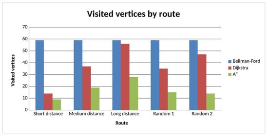
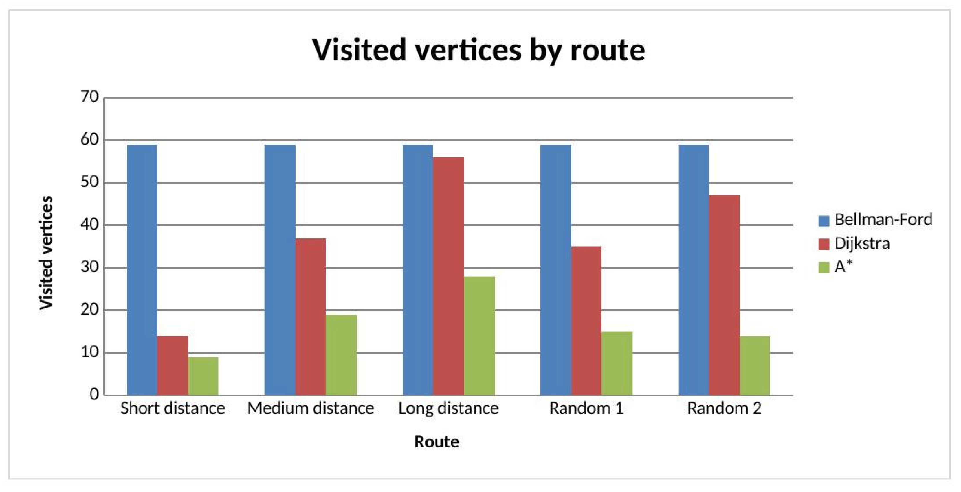
All three algorithms produced identical shortest-path costs for every evaluated route. Table 4 shows that A* expands fewer vertices than Dijkstra for all evaluated routes, ranging from 9 to 28 vertices compared with 14 to 56 vertices for Dijkstra. This corresponds to reductions of approximately 36% to 70%. Expanded-vertex counts are not reported for Bellman–Ford because its repeated edge relaxation procedure does not follow the same node-expansion paradigm as Dijkstra and A*. Its computational cost is therefore assessed through execution time. The lower expanded-vertex counts achieved by A* are generally consistent with execution-time measurements reported in Table 5 and Table 6.

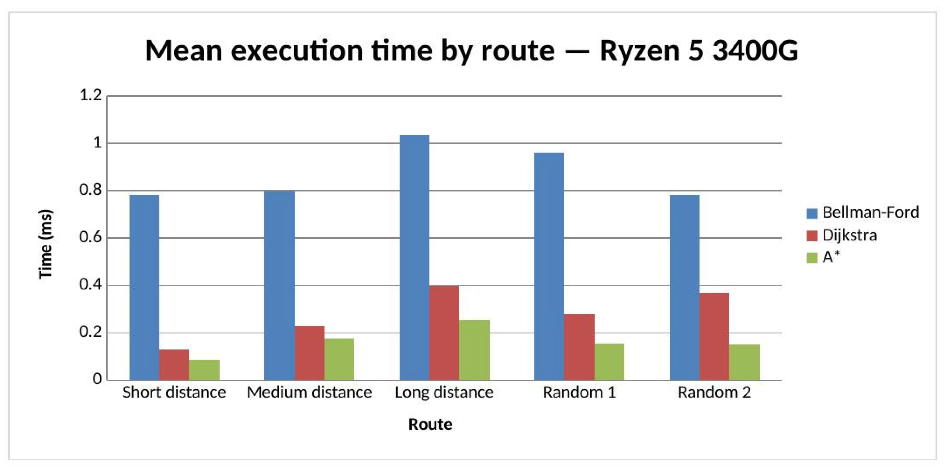
The results of the execution time on the AMD Ryzen 5 3400G processor demonstrate the same trend as the extended vertex counts. First, A* has the shortest average execution time for all the routes, followed by Dijkstra, with Bellman–Ford having the longest execution time. Thus, the speed-up of A* compared to Dijkstra is in the range of 1.29-2.47x. Compared to Dijkstra, most of the execution time measurements have a considerable variance, likely due to the values being in the sub-millisecond range for the original graph. The results should be considered in the context of implementation specifics rather than general algorithmic efficiency.

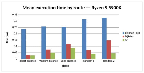
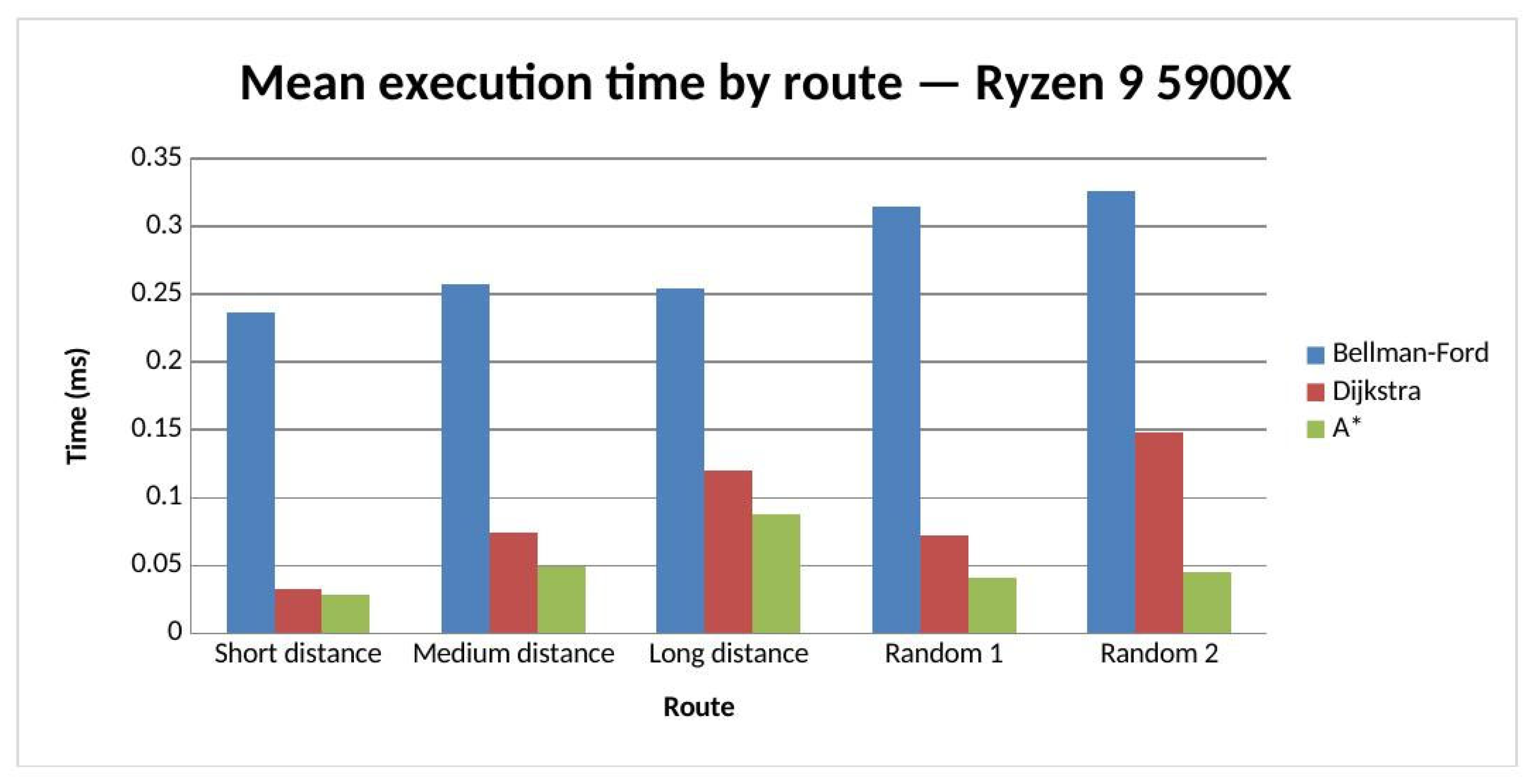
The measurements obtained on the AMD Ryzen 9 5900X follow the same performance ranking observed on the AMD Ryzen 5 3400G. A* again achieves the shortest execution times for all evaluated routes, followed by Dijkstra, while Bellman–Ford remains the slowest algorithm. The performance improvement of A* over Dijkstra ranges from 1.14× to 3.31× across the evaluated routes. Across the 30 benchmark runs, the standard deviations were mostly low in absolute terms, suggesting stable runtimes of these implementations on each particular setup. However, as the benchmarked runtimes were below a millisecond, the results primarily reflect implementation-level differences rather than algorithm-level performance.

Identical quality rankings were obtained on both test platforms. However, due to differences in processors, not only the Python version software components but also the characteristics of the computers on which the calculations were performed, such as memory and cache, were different. The second platform was used only to check whether the result obtained was not affected by these differences.

Figure 8, Figure 9 and Figure 10 present the benchmark results graphically for the evaluated algorithms.

Figure 8. Mean execution time by route on the Ryzen 5 3400G.

Figure 9. Mean execution time by route on the Ryzen 9 5900X.

Figure 10. Number of visited (expanded) vertices by route (identical on both machines).

The visualizations confirm the trends identified in the quantitative analysis and highlight the correspondence between execution time and the number of expanded vertices across the evaluated routes.

3.3. Discussion

The experimental evaluation reveals consistent differences in the performance of the three evaluated shortest-path algorithms. For all test routes, A* achieves the shortest execution time, followed by Dijkstra, whereas Bellman–Ford requires the longest computation time. The same ranking is observed on both evaluated hardware platforms, indicating that the relative performance of the algorithms is independent of the computing platform.

The performance differences can be explained by the search strategy employed by each algorithm. By using the octile-distance heuristic, A* directs the search towards the destination and explores fewer vertices while preserving path optimality. Dijkstra also guarantees an optimal solution but performs an uninformed search, which results in a larger search space and longer execution times. In contrast, Bellman–Ford repeatedly relaxes all graph edges regardless of the destination location, leading to the highest computational cost in the evaluated game environment. Route length influences execution time indirectly by increasing the size of the explored search region. Consequently, algorithms that restrict the number of expanded vertices achieve lower execution times.

The experimental observations agree with the expected theoretical behavior of the evaluated algorithms. In grid-based environments with non-negative movement costs, heuristic search reduces the number of explored vertices without affecting the optimality of the computed path. Under the same conditions, Dijkstra remains an effective solution when no heuristic information is available. Bellman–Ford, although applicable to a wider class of graph problems, offers no practical performance advantage in the considered environment because support for negative edge weights is not required.

The present study has several limitations. The experiments were performed on a single static game map with predefined obstacles and uniform movement costs using a fixed set of benchmark routes. Only three classical shortest-path algorithms were included in the comparison. Furthermore, the evaluation focused on execution time and the number of expanded vertices. Other performance characteristics, such as memory consumption, scalability to substantially larger environments, and behavior in dynamic game scenarios with changing obstacles, were not investigated.

4. Conclusions

Three classical shortest-path algorithms—Dijkstra, A*, and Bellman–Ford were implemented and evaluated within the PetWars game environment under identical movement rules, map configuration, and benchmarking conditions. The developed implementation also supports step-by-step visualization of the search process, making the behavior of the algorithms directly observable.

The experimental results show that all three algorithms return shortest paths of identical length for the evaluated routes. Their computational performance differs considerably. A* achieves the lowest execution times and expands the fewest vertices, Dijkstra requires a larger search space, and Bellman–Ford is the least efficient algorithm in the tested environment. The same ranking is observed on both hardware platforms.

In the evaluated game environment, A* achieves the shortest execution times and expands the fewest vertices. Dijkstra remains a suitable alternative when heuristic information is unavailable, whereas Bellman–Ford is more appropriate for applications that require support for negative edge weights.

Future work will include experiments on larger maps, dynamic environments, and additional pathfinding algorithms, including Jump Point Search and Theta*, to extend the comparative evaluation.

References

- Dijkstra, E.W. A Note on Two Problems in Connexion with Graphs. Numer. Math. 1959, 1, 269–271. [Google Scholar] [CrossRef] [Scilit]
- Hart, P.; Nilsson, N.; Raphael, B. A Formal Basis for the Heuristic Determination of Minimum Cost Paths. IEEE Trans. Syst. Sci. Cyber. 1968, 4, 100–107. [Google Scholar] [CrossRef] [Scilit]
- Bellman, R. On a Routing Problem. Quart. Appl. Math. 1958, 16, 87–90. [Google Scholar] [CrossRef] [Scilit]
- Ford, L.R. Network Flow Theory. In Linear Programming; Springer Series in Operations Research and Financial Engineering; Springer: New York, NY, USA, 1997; pp. 253–313. [Google Scholar] [CrossRef] [Scilit]
- Lawande, S.R.; Jasmine, G.; Anbarasi, J.; Izhar, L.I. A Systematic Review and Analysis of Intelligence-Based Pathfinding Algorithms in the Field of Video Games. Appl. Sci. 2022, 12, 5499. [Google Scholar] [CrossRef] [Scilit]
- Duarte, F.F.; Lau, N.; Pereira, A.; Reis, L.P. A Survey of Planning and Learning in Games. Appl. Sci. 2020, 10, 4529. [Google Scholar] [CrossRef] [Scilit]
- Aldhafferi, N. Time and Memory Trade-Offs in Shortest-Path Algorithms Across Graph Topologies: A*, Bellman–Ford, Dijkstra, AI-Augmented A* and a Neural Baseline. Computers 2025, 14, 545. [Google Scholar] [CrossRef] [Scilit]
- Sapundzhi, F.; Danev, K.; Ivanova, A.; Popstoilov, M.; Georgiev, S. A Performance Comparison of Shortest Path Algorithms in Directed Graphs. Eng. Proc. 2025, 100, 31. [Google Scholar] [CrossRef] [Scilit]
- Yap, P. Grid-Based Path-Finding. In Advances in Artificial Intelligence; Cohen, R., Spencer, B., Eds.; Lecture Notes in Computer Science; Springer: Berlin/Heidelberg, Germany, 2002; Volume 2338, pp. 44–55. [Google Scholar] [CrossRef] [Scilit] [PubMed]
- Lee, W.; Lawrence, R. Fast Grid-Based Path Finding for Video Games. In Advances in Artificial Intelligence; Zaïane, O.R., Zilles, S., Eds.; Lecture Notes in Computer Science; Springer: Berlin/Heidelberg, Germany, 2013; Volume 7884, pp. 100–111. [Google Scholar] [CrossRef] [Scilit]
- Li, L.; Cheema, M.A.; Ali, M.E.; Lu, H.; Li, H. Efficiently Computing Alternative Paths in Game Maps. World Wide Web 2023, 26, 3321–3345. [Google Scholar] [CrossRef] [Scilit]
- Kui, L.; Yu, X. A Pathfinding Algorithm for Large-Scale Complex Terrain Environments in the Field. IJGI 2024, 13, 251. [Google Scholar] [CrossRef] [Scilit]
- Ou, Y.; Fan, Y.; Zhang, X.; Lin, Y.; Yang, W. Improved A* Path Planning Method Based on the Grid Map. Sensors 2022, 22, 6198. [Google Scholar] [CrossRef] [Scilit] [PubMed]
- Gong, H.; Tan, X.; Wu, Q.; Li, J.; Chu, Y.; Jiang, A.; Han, H.; Zhang, K. Bidirectional Jump Point Search Path-Planning Algorithm Based on Electricity-Guided Navigation Behavior of Electric Eels and Map Preprocessing. Biomimetics 2023, 8, 387. [Google Scholar] [CrossRef] [Scilit] [PubMed]
- Luo, Y.; Lu, J.; Qin, Q.; Liu, Y. Improved JPS Path Optimization for Mobile Robots Based on Angle-Propagation Theta* Algorithm. Algorithms 2022, 15, 198. [Google Scholar] [CrossRef] [Scilit]
- Wang, F.; Sun, W.; Yan, P.; Wei, H.; Lu, H. Research on Path Planning for Robots with Improved A* Algorithm under Bidirectional JPS Strategy. Appl. Sci. 2024, 14, 5622. [Google Scholar] [CrossRef] [Scilit]
- Ivanov, H.N. PetWars, 2026. Available online: https://github.com/hristogwivanov/PetWars (accessed on 1 November 2026).
- Chaikin, G.M. An Algorithm for High-Speed Curve Generation. Comput. Graph. Image Process. 1974, 3, 346–349. [Google Scholar] [CrossRef] [Scilit]
Disclaimer/Publisher’s Note: The statements, opinions and data contained in all publications are solely those of the individual author(s) and contributor(s) and not of MDPI and/or the editor(s). MDPI and/or the editor(s) disclaim responsibility for any injury to people or property resulting from any ideas, methods, instructions or products referred to in the content. |
© 2026 by the authors. Licensee MDPI, Basel, Switzerland. This article is an open access article distributed under the terms and conditions of the Creative Commons Attribution (CC BY) license.