


Abstract
Autonomous Haulage Systems (AHSs) are increasingly deployed in surface mining to improve productivity and safety. Reliable autonomous operation depends on accurate 360° perception despite large vehicle dimensions, dust, uneven terrain, poor illumination, and the presence of personnel and mobile equipment. LiDAR, radar, cameras, and sensor fusion are often investigated independently, so limited attention has been given to how they should be combined and positioned to achieve full-perimeter perception for autonomous haul trucks. This study assesses sensing technologies for mining environments and analyzes how sensor location, field of view, and haul truck geometry influence coverage, blind spots, and sensing redundancy. A simulation framework based on geometric line-of-sight coverage analysis evaluates four sensor layouts on a Caterpillar 797F under four degradation conditions. Coverage rose from 32.5% to 92.1% under ideal conditions and from 19.8% to 68.9% under severe conditions. The findings provide practical design recommendations for 360° perception systems in autonomous haulage and a basis for experimental validation.
1. Introduction
Surface mining Autonomous Haulage Systems (AHSs) are constantly improving in productivity and safety [1]. However, perceptions of mining environments remain more complex than highway autonomous systems: dust levels tend to be much higher, and personnel and equipment often operate on uneven, sloped terrains without vehicle-to-vehicle communication. Most current studies examine sensing methods in isolation, which limit understanding of the best sensor combinations and placements for haul-truck shapes. This paper investigates mining sensing technologies, considers how sensor placement and layout affect coverage, blind spots, and redundancy, and uses geometric coverage analysis across four configurations to offer practical guidance for achieving comprehensive 360-degree perception.
2. Sensor Technologies for Mining Perception
LiDAR provides detailed 3-D geometry, but its performance naturally declines in dusty conditions [2,3], dropping from full detection to a failure at transmittance levels around 71–74% [4,5]. Dust, dew, dirt, oil, and foam can further impair its signals [6]. On the other hand, mmWave radar is more resistant to dust and rain, offering valuable radial velocity information [7], though heavy rain can cut its range by up to 45% [8]. Cameras excel at semantic classification but need enough light and can be hampered by lens dust [9]. Ultrasonic sensors handle dust well but are limited by short range and low resolution [9]. Since vehicle shape and narrow fields of view create blind spots [10,11], and no single sensor can do everything alone [12], a well-rounded perception system combines multiple sensors: LiDAR for detailed structure, radar for robustness and velocity data, and cameras for semantic understanding. Together, they compensate for each other’s weaknesses, especially in challenging visibility conditions [13].
3. Methodology
The simulation framework was developed in MATLAB R2026a (The MathWorks, Inc., Natick, MA, USA) using the Automated Driving and Sensor Fusion/Tracking toolboxes to assess coverage areas, identify blind spots, and analyze redundancy across various sensor setups and environmental scenarios.
3.1. Truck Geometry Model
The analysis utilizes the Caterpillar 797F (Caterpillar Inc., Irving, TX, USA), measuring 15.08 m in length and 9.53 m in width, with a front canopy height of 7.71 m [14] and a coordinate origin set at the truck’s centerline. Obstacles are classified by height: ground level (0–0.5 m), mid-level (0.5–3 m), and elevated (>3 m).
3.2. Sensor Mounting Framework
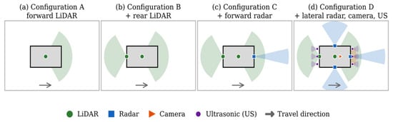
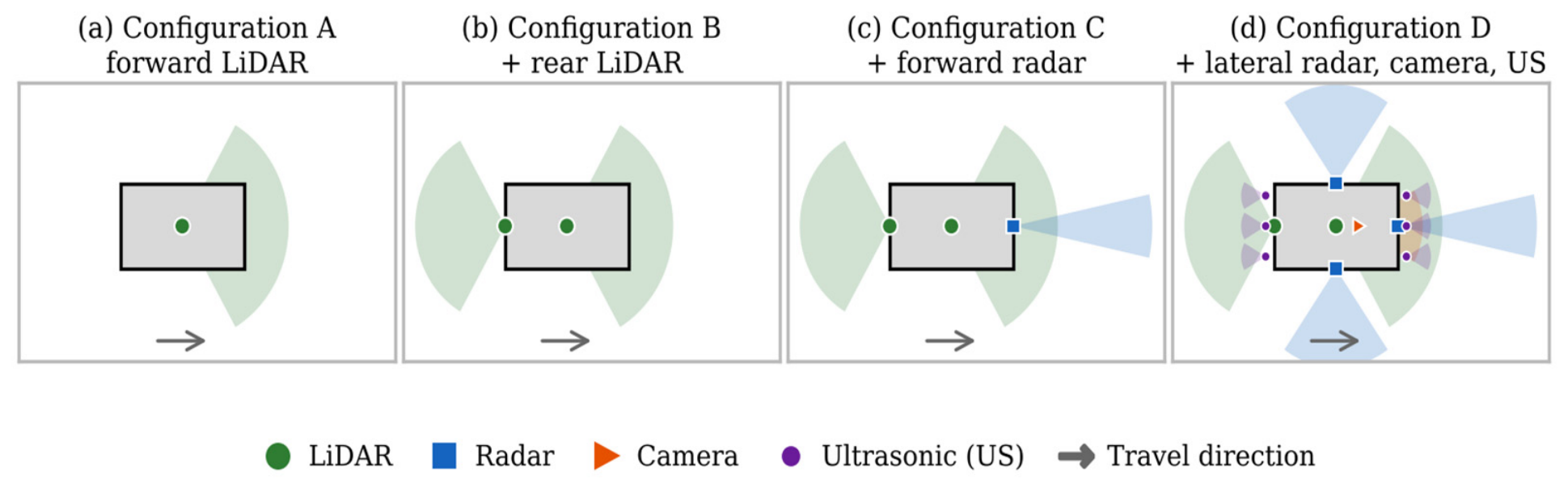
The primary (forward) LiDAR and, in Configuration D, the forward camera are mounted on a roof-center position for the broadest unobstructed forward view. The rear LiDAR (Configurations B–D) is mounted lower and tilted downward to cover the rear arc and improve near-field detection behind the truck. The forward radar (Configurations C–D) is mounted on the front bumper for long-range detection in poor visibility, while Configuration D’s two side radars and six ultrasonic sensors located at the front and rear bumpers address lateral and close-range blind spots. We designed four sensor configurations progressively: A (forward LiDAR only), B (adds rear LiDAR), C (adds forward radar), and D (comprehensive multimodal system), as illustrated in Figure 1 and summarized in Table 1.
Figure 1.
Top-view schematic of Configurations A to D on Caterpillar 797F.
Table 1.
Sensor configurations and simulation parameters (x forward, y right, origin at the truck center, ground level; αs,ideal = 1; L/H/S = light/heavy/severe).
3.3. Coverage Analysis Methodology
Coverage was assessed through geometric line-of-sight (LOS) visibility on a layered polar grid (r = 0.5 − 50 m, Δr = 0.5 m; θ = 0°−359.5°, Δθ = 0.5°; z ∈ {0.25, 1.8, 4.5} m), resulting in 72,000 points per layer. Grid cells overlapping the truck footprint are omitted from the valid region Ω. For sensor s under condition e, the effective range is adjusted using a degradation factor derived from the literature.
where Rnom,s is the nominal range and αs,e ∈ [0,1] is dimensionless (αs,ideal = 1). This is a simplified sensitivity-scaling model, not a fundamental propagation law; it is used only to test coverage sensitivity to degraded range, consistent with [4,5]. The light, heavy, and severe levels are comparative scenarios, not measured dust concentrations. Values of αs,e (Table 1) follow reported modality robustness: optical sensors (LiDAR, camera) are reduced most because dust and lens contamination degrade their returns [4,5,9], and radar is reduced least because it tolerates dust and rain [7,8].
Point inclusion in sensor s’s field of view follows standard vehicle-mounted sensor-coverage geometry [10,11]. For sensor s at position qs, ds(p) is the Euclidean distance to point p, and φs(p) and ψs(p) are the azimuth and elevation offsets from its boresight. Fs(p) = 1 when |φs| ≤ Hs/2 and |ψs| ≤ Vs/2, where Hs and Vs are the horizontal and vertical FOV.
The LOS indicator Ls(p) = 1 when the segment from qs to p is not intersected by the simplified truck-body occlusion geometry, and 0 otherwise. A point is covered by sensor s only when FOV, range, and LOS are simultaneously satisfied, where is the indicator function:
Overall multi-sensor coverage is the union of active sensor masks:
Coverage is reported as the area-weighted percentage , where Ap = rpΔrΔθ is the true annular-sector area of point p, to account for the non-uniform physical area of the polar sampling grid. Overall coverage is the mean of the three height layers.
3.4. Blind-Spot Identification
Blind points are points with Ce(p) = 0 in Equation (3). The overall blind area, weighted by area, is categorized into zones based on proximity: immediate (0–1 m), near-field (1–10 m), and far-field (>10 m). These zones are used for comparison purposes and are not linked to regulatory risk thresholds.
3.5. Redundancy Calculation
Geometric redundancy refers to the number of sensors that independently meet Equation (2) at a point. This acts as an overlap metric, not a certified functional-safety redundancy. Overlap is defined as the percentage of the covered area visible to two or more sensors. Sensitivity to removing one sensor measures how much the covered area decreases when that sensor is absent, expressed as its unique percentage-point contribution to overall coverage.
4. Results
4.1. Overall and Per-Layer Coverage
Table 2 reports overall area-weighted coverage for each configuration and condition, using the annular-sector weighting of Section 3.3.
Table 2.
Area-Weighted Coverage by Configuration and Condition.
Coverage increases steadily with the complexity of the configuration (A < B < C < D). For configurations A through C, coverage remains the same across ideal, light, and heavy conditions, decreasing only at the severe level because forward LiDAR and radar, with their typical ranges of 100 m and 150 m, respectively, exceed the 50 m grid unless severe range scaling is applied. In contrast, Configuration D includes lateral radars with a 50 m nominal range, whose effective range falls inside the grid as conditions worsen, resulting in a more gradual degradation of coverage.
For A–C, the elevated layer (4.5 m) is highest and the ground layer (0.25 m) is lowest, as mounting favors upward/outward FOV. However, D reverses this pattern (93.3% ground, 96.0% mid, 86.9% elevated) because its lower-mounted, narrow-vertical-FOV sensors significantly enhance ground and mid coverage.
4.2. Blind-Spot Distribution
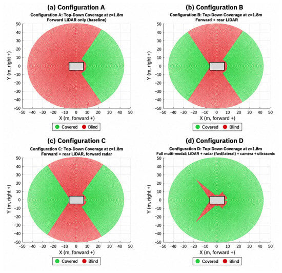
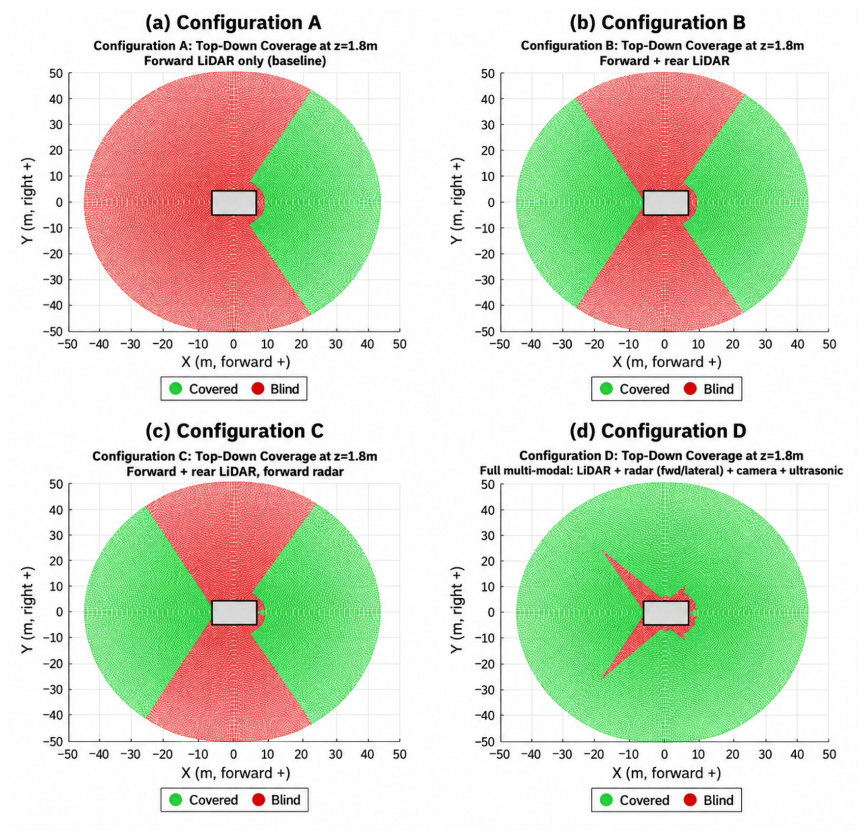
Figure 2 illustrates top-down coverage at mid-height (1.8 m) under ideal conditions. Configuration A (a) provides coverage only in a forward cone, with the rear 240° blind spot. B (b) covers the rear arc but has two lateral gaps. C (c) appears nearly identical to B because the forward radar’s beam overlaps with the LiDAR’s cone. D (d) closes both lateral gaps. Two narrow blind wedges remain at the rear lateral seams, extending roughly 28 m from the rear corners, with small notches at the vehicle body.
Figure 2.
Top-down geometric coverage at ideal conditions, mid-height layer (z = 1.8 m): (a) Configuration A; (b) Configuration B; (c) Configuration C; (d) Configuration D. Green = covered; red = blind. The gray rectangle is the truck footprint (top-down view).
Far-field blind area falls an order of magnitude from A to D (14,183 m2 to 921 m2); immediate-zone area barely changes (118 to 111 m2), since added sensors mainly extend coverage outward rather than closing near-vehicle gaps.
4.3. Redundancy and Single-Sensor Removal Sensitivity
Configuration A clearly shows 0% overlap with one sensor. B also exhibits 0% overlap: forward and rear LiDAR cones, each with a 120° FOV and facing opposite directions, create two 60° gaps instead of overlapping, so dual LiDAR provides additional coverage without redundancy for failure. C demonstrates moderate overlap, averaging around 7.95% in ideal conditions and 5.78% under severe conditions, mainly because the forward radar largely duplicates the LiDAR cone. D shows a 31.9% overlap under ideal circumstances, which reduces to 7.2% in severe conditions as different sensor pairs degrade at different rates.
Two key findings emerge: the forward radar’s contribution in C increases by a factor of about 85 from ideal to severe conditions (0.06% to 5.1%). Additionally, the rear LiDAR offers the greatest unique coverage among all tested sensors, making it the most critical single point of failure. Meanwhile, the camera’s contribution remains at 0.0% throughout, indicating it serves as a supplementary aid rather than a primary coverage source.
5. Discussion and Design Implications
Results translate into four implications for configuration selection, positioning, and mitigation (thresholds are study-defined):
(1) A is unsuitable for reversing or personnel proximity within its 240° rear blind arc. (2) B or C suit routes avoiding the two lateral gaps; dual LiDAR adds no failure redundancy. (3) Radar’s benefit concentrates in degraded conditions. (4) D suits any-direction approach, with the largest advantage in heavy/severe conditions, though small near-field notches and reduced severe-condition redundancy (31.9% to 7.2%) remain.
D’s lateral radars each carry more coverage loss (18.0%) than the forward radar, camera, or ultrasonic units. By zone: immediate (0–1 m) barely improves and is never eliminated; near-field (1–10 m) improves modestly; far-field (>10 m) benefits most, supporting D for extended-range hazard detection.
5.1. Sensitivity to Placement and Calibration Error
These errors were not simulated directly, but their first-order effects follow from the coverage geometry. A yaw error δ rotates a field of view by δ. Where adjacent fields of view do not overlap (Configuration B), the covered area is unchanged, and the gaps shift by δ. Where two fields of view overlap by less than δ, a blind wedge opens at their seam; the rear lateral wedges widen or narrow directly with the yaw of the adjacent sensors. A position offset shifts coverage boundaries by the same distance, mainly in the immediate and near-field zones. Range errors matter only when Reff,s,e falls below the 50 m grid radius (Table 2). Future work will investigate these effects through Monte Carlo simulations that introduce variations in sensor mounting position, yaw, and pitch to quantify coverage sensitivity and robustness.
5.2. Path to Experimental Validation
Each simulated role maps to commercial hardware: the Ouster OS2 LiDAR (Ouster, Inc., San Francisco, CA, USA; 200 m at 10% reflectivity, 360° × 22.5° FOV, IP68/IP69K) [15]; the ARS540 4D imaging radar (AUMOVIO SE, Frankfurt am Main, Germany; 300 m, ±60° FOV) for the forward role [16]; the smartmicro UMRR-96 Type 153 radar (s.m.s, smart microwave sensors GmbH, Braunschweig, Germany; up to 120 m, 100° to 130° horizontal FOV, IP67) for the lateral role [17]; and the Brigade Backscan BS-4000W ultrasonic system (Brigade Electronics Group plc, South Darenth, UK; 2.5 m, IP68 sensors) [18]. Their tolerance of haul truck shock, vibration, and dust must be confirmed with suppliers. Validation can proceed from static coverage mapping around a stationary truck, to controlled dust tests that measure αs,e, to field trials on active haul routes.
6. Conclusions
This study utilized a geometric line-of-sight approach to assess four sensor setups for 360° perception across four conditions. Ideally, coverage increased from 32.5% to 92.1% and, under severe conditions, from 19.8% to 68.9%. Redundancy and coverage were distinct; adding a second LiDAR increased coverage without overlap, while D’s overlap decreased from 31.9% to 7.2% as sensors degraded unevenly. The rear LiDAR was the most valuable sensor position, and the forward radar’s contribution grew by a factor of about 85 under degradation. These results only describe simulated geometric visibility and must not be considered as replacement for certified functional safety. Furthermore, the results are purely based on simulated studies and no field measurements were made. The model simplifies vehicle geometry for occlusion, uses literature-based scaling for degradation, and uses generic sensor specifications, so coverage values are best read as comparisons between configurations. Experimental validation following Section 5 is the next step.
Author Contributions
N.Y.D.A.; original draft preparation and editing, S.F. and M.A.R.; review and supervision. All authors have read and agreed to the published version of the manuscript.
Funding
This research was funded by the Centers for Disease Control and Prevention and the National Institute for Occupational Safety and Health (CDC-NIOSH-U60OH012685-01-00), Research and Technological Innovations in Automation, Robotics, and Intelligent Mining Systems for Transformative Improvements in Workplace Safety, Health, and Efficiencies.
Institutional Review Board Statement
Not applicable.
Informed Consent Statement
Not applicable.
Data Availability Statement
The simulation data supporting the findings are available from the corresponding author on reasonable request.
Conflicts of Interest
The authors declare no conflict of interest.
Abbreviations
The following abbreviations are used in this manuscript:
| AHSs | Autonomous Haulage Systems |
| LiDAR | Light Detection and Ranging |
| mmWave | Millimeter-wave |
| FOV | Field of View |
References
- Chen, L.; Li, Y.; Li, L.; Qi, S.; Zhou, J.; Tang, Y.; Yang, J.; Xin, J. High-Precision Positioning, Perception and Safe Navigation for Automated Heavy-Duty Mining Trucks. IEEE Trans. Intell. Veh. 2024, 9, 4644–4656. [Google Scholar] [CrossRef] [Scilit]
- Afzalaghaeinaeini, A.; Seo, J.; Lee, D.; Lee, H. Design of Dust-Filtering Algorithms for LiDAR Sensors Using Intensity and Range Information in Off-Road Vehicles. Sensors 2022, 22, 4051. [Google Scholar] [CrossRef] [Scilit] [PubMed]
- Jiang, X.; Xie, Y.; Na, C.; Yu, W.; Meng, Y. Algorithm for Point Cloud Dust Filtering of LiDAR for Autonomous Vehicles in Mining Area. Sustainability 2024, 16, 2827. [Google Scholar] [CrossRef] [Scilit]
- Phillips, T.G.; Guenther, N.; McAree, P.R. When the Dust Settles: The Four Behaviors of LiDAR in the Presence of Fine Airborne Particulates. J. Field Robot. 2017, 34, 985–1009. [Google Scholar] [CrossRef] [Scilit]
- Alavi, B.; Illing, T.; Campean, F.; Spencer, P.; Abdullatif, A. Quantifying Automotive Lidar System Uncertainty in Adverse Weather: Mathematical Models and Validation. Appl. Sci. 2025, 15, 8191. [Google Scholar] [CrossRef] [Scilit]
- Schlager, B.; Goelles, T.; Muckenhuber, S.; Watzenig, D. Contaminations on Lidar Sensor Covers: Performance Degradation Including Fault Detection and Modeling as Potential Applications. IEEE Open J. Intell. Transp. Syst. 2022, 3, 738–747. [Google Scholar] [CrossRef] [Scilit]
- Peng, X.; Tang, M.; Sun, H.; Bierzynski, K.; Servadei, L.; Wille, R. 4D mmWave Radar for Sensing Enhancement in Adverse Environments: Advances and Challenges. In Proceedings of the 2025 IEEE 28th International Conference on Intelligent Transportation Systems (ITSC); IEEE: Piscataway, NJ, USA, 2025; pp. 2884–2891. [Google Scholar]
- Zang, S.; Ding, M.; Smith, D.; Tyler, P.; Rakotoarivelo, T.; Kaafar, M.A. The Impact of Adverse Weather Conditions on Autonomous Vehicles: How Rain, Snow, Fog, and Hail Affect the Performance of a Self-Driving Car. IEEE Veh. Technol. Mag. 2019, 14, 103–111. [Google Scholar] [CrossRef] [Scilit]
- Vargas, J.; Alsweiss, S.; Toker, O.; Razdan, R.; Santos, J. An Overview of Autonomous Vehicles Sensors and Their Vulnerability to Weather Conditions. Sensors 2021, 21, 5397. [Google Scholar] [CrossRef] [Scilit] [PubMed]
- Hafemann, P.; Hahn, S.E.; Lienkamp, M. Optimizing Autonomous Vehicle Sensor Setups: A Framework for Coverage Analysis. In Proceedings of the 2023 IEEE Symposium Sensor Data Fusion and International Conference on Multisensor Fusion and Integration (SDF-MFI); IEEE: Piscataway, NJ, USA, 2023. [Google Scholar]
- Hartstern, M.; Rack, V.; Stork, W. Conceptual Design of Automotive Sensor Systems: Analyzing the Impact of Different Sensor Positions on Surround-View Coverage. In Proceedings of the 2020 IEEE SENSORS, Rotterdam, The Netherlands, 25–28 October 2020; pp. 1–4. [Google Scholar] [CrossRef] [Scilit]
- Yeong, D.J.; Velasco-Hernandez, G.; Barry, J.; Walsh, J. Sensor and Sensor Fusion Technology in Autonomous Vehicles: A Review. Sensors 2021, 21, 2140. [Google Scholar] [CrossRef] [Scilit] [PubMed]
- Wang, Z.; Wu, Y.; Niu, Q. Multi-Sensor Fusion in Automated Driving: A Survey. IEEE Access 2020, 8, 2847–2868. [Google Scholar] [CrossRef] [Scilit]
- Caterpillar Inc. Cat 797F Mining Truck: Technical Specifications; Publication No. AEHQ5884-09; Caterpillar Inc.: Peoria, IL, USA, 2023; Available online: https://caterpillar.scene7.com/is/content/Caterpillar/CM20221101-213a6-5a873 (accessed on 14 August 2026).
- Ouster Inc. OS2 Long-Range Digital Lidar Sensor, Rev 7 Datasheet. Available online: https://autonomoustuff.com/products/ouster-os2 (accessed on 18 October 2026).
- AUMOVIO (Formerly Continental Automotive). ARS540 Advanced Radar Sensor. Available online: https://www.aumovio.com/en/solutions/driver-assistance/automated-assisted-driving/radar-technology/ars540.html (accessed on 18 October 2026).
- Smartmicro. Automotive Radar UMRR-96 Type 153. Available online: https://autonomoustuff.com/products/smartmicro-automotive-radar-umrr-96 (accessed on 18 October 2026).
- Brigade Electronics. Backscan BS-4000W Ultrasonic Detection System. Available online: https://brigade-electronics.com/detection-systems/ultrasonic-sensors/backscan/ (accessed on 18 October 2026).

Disclaimer/Publisher’s Note: The statements, opinions and data contained in all publications are solely those of the individual author(s) and contributor(s) and not of MDPI and/or the editor(s). MDPI and/or the editor(s) disclaim responsibility for any injury to people or property resulting from any ideas, methods, instructions or products referred to in the content. |
© 2026 by the authors. Licensee MDPI, Basel, Switzerland. This article is an open access article distributed under the terms and conditions of the Creative Commons Attribution (CC BY) license.