


Abstract
Low-cost IoT soil sensors are attractive for precision agriculture because they can record field conditions continuously and at low cost. However, when machine learning models are trained on dense time-series data, their reported accuracy can be misleading if their temporal structure is ignored. This study examined Random Forest prediction of sensor-derived nitrogen (N), phosphorus (P), and potassium (K) readings using 63,769 observations collected over 170 days from two LoRa-based soil-sensing nodes in a tropical field site in Thailand. Soil moisture, temperature, electrical conductivity (EC), and pH were used as inputs; the outputs were the N, P, and K values reported by the composite sensor, not laboratory-confirmed nutrient concentrations. Model evaluation compared repeated random split (RS) validation with chronological split (CS) validation. RS gave high apparent performance (–0.901), but CS failed for all targets (, , and for N, P, and K, respectively). Jensen–Shannon divergence values of 0.070–0.256 indicated measurable train–test distributional drift. SHAP analysis further showed that EC and temperature were the main contributors on average, while humidity contributed least in most validation–target combinations. The findings suggest that random-split validation can greatly overstate the usefulness of ML models for future IoT soil-sensor data. Time-aware validation, periodic laboratory calibration, and cautious interpretation are therefore essential before sensor-derived NPK predictions are used for agronomic decisions.
1. Introduction
Low-cost Internet of Things (IoT) soil sensors can provide continuous field-scale information for precision agriculture, but the reliability of machine learning (ML) models trained on such data remains uncertain [1]. Laboratory analysis remains the standard method for quantifying soil nitrogen (N), phosphorus (P), and potassium (K), yet it is costly and temporally sparse. Composite low-cost sensors offer a practical alternative for monitoring, but reported NPK values should be interpreted as sensor-derived readings unless calibrated against laboratory reference measurements [2,3,4].
Low-cost composite NPK probes are particularly sensitive to this problem because the reported N, P, and K values are generated from a shared soil–electrode response [4]. Consequently, high apparent predictive accuracy may reflect stable electrical or thermal sensor behavior rather than nutrient-specific chemistry. This distinction is central for smart-agriculture deployment: an algorithm can reproduce the readings reported by a sensor without necessarily estimating laboratory-confirmed soil fertility.
A major methodological risk in IoT time-series modeling is temporal data leakage. Sensor readings recorded every few minutes are highly autocorrelated; when these observations are randomly shuffled, test samples are surrounded by near-duplicate training samples. Such random split (RS) validation can therefore measure interpolation among adjacent records rather than future predictive ability [5,6,7,8]. This issue is especially important under tropical field conditions, where soil moisture, EC, temperature, and sensor response can drift across wet–dry periods [9].
This study evaluates whether a Random Forest model can generalize to future sensor-derived NPK readings from a 170-day tropical IoT soil-monitoring dataset. The specific objectives were to (i) compare RS and chronological split (CS) validation, (ii) quantify train–test distributional drift, and (iii) use SHAP to identify which sensor variables drive model predictions.
2. Materials and Methods
2.1. Field Deployment and Dataset
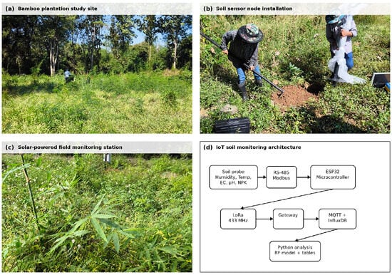
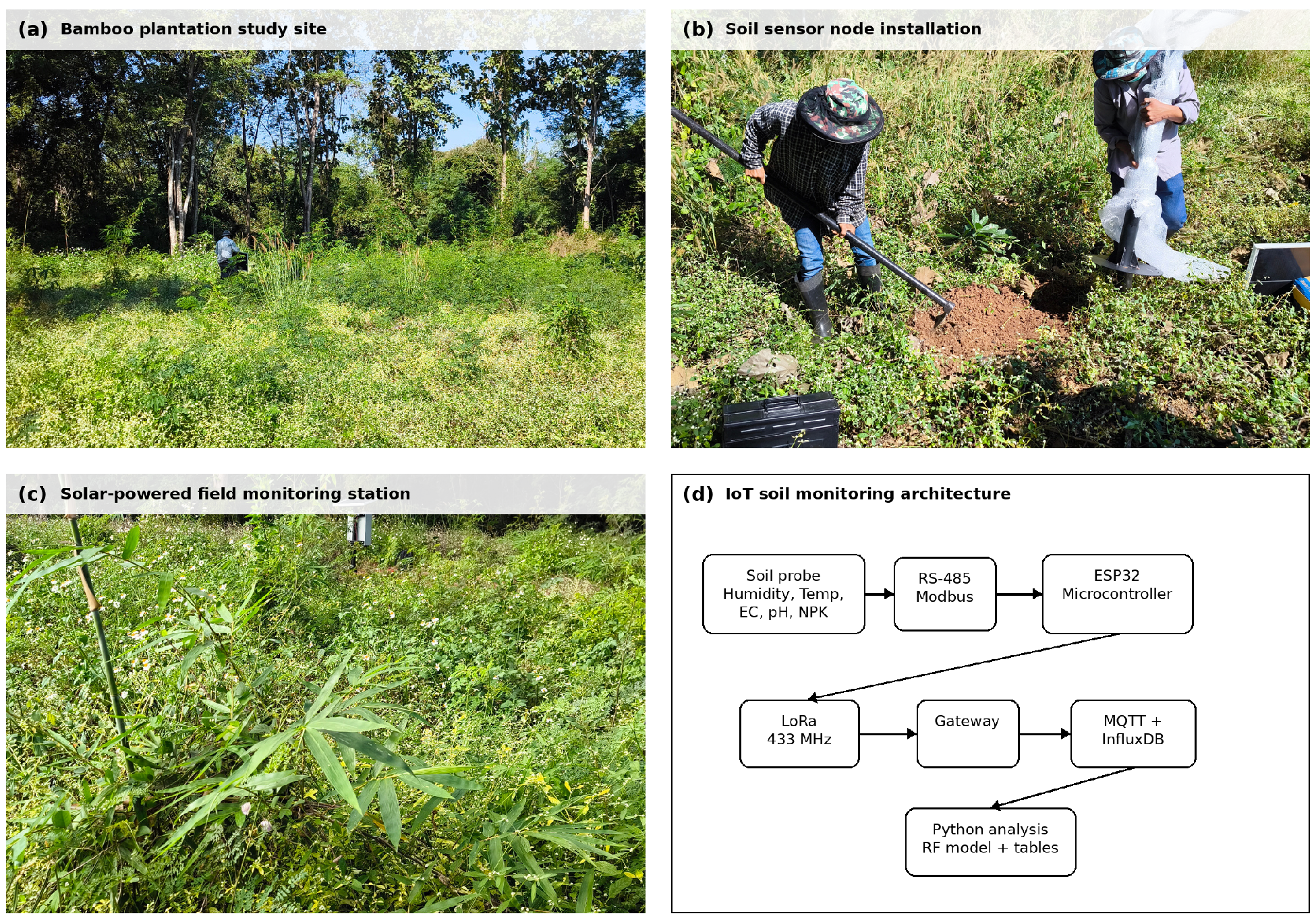
Two LoRa-based soil-sensing nodes were installed at a tropical agricultural field site in Thailand. Each node used an RS-485 Modbus composite soil probe to record moisture, temperature, EC, pH, and sensor-reported NPK values. Readings were transmitted by LoRa and stored in a cloud time-series database. Data were logged every 5 min for 170 days, producing 63,769 raw observations. The field deployment and data-acquisition architecture are shown in Figure 1. No concurrent laboratory measurements were collected; therefore, the N, P, and K variables analyzed here are sensor-derived readings and not independently validated soil fertility measurements.
Figure 1.
Field deployment and IoT architecture: (a) bamboo plantation study site, (b) sensor-node installation, (c) solar-powered monitoring station, and (d) sensing and data pipeline.
Records with missing values, communication-error codes, or values outside the rated sensor range were removed. Remaining outliers were filtered using a 3 rule applied independently for each channel and node. After cleaning, 59,236 observations remained (92.9% of the raw total). Lag-1 autocorrelation for the NPK channels exceeded 0.97, confirming that adjacent 5 min records were near-duplicates.
2.2. Modeling, Validation, and Interpretation
A multi-output Random Forest regressor [10] was trained using four inputs: moisture, temperature, EC, and pH. The three outputs were sensor-derived N, P, and K readings. The selected model used 200 trees, maximum depth 20, minimum leaf size 4, and bootstrapped sampling. A simple multi-output linear regression baseline was also evaluated to test whether the observed validation gap was model-specific.
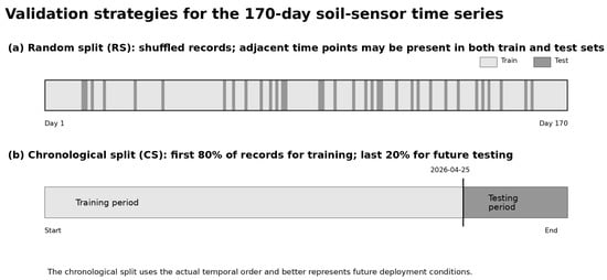
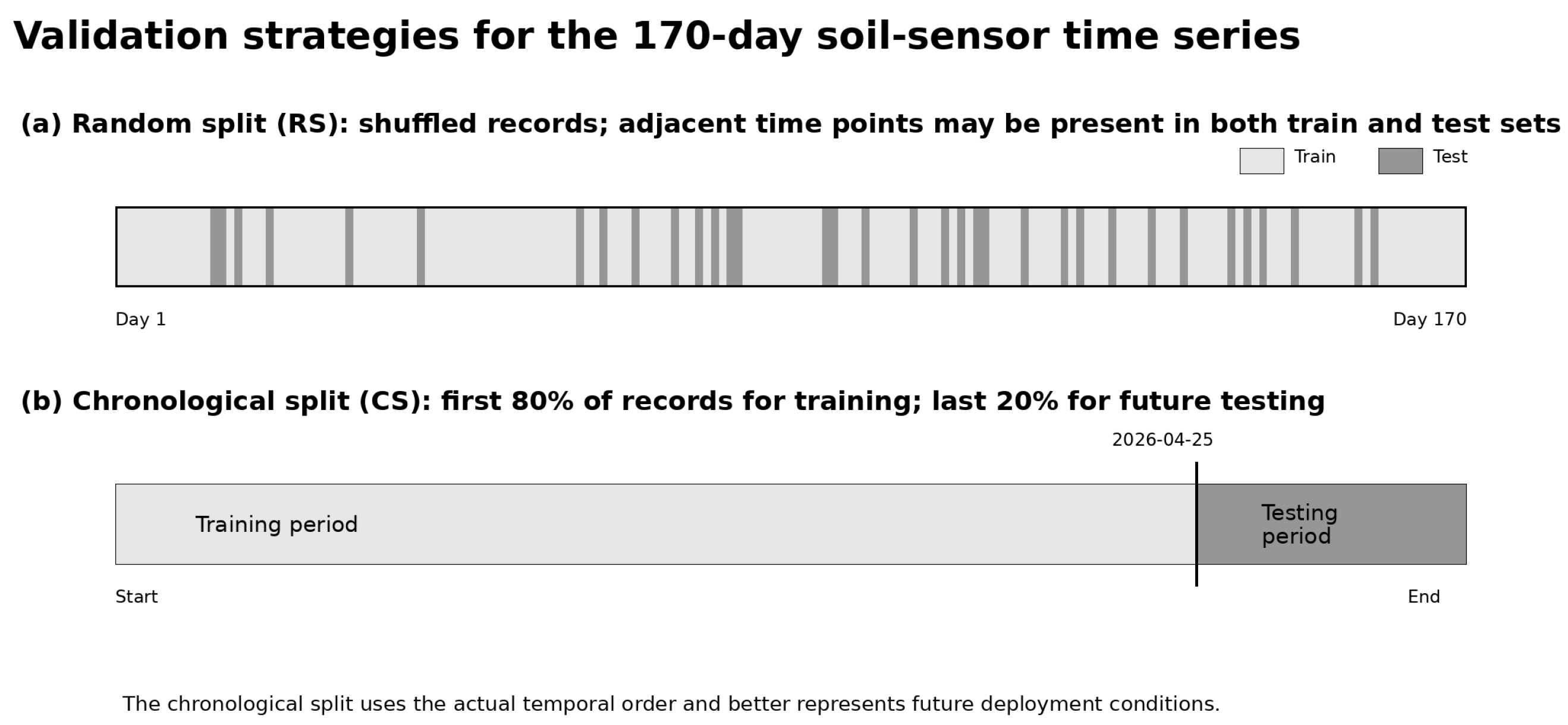
Two validation strategies were compared. In RS, the cleaned observations were randomly split into 80% training and 20% testing data; the RS experiment was repeated using five seeds and reported as mean ± SD. In CS, the first 80% of the time-ordered record formed the training set and the final 20% formed the test set. Performance was measured using , RMSE, and MAE. Train–test distributional drift was summarized using Jensen–Shannon divergence (JSD) [11]. TreeSHAP was computed separately for each output by fitting independent single-output Random Forest models for N, P, and K under the same validation settings [12,13]. The two validation strategies are illustrated in Figure 2.
Figure 2.
Comparison of validation strategies. Random split shuffles autocorrelated records, whereas chronological split trains on earlier observations and tests on future observations.
2.3. Use of Generative AI
Generative AI was used in a supporting role in this study. The large language model Claude (Anthropic) was used to assist with writing and debugging the Python 3.14 scripts for data cleaning, model fitting, and figure generation, and to improve the clarity of the English text. The authors executed all code on their own data, checked every reported value against the script output, and reviewed and edited all AI-assisted text. No AI tool generated or altered the experimental data, and no AI tool is listed as an author.
3. Results and Discussion
3.1. Temporal Patterns and Validation Design
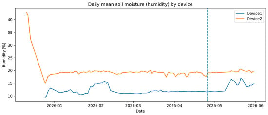
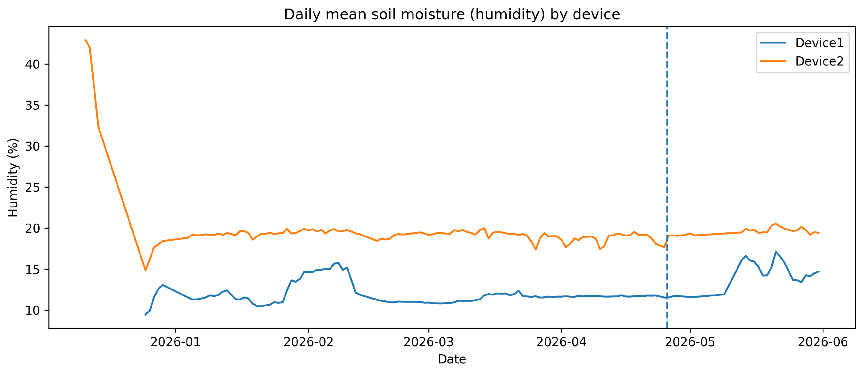
The daily soil-moisture pattern in Figure 3 illustrates the non-stationary nature of the field dataset and the need for time-aware validation. Device 1 and Device 2 showed different absolute moisture levels, indicating local node-to-node variability. Nevertheless, both nodes were affected by temporal structure and therefore cannot be treated as independent, randomly exchangeable observations.
Figure 3.
Daily mean soil moisture (reported by the sensor as humidity) for the two monitoring nodes. The dashed line indicates the boundary between the chronological training and testing periods.
3.2. Random Split Strongly Overestimated Future Performance
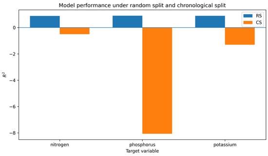
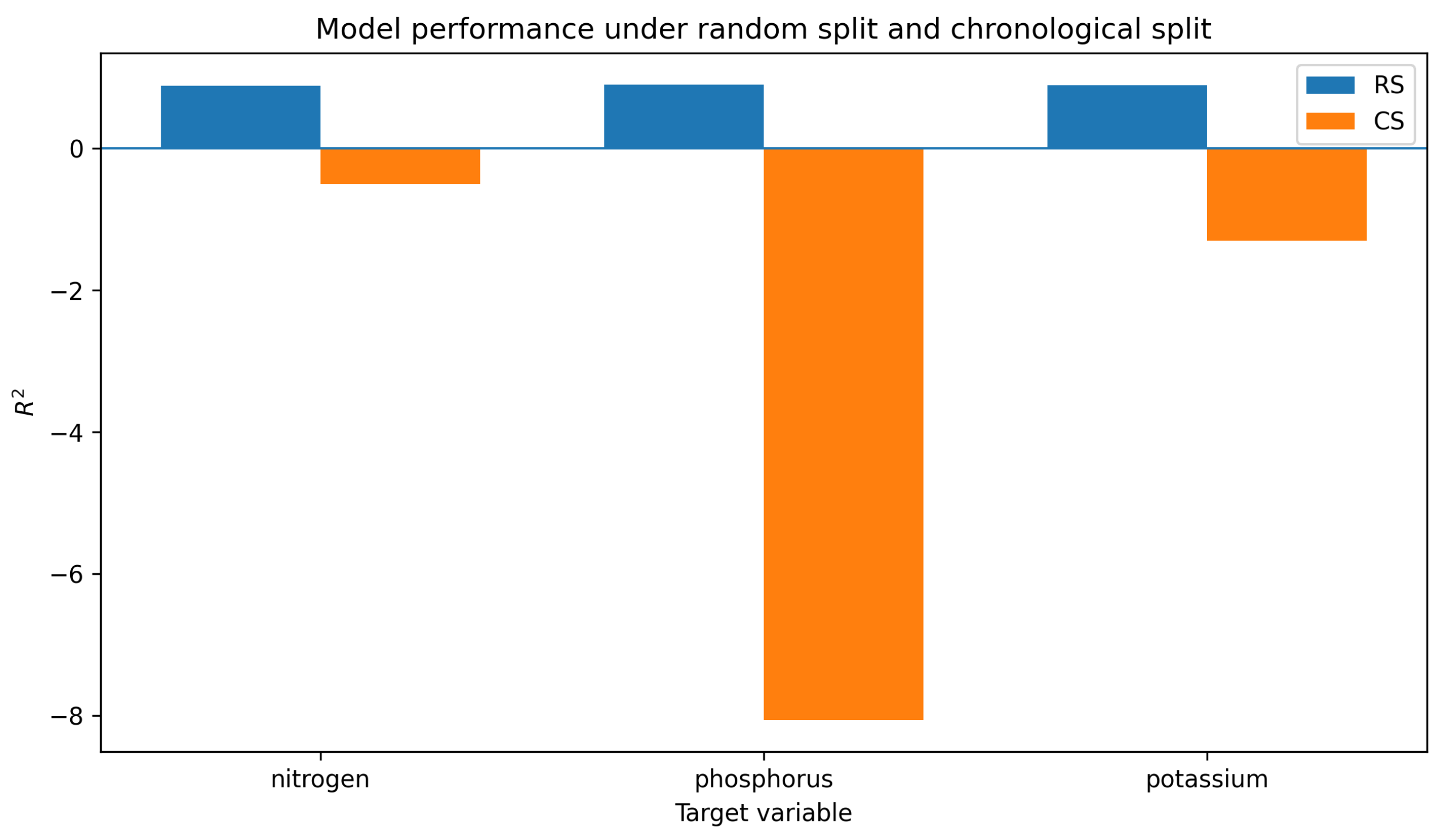
RS validation produced high apparent accuracy for all targets ( = 0.890–0.901), but CS validation produced negative for N, P, and K (Table 1). The largest failure occurred for phosphorus ( = −8.062), indicating a complete loss of generalization to future observations. The low between-seed variation in RS results shows that the high RS performance was not caused by a particular random seed; rather, it was a stable consequence of temporal leakage. Because lag-1 autocorrelation exceeded 0.97, random splitting allowed the model to interpolate between near-duplicate 5 min observations instead of predicting genuine future sensor behavior. The RS–CS performance comparison is presented in Figure 4.
Table 1.
Random Forest performance under repeated random split (RS; five seeds, mean ± SD) and chronological split (CS) validation.
Figure 4.
Random Forest model performance under random split and chronological split validation. The negative chronological-split values indicate poor generalization to future observations.
JSD values of 0.070–0.256 confirmed measurable distributional drift between the chronological training and testing periods. Mean humidity increased from 15.12 ± 3.98% to 16.81 ± 3.16%, EC increased from 103.61 ± 89.82 to 154.37 ± 82.91, and temperature increased from 27.89 ± 3.35 to 30.28 ± 1.38 °C. These shifts explain why relationships learned during the training period transferred poorly to the future test period.
3.3. Sensor-Response Structure Drove the Model
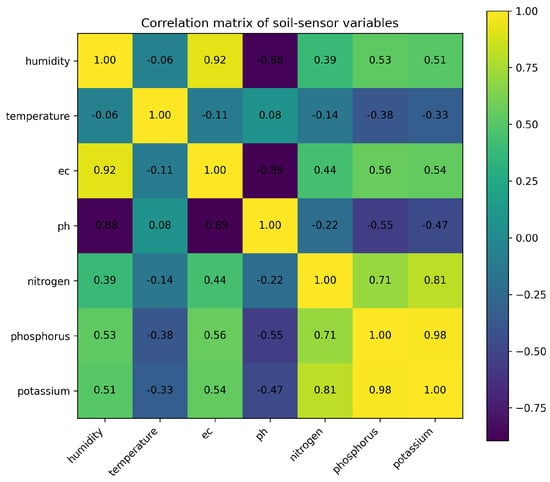
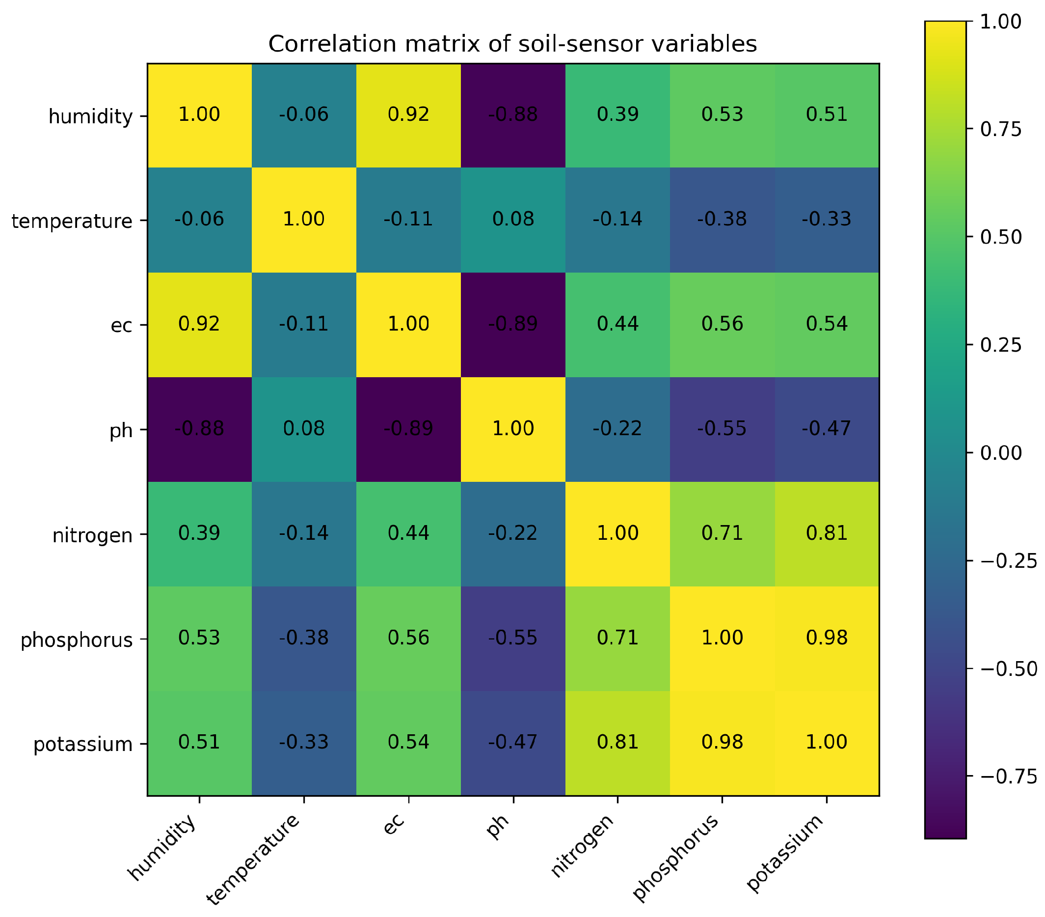
The SHAP results showed that EC was the largest contributor on average (approximately 46.8%), while temperature was also highly influential (approximately 37.9%). Temperature exceeded EC in the CS nitrogen case, although its bivariate correlations with the NPK channels were weak or negative. This apparent disagreement between correlation and SHAP is expected: correlation measures pairwise linear association, whereas SHAP measures marginal contribution inside a nonlinear model after accounting for the other predictors. Temperature therefore likely acted as a contextual variable for time-dependent sensor-response regimes rather than as a nutrient-specific chemical driver. The correlations among sensor variables are shown in Figure 5.
Figure 5.
Correlation matrix of the main soil-sensor variables. The associations among humidity, EC, and sensor-derived NPK readings indicate shared sensor and electrical-response structure.
The feature contributions for each nutrient target and validation strategy are summarized in Table 2. The difference between correlation and SHAP is also instructive. Correlation is a pairwise linear summary, whereas SHAP estimates the contribution of a variable inside the trained nonlinear model conditional on the other predictors. Thus, temperature can show weak or negative simple correlations with NPK readings while still helping the RF model separate time-dependent regimes. This behavior is consistent with a system in which temperature modifies electrode response, ionic mobility [14], or the sensor firmware’s mapping from electrical response to nominal NPK values.
Table 2.
Relative mean absolute SHAP importance (%) computed separately for each sensor-derived NPK target and validation strategy.
The correlation matrix and SHAP analysis together suggest that the model learned sensor-response behavior rather than independent soil chemistry. Low-cost composite NPK probes are influenced by ionic conductance, moisture condition, electrode–soil contact, and temperature. Without laboratory calibration, their NPK outputs should therefore be treated as sensor-derived indicators. The practical implication is that an apparently accurate RS model can be unsuitable for future agronomic decision-making if it has only learned temporally local sensor-response patterns.
A linear-regression baseline showed lower performance but the same general validation sensitivity: RS mean ranged from 0.373 to 0.429, whereas CS ranged from −22.047 to 0.042. Node-level chronological analysis also showed performance differences between the two devices, indicating that local soil heterogeneity and node-to-node variation should be considered in future multi-node deployments.
4. Limitations and Practical Implications
This study should be interpreted as a reliability assessment of sensor-derived NPK prediction rather than a laboratory-validated soil-fertility study. The absence of concurrent Kjeldahl N, Bray–Kurtz P, or exchangeable K measurements prevents direct claims about true nutrient concentrations. The most defensible interpretation is therefore that the models predicted the numerical outputs reported by low-cost composite sensors, while the chronological validation test revealed how poorly those learned relationships generalized to future sensor-response regimes.
The deployment also used only two sensor nodes. This design was sufficient to expose temporal leakage and distributional drift, but it cannot fully separate sensor-to-sensor variation from microsite soil heterogeneity. Future work should include more nodes, repeated installation depths, periodic laboratory reference samples, and longer multi-season monitoring. Such data would allow for a stronger distinction between real nutrient dynamics, local soil variability, sensor drift, and communication-related artifacts.
For practitioners, the main recommendation is to treat random-split performance as an optimistic upper bound rather than an estimate of field performance. Models intended for deployment should be evaluated with chronological, blocked, or rolling-origin validation. They should also be accompanied by drift monitoring and periodic laboratory calibration before their outputs are used for fertilizer recommendations.
In a bamboo plantation or other perennial field system, the practical value of an IoT sensor network is not limited to direct nutrient estimation. Continuous measurements can still help identify periods of unusually dry soil, abrupt EC changes after rainfall or fertigation, node-specific drift, and possible sensor contact problems. These signals are useful for field supervision, but they should be treated differently from laboratory-confirmed fertility data. A conservative workflow is therefore to use the low-cost sensors for continuous situational awareness and to reserve fertilizer recommendations for cases where sensor patterns have been anchored to periodic soil sampling. This interpretation also helps explain the apparently contradictory result observed in this study: the model could learn the numerical behavior of the sensor under RS, but that behavior did not remain stable when future observations were used for testing.
A practical calibration plan for future work would be relatively simple. First, soil samples should be collected around each node at the same depth as the probe and analyzed for pH, EC, organic matter, available P, exchangeable K, and an appropriate N indicator. Second, sampling should be repeated across contrasting field conditions rather than conducted only once; for example, after rainfall, during a dry period, and after fertilizer application. Third, calibration should be evaluated with a chronological split so that the laboratory-anchored model is tested on later samples rather than on randomly shuffled observations. Finally, calibration results should be reported separately for each node before being pooled. This would make it possible to distinguish a general sensor response from local soil heterogeneity or a poorly seated probe. Such a protocol would not remove the need for caution, but it would move low-cost IoT sensing closer to an agronomically interpretable decision-support tool.
5. Conclusions
Random-split validation substantially overestimated the predictive utility of ML models trained on continuous IoT soil-sensor data. Although RS produced high apparent performance ( = 0.890–0.901), chronological validation yielded negative values for all three sensor-derived NPK targets. This failure was explained by temporal leakage, high autocorrelation among adjacent records, and measurable distributional drift between the training and test periods. SHAP analysis further showed that predictions were driven mainly by EC, temperature, and sensor-context effects rather than laboratory-confirmed nutrient-specific chemistry.
For practical deployment, ML models for IoT soil sensing should be evaluated using chronological or blocked time-series validation, calibrated periodically against laboratory soil analyses, and monitored for distributional drift. Future work should combine longer multi-season datasets with laboratory reference measurements to separate true nutrient dynamics from sensor-response artifacts. In addition, reporting both RS and CS performance should become standard practice for IoT soil-sensor studies, because the gap between the two provides a direct diagnostic of temporal leakage and practical deployability.
Author Contributions
Conceptualization, K.P. and S.S.; methodology, K.P.; software, K.P.; validation, K.P. and D.W.; formal analysis, K.P.; investigation, K.P. and D.W.; data curation, K.P.; writing—original draft preparation, K.P.; writing—review and editing, S.S. and N.A.; visualization, K.P.; supervision, S.S. and N.A.; project administration, S.S. All authors have read and agreed to the published version of the manuscript.
Funding
This research received no external funding.
Institutional Review Board Statement
Not applicable.
Informed Consent Statement
Not applicable.
Data Availability Statement
The dataset will be made available upon reasonable request to the corresponding author.
Acknowledgments
During the preparation of this manuscript, the authors used Claude 4.7 (Anthropic) for the purposes described in Section 2.3, namely, assistance with analysis scripts and language editing. The authors have reviewed and edited the output and take full responsibility for the content of this publication.
Conflicts of Interest
The authors declare no conflicts of interest.
References
- Liakos, K.G.; Busato, P.; Moshou, D.; Pearson, S.; Bochtis, D. Machine learning in agriculture: A review. Sensors 2018, 18, 2674. [Google Scholar] [CrossRef] [Scilit]
- Adamchuk, V.I.; Hummel, J.W.; Morgan, M.T.; Upadhyaya, S.K. On-the-go soil sensors for precision agriculture. Comput. Electron. Agric. 2004, 44, 71–91. [Google Scholar] [CrossRef] [Scilit]
- Sinfield, J.V.; Fagerman, D.; Colic, O. Evaluation of sensing technologies for on-the-go soil nutrient detection. Comput. Electron. Agric. 2010, 70, 1–18. [Google Scholar] [CrossRef] [Scilit]
- Baldi, E.; Quartieri, M.; Chiarelli, G.; Tassinari, A.; Larocca, G.N.; Messini, M.; Toselli, M. Evaluation of the reliability of in situ, real-time probes for precise determination of nitrogen, phosphorus and potassium in agricultural crops. Horticulturae 2026, 12, 898. [Google Scholar] [CrossRef] [Scilit]
- Kapoor, S.; Narayanan, A. Leakage and the reproducibility crisis in machine-learning-based science. Patterns 2023, 4, 100804. [Google Scholar] [CrossRef] [Scilit]
- Roberts, D.R.; Bahn, V.; Ciuti, S.; Boyce, M.S.; Elith, J.; Guillera-Arroita, G.; Hauenstein, S.; Lahoz-Monfort, J.J.; Schröder, B.; Thuiller, W.; et al. Cross-validation strategies for data with temporal, spatial, hierarchical, or phylogenetic structure. Ecography 2017, 40, 913–929. [Google Scholar] [CrossRef] [Scilit]
- Bergmeir, C.; Benítez, J.M. On the use of cross-validation for time series predictor evaluation. Inf. Sci. 2012, 191, 192–213. [Google Scholar] [CrossRef] [Scilit]
- Cerqueira, V.; Torgo, L.; Mozetič, I. Evaluating time series forecasting models: An empirical study on performance estimation methods. Mach. Learn. 2020, 109, 1997–2028. [Google Scholar] [CrossRef] [Scilit]
- Webb, G.I.; Hyde, R.; Cao, H.; Nguyen, H.L.; Petitjean, F. Characterizing concept drift. Data Min. Knowl. Discov. 2016, 30, 964–994. [Google Scholar] [CrossRef] [Scilit]
- Breiman, L. Random forests. Mach. Learn. 2001, 45, 5–32. [Google Scholar] [CrossRef] [Scilit]
- Lin, J. Divergence measures based on the Shannon entropy. IEEE Trans. Inf. Theory 1991, 37, 145–151. [Google Scholar] [CrossRef] [Scilit]
- Lundberg, S.M.; Lee, S.-I. A unified approach to interpreting model predictions. Adv. Neural Inf. Process. Syst. 2017, 30, 4765–4774. [Google Scholar]
- Lundberg, S.M.; Erion, G.; Chen, H.; DeGrave, A.; Prutkin, J.M.; Nair, B.; Katz, R.; Himmelfarb, J.; Bansal, N.; Lee, S.-I. From local explanations to global understanding with explainable AI for trees. Nat. Mach. Intell. 2020, 2, 56–67. [Google Scholar] [CrossRef] [Scilit]
- Corwin, D.L.; Lesch, S.M. Apparent soil electrical conductivity measurements in agriculture. Comput. Electron. Agric. 2005, 46, 11–43. [Google Scholar] [CrossRef] [Scilit]

Disclaimer/Publisher’s Note: The statements, opinions and data contained in all publications are solely those of the individual author(s) and contributor(s) and not of MDPI and/or the editor(s). MDPI and/or the editor(s) disclaim responsibility for any injury to people or property resulting from any ideas, methods, instructions or products referred to in the content. |
© 2026 by the authors. Licensee MDPI, Basel, Switzerland. This article is an open access article distributed under the terms and conditions of the Creative Commons Attribution (CC BY) license.