


Abstract
Distributed generation (DG) interconnection in radial distribution networks is often evaluated through voltage-based hosting-capacity studies that lead to binary accept/reject decisions. This paper evaluates a two-stage optimal-power-flow (OPF)–machine-learning framework for rapid pre-feasibility screening. A revised AC optimal power flow (OPF) scenario set contains 20,000 cases spanning 21 candidate DG buses, active-power injections up to 1.8 MW, and loading factors from 0.45 to 1.10. Of 19,930 solver-successful cases, 12,300 satisfy the 0.95–1.05 p.u. engineering voltage criterion and 7630 are non-compliant. In Stage 1, a decision-tree classifier separates feasible and non-compliant cases using categorical DG location, P_DG, and loading factor α, achieving 97.41% accuracy, 97.91% F1-score, 96.37% specificity, and receiver operating characteristic area under the curve (ROC-AUC) = 0.9908 under stratified 10-fold cross-validation. In Stage 2, only feasible scenarios are passed to regression surrogates that predict the signed optimal reactive-power setpoint Q_DG*. The neural network achieves a coefficient of determination (R2) = 0.9996, root mean square error (RMSE) = 4.745 kVAr, and mean absolute error (MAE) = 1.964 kVAr. Surrogate inference requires microseconds per scenario compared with an average OPF solution time of 0.146 s. The framework is intended as a controlled pre-screening benchmark and does not replace detailed three-phase interconnection studies.
1. Introduction
The rapid growth of inverter-based distributed generation (DG), particularly photovoltaic generation, is reshaping radial distribution networks. Voltage-limit violations are among the main constraints identified in interconnection and hosting-capacity studies, which often lead to binary accept/reject decisions under a limited set of operating points [1,2,3,4]. Such decisions can be conservative because modern inverters can exchange reactive power and support voltage regulation, potentially enabling otherwise infeasible connections without immediate network reinforcement [5,6,7,8].
Optimization-based methods, including AC optimal power flow (AC–OPF), provide a rigorous way to quantify DG operation under network constraints [9,10]. Nevertheless, repeatedly solving nonlinear OPF problems for many candidate buses, DG sizes, and loading conditions may be computationally inconvenient for routine screening. The central hypothesis tested here is that the optimal signed DG reactive-power setpoint produced by AC–OPF can be approximated with engineering-useful accuracy from a reduced set of readily available interconnection variables—DG location, active-power injection, and feeder loading—so that repeated online OPF solutions can be avoided. AC–OPF is used as a physics-based reference rather than as an exact global benchmark: because the formulation is nonlinear and nonconvex, convergence and local-stationarity behavior can depend on initialization, active constraints, and network parameters. These limitations are considered explicitly in the revised scenario-generation procedure.
Building on previous work on reactive power support for DG integration [11], the framework contributes: (i) an explicit two-stage screening procedure in which a binary feasibility classifier first separates voltage-compliant and non-compliant operating points and a regression surrogate then estimates the signed reactive-power setpoint only for feasible cases; (ii) a reproducible AC–OPF scenario-generation process covering DG location, active-power level, and feeder loading; (iii) categorical encoding of DG location for ML training; and (iv) comparison of classification and regression models using out-of-fold performance, signed-residual statistics, and measured inference time. Standard supervised-learning formulations used for the surrogate models are described in [12,13,14].
The method is evaluated using a deliberately simplified single-phase representation of the IEEE 34-node test feeder [15,16]. Voltage regulators, shunt capacitors, and step-down transformers are removed to isolate the voltage–reactive-power relationship attributable to the candidate DG. This controlled benchmark is not intended to reproduce the full behavior of an actual unbalanced feeder; phase unbalance, device-control interactions, and detailed transformer effects are outside the present scope. Consequently, the engineering conclusions are restricted to proof-of-concept pre-feasibility screening, and extension to detailed three-phase networks is identified as future work.
2. Methodology
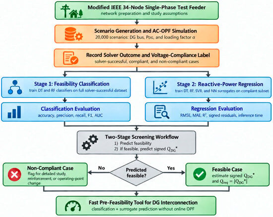
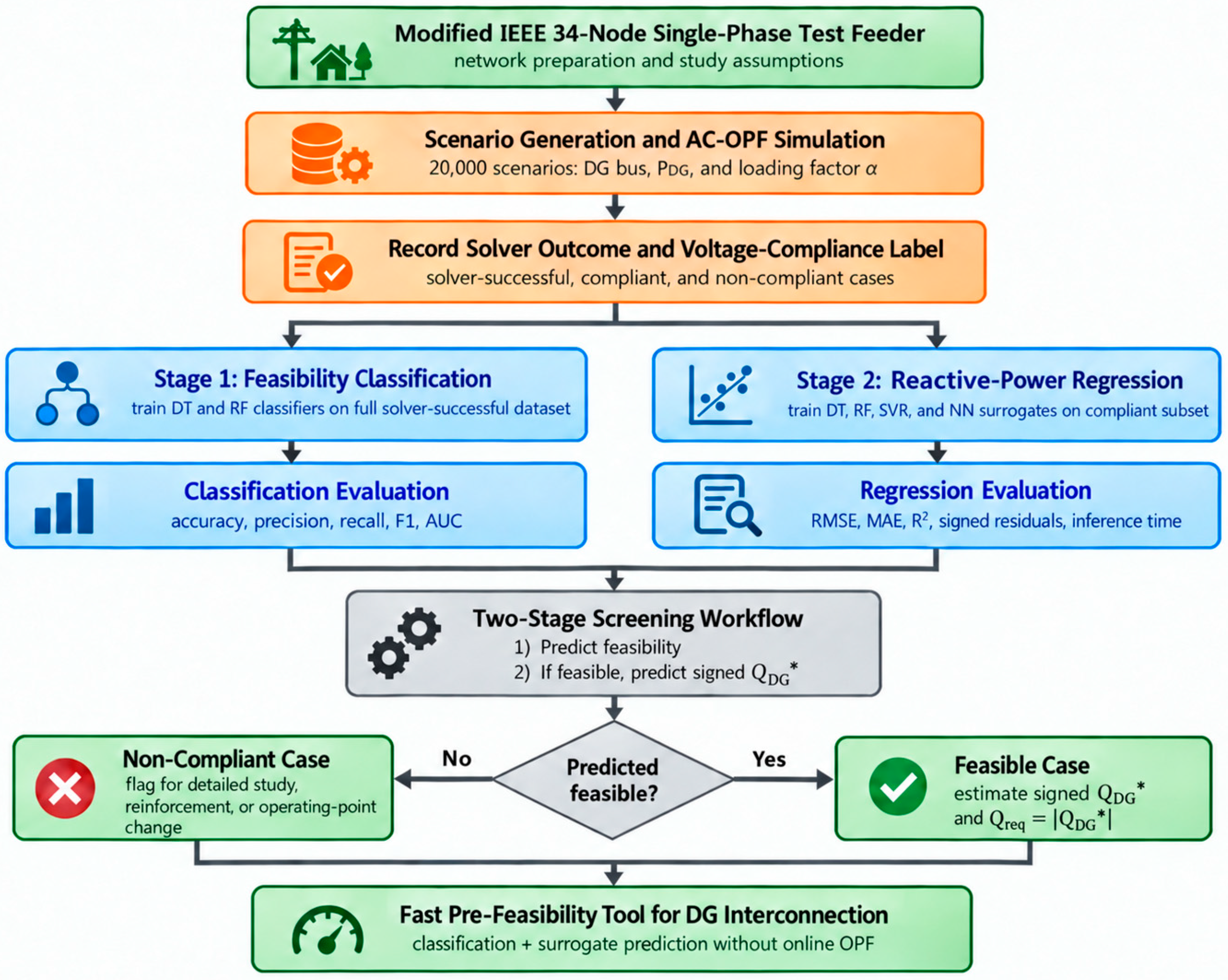
The framework combines physics-based optimization and data-driven learning in five elements: network modeling, AC–OPF formulation, scenario sampling, Stage-1 feasibility classification, and Stage-2 reactive-power regression, as summarized conceptually in Figure 1. For each scenario, the OPF inputs are the DG connection bus, fixed active-power injection P_DG, and feeder loading factor α. The OPF decision variables are bus voltage magnitudes and angles together with generator active/reactive powers; recorded outputs include the signed optimal DG reactive-power setpoint Q_DG*, voltage extrema, solver status, engineering-compliance label, and solve time. Both ML stages receive DG location encoded as 21 categorical one-hot indicators together with P_DG and α. Stage 1 predicts the binary compliance label, whereas Stage 2 predicts the signed Q_DG* setpoint only for scenarios labeled feasible.
Figure 1.
Overall methodology for reactive-power-conditioned hosting capacity assessment using OPF-based dataset generation and machine learning surrogate models. The superscript * denotes the optimal OPF reactive-power setpoint. Abbreviations: DG, distributed generation; AC–OPF, AC optimal power flow; DT, decision tree; RF, random forest; SVR, support vector regression; NN, neural network; AUC, area under the receiver operating characteristic curve; RMSE, root mean square error; MAE, mean absolute error. P_DG, DG active power; α, feeder loading factor; Q_DG*, optimal signed DG reactive-power setpoint; Q_req, required reactive-power magnitude. The superscript * denotes the optimal OPF-derived setpoint.
2.1. Distribution Network Modeling
The test system is based on the IEEE 34-node radial feeder [15,16]. The radial structure is also consistent with branch-flow formulations commonly used for distribution networks [17]. Only phase A is modeled and loads are represented as constant PQ injections. Voltage regulators, shunt capacitors, and step-down transformers are deliberately removed so that their discrete or controlled voltage-support actions do not mask the intrinsic sensitivity of feeder voltage to DG location, active-power injection, and reactive-power exchange. The resulting model is therefore a controlled passive-feeder benchmark, not a direct replica of a utility feeder. Line impedances are obtained from the IEEE conductor-configuration data and physical line lengths. For a line connecting buses i and j,
where and are resistance and reactance per mile and is the line length in feet. The bus admittance matrix is assembled using the standard nodal formulation [18]; its real and imaginary parts define the conductance matrix and susceptance matrix .
2.2. AC Optimal Power Flow Formulation
The AC–OPF determines the minimum-magnitude reactive-power setpoint required from a candidate DG for a specified operating condition while prioritizing the engineering voltage criterion. Decision variables are voltage magnitudes V, voltage angles θ, and generator active/reactive powers P_g and Q_g. The sign convention follows the nodal balance equations: Q_DG > 0 denotes reactive-power injection into the feeder, whereas Q_DG < 0 denotes reactive-power absorption. The regression target is the signed optimum Q_DG*; when only the required magnitude is discussed, Q_req = |Q_DG*|.
2.2.1. Power Balance Constraints
For each bus ,
2.2.2. Voltage and Generator Constraints
Voltage magnitudes satisfy
To keep severe radial-feeder cases numerically solvable, voltage variables use broad numerical bounds of 0.70–1.15 p.u.; engineering compliance is assessed against 0.95–1.05 p.u. using non-negative voltage-violation slack variables that are strongly penalized in the objective. The 0.95–1.05 p.u. band is used here as an engineering screening criterion for the benchmark and is not intended to reproduce all requirements of IEEE 1547 or a specific local interconnection code. The candidate DG has |Q_DG| ≤ 0.5 MVAr and S_DG = 2.0 MVA, which is compatible with the sampled active-power range up to 1.8 MW:
2.2.3. Objective Function
The revised objective first minimizes violations of the 0.95–1.05 p.u. engineering band and, when zero violation is attainable, minimizes the magnitude of the signed DG reactive-power setpoint:
min M Σi(si− + si+) + (Q_DG/Q_max)2 + w_s(P_slack2 + Q_slack2)
Here, si− and si+ quantify lower- and upper-voltage-band violations, M is a large penalty coefficient, and w_s is a small slack-bus regularization weight. The optimized quantity Q_DG* is a signed setpoint: positive values denote reactive-power injection and negative values denote absorption. When only inverter capability magnitude is required, Q_req = |Q_DG*| is obtained as a derived quantity; Q_req is not the regression target. Cases that cannot attain the engineering band within the modeled DG capability are retained as non-compliant screening outcomes rather than being assigned a regression target. IPOPT is used to obtain locally optimal NLP solutions; solver termination is checked explicitly, and failed cases are excluded from ML training. As with any nonconvex AC–OPF, the solution can remain sensitive to initialization and network-parameter assumptions, so the OPF labels should be interpreted within the stated benchmark model.
2.3. Scenario Sampling and Dataset Generation
A total of 20,000 scenarios are generated. The DG connection bus is sampled uniformly from buses 2–22. For P_DG, 70% of samples are drawn uniformly from 0 to 0.8 MW and 30% from 0.8 to 1.8 MW. For the loading factor α, 60% of samples are drawn uniformly from 0.70 to 0.95, 30% from 0.95 to 1.10, and 10% from 0.45 to 0.70. In the revised dataset, all nodal loads are scaled deterministically by α; no additional unobserved bus-by-bus random perturbations are applied, thereby removing hidden ambiguity between the surrogate inputs and the OPF target:
P_d,i = α P_d,i0, Q_d,i = α Q_d,i0
The solver successfully terminates for 19,930 of the 20,000 generated scenarios (99.65%). Among the solver-successful cases, 12,300 (61.72%; 61.50% of all generated cases) achieve the 0.95–1.05 p.u. engineering band within the DG reactive-power and apparent-power limits, whereas 7630 are non-compliant. The 19,930 solver-successful cases are used for Stage-1 classification; only the 12,300 compliant cases form the Stage-2 regression dataset. The 70 solver-failed cases are recorded separately and excluded from ML training. For each successful case, Q_DG*, |Q_DG*|, voltage extrema, compliance status, and OPF solution time are stored.
For reproducibility, scenario sampling uses the fixed random seed 20260911. The OPF is solved using Pyomo 6.5 with IPOPT 3.14.5 using the stated model and default solver tolerances; voltage variables use the broad numerical envelope 0.70–1.15 p.u., while 0.95–1.05 p.u. defines the engineering-compliance label. The DG limits are |Q_DG| ≤ 0.5 MVAr and S_DG = 2.0 MVA; the soft-voltage penalty and slack-bus regularization weights are M = 106 and w_s = 10−3, respectively. The full dataset records scenario ID, DG bus, P_DG, α, solver termination/status, compliance label, signed Q_DG*, reactive-power magnitude, voltage extrema, and solve time. Both ML stages are implemented in MATLAB R2023a and use 10-fold cross-validation with the same fixed seed; Stage 1 uses stratified folds. The complete datasets and Python/MATLAB scripts are supplied as the Supplementary Materials.
2.4. Machine Learning Models
Machine learning is used in two distinct roles. Stage 1 is a binary feasibility classifier trained on all 19,930 solver-successful scenarios, with the 0.95–1.05 p.u. compliance label as the target. Decision-tree (DT) and random-forest (RF) classifiers are evaluated using stratified 10-fold cross-validation. Stage 2 is a regression surrogate trained only on the 12,300 compliant scenarios. Its target is the signed optimal reactive-power setpoint Q_DG*, and the regression mapping is
where z_bus denotes the 21-element one-hot representation of DG location. Thus, Q_req = |Q_DG*| is only a post-processed magnitude and is not the variable learned by the regression models. Stage-2 regression is evaluated with DT, RF, SVR, and feedforward NN models using 10-fold cross-validation. P_DG and α are the two continuous inputs, giving 23 features in total together with z_bus. Only the continuous inputs are standardized fold-by-fold for SVR and NN. Out-of-fold predictions are evaluated using MSE, RMSE, R2, MAE, mean and median signed residuals (Q_pred − Q_OPF), and the 95th percentile of absolute error. Inference time is measured on held-out fold batches after a warm-up prediction and normalized per sample. The principal regression hyperparameters are summarized in Table 1.
Table 1.
Main hyperparameters of the evaluated ML regression models.
2.5. Operational Two-Stage Screening Procedure
For a new candidate scenario x = (z_bus, P_DG, α), Stage 1 first predicts whether the available inverter capability can satisfy the 0.95–1.05 p.u. engineering voltage criterion. If the case is classified as non-compliant, the regression surrogate is not applied; instead, the request is flagged for detailed OPF/interconnection analysis, a different inverter capability, operating-point modification, or network reinforcement. If the case is classified as feasible, Stage 2 estimates the signed setpoint Q_DG*. Formal interconnection decisions must still be verified with the detailed electrical model because the classifier is a screening surrogate rather than a protection against all false-feasible classifications.
3. Results and Discussion
3.1. Two-Stage Screening Performance
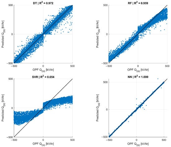
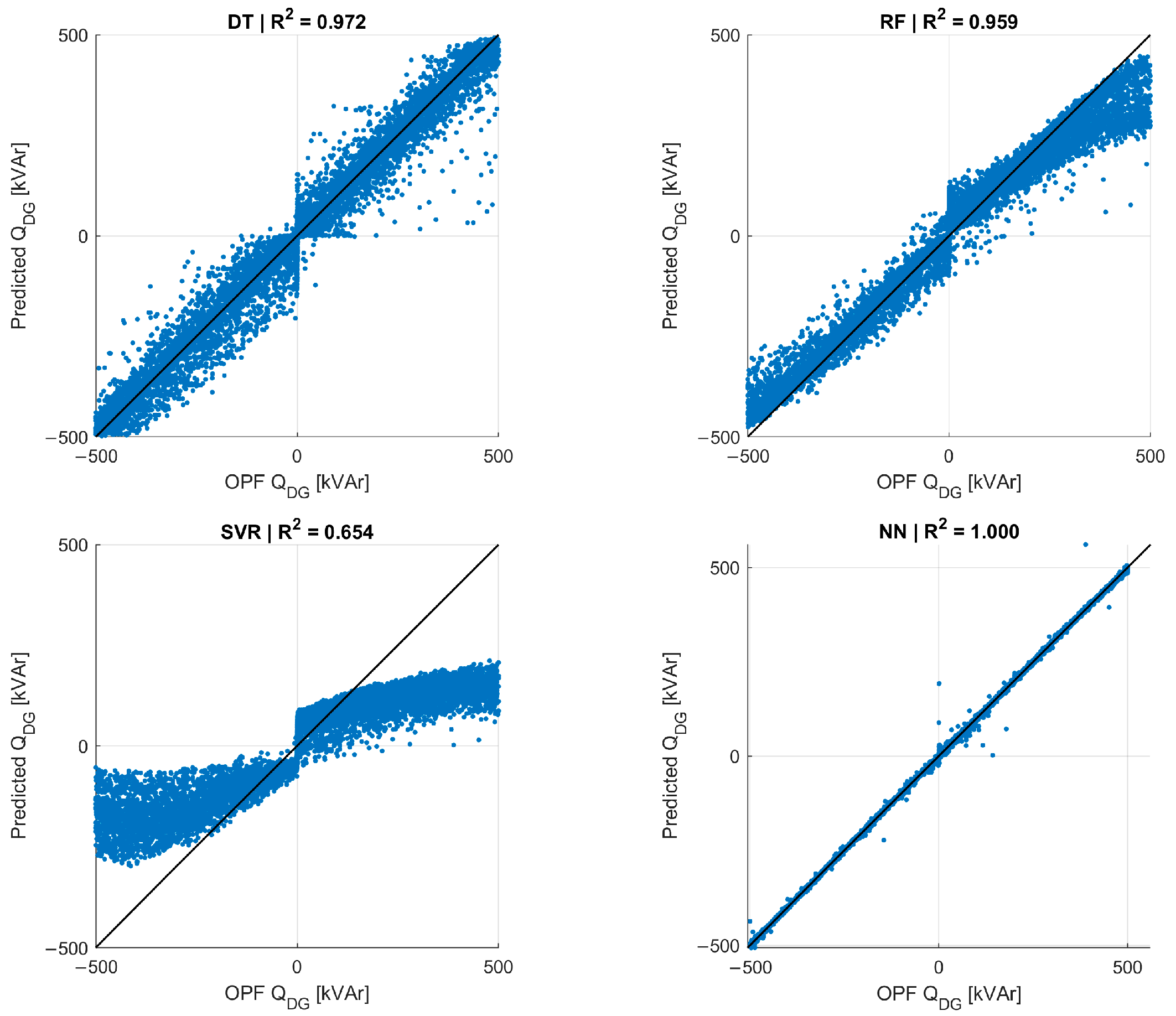
Stage 1 is evaluated on all 19,930 solver-successful scenarios (12,300 feasible and 7630 non-compliant). The DT classifier achieves 97.41% accuracy, 97.75% precision, 98.06% recall, 96.37% specificity, F1 = 97.91%, balanced accuracy = 97.21%, and ROC-AUC = 0.9908. At the default classification threshold, its out-of-fold confusion counts are 12,061 true positives, 7353 true negatives, 277 false positives, and 239 false negatives. RF reaches ROC-AUC = 0.9938 but has lower threshold-based performance (95.32% accuracy; F1 = 96.22%) and substantially higher inference time, so DT is retained as the Stage-1 screening classifier. Conditional on feasibility, Table 2 reports Stage-2 regression performance. The NN provides the highest accuracy by a clear margin, with R2 = 0.9996, RMSE = 4.745 kVAr, and MAE = 1.964 kVAr. DT remains accurate and interpretable (R2 = 0.9719; RMSE = 37.612 kVAr), RF gives R2 = 0.9587, and SVR gives R2 = 0.6540. The NN mean signed residual is 0.005 kVAr and the DT mean signed residual is −1.328 kVAr, both small relative to the ±500 kVAr target range.
Table 2.
Performance of ML regression models using K-fold cross-validation (K = 10).
Because model training is performed offline, training time is not used as the primary argument for online applicability. The mean OPF solution time for the compliant cases is 0.1456 s per scenario (median 0.1200 s; 95th percentile 0.2247 s), whereas batched surrogate inference requires approximately 0.504 μs/sample for NN, 1.106 μs/sample for DT, 114.9 μs/sample for RF, and 141.0 μs/sample for SVR. Thus, the revised evidence supports several orders of magnitude reduction in per-scenario evaluation time. NN is preferred when predictive accuracy is paramount, while DT remains attractive when transparent rule-based interpretation is desired.
3.2. Parity Analysis
Figure 2 compares OPF-derived signed Q_DG* values and out-of-fold ML predictions. NN predictions remain tightly concentrated around the ideal diagonal over the full −500 to +500 kVAr range. DT and RF reproduce the overall mapping with larger local deviations, whereas SVR shows pronounced compression toward the center of the target range.
Figure 2.
Parity plots of OPF-derived versus out-of-fold predicted signed DG reactive-power setpoints for the four surrogate models. DG location is encoded categorically; the solid line denotes the ideal relationship.
3.3. Three-Dimensional Analysis
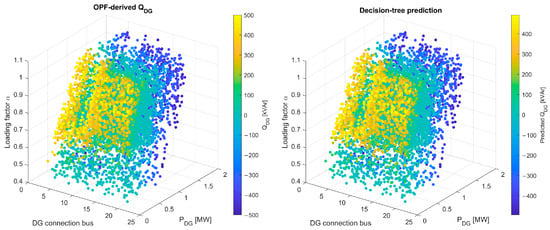
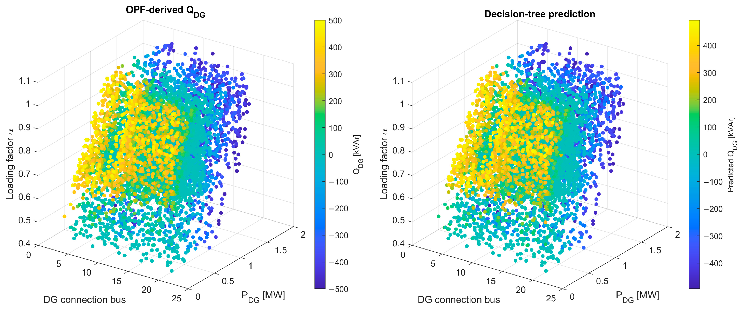
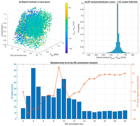
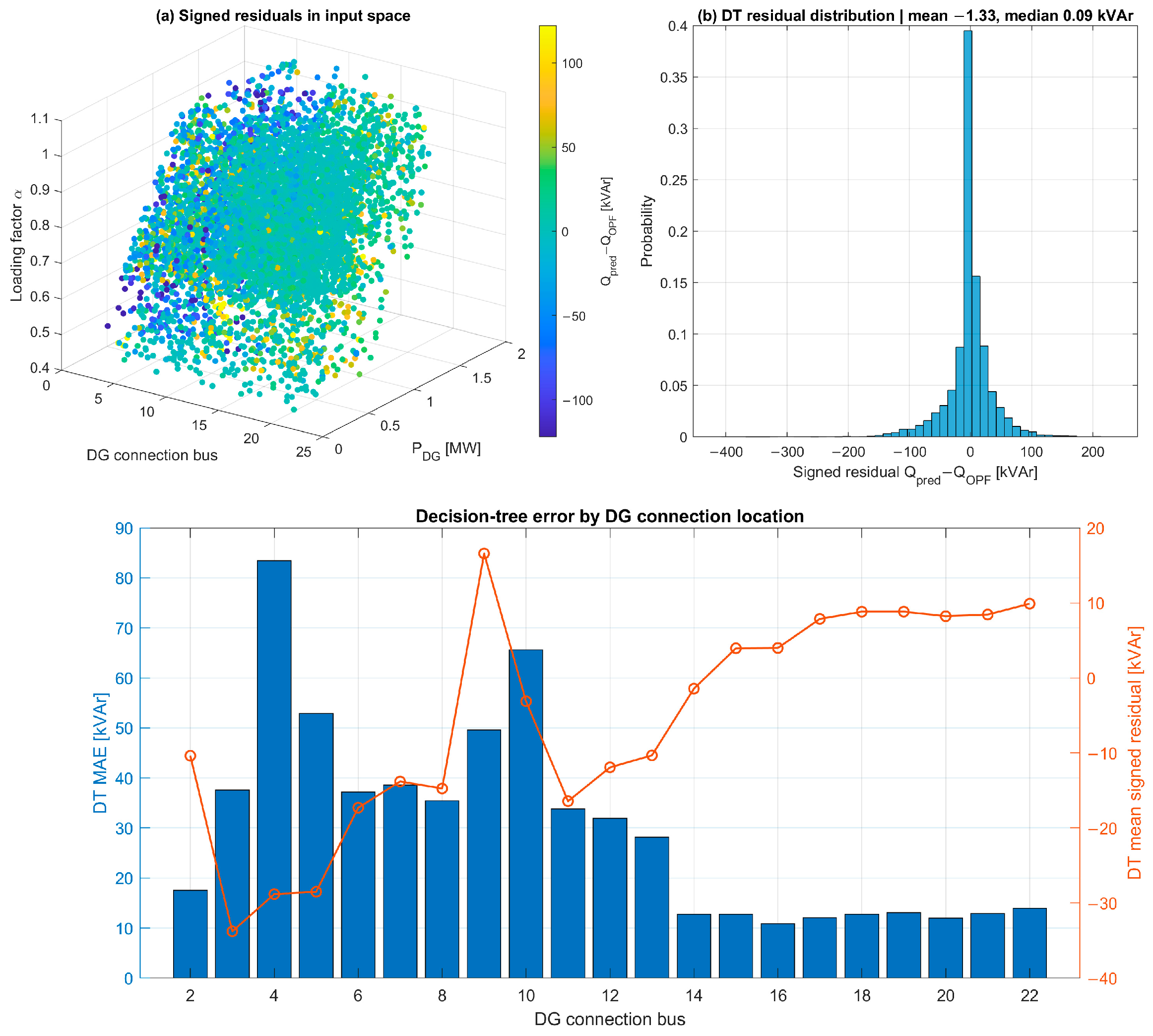
Figure 3 and Figure 4 examine DT behavior in the input space and through signed residuals. The predicted landscape broadly follows the OPF-derived reactive-power pattern across DG location, active-power injection, and loading factor. Unlike the original absolute-error plot, Figure 4 uses the signed residual e_Q = Q_pred − Q_OPF. The overall DT residual distribution has a mean of −1.33 kVAr and a median of 0.09 kVAr, providing quantitative evidence of small global bias. A separate bus-location analysis shows that error is not spatially uniform: DT MAE is approximately 11–14 kVAr for many downstream buses but is larger at several upstream/intermediate locations. Buses 2–4 contain only 3, 8, and 37 compliant samples, respectively, so their bus-specific statistics are not interpreted as robust generalization estimates.
Figure 3.
Three-dimensional comparison of the signed reactive-power setpoint across DG connection bus, active-power injection P_DG, and loading factor α: left, OPF-derived reference; right, decision-tree prediction.
Figure 4.
Decision-tree residual analysis. (Top left): signed residuals (Q_pred − Q_OPF) across the input space. (Top right): residual distribution with mean and median values. (Bottom): MAE and mean signed residual by DG connection bus, providing a location-specific error assessment. In the (top-left) panel, color denotes the signed residual according to the color bar; in the (bottom) panel, bars denote MAE and the line denotes mean signed residual.
3.4. Engineering Implications and Limitations
The revised framework makes the screening logic explicit. Stage 1 first separates likely voltage-compliant and non-compliant cases, and Stage 2 estimates Q_DG* only for cases classified as feasible. This avoids applying the regression model outside the population on which it was trained. The DT classifier is highly accurate but not perfect: 277 of 7630 truly non-compliant out-of-fold cases are labeled feasible, corresponding to 96.37% specificity. Therefore, the method is intended for preliminary prioritization rather than automatic interconnection approval; borderline or formally submitted cases should still be verified using the detailed electrical model. For feasible cases, surrogate inference is measured in microseconds per scenario, whereas the reference OPF requires approximately 0.146 s on average. The broader scope remains intentionally limited to one simplified single-phase feeder with removed voltage-control devices, fixed network parameters, one DG capability model, and deterministic load scaling through α. External validation on detailed unbalanced feeders is required before operational deployment.
4. Conclusions
This paper evaluated a two-stage OPF–ML framework for rapid DG pre-feasibility screening on a controlled single-feeder benchmark. A revised set of 20,000 OPF scenarios was generated over 21 candidate buses, P_DG up to 1.8 MW, and loading factors from 0.45 to 1.10. Of these, 19,930 were solved successfully; 12,300 were voltage-compliant and 7630 were non-compliant. Stage 1 uses a DT classifier to separate these outcomes and achieved 97.41% accuracy, 96.37% specificity, F1 = 97.91%, and ROC-AUC = 0.9908 under stratified 10-fold cross-validation. Stage 2 is applied only to cases classified as feasible and predicts the signed Q_DG* setpoint; the NN achieved R2 = 0.9996, RMSE = 4.745 kVAr, and MAE = 1.964 kVAr. Categorical encoding of DG location and deterministic loading through α make the surrogate inputs explicit, while the supplied dataset and code improve reproducibility. Because Stage 1 can still produce false-feasible classifications and the feeder model is simplified, the framework should be interpreted as a fast screening aid that complements rather than replaces detailed three-phase interconnection studies.
Supplementary Materials
The following supporting information can be downloaded at: https://www.mdpi.com/article/10.3390/engproc2026158027/s1, File S1: complete 20,000-scenario OPF dataset; File S2: 12,300-case compliant regression subset; File S3: Python notebook for OPF scenario generation (Pyomo 6.5, IPOPT 3.14.5); File S4: MATLAB R2023a script for Stage-2 regression training; File S5: MATLAB R2023a script for Stage-1 feasibility classification; File S6: Stage-2 regression metrics; File S7: Stage-1 classifier metrics; File S8: Stage-1 out-of-fold predictions; File S9: Stage-1 metrics by DG bus. The supporting files provided with this article include the complete 20,000-scenario OPF dataset, the 12,300-case compliant regression subset, the Python notebook used for OPF scenario generation, the MATLAB scripts used for Stage-1 feasibility classification and Stage-2 regression, and summary output files documenting the reported performance metrics.
Author Contributions
Conceptualization, E.N., L.M., G.S.P., J.R. and J.M.-A.; methodology, E.N.; software, E.N.; validation, E.N., L.M., G.S.P., J.R. and J.M.-A.; formal analysis, E.N.; investigation, E.N.; data curation, E.N.; writing—original draft preparation, E.N.; writing—review and editing, E.N., L.M., G.S.P., J.R. and J.M.-A.; visualization, E.N.; project administration, E.N. All authors have read and agreed to the published version of the manuscript.
Funding
This research was supported by Escuela Politécnica Nacional (EPN), Quito, Ecuador, through its Doctoral Program in Electrical Engineering, which provided institutional and financial support for the development of this work. No grant number was assigned to this institutional support.
Institutional Review Board Statement
Not applicable.
Informed Consent Statement
Not applicable.
Data Availability Statement
The network data were derived from the publicly available IEEE 34-Node Test Feeder at https://site.ieee.org/pes-testfeeders/resources/ (accessed on 20 January 2026). The complete OPF-generated dataset, compliant regression subset, and Python/MATLAB analysis scripts used in this study are provided as Supplementary Materials to enable reproduction of the reported scenario generation, two-stage ML training, and performance evaluation.
Acknowledgments
The authors would like to thank Escuela Politécnica Nacional (EPN), Quito, Ecuador, for the academic, technical, and institutional support provided for the development of this research. During manuscript preparation, ChatGPT (OpenAI, GPT-5.6 Sol) was used solely for language editing, readability improvement, and document formatting; it was not used to generate OPF/ML numerical results or determine the scientific conclusions. The authors reviewed and edited all assisted text and take full responsibility for the publication content.
Conflicts of Interest
The authors declare no conflicts of interest. The funders had no role in the design of the study; in the collection, analyses, or interpretation of data; in the writing of the manuscript; or in the decision to publish the results.
Abbreviations
The following abbreviations are used in this manuscript:
| DG | Distributed Generation |
| OPF | Optimal Power Flow |
| ML | Machine Learning |
| DT | Decision Tree |
| RF | Random Forest |
| SVR | Support Vector Regression |
| NN | Neural Network |
| RMSE | Root Mean Square Error |
| MSE | Mean Squared Error |
| pu | Per Unit |
References
- Electric Power Research Institute (EPRI). Impact Factors, Methods, and Considerations for Calculating and Applying Hosting Capacity; EPRI: Palo Alto, CA, USA, 2018; No. 3002011009; Available online: https://www.epri.com/research/products/000000003002011009 (accessed on 20 January 2026).
- Bollen, M.H.J.; Hassan, F. Integration of Distributed Generation in the Power System; Wiley-IEEE Press: Hoboken, NJ, USA, 2011. [Google Scholar] [CrossRef] [Scilit]
- IEC 61727:2004; Photovoltaic (PV) Systems—Characteristics of the Utility Interface. International Electrotechnical Commission (IEC): Geneva, Switzerland, 2004.
- IEEE Std 1547-2018; IEEE Standard for Interconnection and Interoperability of Distributed Energy Resources with Associated Electric Power Systems Interfaces. IEEE: New York, NY, USA, 2018.
- Turitsyn, K.; Šulc, P.; Backhaus, S.; Chertkov, M. Options for Control of Reactive Power by Distributed Photovoltaic Generators. Proc. IEEE 2011, 99, 1063–1073. [Google Scholar] [CrossRef] [Scilit]
- Kryonidis, G.C.; Malamaki, K.N.D.; Gkavanoudis, S.I.; Oureilidis, K.; Kontis, E.O.; Mauricio, J.M.; Maza-Ortega, J.M.; Demoulias, C.S. Distributed Reactive Power Control Scheme for the Voltage Regulation of Unbalanced LV Grids. IEEE Trans. Sustain. Energy 2021, 12, 1301–1310. [Google Scholar] [CrossRef] [Scilit]
- Ayaz, M.S.; Malekpour, M.; Azizipanah-Abarghooee, R.; Terzija, V. Local Photovoltaic Reactive Power Controller for Increasing Active Distribution Networks Hosting Capacity. IET Gener. Transm. Distrib. 2020, 14, 5152–5162. [Google Scholar] [CrossRef] [Scilit]
- Hu, X.; Liu, Z.-W.; Wen, G.; Yu, X.; Liu, C. Voltage Control for Distribution Networks via Coordinated Regulation of Active and Reactive Power of DGs. IEEE Trans. Smart Grid 2020, 11, 4017–4031. [Google Scholar] [CrossRef] [Scilit]
- Momoh, J.A.; El-Hawary, M.E.; Adapa, R. A Review of Selected Optimal Power Flow Literature to 1993. Part I: Nonlinear and Quadratic Programming Approaches. IEEE Trans. Power Syst. 1999, 14, 96–104. [Google Scholar] [CrossRef] [Scilit]
- Frank, S.; Steponavice, I.; Rebennack, S. Optimal Power Flow: A Bibliographic Survey I. Formulations and Deterministic Methods. Energy Syst. 2012, 3, 221–258. [Google Scholar] [CrossRef] [Scilit]
- Novoa, E.; Cepeda, J. Reactive Power Support from Distributed Generation to Maximize Active Power Injection in Distribution Networks. Eng. Proc. 2025, 115, 6. [Google Scholar] [CrossRef] [Scilit]
- Hastie, T.; Tibshirani, R.; Friedman, J. The Elements of Statistical Learning: Data Mining, Inference, and Prediction, 2nd ed.; Springer: New York, NY, USA, 2009. [Google Scholar] [CrossRef]
- Bishop, C.M. Pattern Recognition and Machine Learning; Springer: New York, NY, USA, 2006. [Google Scholar]
- Goodfellow, I.; Bengio, Y.; Courville, A. Deep Learning; MIT Press: Cambridge, MA, USA, 2016. [Google Scholar]
- Kersting, W.H. Radial Distribution Test Feeders. IEEE Trans. Power Syst. 1991, 6, 975–985. [Google Scholar] [CrossRef] [Scilit]
- IEEE PES Distribution System Analysis Subcommittee. IEEE 34-Node Test Feeder Data. 2018. Available online: https://site.ieee.org/pes-testfeeders/resources/ (accessed on 20 January 2026).
- Farivar, M.; Low, S.H. Branch Flow Model: Relaxations and Convexification—Part I. IEEE Trans. Power Syst. 2013, 28, 2554–2564. [Google Scholar] [CrossRef] [Scilit]
- Grainger, J.J.; Stevenson, W.D. Power System Analysis; McGraw-Hill: New York, NY, USA, 1994. [Google Scholar]

Disclaimer/Publisher’s Note: The statements, opinions and data contained in all publications are solely those of the individual author(s) and contributor(s) and not of MDPI and/or the editor(s). MDPI and/or the editor(s) disclaim responsibility for any injury to people or property resulting from any ideas, methods, instructions or products referred to in the content. |
© 2026 by the authors. Licensee MDPI, Basel, Switzerland. This article is an open access article distributed under the terms and conditions of the Creative Commons Attribution (CC BY) license.