Forecasting MBTA Transit Dynamics: A Performance Benchmarking of Statistical and Machine Learning Models ^†

Abstract

The Massachusetts Bay Transportation Authority (MBTA) is the main public transit provider in Boston, operating multiple means of transport, including trains, subways, and buses. However, the system often experiences delays and fluctuations in ridership, which undermine efficiency and passenger satisfaction. To better understand this phenomenon, this paper compares the performance of existing and novel methods to determine the best approach for predicting gated station entries in the subway system (a proxy for subway usage) and the number of delays across the overall MBTA system. To do so, this research considers factors that affect public transportation, such as day of the week, season, pressure, wind speed, average temperature, and precipitation. This paper evaluates the performance of 10 statistical and machine learning models on predicting next-day subway usage. For predicting delay count, the number of models is extended to 11 per day by introducing a self-exciting point process model, representing a unique application of a point-process framework for MBTA delay modeling. This research involves experimenting with the selective inclusion of features to determine feature importance and testing model accuracy via Root Mean Squared Error (RMSE). Remarkably, it is found that providing either day-of-week or season data yields a greater benefit to predictive accuracy than weather data; in fact, providing weather data generally worsens performance, suggesting a tendency for models to overfit.

1. Introduction

Public transit forecasting has become increasingly important as cities grow denser and more transportation facilities are developed. Thus, understanding and predicting fluctuations in transit demand is vital for efficient operation, sustainability, and resource allocation. Public transportation is heavily influenced by many factors, with weather conditions playing a crucial role. Understanding how weather impacts the transit system can lead to better planning and ridership satisfaction in the future. Many studies have explored this field and found that weather factors, such as temperature, precipitation, wind speed, and other conditions, affect ridership patterns [1,2,3,4]. For instance, Singhal et al., Guo et al., and Wei et al. studied the relationship between urban transit ridership and weather variations in New York City, Chicago, and Brisbane, through which all of the studies showed some sort of impact of weather on ridership; generally, bad weather tends to reduce ridership. Studying the impact of these same factors in Boston would prove rewarding as Boston’s public transit system functions similarly to Chicago and New York City.

The Massachusetts Bay Transportation Authority (MBTA), serving the Boston area, is similarly vulnerable to fluctuating weather conditions. Over 800,000 people use the MBTA system each month, making it the third-largest public transit system in the United States [5,6]. Furthermore, Boston is the seventh most densely populated metropolitan area in the United States, making transportation infrastructure a challenging endeavor for city planners [7]. Public transportation is notoriously unreliable in the United States due to many factors that influence its performance.

Currently, these factors create widespread issues with consumer transportation and reliability, leading many to deviate from public transit. MassINC, a polling group, conducted a survey to determine customer satisfaction with MBTA services. They found that, with the commuter rail, 46% of people rate the system as excellent, compared with 35% who rate bus services as at least good, and 28% who feel similarly about the subway and trolley network [7]. When large-magnitude changes occur, the MBTA schedule becomes largely unreliable, so it is vital that the city of Boston knows how many passengers to expect on its system, and that passengers know in advance when their subways are delayed. Thus, this paper aims to analyze the impacts of weather, season, and day of the week on subway ridership volume and delays.

Despite growing interest in public transit prediction, relatively few studies have jointly explored ridership and delay formation, nor have they systematically examined the relative importance of calendar versus environmental variables in a multi-model setting. This study examines the impact of calendar factors (day of the week, season) and weather conditions (pressure, average temperature, wind speed, precipitation) on daily gated-station entries (as a proxy for subway usage) and system-wide delay counts in the MBTA. The MBTA operates subway, commuter rail, and bus services throughout the Boston metropolitan area. Eleven statistical and machine learning models are implemented and evaluated, including a novel self-exciting point-process model for predicting delay events. Models used include Random Forest Regression, Linear Regression, Ridge Regression, Lasso Regression, Gradient Boost Regression, Linear Support Vector Regression, Multilayer Perceptrons, K-Nearest-Neighbor Regression, Moving Averages, and Poisson Regression. The outcomes from this analysis can help the MBTA and other transit authorities in future planning, investments, and the resilience of transportation networks. A public, one-click reproducible GitHub (version 3.18) repository for Mac has also been built to facilitate reproducibility.

A narrative literature review was conducted in July 2025, using English-language academic papers published in peer-reviewed journals or conference proceedings. The search began with keywords such as “predicting public transit delays,” “predicting passenger ridership,” and “train prediction.” Initially, 200+ related papers on this topic were found using ResearchRabbit. Using these papers, the literature review was divided into two parts: subway delays and ridership predictions.

Past literature has focused on predicting transit delays between stops (in response to [8]), which is effective at informing passengers whether the approaching train, bus, or subway will be delayed; however, this approach has limited real-world practicality. Tracking every bus, train, and subway in a city—or even a state—would take enormous computational power and make the results hard to access. In response to this, our research focuses on aggregate daily subway delays, which require less computing power and keep both the local transit authority (in this case, the MBTA) and passengers realistically informed of overall conditions.

Several studies recognize the myriad of factors that influence delay prediction. Recent work by Zhang et al. [8] extends the delay-prediction field of research beyond the usual single-equation solution. Instead of using a huge model for an entire route, they treat each stop as a separate regression equation and estimate the whole system with a seemingly unrelated regression equations (SURE) estimator, which can catch neglected correlations among residuals, such as driver behavior or traffic shocks. Using six months of bus operation data from Stockholm, Sweden, the stop-specific SURE model achieved RMSEs of 30–42 s and $R^2$ values above 0.92, outperforming an ordinary least squares (OLS) model while remaining computationally inexpensive. Zhang et al. highlight that bus operational factors, such as upstream delays and dwell times, are the primary causes of delays, whereas calendar and weather factors have weaker effects.

Srivastava et al. [9] introduce the first rail-specific delay model that combines causal inference with machine learning uplift modeling. They used a 1.5-million-trip New Jersey Transit dataset spanning 2018–2020, and each candidate covariate (such as stop sequence and actual time) was treated as a treatment. The Average Treatment Effect (ATE) and Individual Treatment Effect (ITE) were estimated using an Uplift Tree classifier, which allows for understanding why a forecast changes. They found that the stop sequence (ATE roughly equals 0.98) and actual departure/arrival times (ATE roughly equals 0.97) dominated the formation of delays, more so than weather or any other factors. After retraining with only the most influential causal features, the uplift model still achieved a 95.6% accuracy, outperforming XGBoost, Random Forest, and Support Vector Machine (SVM) on the same dataset.

Deep learning is also a competitive alternative for ridership forecasting. Demonstrated by Wang et al. [10], a DST-TransitNet model was proposed, a dynamic spatio-temporal deep learning model that predicts ridership at the station level. DST-TransitNet employs a hybrid deep learning architecture that integrates Graph Neural Networks (GNNs), Graph Attention Networks (GATs), and Gated Recurrent Units (GRUs) to dynamically model both spatial and temporal features in the data. Unlike previous models that treat stop-to-stop relationships as static, DST-TransitNet calculates dynamic edge weights based on recent ridership, enabling the model to capture changing correlations between stations throughout the day. This is particularly useful when there is fluctuating data due to events such as COVID-19 or protests. The model was tested on the Bogota Rapid Transit (BRT) system in Bogota, Colombia, using over five years of 15-minute interval data across 147 stations. DST-TransitNet significantly outperforms state-of-the-art models like LSTM, iTransformer, and DLinear.

Similarly, He et al. [11] developed a Multi-Graph Convolutional-Recurrent Neural Network (MGC-RNN) that incorporates spatial and temporal dependencies and other complex factors. They tackled short-term passenger flow by combining five complementary graphs (network distance, Point-Of-Interest (POI) correlation, network structure correlation, operational information correlation, and recent flow correlation) with a sequence-to-sequence (seq2seq) LSTM encoder–decoder. The model handles both static and time-varying inter-station correlations. Applied to 118 stations on the Shenzhen Metro in China, the results showed that holiday, day of the week, and weather variables did not significantly affect the outputs, whereas graph features and recent activity dominated the outputs.

Tiong et al., consistent with other authors, claim that factors such as crew schedule, rolling stock circulation, infrastructure data, passenger data, weather, peak hours, calendar features, roadwork, and maintenance activities can affect train delays [12]. There are two main areas for improvement that can be identified from this. Firstly, collecting such a vast amount of data is resource-intensive, making it both costly and time-consuming. As a result, our project focuses on limiting the number of inputs to make it more realistic and practical. Secondly, existing research overlooks the day of the week as a major factor in delay prediction, which our research finds to be strongly correlated. Most existing literature examines more “common sense” factors by surveying transportation experts [13,14]. This would help organizations like the MBTA do their work with minimal cost as the day of the week is easily accessible.

Regarding daily passenger ridership in the MBTA system, the literature has explored various methods for predicting it. There is academic literature that focuses on using ARIMA (Autoregressive Integrated Moving Average), SVM (Support Vector Machine), a probabilistic approach (utilizing statistical models), and a Deep Learning/Machine Learning approach [15]. Past literature has focused on Deep Learning and ML models, which, on average, outperform traditional time series models (which focus on a dependent variable changing over time) [15]. More recent literature focuses on more innovative approaches to this prediction problem, such as using attention-based models [16]. Other papers use image analysis of short-term metro traffic as a unique approach to attempt short-term forecasting. Similar to delay prediction, most literature overlooks the day of the week as a critical variable in predicting passenger flow, which our research highlights. In addition, literature does not focus on the models that are the target of our investigation [16].

The remainder of the paper is organized as follows: Section 2 presents the study’s methodology, including a discussion of the data analysis and the model type. Section 3 discusses the performance of the various models studied and benchmarks them against each other. Finally, Section 4 presents a summary of key findings and avenues for further research.

2. Methodology

2.1. Statistical Analysis of the Data

The data used for this article came from Meteostat and the Massachusetts Bay Transportation Authority (MBTA). Meteostat provided the weather data for Boston Logan International Airport, which was used as a proxy for Boston weather during the target time period. The dataset included pressure, wind speed, average temperature, and precipitation.

The MBTA provided all the public transit-related datasets. The “MBTA Service Alerts” dataset [17] provided delay data, while the “MBTA Gated Station Entries” dataset [18] provided ridership data. The CSV file with delay data spans from 1 January 2019 to 29 July 2023. After cleaning and computing daily aggregations for each metric, there are 1671 entries. Though the dataset is classified as “deprecated” by the MBTA, it remains highly accurate and relevant to future regression in 2025 and beyond.

The gated station entry dataset spans from 1 January 2014, to 30 June 2025, and contains 4199 entries.

After data wrangling, both datasets were processed into 36-column datasets that contain all necessary data (day of the week, weather, season, etc.). Processed datasets can be found in the corresponding section of our Github repository, https://github.com/icoder178/mbta-prediction-models/tree/main/data (accessed on 21 April 2026).

2.2. ML Model Comparison

Our comparative study evaluates how well various machine-learning models [19,20] predict two next-day outcomes for the MBTA system: (i) the total number of recorded service delays (Delay task) and (ii) the total number of gated-station entries (GSE task). For each calendar day, a five-day sliding window is constructed that includes the target series itself and optional covariates. These optional inputs come from three conceptually distinct groups: day-of-week indicators, seasonal indicators, and four basic weather measurements (pressure, wind speed, precipitation, temperature). After flattening the 5 × k matrix to a single vector, a fixed-length feature tensor suitable for any scikit-learn regressor is created.

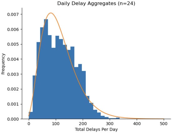
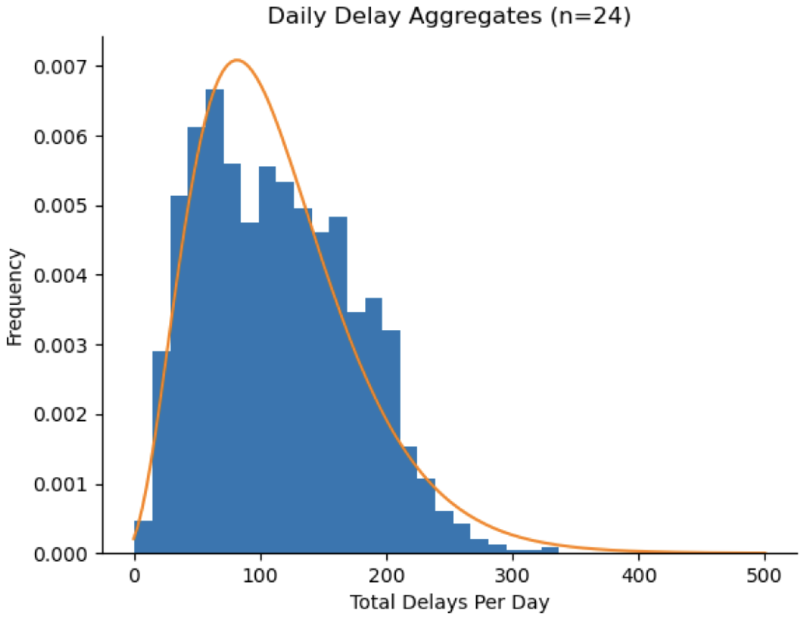
Figure 1 plots the empirical distribution of total daily delay events (n = 24) and the maximum-likelihood Gamma density that best fits these data. The histogram shows a right-skewed pattern. Most days experience roughly 50 to 170 delays, while relatively few days have over 250 delays. The fitted three-parameter Gamma distribution (shape = 3.92, scale = 32.03, location = −11.6) highlights that days with extreme aggregate delay counts, though infrequent, are still plausible. The close alignment between the curve and the histogram supports the fact that a gamma distribution is appropriate. On any given day, it is expected that there will be few delays, as delays generally occur due to rare instances such as mechanical breakdown, weather, or construction. These rare instances do occur, however, as highlighted by the tail of the graph.

Figure 1. Histogram of daily delay aggregates. The histogram was created using a bin size of 24, as calculated by Rice’s Rule. The distribution of total delays per day approximates a gamma distribution, which results in a right-skewed distribution. The maximum number of delays on a given day is 337, while the minimum is 1 delay.

To isolate the incremental value of each covariate class, every model architecture is trained on all eight possible combinations of the three groups (with or without day-of-week, with or without season, with or without weather). Because models respond differently to preprocessing, each covariate blend is presented in up to four data representations: raw numeric form, scaled (scikit-learn’s StandardScaler() function), one-hot-encoded categories, and a scaled + one-hot version. For any given blend, the representation that yields the lowest test RMSE is maintained, ensuring that an ill-suited encoding does not hinder a model.

The earliest 80% (chronologically) of data is used for training, and the remaining 20% of data is used for testing. Prior to the primary bootstrap-based evaluation, model hyperparameter tuning is conducted: 87.5% of the train dataset (70% of the full dataset) is selected as an inner dataset, and the remaining 12.5% of the train dataset (10% of the full dataset) is selected as the validation dataset. Then, for manually selected ranges on model hyperparameters (as specified in this section of our GitHub repository, https://github.com/icoder178/mbta-prediction-models/blob/main/HYPERPARAMETER_TUNING_RANGES.md (accessed on 21 April 2026)), 100 randomized searches are run for each potential combination of task (delay or GSE prediction), feature combination (e.g., including weather but not day of week), and each model (e.g., Random Forest Regression). Since Linear Regression and Moving Average do not need to be tuned, this amounts to $8·2·27·100=\begin{array}{|c|}\hline \mathrm{43,200}\\ \hline\end{array}$ total tuning runs. This is shown in Figure 2.

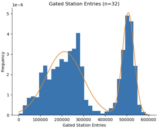
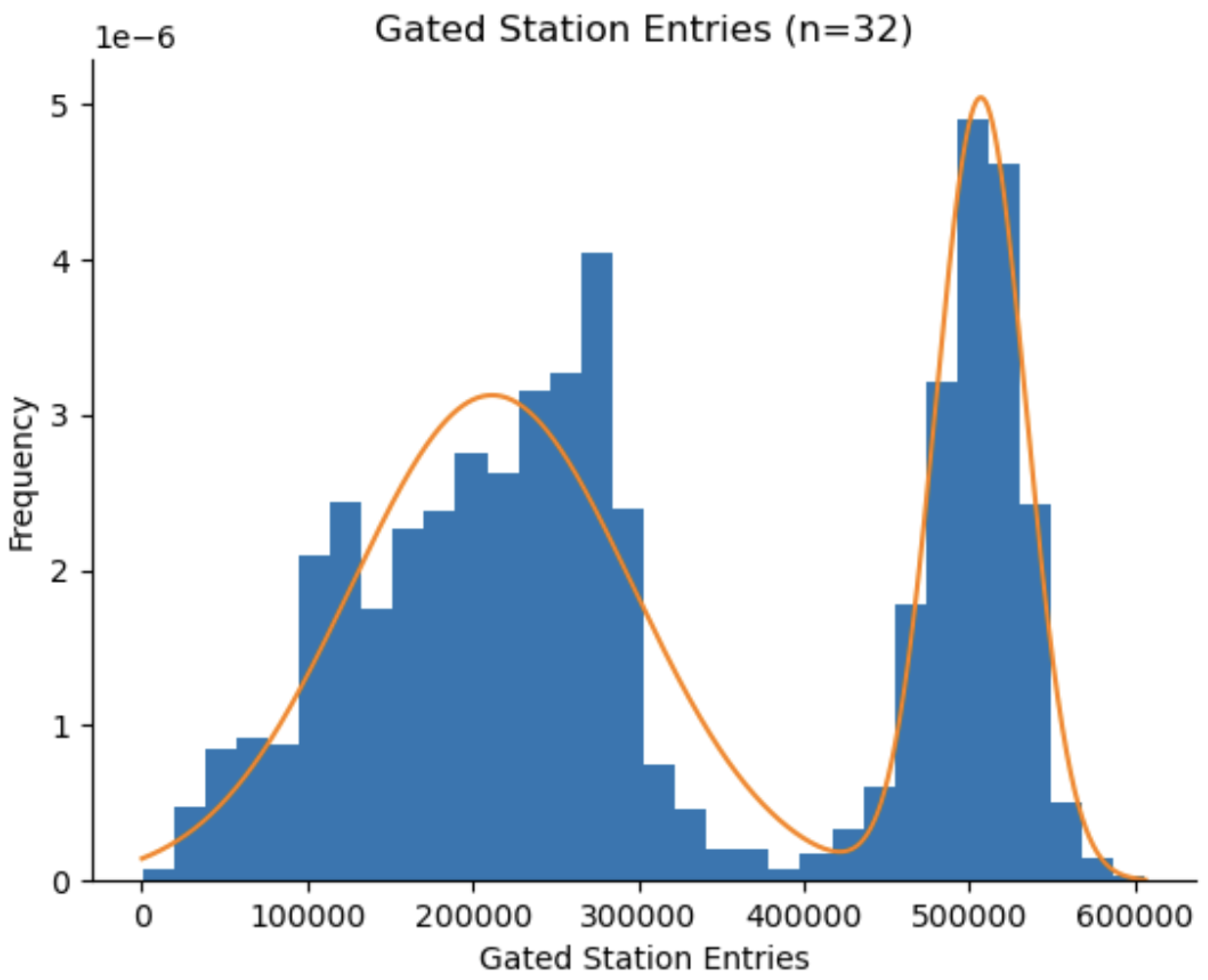
Figure 2. Histogram of gated station entries. The histogram was created using a bin size of 32, calculated according to Rice’s Rule. The distribution of Gated Station Entries follows a bimodal distribution, characterized by two distinct normally distributed peaks. The maximum number of gated station entries on a given day is 606,176, while the minimum was 342. The best-fit curve over the histogram indicates that, on weekdays, more people use the MBTA (e.g., to commute to work/school), as indicated by the first peak at 200,000–300,000 entries. The other peak at 500,000 gated station entries could be due to increased travel on holidays such as Thanksgiving, Christmas, and Independence Day.

Model evaluation then follows a bootstrap protocol [21]. For each model, on each task, for each feature combination, 100 cycles are run. Each cycle creates a bootstrapped train dataset by sampling with replacement from the original train dataset until the bootstrapped dataset is of equivalent size; a bootstrapped test dataset is created in the same manner. Ten architectures are examined: Random Forest, Gradient Boosting, Linear, Ridge, Lasso, Poisson, Support Vector Regression, multilayer perceptron, k-Nearest Neighbor, and a simple moving-average baseline, yielding twenty-seven feature-blend experiments per model per cycle. Two headline statistics are recorded for each architecture: “No Additional Data” RMSE, obtained when the model sees only the lagged target metric, and “Best Added-Feature Set” RMSE, the lowest error achieved across all ways of including additional features (weather, day of week, season) into the dataset. The distribution of these two statistics across the 100 bootstrap replicates yields 95% confidence intervals, allowing us to assess both the raw skill of each model and the extent to which additional covariates enhance its predictive accuracy. Finally, the feature importance of the RandomForest model was then computed through Python’s 3.18SHAP library [22]. Violin plots of the most significant 10 features and SHAP values are in Results.

This grid of covariate permutations, data encodings, and bootstrap resampling makes the comparison robust to sampling variability and preprocessing choices, while highlighting which modeling techniques and input signals most effectively predict next-day MBTA ridership and delay totals.

2.3. Point Process Models

Temporal Point Process Models are used to depict discrete events that occur over time [23]. Time is a continuous variable. In this case, delayed events over time are modeled, and a Hawkes Process run over those.

A Hawkes Process focuses on the “history-dependent” aspect of a point process [24]. In other words, past events can influence the likelihood that another type of event will occur again. This is especially useful for the current problem; for example, when the subway gets delayed, it can lead to additional delays, as tracks must handle more traffic than usual. In the present work, a self-exciting Hawkes Point Process Model is implemented.

Each delay is treated as an event in continuous time and summarizes the past by the history up to time t, ${\mathcal{H}}_t=\{T_i:T_i<t\}$. The (conditional) intensity

$$\lambda (t\mid {\mathcal{H}}_t)=\underset{\Delta t\downarrow 0}{\lim }{\displaystyle \frac{Pr\{\mathrm{an}\mathrm{event}\mathrm{occurs}\mathrm{in}[t,t+\Delta t)\mid {\mathcal{H}}_t\}}{\Delta t}}$$

(1)

is the instantaneous rate at which a new delay is expected to occur, given what has already happened [24]. To capture the tendency of delays to arrive in large quantities, a self–exciting Hawkes Process is used, in which each event temporarily increases the near–future hazard of subsequent events. With an exponential triggering kernel, the above Equation (1) can be re-written as:

$$\lambda (t\mid {\mathcal{H}}_t)=\mu +\sum _{T_i<t}\alpha e^{-\beta (t-T_i)}\{t>T_i\},$$

(2)

where $\mu >0$ is the baseline or background rate, $\alpha >0$ is the immediate jump after an event, and $\beta >0$ controls how quickly that extra risk decays [25]. Two helpful summaries of Equation (2) are the branching ratio $n=\alpha /\beta$, which is the expected number of directly triggered events by a single event, and the half-life $t_{1/2}=\ln 2/\beta$, which is the time for the post-event boost to halve.

Parameters $\mu ,\alpha ,\beta$ are estimated by maximum likelihood from the event times $\left\{T_i\right\}$, using

$$\ell =\sum _i\log \lambda \left(T_i\right)-{\int }_0^T\lambda \left(s\right)ds.$$

(3)

For the exponential kernel, both the compensator $\int \lambda$ and the event-time intensities can be computed in $O\left(N\right)$ via a simple recursion, so fitting scales well to long histories. In practice, history is truncated beyond a few half-lives when evaluating $\lambda \left(t\right)$, which greatly increases computation efficiency with negligible loss of accuracy. Additionally, approximating parameters using Equation (3) is necessary to evaluate the model’s performance.

Two targets are evaluated. For next–event timing, the waiting time from “now” to the next delay is forecasted by Monte Carlo simulation [21] from the fitted intensity (Ogata thinning) and score errors in hours. For daily aggregates, the fitted intensity over each calendar day is integrated, ${\widehat{y}}_d={\int }_d^{d+1}\lambda \left(s\right)ds$, and compared to observed daily totals using RMSE (counts per day). Model performance is checked via cumulative calibration ($N\left(t\right)$ versus $\Lambda \left(t\right)={\int }_0^t\lambda$) and time–rescaling diagnostics.

3. Results and Discussion

3.1. Model Performance (Excluding Hawkes Model)

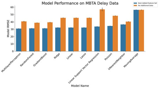
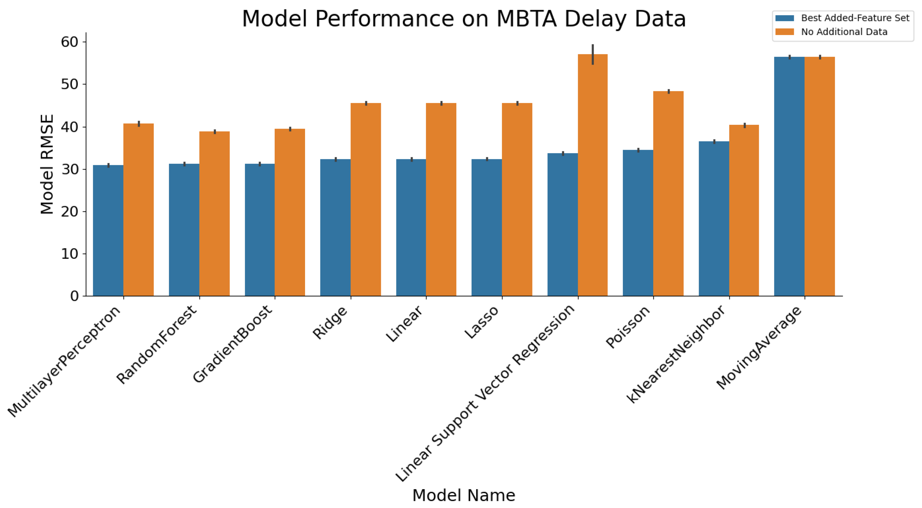
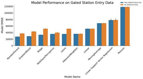
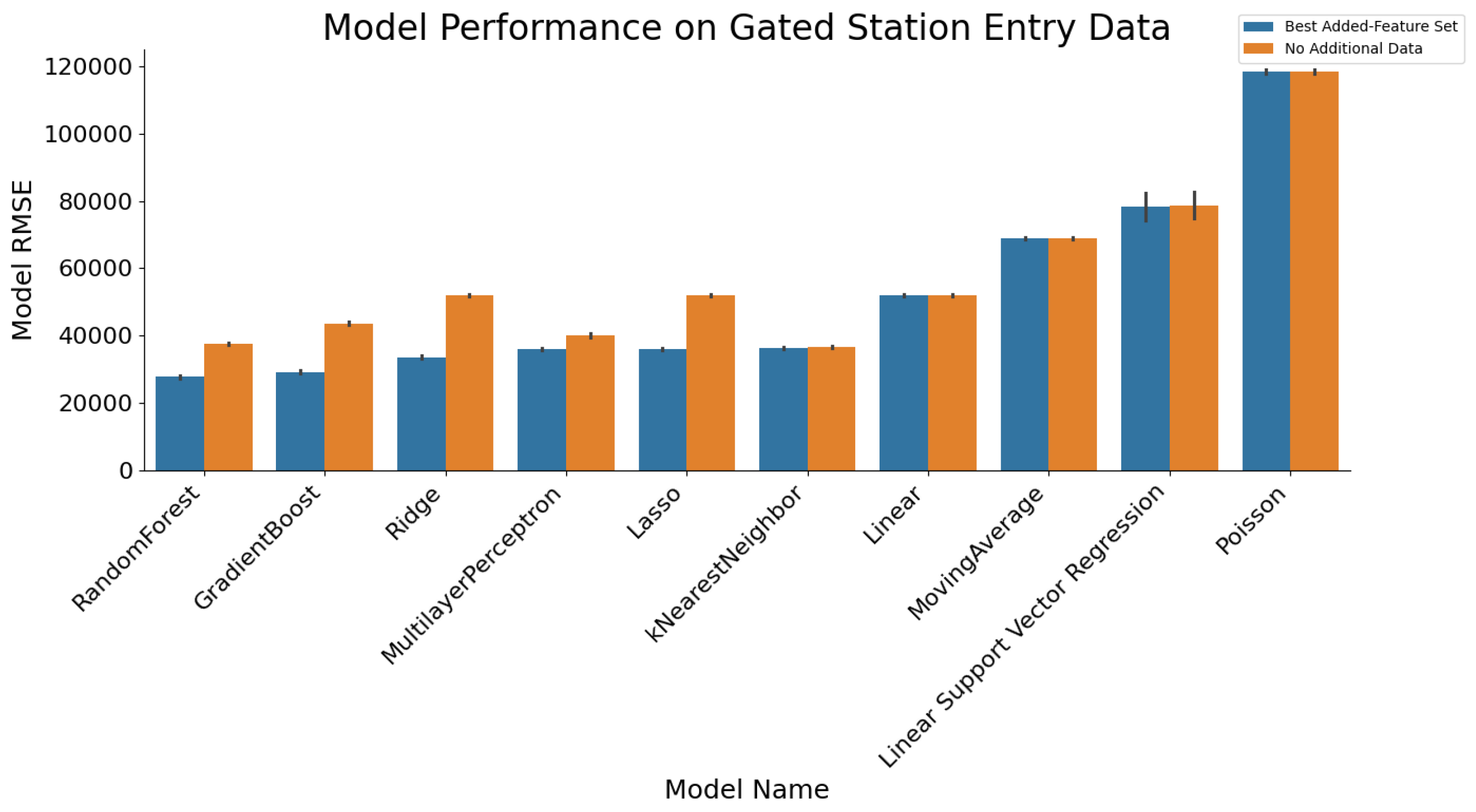
Noticeably, both Figure 3 and Figure 4 highlight that the same three models (Random Forest Regression, Gradient Boost Regression, Multilayer Perceptron) perform well consistently for delay prediction and gated station entry prediction. These suggest that more complex models are better suited to modeling such real-life events compared to simpler models like linear regression. However, ridge regression (aka L2 regression) also performs well, suggesting that even linear regression may be suitable if prevented from overfitting.

Figure 3. Bar graph of model performance on delay data. The bar graph shows that 9 out of 10 models predicted significantly more accurately given additional data, including all three highest-performing models. Additionally, the bar graph indicates that random forest regression, multilayer perceptrons, and gradient boosting regression are most suitable for delay prediction, ranking highest among all models.

Figure 4. Bar graph of model performance on GSE. The bar graph shows 5 of 10 models predicted significantly more accurately given additional data—including all four highest-performing models.

Additionally, the performance of high-performing models on Best Added-Feature Set remains consistently lower than No Additional Data in Figure 3 and Figure 4. This strongly suggests that additional data improves predictive performance, provided model architectures are suited to capturing it.

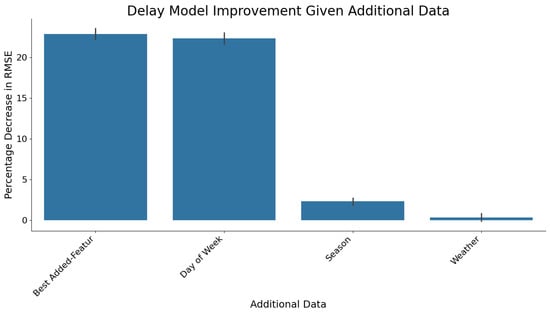
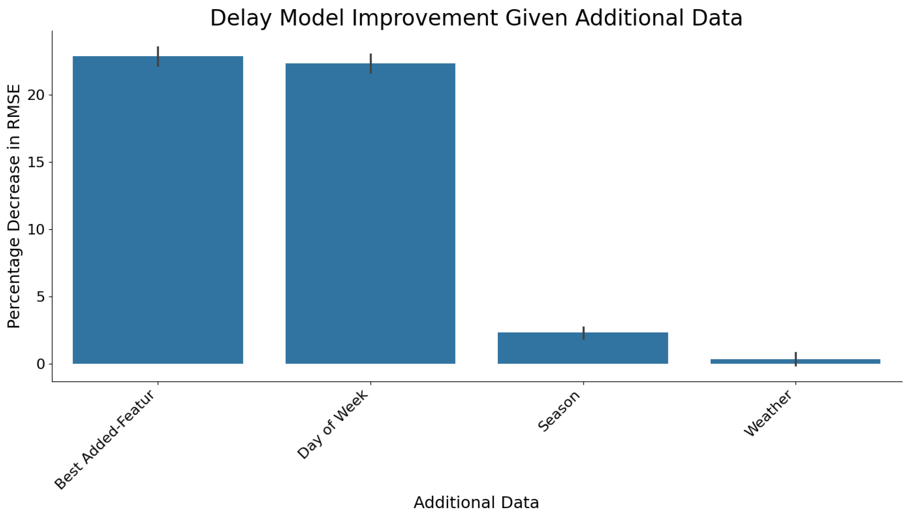
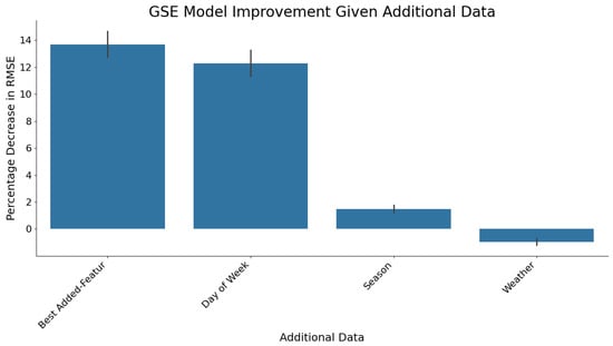
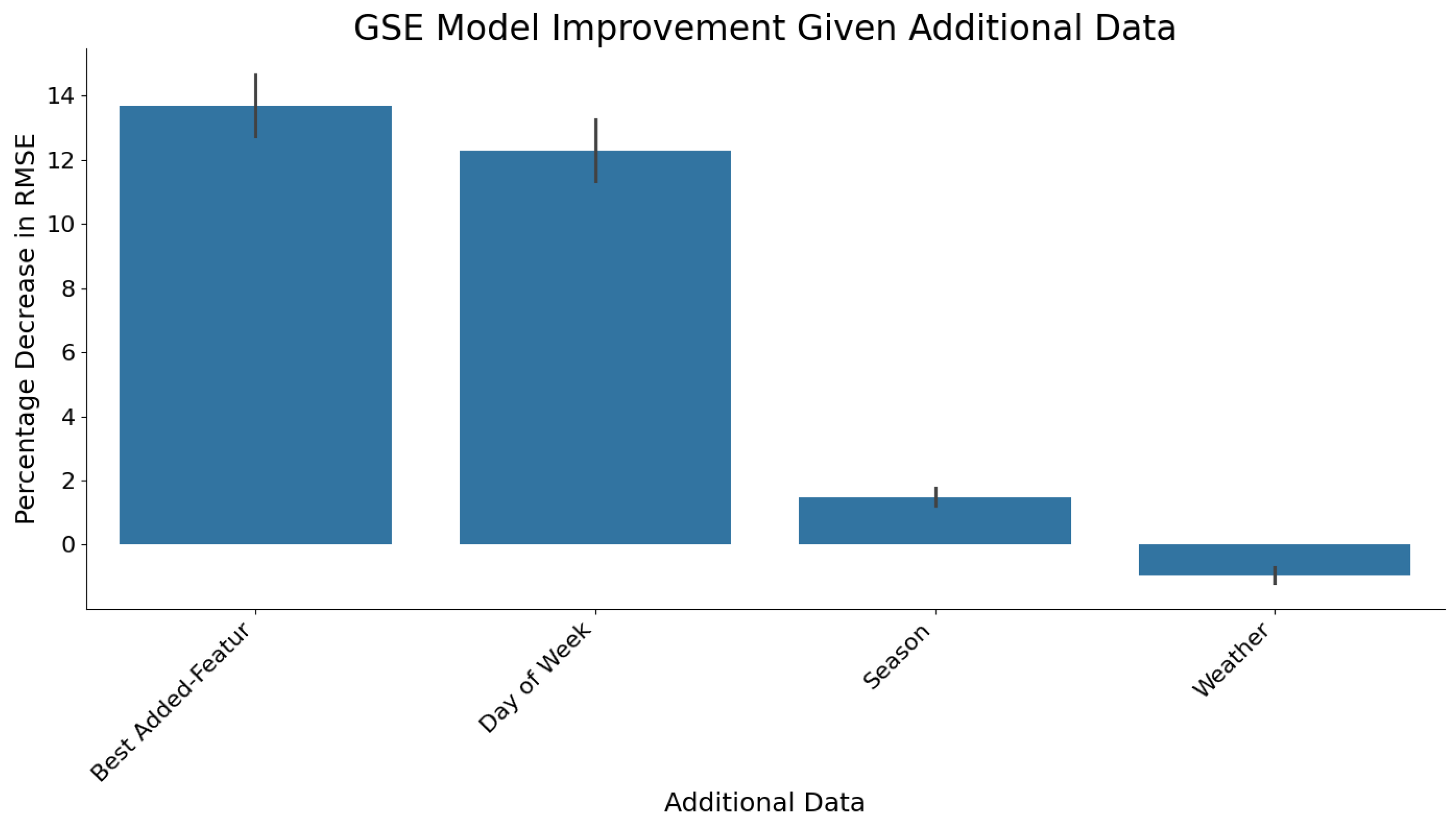
As seen in Figure 5 and Figure 6, providing additional data (day of week, season, weather metrics) leads to tangible improvements in predictive accuracy, especially for high-performance models. This demonstrates some relationship between these metrics and both MBTA delays and train usage; additional data provides useful information.

Figure 5. Bar graph of delay model improvement given additional data. Out of all types of data, the figure shows that day of week data leads to the greatest decrease in error within delay prediction models, while weather data creates almost no decrease in error.

Figure 6. Bar graph of GSE model improvement given additional data. The figure shows that, among the different types of data, day of the week leads to the greatest decrease in error in gated station entry models, while weather leads to the greatest increase in error.

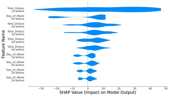
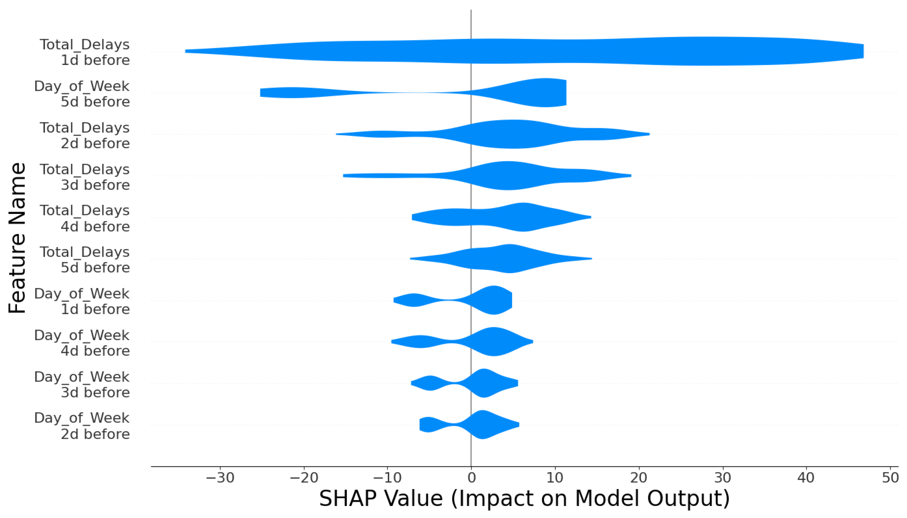
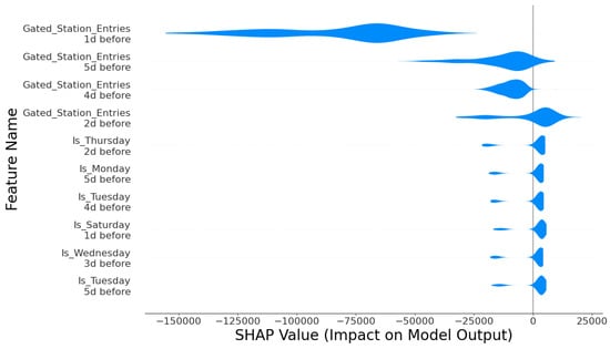
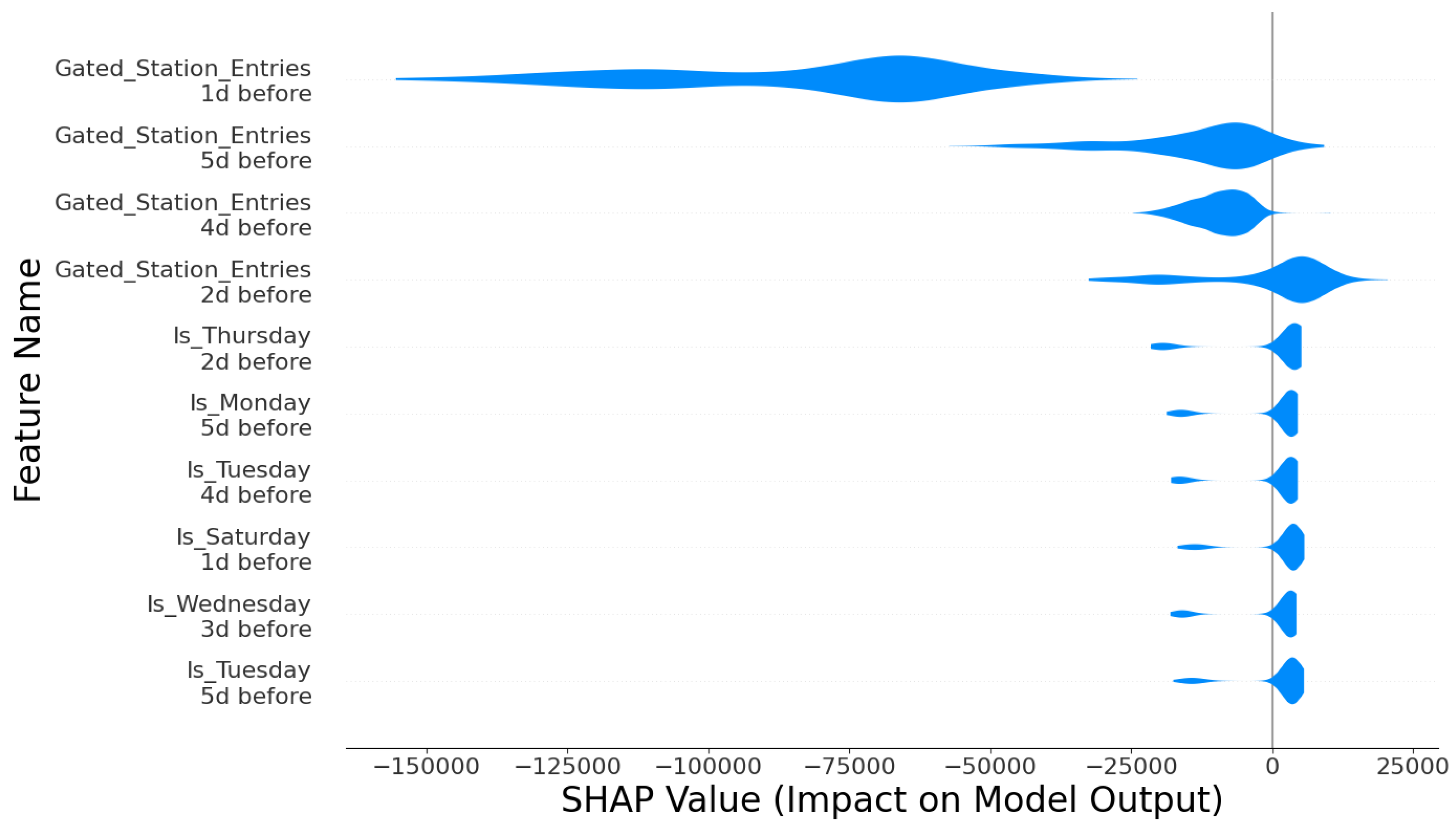
Figure 5 and Figure 6 indicate that including day of week data leads to the greatest improvement in model performance. This is mirrored by the findings in Figure 7 and Figure 8, which show that day of week data is the most important non-target metric factor in model predictions. Thus, this suggests that both delay counts and gated station entries exhibit significant repeating weekly trends that models can leverage to improve performance.

Figure 7. SHAP feature importance values for delay prediction. The graph highlights that the most important factor for delay prediction is total delays in the previous day, followed by the day of week information.

Figure 8. SHAP feature importance values For gated station entry prediction. The graph highlights that the most important factor for gated station entry prediction is gated station entries on the previous few days, followed by day of week information.

3.2. Hawkes Point Process Model Performance

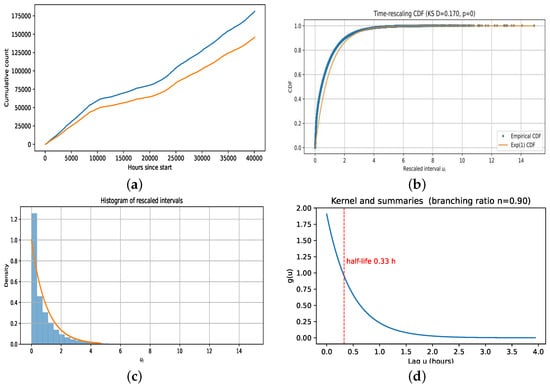
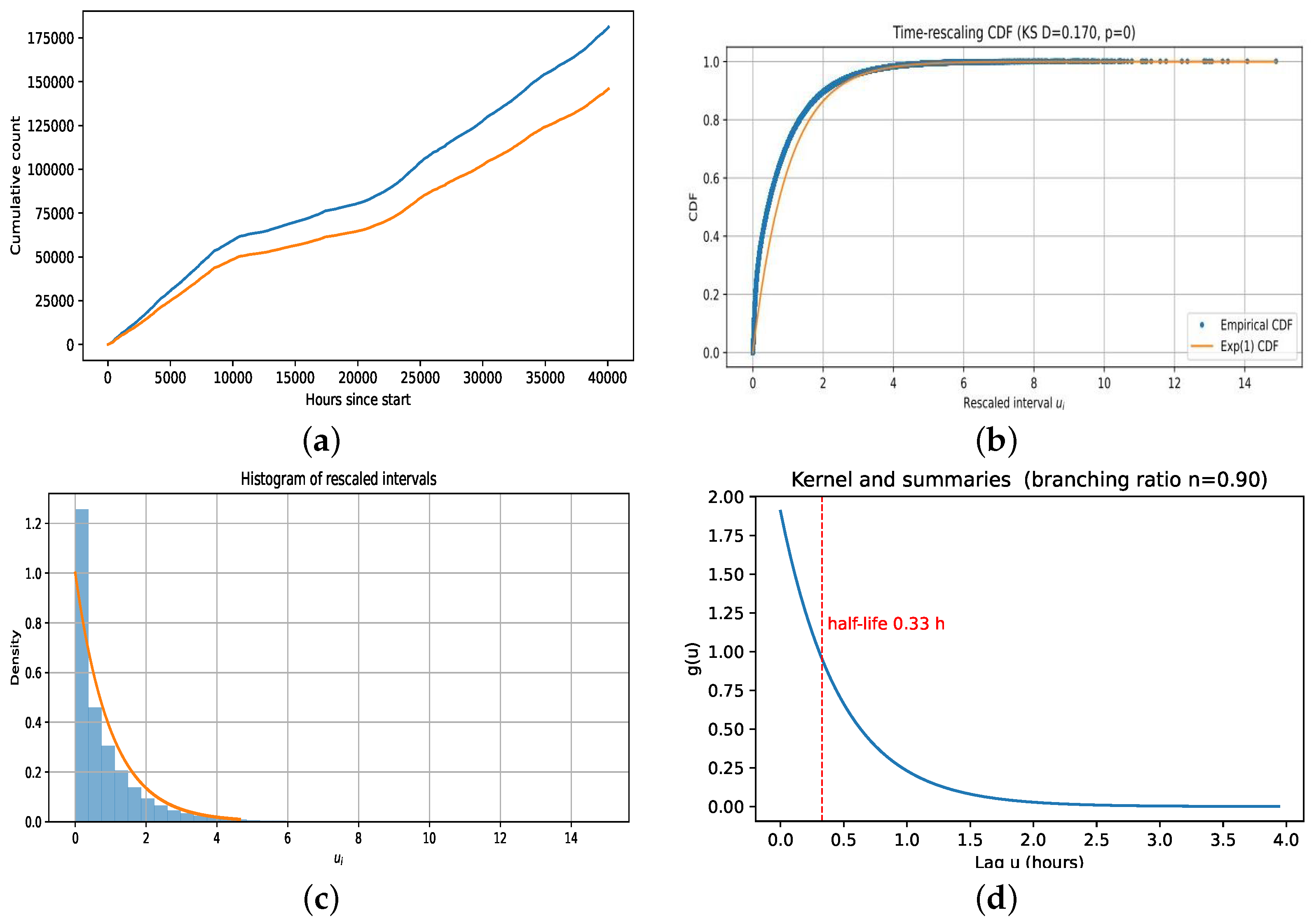
A self–exciting Hawkes Process is fit to the sequence of MBTA delay times, using an exponential triggering kernel $g\left(u\right)=\alpha e^{-\beta u}$ and a constant baseline rate $\mu$. The maximum–likelihood fit yields $\widehat{\mu }=0.438$ events/hour, $\widehat{\alpha }=1.884$, and $\widehat{\beta }=2.087$ (Table 1). Interpreting these numbers, the implied branching ratio is $n=\widehat{\alpha }/\widehat{\beta }=0.90$, so roughly 90% of events are explained as knock–ons from previous events rather than from the baseline. The kernel’s half–life is ${\tau }_{1/2}=\ln 2/\widehat{\beta }=0.33$ hours, meaning the extra risk caused by a delay falls by half in about twenty minutes.

Table 1. Hawkes fit, branching ratio, half-life, and predictive errors.

$\widehat{\mu }$	$\widehat{\alpha }$	$\widehat{\beta }$	$n=\widehat{\alpha }/\widehat{\beta }$	${\tau }_{1/2}=\ln 2/\widehat{\beta }$	Daily RMSE	Next-event RMSE
0.438	1.884	2.087	0.90	0.33 h	137.43 counts	0.670 h

Figure 9a compares the observed cumulative count $N\left(t\right)$ with the model’s expected cumulative intensity $\Lambda \left(t\right)={\int }_0^t\lambda \left(s\right)ds$. The two curves stay close over long periods, but $N\left(t\right)$ tends to edge above $\Lambda \left(t\right)$ during busy spells, suggesting the model is a bit conservative when bursts cascade.

Figure 9. Hawkes diagnostics and learned dynamics. Panels (a–c) assess calibration via cumulative intensity and time-rescaling. Panel (d) summarizes self-excitation strength and decay. (a) Observed $N\left(t\right)$ vs. expected $\Lambda \left(t\right)$. (b) Time-rescaling CDF (ECDF vs. $\mathrm{Exp}\left(1\right)$). (c) Histogram of rescaled intervals $u_i$. (d) Learned kernel $g\left(u\right)=\widehat{\alpha }{e}^{-\widehat{\beta }u}$; half-life and $\mathrm{Exp}\left(1\right)$ pdf and branching ratio annotated.

In Figure 9b, time–rescaling is checked. If the model is well specified, the rescaled inter–event gaps $u_i$ should look like i.i.d. $\mathrm{Exp}\left(1\right)$. The empirical CDF rises slightly faster than the $\mathrm{Exp}\left(1\right)$ benchmark, and the Kolmogorov–Smirnov test [26] reports $D=0.170$ with $p\approx 0$, so the fit is not perfect. The histogram in Figure 9c shows extra mass near zero, consistent with clusters that are tighter than a simple exponential kernel allows.

Figure 9d plots the learned kernel $g\left(u\right)=\widehat{\alpha }{e}^{-\widehat{\beta }u}$. With $n\approx 0.90$, the process is subcritical (hence stable) yet strongly self–exciting: most delays are follow–ons rather than baseline events. The short half–life (about 20 min) indicates that a delay materially raises the chance of another delay within the next hour, and that this effect fades quickly.

Two prediction tasks are evaluated. For daily aggregates, the fitted intensity for each day is integrated to forecast next–day counts; for next–event delay prediction, samples are drawn from the conditional intensity (Ogata thinning) to predict the waiting time to the next delay. On our data, the Hawkes model achieves an RMSE of $137.43$ counts/day for the daily task and $0.670$ hours (40.2 min) for the next–event task (Table 1). Because units differ, daily RMSE is compared to count–forecasting baselines, and next–event RMSE is compared to time–to–event baselines (e.g., empirical inter–arrival summaries). In our study, the Hawkes model trails a tuned moving–average method on daily counts, but it provides calibrated, history–aware next-event predictions and interpretable parameters that quantify how quickly disruptions trigger follow–up delays.

4. Conclusions and Future Research

Despite extensive operational planning, the MBTA system continues to experience both delays and ridership surges, which negatively impact passenger satisfaction. Accurate, data-driven forecasting of these patterns is therefore essential not only for efficient resource allocation but also for informing riders about service reliability. Thus, this work benchmarks multiple statistical and machine learning methods for performance comparison. Our analysis demonstrates that simple calendar features, such as day of the week and seasonality, provide the strongest signals for both daily ridership and delay counts on the MBTA network. Across ten different modeling approaches, the models that incorporated day-of-week flags and seasonal indicators consistently outperformed versions relying solely on weather variables. In fact, adding weather data by itself sometimes slightly degraded performance, confirming that passenger flows and delay patterns are driven more by human schedules than by meteorological factors.

Among the machine-learning techniques benchmarked, ensemble methods and multilayer perceptrons achieved the lowest RMSEs. Random Forest and Gradient Boosting models, in particular, were the most robust and are promising candidates for day-ahead forecasting of MBTA outcomes. Complementing these aggregate predictors, a self-exciting Hawkes Point Process is fitted to the delay event times. The fitted model revealed strong but short-lived self-excitation (branching ratio ≈ 0.9; half-life ≈ 0.33 h), meaning that one delay noticeably increases the chance of another within the next hour, and then the effect fades quickly. While the Hawkes model underperformed simple moving-average baselines on day-level count prediction, it provided promising next-event prediction with interpretable results, and its diagnostic plots (cumulative calibration and time-rescaling) highlighted when bursts were under- or over-estimated. Practically, this suggests a significant distinction: calendar-driven ML models remain best suited for day-ahead volumes, while the Hawkes model is most useful for real-time dispatch and crowd reduction, where quantifying short-term clustering of disruptions is crucial.

It is worth noting that simpler time-series models (e.g., ARIMA [27]) were not used in this research. This was primarily due to the poor performance of the Hawkes model (RMSE >130 counts/day, compared to RMSE <60 for a simple moving average), as observed when handling daily aggregates. This was likely because, given the number of events each day, any statistical model tends to regress to its mean due to the law of large numbers. Other time series models would encounter similar issues, making an investigation into using them for handling daily aggregates not worthwhile.

Looking ahead, several directions remain plausible to extend our work. Our current analysis aggregates most inputs at the daily level; moving to hourly or station-level resolution could uncover localized effects and strengthen both the ML and point-process components. Incorporating operational variables—such as train assignments, crew shifts, maintenance windows, unplanned incidents, and major events—should help explain residual variation and improve forecast accuracy. Finally, embedding spatial network structure (e.g., line topology and transfer hubs) into both the predictive models and the Hawkes kernel could capture how disruptions propagate through the system. With these enhancements, future models can deliver more precise guidance to transit agencies and their riders, combining reliable day-ahead planning with actionable, real-time risk estimates of cascading delays.

In short, our key conclusions are that models like Random Forest and Gradient Boost appear most effective at predicting daily aggregates under real-world conditions, and that fitting a Hawkes Point Process suggests that the chance of delay increases immediately following a prior delay.

Future research extensions include handling higher-resolution data and incorporating additional variables to improve predictive accuracy.

References

- Singhal, A.; Kamga, C.; Yazici, M.A. Impact of Weather on Urban Transit Ridership. Transp. Res. Part A Policy Pract. 2014, 69, 379–391. [Google Scholar] [CrossRef] [Scilit]
- Guo, Z.; Wilson, N.; Rahbee, A. Impact of Weather on Transit Ridership in Chicago, Illinois. Transp. Res. Rec. 2007, 2034, 3–10. [Google Scholar] [CrossRef] [Scilit]
- Saneinejad, S.; Roorda, M.J.; Kennedy, C. Modeling the impact of weather conditions on active transportation travel behavior. Transp. Res. Part D Transp. Environ. 2012, 17, 129–137. [Google Scholar] [CrossRef] [Scilit]
- Wei, M.; Corcoran, J.; Sigler, T.; Liu, Y. Modeling the Influence of Weather on Transit Ridership: A Case Study from Brisbane, Australia. Transp. Res. Rec. 2018, 2672, 505–510. [Google Scholar] [CrossRef] [Scilit]
- Massachusetts Bay Transportation Authority (MBTA). Ridership—The T Performance Metrics. 2025. Available online: https://www.mbta.com/performance-metrics/ridership-the-t (accessed on 5 August 2025).
- Citizens Transit. The Five Largest U.S. Public Transit Systems. Available online: https://citizenstransit.org/node/67 (accessed on 5 August 2025).
- MassINC Polling Group. Residents Sound the Alarm on MBTA Service Quality & Safety. 2025. Available online: https://www.massincpolling.com/our-work/poll-residents-sound-the-alarm-on-mbta-service-quality-safety (accessed on 5 August 2025).
- Zhang, Q.; Ma, Z.; Zhang, P.; Ling, Y.; Jenelius, E. Real-Time Bus Arrival Delays Analysis Using Seemingly Unrelated Regression Model. Transportation 2024, 53, 571–602. [Google Scholar] [CrossRef] [Scilit]
- Gohil, B.N.; Tzionas, P.; Ramyaa, K.; Chatterjee, S. Rail Transit Delay Forecasting with Causal Machine Learning. In Proceedings of the Proceedings of the 1st ACM SIGSPATIAL International Workshop on Spatiotemporal Causal Analysis (STCausal ’24); ACM: New York, NY, USA, 2024; pp. 15–24. [Google Scholar] [CrossRef] [Scilit]
- Wang, J.; Shalaby, A. DST-TransitNet: A Dynamic Spatio-Temporal Deep Learning Model for Scalable and Efficient Network-Wide Prediction of Station-Level Transit Ridership. arXiv 2024, arXiv:2410.15013. [Google Scholar]
- He, Y.; Li, L.; Zhu, X.; Tsui, K.L. Multi-Graph Convolutional-Recurrent Neural Network (MGC-RNN) for Short-Term Forecasting of Transit Passenger Flow. arXiv 2021, arXiv:2107.13226. [Google Scholar]
- Tiong, K.Y.; Corman, F.; Lodewijks, G. A Review of Data-Driven Approaches to Predict Train Delays. Transp. Res. Part C Emerg. Technol. 2023, 147, 104027. [Google Scholar] [CrossRef] [Scilit]
- Barbour, W.; Martinez Mori, J.C.; Kuppa, S.; Work, D.B. Prediction of Arrival Times of Freight Traffic on US Railroads Using Support Vector Regression. Transp. Res. Part C Emerg. Technol. 2018, 93, 211–227. [Google Scholar] [CrossRef] [Scilit]
- Marković, N.; Milinković, S.; Tikhonov, K.S.; Schonfeld, P. Analyzing Passenger Train Arrival Delays with Support Vector Regression. Transp. Res. Part C Emerg. Technol. 2015, 56, 251–262. [Google Scholar] [CrossRef] [Scilit]
- Bapaume, T.; Côme, E.; Ameli, M.; Roos, J.; Oukhellou, L. Forecasting Passenger Flows and Headway at Train Level for a Public Transport Line: Focus on Atypical Situations. Transp. Res. Part C Emerg. Technol. 2023, 153, 104195. [Google Scholar] [CrossRef] [Scilit]
- Ruiz, E.; Yushimito, W.F.; Aburto, L.; de la Cruz, R. Predicting Passenger Satisfaction in Public Transportation Using Machine Learning Models. Transp. Res. Part A Policy Pract. 2024, 181, 103995. [Google Scholar] [CrossRef] [Scilit]
- Meteostat. Station 72509: Daily Weather Observations, 2018-12-31. 2025. Available online: https://meteostat.net/en/station/72509?t=2025-08-06/2025-08-06 (accessed on 1 July 2025).
- Massachusetts Bay Transportation Authority (MBTA). MBTA Service Alerts—ArcGIS Open Data Dataset. 2025. Available online: https://mbta-massdot.opendata.arcgis.com/datasets/mbta-service-alerts/explore (accessed on 1 July 2025).
- Bishop, C. Pattern Recognition and Machine Learning; Springer: Berlin/Heidelberg, Germany, 2016. [Google Scholar]
- Hastle, T. Elements of Statistical Learning; Pearson: London, UK, 2018. [Google Scholar]
- ScienceDirect Topics. Bootstrapping. Available online: https://www.sciencedirect.com/topics/earth-and-planetary-sciences/bootstrapping (accessed on 27 November 2025).
- SHAP Developers. SHAP Documentation. Available online: https://shap.readthedocs.io/en/latest/ (accessed on 27 November 2025).
- Zhang, X.; Aravamudan, A. A Generalized Time Rescaling Theorem for Temporal Point Processes. Neural Comput. 2025, 37, 871–885. [Google Scholar] [CrossRef] [Scilit] [PubMed]
- Bernabeu, A.; Zhuang, J.; Mateu, J. Spatio-Temporal Hawkes Point Processes: A Review. J. Agric. Biol. Environ. Stat. 2025, 30, 89–119. [Google Scholar] [CrossRef] [Scilit]
- Jones-Todd, C.M.; van Helsdingen, A.B.M. The R Package Stelfi—Univariate Hawkes Process. Available online: https://cmjt.github.io/stelfi/univariate-hawkes.html (accessed on 27 November 2025).
- NIST/SEMATECH e-Handbook of Statistical Methods. Kolmogorov–Smirnov Goodness-of-Fit Test (Section 1.3.5.16). 2003. Available online: https://www.itl.nist.gov/div898/handbook/eda/section3/eda35g.htm (accessed on 28 November 2025).
- Noble, J. What Are ARIMA Models? 2025. Available online: https://www.ibm.com/think/topics/arima-model (accessed on 28 November 2025).
Disclaimer/Publisher’s Note: The statements, opinions and data contained in all publications are solely those of the individual author(s) and contributor(s) and not of MDPI and/or the editor(s). MDPI and/or the editor(s) disclaim responsibility for any injury to people or property resulting from any ideas, methods, instructions or products referred to in the content. |
© 2026 by the authors. Licensee MDPI, Basel, Switzerland. This article is an open access article distributed under the terms and conditions of the Creative Commons Attribution (CC BY) license.