


Abstract
Characterizing the urban background atmosphere in equatorial regions is challenging due to the complex monsoonal, diurnal, and human dynamics. This study evaluates the atmospheric steady-state of a university campus in Brunei Darussalam by monitoring the canopy layer at high resolution over 6 months. Non-parametric variance testing and random forest regression modeled the Pollutant Standard Index (PSI) alongside meteorological and operational variables. Kruskal–Wallis testing revealed that while PSI remains consistently “Good”, it shows significant sensitivity to diurnal (H = 99.03) and academic operational (H = 15.46) factors, isolating NO2 as a distinct anthropogenic tracer (H = 30.73 across academic terms). Optimizing the random forest regressor with the previous day’s autoregressive lag term enhanced predictive performance (R2 = 0.961, RMSE = 1.46, and MAPE = 10.42%). Feature importance analysis demonstrates that atmospheric persistence governs the baseline physics, whereas air temperature and relative humidity regulate immediate contemporary variations. This predictive framework provides a robust environmental management benchmark for stable, low-pollution tropical canopy environments.
1. Introduction
The rapid urbanization and industrialization across Southeast Asia have compromised regional air quality, raising public health and environmental sustainability concerns. In regional education settings, nitrogen dioxide (NO2) levels often exceed the World Health Organization (WHO) standards due to construction and student commuting [1]. Equatorial zones maintain clean urban-background profiles but remain susceptible to seasonal transboundary haze from biomass burning and peatland fires [1,2,3]. In these coastal equatorial zones, the atmospheric steady-state is governed by a complex interplay between the tropical diurnal cycle and mesoscale circulations (e.g., sea/land-breeze systems) that influence the dispersion of ground-level ozone (O3) and precursors, including nitrogen oxides (NOx), volatile organic compounds (VOCs), and carbon monoxide (CO) [4,5,6].
Atmospheric vertical profiles are highly dynamic; fine particulate matter (PM2.5) concentrations can decrease by up to 33% at the rooftop level compared to curbside measurements due to atmospheric stability and wind shear [7,8]. Thus, monitoring within the Urban Canopy Layer (UCL) provides a stabilized vantage point where macroscopic meteorological dynamics exert greater influence than localized street-level emissions [9,10,11,12,13]. While 5 min intervals capture transient emission peaks [14], 1 h temporal aggregation captures fine-scale diurnal photochemical cycles more effectively than daily averages [15,16,17], filtering out high-frequency stochastic instrumental noise while aligning with standard public health reporting frameworks [18].
Seasonality in the Maritime Continent is defined by the biannual monsoon system, the primary regulator of particulate distribution. Elevated concentrations of coarse particulate matter (PM10) and PM2.5 are consistently recorded during the Southwest (SW) monsoon and inter-monsoon periods due to dry conditions and transboundary smoke transport [2,19]. Analyzing these complex, non-linear environmental datasets require robust statistical frameworks, as air quality data typically exhibits right-skewed, non-normal distributions with frequent outliers [20,21]. Non-parametric approaches (such as Kruskal–Wallis tests and kernel estimators) have proven effective for comparing populations and forecasting pollution episodes without the constraints of distribution-dependent assumptions [22,23,24,25,26].
To transition from observation to predictive intelligence, machine learning frameworks like random forest regression have emerged as high-capacity tools. Random forest models can achieve R2 scores of 0.86 using meteorological drivers alone, even in remote, low-pollution environments [27,28]. These models achieve high performance in tropical campus settings (R2 ≈ 0.91) [29], whereas accuracy in urban temperate climates is lower (R2 ≈ 0.72 in Seoul, South Korea [30] and R2 ≈ 0.73 in Ankara, Turkey [31]). Incorporating temporal lag variables and meteorological inputs significantly improves model prediction accuracy, providing a precise mechanism for resolving the influence of natural versus human-induced drivers [3,32]. Despite these advancements, there remains a lack of high-resolution vertical monitoring data bridging the gap between localized academic operational cycles and seasonal drivers in Brunei Darussalam.
This study aims to characterize the atmospheric steady-state of an equatorial university campus by evaluating the sensitivity of the UCL to natural and anthropogenic pressures. The specific objectives are to (i) assess the seasonal baseline and diurnal distributions of pollutants and meteorological drivers; (ii) evaluate the statistical sensitivity of the PSI and individual pollutants to the diurnal cycle and academic operational status; and (iii) assess the predictive influence and feature importance of meteorological, temporal, and anthropogenic variables using a random forest regressor. Consequently, this work establishes a high-fidelity air quality benchmark for the region while demonstrating predictive modeling’s capacity to resolve subtle tropical atmospheric drivers.
2. Materials and Methods
2.1. Site Description and Instrumentation
Atmospheric monitoring was conducted at an equatorial university campus in Brunei Darussalam (4.98° N, 114.90° E). To isolate background signal from transient perturbations, a Kunak Air Pro (Kunak Technologies S.L., Orcoyen, Spain) monitoring station was deployed at an elevation of about 16.6 m within the UCL, filtering localized surface noise while retaining sensitivity to vertical dispersion dynamics [7]. The campus setting features administrative-academic infrastructure interspersed with secondary vegetation, establishing a localized profile driven by campus vehicular transit without industrial interference.
Continuous measurements spanned from 26 August 2025 to 25 February 2026, covering three distinct seasonal phases: the end of the SW monsoon (August–September 2025), the Inter-monsoon 2 period (October–November 2025), and the Northeast (NE) monsoon (December 2025–February 2026). This approach maintained an uninterrupted time series across the entire monitoring period. The instrumentation captured ambient concentrations of PM2.5, PM10, O3, and NO2, along with primary meteorological drivers (air temperature, relative humidity, and wind speed). Raw data collected at 5 min intervals were aggregated to 1 h averages. No major localized fire anomalies occurred during the monitoring timeframe, confirming that the recorded measurements reflect the baseline background atmosphere.
2.2. Pollutant Standard Index (PSI) Framework
The air quality status was quantified using the Pollutant Standard Index (PSI), with calculation procedures and breakpoints adopted from Singapore’s National Environment Agency (NEA) [18]. The overall PSI was derived from a multi-pollutant suite including 24 h averages for PM2.5, PM10, and sulfur dioxide (SO2); 8 h averages for O3 and CO; and 1 h averages for NO2. During the monitoring period, SO2 concentrations remained consistently at zero, while CO levels were negligible (<25.6 mg/m3 8 h average), posing no risk to the index calculation. Consequently, these two air pollutants were excluded from the detailed statistical analysis to focus on the more dynamic seasonal drivers.
Following Singapore’s NEA guidelines, air quality was categorized into a five-tier health risk scale: Good (0 < PSI < 50), Moderate (51 < PSI < 100), Unhealthy (101 < PSI < 200), Very Unhealthy (201 < PSI < 300), and Hazardous (PSI > 300). The sub-index (Ip) for each pollutant is calculated using piecewise linear interpolation across predefined breakpoint thresholds according to Equation (1):
where Bhigh and Blow are the upper and lower concentration breakpoints enclosing the observed value Cp, while Ihigh and Ilow are the corresponding sub-index limits. The overall PSI is then determined by the maximum sub-index value calculated across all monitored pollutants, as defined by Equation (2):
2.3. Statistical Analysis and Predictive Modeling
Dataset processing and modeling were conducted using JASP (Version 0.96) via a multi-stage statistical hierarchy to ensure robust characterization.
2.3.1. Descriptive Diagnostics and Distribution Testing
Initial data exploration involved calculating primary descriptive metrics (arithmetic mean, standard deviation, and maximums) for all atmospheric pollutants and meteorological parameters across the three monsoon seasons. The dataset comprises 4409 hourly observations across the SW (n = 863), Inter-monsoon 2 (n = 1462), and NE (n = 2084) monsoons. To assess data normality, the Shapiro–Wilk test was applied, along with a quantitative assessment of skewness. These diagnostics dictated the selection of non-parametric procedures for downstream comparative analysis. Visual distributions were rendered as integrated boxplots and violin plots, split by monsoon seasons, to illustrate the interquartile ranges and kernel density for each parameter.
2.3.2. Non-Parametric Variance Analysis
The Kruskal–Wallis H-test (a rank-based non-parametric alternative to one-way ANOVA) was conducted to evaluate the influence of anthropogenic and natural factors. The H-statistic was evaluated for the PSI and individual pollutants, with academic status (term, break, and holiday) and diurnal cycle (day and night) as fixed factors. Where significant differences were identified (p < 0.05), Dunn’s post hoc tests were performed. To maintain a conservative approach and minimize Type I error risks, both Bonferroni and Holm corrections were applied. Significant results are reported specifically where the adjusted p-value (pHolm) remained below the 0.05 threshold. The magnitude of the non-parametric group differences was quantified using rank epsilon-squared (Rank ε2), where values near 0.01 indicate a small effect, 0.06 a medium effect, and ≥0.14 a large effect size.
2.3.3. Random Forest Regression
Predictive modeling within non-linear, highly correlated environmental time series requires frameworks capable of partitioning high-dimensional feature spaces without assuming distribution normality [33,34]. Accordingly, a random forest regressor was implemented to model the stochastic relationship between environmental drivers and PSI. The model was optimized using an 80/20 train/test split, with an internal 20% validation subset drawn from the training set to prevent overfitting. To resolve temporal autocorrelation, the previous day’s PSI lagged input feature (PSIt−1) was integrated into the modeling matrix alongside contemporaneous meteorological inputs (air temperature, relative humidity, and wind speed) and discrete categorizations (diurnal cycle, day of the week, monsoon season, and academic status).
The model configuration applied an optimized ensemble of 500 trees, with each tree utilizing 50% of the training data. Feature selection per split was set to “Auto” to maximize the decorrelation between individual decision trees. Features were scaled for consistency, and a fixed seed of 123 was applied to ensure the reproducibility of the prediction results. The model was evaluated using the coefficient of determination (R2), root mean square error (RMSE), mean absolute error (MAE), and mean absolute percentage error (MAPE), while feature importance was assessed via mean decrease in accuracy.
3. Results
3.1. Seasonal Characterization and Distribution Dynamics
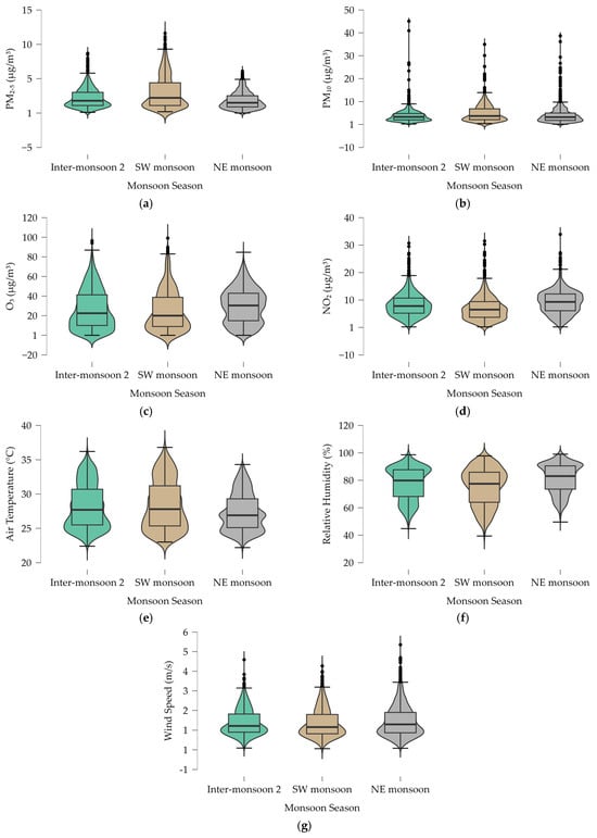
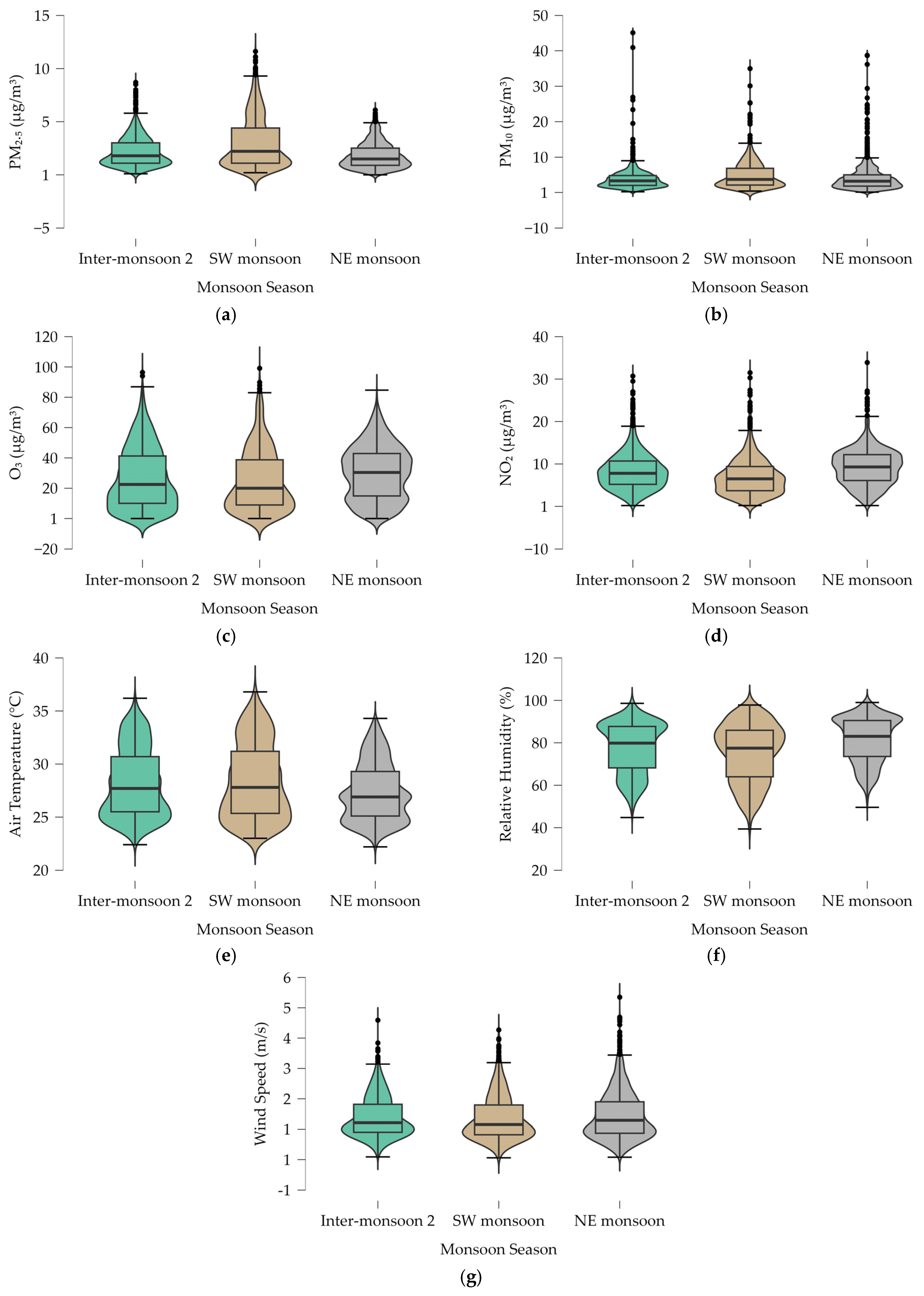
The atmospheric data presented in Table 1 confirm that air quality at the observatory remained within the “Good” range of PSI throughout the monitoring period. However, distinct seasonal shifts are evident, particularly for particulate matter. PM2.5 and PM10 peaked during the SW monsoon, with mean concentrations of 3.01 ± 2.40 µg/m3 and 4.83 ± 3.78 µg/m3, respectively. In contrast, the NE monsoon recorded the lowest PM2.5 level of 1.80 ± 1.18 µg/m3. The distribution features shown in Figure 1a–d reveal high probability density at low concentrations for all pollutants, validating a clean background state at the 16.6 m canopy height. Outliers (black dots in Figure 1) indicate episodic variations from transient plumes or localized stagnation.
Table 1.
Descriptive statistics of atmospheric pollutants and meteorological parameters by monsoon season.
Figure 1.
Distribution of atmospheric pollutants and meteorological parameters across monsoon seasons. (a) PM2.5 concentrations; (b) PM10 concentrations; (c) ground-level O3 concentrations; (d) NO2 concentrations; (e) ambient air temperature; (f) relative humidity; (g) wind speed. Notes: Boxplots represent the median and interquartile range; violin plots illustrate kernel density estimates.
As shown in Table 1, relative humidity exhibited negative skewness across all seasons (e.g., −0.49 during inter-monsoon 2), reflecting a maritime distribution biased toward high saturation, as visualized by the upward-tapering violin plots in Figure 1f. Ambient air temperature (Figure 1e) and O3 concentrations (Figure 1c) followed a rigorous diurnal coupling, with O3 reaching a maximum of 99.1 µg/m3 during the SW monsoon. This peak coincides with the highest recorded temperature of 36.8 °C. The wind speed distribution (Figure 1g) confirms a predominant low-velocity regime (mean < 1.5 m/s).
3.2. Statistical Sensitivity to Operational and Diurnal Cycles
The Kruskal–Wallis H-test (Table 2) reveals a distinct hierarchy of environmental and anthropogenic influences on the atmospheric steady state. The PSI demonstrates high statistical sensitivity to both academic status (H = 15.46, p < 0.001, Rank ε2 = 0.004) and the diurnal cycle (H = 99.03, p < 0.001, Rank ε2 = 0.022). Post hoc comparisons via Dunn’s test for the PSI identified significant differences in the holiday-term and break-holiday pairs.
Table 2.
Non-parametric variance analysis (Kruskal–Wallis) and post hoc comparisons.
Individual pollutant behaviors varied widely. NO2 showed high diurnal sensitivity (H = 598.3, p < 0.001, Rank ε2 = 0.136) and uniquely displayed a significant comparative difference between the break and term periods (H = 30.73, p < 0.001, Rank ε2 = 0.007). Conversely, O3 variance remained entirely independent of academic status (p = 0.318, Rank ε2 < 0.001) and was strictly governed by the diurnal cycle (H = 319.7, p < 0.001, Rank ε2 = 0.073).
3.3. Predictive Influence and Feature Importance
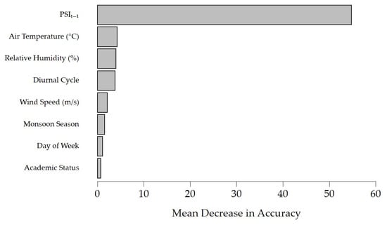
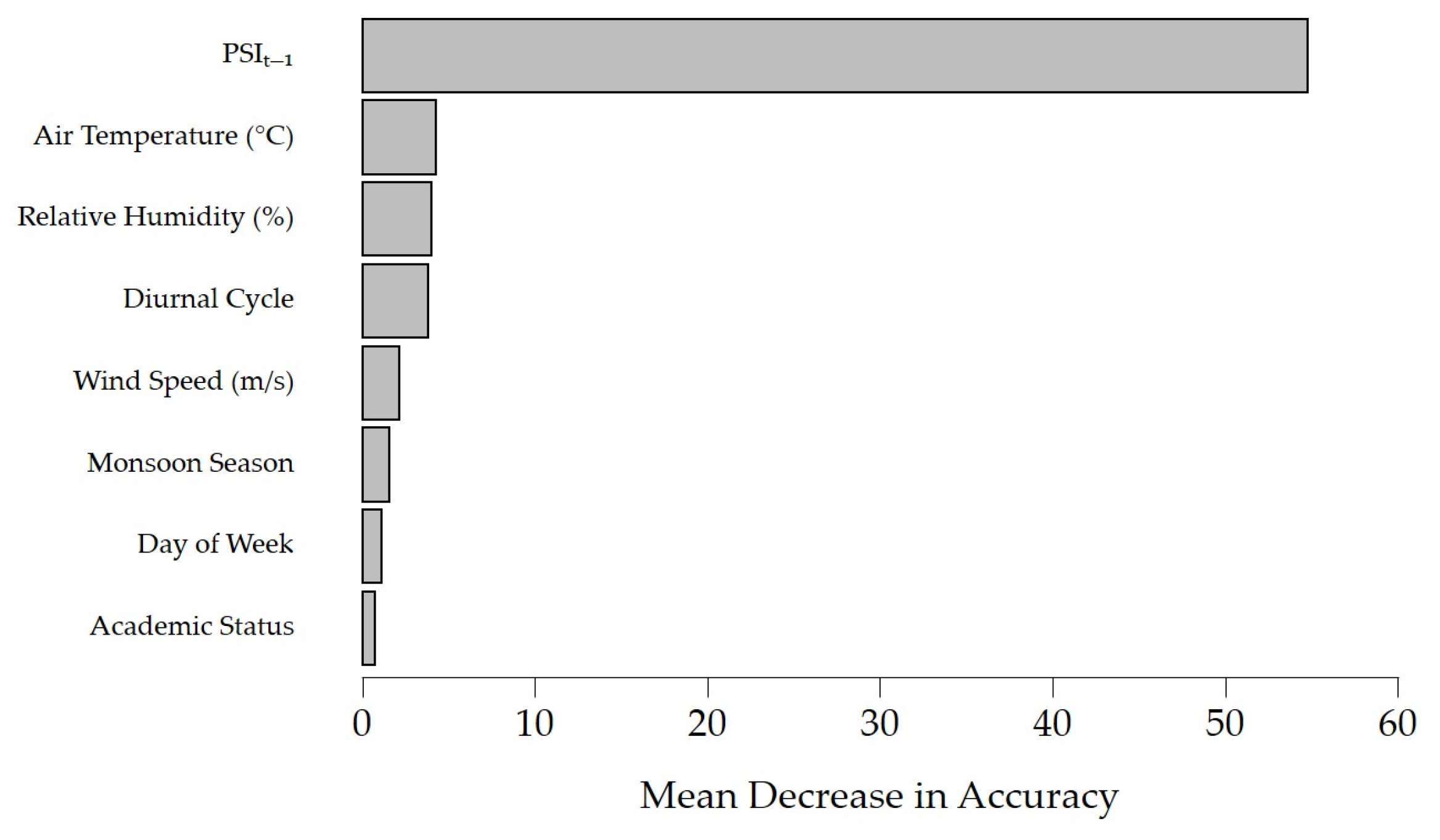
Integration of the autoregressive lag term (PSIt−1) substantially improved the random forest model, yielding an R2 of 0.961, RMSE of 1.46, MAE of 1.13 and MAPE of 10.42% (compared to an R2 of 0.477, RMSE of 4.76, MAE of 3.76 and MAPE of 35.77% for the non-lagged model). Feature importance based on the mean decrease in accuracy metric (Figure 2) identifies PSIt−1 as the dominant predictor (score: 54.76). Among contemporary parameters, air temperature showed the highest relative importance (4.26), followed by relative humidity (4.03), diurnal cycle (3.83), and wind speed (2.15). Macro-scale and operational features exerted negligible predictive influence (monsoon season: 1.57; day of the week: 1.13; academic status: 0.76).
Figure 2.
Random forest feature importance for predicting PSI based on mean decrease in accuracy.
4. Discussion
The low absolute concentrations and baseline stability in Table 1 demonstrate that the campus maintains a clean background state. The seasonal elevation of PM2.5 and PM10 during the SW monsoon reflects the site’s susceptibility to transboundary regional transport, which matches established patterns observed across the Maritime Continent, where dry seasonal monsoonal flows carry aged biomass burning plumes northward [3]. This regional background signal is captured clearly within the UCL.
The microenvironmental elevation of 16.6 m serves as an effective physical filter, isolating the background atmospheric state. By remaining elevated above street level, the observatory smooths out localized curbside fluctuations, explaining the high probability density at very low concentrations observed in the violin plots. The low-velocity wind regime (mean < 1.5 m/s) indicates that localized mechanical dispersion is weak, allowing the background canopy layer to remain primarily responsive to larger-scale meteorological shifts and solar cycles rather than immediate street-level noise.
The strong diurnal coupling between ambient air temperature and secondary photochemical metrics clarifies the local production pathways. The peak O3 concentration of 99.1 µg/m3 occurring simultaneously with the temperature maximum of 36.8 °C highlights that solar intensity is the primary driver of photolysis in this equatorial background. The fact that O3 variance remains statistically independent of academic status (p = 0.318) indicates a stable precursor reservoir capable of sustaining photochemical cycles independently of human dynamics.
Conversely, NO2’s sensitivity to academic status (H = 30.73) and diurnal cycle (H = 598.3) marks it as the primary anthropogenic footprint. Because NO2 is a localized indicator of combustion, the significant difference identified exclusively between break and term operational periods directly confirms that commuter traffic acts as the primary local driver of canopy nitrogen oxides. The distinct variance in PSI during the holiday period confirms that major shifts in university-wide operations introduce measurable variations into the immediate canopy layer, even within a low-pollution urban system.
The accuracy leap observed when adding the autoregressive lag term (PSIt−1) confirms that temporal persistence is the defining operational characteristic of this equatorial canopy. The dominant score of the lag variable (54.76) demonstrates that in a clean background environment lacking volatile localized industrial spikes, the atmospheric state is highly continuous. This confirms that incorporating autoregressive parameters is vital for machine learning models to resolve the high temporal autocorrelation inherent in stable environmental time series.
Accounting for temporal persistence reveals that thermodynamic factors (specifically air temperature (4.26) and relative humidity (4.03)) exert primary contemporary control, bypassing discrete operational descriptors, such as academic status (0.76). While academic activity significantly alters specific combustion tracers (such as NO2), the overall PSI variance remains heavily regulated by daily meteorological cycles and planetary boundary-layer dynamics. This structure aligns with regional tropical frameworks where meteorology governs canopy dispersion [29], contrasting with temperate or heavily industrialized zones that display higher independent anthropogenic variance [30,31]. From an operational perspective, the verified sensitivity of NO2 and PSI variance to active academic calendar phases provides an empirical basis for campus environmental governance. These insights can directly inform localized traffic flow planning during morning term openings to mitigate peak precursor accumulation, while guiding smart HVAC automation and indoor ventilation policies based on established index breakpoints [18] to adjust outdoor air intake dynamically during high-density vehicular periods.
5. Conclusions
This study established a high-resolution atmospheric benchmark for a low-pollution equatorial urban environment by utilizing a continuous six-month dataset collected within the UCL. The empirical findings confirm that while the PSI remains consistently within the “Good” classification threshold, the localized canopy atmosphere is highly sensitive to both natural diurnal cycles and human operational footprints. Non-parametric variance analysis identified that commuting transit introduces statistically significant variations in primary combustion tracers (such as NO2) during active academic terms, whereas secondary pollutants like ground-level O3 are governed exclusively by diurnal solar radiation cycles. The deployment of an optimized random forest regression framework demonstrated that atmospheric temporal persistence is the dominant operational characteristic of this stable tropical canopy, with the integration of the previous day’s autoregressive lag term increasing the model’s predictive capacity to an R2 of 0.961. Once this historical baseline is accounted for, thermodynamic drivers (specifically air temperature and relative humidity) exert a greater contemporary predictive influence over regional PSI fluctuations than localized discrete attributes such as academic operational status or day of the week.
A primary limitation of this study is its temporal scope, which covers three distinct monsoon phases over a single continuous period but does not account for long-term inter-annual climatic shifts or major regional transboundary smoke haze anomalies. Furthermore, because the monitoring configuration relies on optical particle counting operating within a high-humidity maritime zone where relative humidity frequently approaches saturation, the potential confound of particle overcounting driven by hygroscopic growth of ambient aerosols must be acknowledged as a target for future cross-validation. Additionally, because the monitoring installation is elevated by 16.6 m to isolate background signals, the resulting model does not directly replicate the immediate curbside exposure profiles experienced by pedestrians at street level. Future work should incorporate multi-depth vertical monitoring arrays across the urban canopy to map pollutant dispersion gradients, combined with chronological cross-validation to further optimize the temporal dependencies and atmospheric memory of low-pollution equatorial zones.
Funding
This research was funded by Universiti Brunei Darussalam, grant number UBD/RSCH/1.3/FICBF/2024/027.
Institutional Review Board Statement
Not applicable.
Informed Consent Statement
Not applicable.
Data Availability Statement
The raw data supporting the conclusions of this article will be made available by the authors upon reasonable request.
Conflicts of Interest
The author declares no conflicts of interest. The funders had no role in the design of the study; in the collection, analyses, or interpretation of data; in the writing of the manuscript; or in the decision to publish the results.
Nomenclatures
| Chemical formulas: | Symbols and acronyms: | ||
| CO | Carbon Monoxide | CV | Coefficient of Variance |
| NO2 | Nitrogen Dioxide | MAE | Mean Absolute Error |
| NOx | Nitrogen Oxides | NE | Northeast Monsoon |
| O3 | Ozone | PSI | Pollutant Standard Index |
| PM2.5 | Particulate Matter (≤2.5 µm) | R2 | Coefficient of Determination |
| PM10 | Particulate Matter (≤10 µm) | RMSE | Root Mean Square Error |
| SO2 | Sulfur Dioxide | SW | Southwest Monsoon |
| UCL | Urban Canopy Layer | ||
| WHO | World Health Organization | ||
References
- Goodson, M.L.; Kay, D.S.W.; Yee, C.K.; Lee, C.I.S.; Suboh, N.; Walsh, C. Students Views and Perceptions on Outdoor Air Pollution in Iskandar Puteri, Malaysia. Int. J. Public Health Res. 2024, 14, 1888–1899. [Google Scholar] [CrossRef] [Scilit]
- Abdul Hamid, H.; Rahmat, M.H.; Sapani, S.A. The Classification of PM10 Concentrations in Johor Based on Seasonal Monsoons. IOP Conf. Ser. Earth Environ. Sci. 2018, 140, 012028. [Google Scholar] [CrossRef] [Scilit]
- Hong, W.Y. Meteorological Variability and Predictive Forecasting of Atmospheric Particulate Pollution. Sci. Rep. 2024, 14, 14. [Google Scholar] [CrossRef] [Scilit]
- David, L.M.; Nair, P.R. Diurnal and Seasonal Variability of Surface Ozone and NOx at a Tropical Coastal Site: Association with Mesoscale and Synoptic Meteorological Conditions. J. Geophys. Res. Atmos. 2011, 116, D10303. [Google Scholar] [CrossRef] [Scilit]
- Fardilah, R.D.; Turyanti, A.; Pangestu, L.A.; Dominica, M.V. Perdinan Systematic Literature Review on Ozone Dispersion Correlated with Diurnal Concentration Pattern in Urban and Rural Areas. Agromet 2023, 37, 77–90. [Google Scholar] [CrossRef] [Scilit]
- Johnson, J.E.; Gammon, R.H.; Larsen, J.; Bates, T.S.; Oltmans, S.J.; Farmer, J.C. Ozone in the Marine Boundary Layer over the Pacific and Indian Oceans: Latitudinal Gradients and Diurnal Cycles. J. Geophys. Res. Atmos. 1990, 95, 11847–11856. [Google Scholar] [CrossRef] [Scilit]
- Tong, Z.; Whitlow, T.H.; Landers, A.; Flanner, B. A Case Study of Air Quality above an Urban Roof Top Vegetable Farm. Environ. Pollut. 2016, 208, 256–260. [Google Scholar] [CrossRef] [Scilit]
- Marinelli, L.; Cecilia, A.; Casasanta, G.; Conidi, A.; Petenko, I.; Argentini, S. Temperature Differences Between Rooftop and Urban Canyon Sensors: Diurnal Dynamics, Drivers, and Implications. Sensors 2025, 25, 4121. [Google Scholar] [CrossRef] [Scilit]
- Schäfer, K.; Wang, Y.; Münkel, C.; Emeis, S.; Xin, J.; Tang, G.; Norra, S.; Schleicher, N.; Vogt, J.; Suppan, P. Evaluation of Continuous Ceilometer-Based Mixing Layer Heights and Correlations with PM2.5 Concentrations in Beijing. In Proceedings of the SPIE, Remote Sensing of Clouds and the Atmosphere XIV, Berlin, Germany, 24 September 2009; Volume 7475, p. 74750N. [Google Scholar]
- Schäfer, K.; Emeis, S.; Hoffmann, H.; Jahn, C. Influence of Mixing Layer Height upon Air Pollution in Urban and Sub-Urban Areas. Meteorol. Z. 2006, 15, 647–658. [Google Scholar] [CrossRef] [Scilit]
- Foskinis, R.; Gini, M.I.; Kokkalis, P.; Diapouli, E.; Vratolis, S.; Granakis, K.; Zografou, O.; Komppula, M.; Vakkari, V.; Nenes, A.; et al. On the Relation between the Planetary Boundary Layer Height and in Situ Surface Observations of Atmospheric Aerosol Pollutants during Spring in an Urban Area. Atmos. Res. 2024, 308, 107543. [Google Scholar] [CrossRef] [Scilit]
- Andreae, M.O.; Chapuis, A.; Cros, B.; Fontan, J.; Helas, G.; Justice, C.; Kaufman, Y.J.; Minga, A.; Nganga, D. Ozone and Aitken Nuclei over Equatorial Africa: Airborne Observations during DECAFE 88. J. Geophys. Res. Atmos. 1992, 97, 6137–6148. [Google Scholar] [CrossRef] [Scilit]
- Stehr, J.W.; Ball, W.P.; Dickerson, R.R.; Doddridge, B.G.; Piety, C.A.; Johnson, J.E. Latitudinal Gradients in O3 and CO during INDOEX 1999. J. Geophys. Res. Atmos. 2002, 107, INX2 15-1–INX2 15-8. [Google Scholar] [CrossRef] [Scilit]
- Cheng, Y.; Huang, X.-F.; Peng, Y.; Cao, L.-M.; Peng, X.; Wu, J.; He, L.-Y. Enhancing Time Resolution of Ambient VOC Measurement Data by Machine Learning: From One-Hour to Five Minutes. J. Geophys. Res. Atmos. 2025, 130, e2024JD042477. [Google Scholar] [CrossRef] [Scilit]
- Geels, C.; Gloor, M.; Ciais, P.; Bousquet, P.; Peylin, P.; Vermeulen, A.T.; Dargaville, R.; Aalto, T.; Brandt, J.; Christensen, J.H.; et al. Comparing Atmospheric Transport Models for Future Regional Inversions over Europe—Part 1: Mapping the Atmospheric CO2 Signals. Atmos. Chem. Phys. 2007, 7, 3461–3479. [Google Scholar] [CrossRef] [Scilit]
- Marlier, M.E.; Voulgarakis, A.; Shindell, D.T.; Faluvegi, G.; Henry, C.L.; Randerson, J.T. The Role of Temporal Evolution in Modeling Atmospheric Emissions from Tropical Fires. Atmos. Environ. 2014, 89, 158–168. [Google Scholar] [CrossRef] [Scilit]
- Mu, M.; Randerson, J.T.; van der Werf, G.R.; Giglio, L.; Kasibhatla, P.; Morton, D.; Collatz, G.J.; DeFries, R.S.; Hyer, E.J.; Prins, E.M.; et al. Daily and 3-Hourly Variability in Global Fire Emissions and Consequences for Atmospheric Model Predictions of Carbon Monoxide. J. Geophys. Res. Atmos. 2011, 116, D24303. [Google Scholar] [CrossRef] [Scilit]
- National Environment Agency (NEA) Computation of the Pollutant Standards Index (PSI). Available online: https://www.haze.gov.sg/docs/default-source/faq/computation-of-the-pollutant-standards-index-(psi).pdf (accessed on 21 November 2025).
- Edward, F.B.; Tsai, K.F.; Sim, S.F. Spatial and Seasonal Variations in Particulate Matter (PM2.5 and PM10) and Meteorological Parameters in Sarawak, the Northwest of Borneo Island: A Comprehensive Analysis from 2017 to 2021. J. Sustain. Sci. Manag. 2025, 20, 1160–1179. [Google Scholar] [CrossRef] [Scilit]
- Čampulová, M.; Michálek, J.; Mikuška, P.; Bokal, D. Nonparametric Algorithm for Identification of Outliers in Environmental Data. J. Chemom. 2018, 32, e2997. [Google Scholar] [CrossRef] [Scilit]
- Helsel, D.R.; Ryker, S.J. Defining Surfaces for Skewed, Highly Variable Data. Environmetrics 2002, 13, 445–452. [Google Scholar] [CrossRef] [Scilit]
- Hernandez, W.; Mendez, A.; Diaz-Marquez, A.M.; Zalakeviciute, R. PM2.5 Concentration Measurement Analysis by Using Non-Parametric Statistical Inference. IEEE Sens. J. 2020, 20, 1084–1094. [Google Scholar] [CrossRef] [Scilit]
- Reina, J.; Olaya, J.O. Curve Fitting Using Nonparametric Methods to Study the Behavior of Air Pollution by PM10 Particulate Matter. Rev. EIA 2012, 9, 19–31. [Google Scholar]
- Silva, C.; Pérez, P.; Trier, A. Statistical Modelling and Prediction of Atmospheric Pollution by Particulate Material: Two Nonparametric Approaches. Environmetrics 2001, 12, 147–159. [Google Scholar] [CrossRef]
- Quintela-del-Río, A.; Francisco-Fernández, M. Analysis of High Level Ozone Concentrations Using Nonparametric Methods. Sci. Total Environ. 2011, 409, 1123–1133. [Google Scholar] [CrossRef] [Scilit]
- Modarres, R.; Gastwirth, J.L.; Ewens, W. A Cautionary Note on the Use of Non-Parametric Tests in the Analysis of Environmental Data. Environmetrics 2005, 16, 319–326. [Google Scholar] [CrossRef] [Scilit]
- Alpan, K.; Sekeroglu, B. Prediction of Pollutant Concentrations by Meteorological Data Using Machine Learning Algorithms. Int. Arch. Photogramm. Remote Sens. Spat. Inf. Sci. 2020, XLIV-4/W3, 21–27. [Google Scholar] [CrossRef] [Scilit]
- Tejal, N.R.; Dakshayani, R.N.R. Predicting Air Quality Index at Dome Argus, Antarctica through the Integration of Meteorological Data and Machine Learning Techniques. In Proceedings of the 2025 Latin American GRSS & ISPRS Remote Sensing Conference (LAGIRS), Foz do Iguaçu, Brazil, 10 November 2025; IEEE: New York, NY, USA, 2025; pp. 1–8. [Google Scholar]
- Pane, D.D.; Ardito; Sitompul, E.; Khairani, N.; Nababan, M.N.K. Comparative Study of Forecasting Models for Smart Campus Air. Sink. J. Dan Penelit. Tek. Inform. 2025, 9, 925–935. [Google Scholar] [CrossRef] [Scilit]
- Mohammed Abdallah, A.S.A.; Eljack Elameen, I.H. Predicting PM2.5 Levels in Seoul Using Random Forest Regression. Int. J. Sci. Eng. Invent. 2025, 14, 45–48. [Google Scholar] [CrossRef] [Scilit]
- Gündoğdu, S.; Elbir, T. A Data-Driven Approach for PM2.5 Estimation in a Metropolis: Random Forest Modeling Based on ERA5 Reanalysis Data. Environ. Res. Commun. 2024, 6, 35029. [Google Scholar] [CrossRef] [Scilit]
- Kadir, N.; Faisal, M.; Kurniawan, F. Analysis of the Impact of Meteorological Factors on Predicting Air Quality in South Tangerang City Using Random Forest Method. Appl. Inf. Syst. Manag. 2024, 7, 1–6. [Google Scholar] [CrossRef] [Scilit]
- Guo, B.; Zhang, D.; Pei, L.; Su, Y.; Wang, X.; Bian, Y.; Zhang, D.; Yao, W.; Zhou, Z.; Guo, L. Estimating PM2.5 Concentrations via Random Forest Method Using Satellite, Auxiliary, and Ground-Level Station Dataset at Multiple Temporal Scales across China in 2017. Sci. Total Environ. 2021, 778, 146288. [Google Scholar] [CrossRef] [Scilit]
- Hasnain, A.; Hashmi, M.Z.; Khan, S.; Bhatti, U.A.; Min, X.; Yue, Y.; He, Y.; Wei, G. Predicting Ambient PM2.5 Concentrations via Time Series Models in Anhui Province, China. Environ. Monit. Assess. 2024, 196, 487. [Google Scholar] [CrossRef] [Scilit]

Disclaimer/Publisher’s Note: The statements, opinions and data contained in all publications are solely those of the individual author(s) and contributor(s) and not of MDPI and/or the editor(s). MDPI and/or the editor(s) disclaim responsibility for any injury to people or property resulting from any ideas, methods, instructions or products referred to in the content. |
© 2026 by the author. Licensee MDPI, Basel, Switzerland. This article is an open access article distributed under the terms and conditions of the Creative Commons Attribution (CC BY) license.