Census Data Imputation Using Machine Learning Methods to Support Demographic Analysis ^†

Abstract

Census analysis is often constrained by missing values in key socioeconomic variables. This paper focuses on imputing the level education variable graesc in the 2010 Ecuador census to support infant mortality analysis by educational gap. We compare statistical imputers and supervised machine learning models in three settings: the full dataset, manual geographic clusters, and automatically derived clusters obtained through a hierarchical self-organizing map strategy. The results show that clustering before imputation improves accuracy, particularly when combined with supervised models. Random Forest over SOM-hierarchical clusters achieves the best overall accuracy (87.03%), outperforming both the full-dataset setting and manual clustering. These results support the use of learned clusters as a preprocessing stage for demographic analysis with incomplete census data.

1. Introduction

Census data are essential for public-health planning, but their analytical value decreases when relevant socioeconomic variables are incomplete. In this study, the critical missing variable is educational attainment, represented by graesc, which is required to analyze infant mortality through educational gaps.

Among these variables, educational level graesc is one of the most significant social determinants of health and is consistently associated with infant mortality. Numerous studies have shown that the mother’s level of education directly influences various factors, such as the use of health services. Consequently, stratifying the Infant Mortality Rate (IMR) by educational gaps is a widely used indicator for quantifying health inequities and guiding interventions targeting the most vulnerable populations.

In this context, the variable graesc, which represents the educational level attained, plays a critical role. Its absence not only reduces the number of available observations but can also alter the distribution of educational groups, distort socioeconomic gaps, and introduce biases in the estimation of the IMR by educational stratum. Inadequate imputation can erroneously reclassify mothers across educational categories, artificially altering population sizes and the child survival probabilities associated with each group, leading to unreliable estimates and distorting both the size of each educational group and the mortality patterns associated with it. In this regard, the imputation task is viewed not only as a prediction problem but also as a preprocessing step for demographic analysis.

The relevance of this variable is even greater when applying Brass’s indirect method, in the variant proposed by Hill, which is widely used to estimate infant mortality based on census data in countries where vital records are limited.

The objective is therefore twofold: to improve categorical imputation in census data and to preserve the structure needed for downstream mortality analysis [1,2,3,4].

The central hypothesis is that imputation accuracy improves when the population is partitioned into more homogeneous groups before classification. To test this idea, we compare three settings: direct imputation on the full dataset, imputation after manual geographic clustering, and imputation after automatic clustering based on hierarchical self-organizing maps (SOM). The paper reports the methodological choices and empirical results needed to explain why the clustered strategy performs better.

2. Related Work

Missing data in census and survey settings are commonly handled either by deleting incomplete records or by imputing plausible values. Imputation is usually preferable because deletion can reduce the sample size and introduce bias [5,6,7,8,9]. This issue is especially relevant in official statistics, where nonresponse is often concentrated in socially patterned variables rather than distributed uniformly across the population.

The missing-data literature commonly distinguishes among three mechanisms: missing completely at random, missing at random, and missing not at random. This distinction matters because it determines how much information can realistically be recovered from the observed variables [7,9]. Census applications rarely provide a clear guarantee that missingness is completely random, especially for socially sensitive variables such as education. For that reason, the present study does not attempt to specify a formal missingness model; instead, it compares practical imputers under a shared masking protocol and asks which method best preserves the structure needed for downstream analysis. In health and epidemiological research, this practical viewpoint is also common when the main concern is whether the completed dataset supports valid downstream estimation rather than whether one missingness model can be justified in the abstract [10].

Standard statistical baselines include mode, median, and hot-deck imputers. They remain attractive because they are easy to implement and transparent to statistical offices, but their performance may degrade when the target variable depends on nonlinear interactions among age, fertility history, household structure, and local context [11,12]. Supervised approaches such as k-nearest neighbors, decision trees, and Random Forest exploit those interactions more explicitly and usually provide better accuracy when sufficiently correlated predictors are available [13,14,15,16].

An additional question is whether the population should be modeled as a single block. Geographic partitions are a common practical solution because they are easy to justify and operationalize, but administrative boundaries are only a rough proxy for socioeconomic similarity. SOM-based strategies are relevant in this context because they create topologically coherent groups directly from the data and can therefore reduce heterogeneity before classification [17,18]. Within health applications, machine learning has been used extensively for prediction, but less attention has been paid to how imputation design affects downstream demographic indicators such as educational gaps in infant mortality [4,19].

3. Data and Method

The source data come from the 2010 Ecuador population and housing census. The study subset corresponds to women of reproductive age in the province of Imbabura. After preprocessing and filtering, the working dataset contains 60,662 observations. To evaluate imputers, 20% of the values of graesc were removed artificially, producing 12,132 target missing values. This allows direct comparison against known original values.

3.1. Data Source and Analytical Subset

The original census file contains a broad demographic description of the surveyed population. For the present study, only the subset required for the educational-gap and infant-mortality application was retained. Two variables were used as filters rather than as predictors: i01 identifies the province and was used to restrict the analysis to Imbabura, while p01 identifies sex and was used to keep only women. This restriction is important because the subsequent mortality analysis depends on fertility histories and child survivorship variables that are meaningful only for the selected analytical population.

The resulting subset is not a random slice of the census. It is a problem-specific analytical dataset built to preserve both predictive information and demographic interpretability, described in Table 1. In particular, the selected records must support two linked tasks: imputing educational attainment and preserving the structure required to estimate infant mortality by educational level. This is why the study focuses on women of reproductive age rather than on the entire census population.

Table 1. Analytical dataset used in the study after filtering and preprocessing.

Characteristic	Value
Source	2010 Ecuador census
Province analyzed	Imbabura
Target population	Women of reproductive age
Observations	60,662
Selected attributes before adding target summaries	22
Artificially masked graesc values	12,132

The preprocessing stage removes records outside the analytical target, harmonizes the coding of categorical variables, and retains only fields available for both imputation and downstream demographic analysis. This distinction matters because the final dataset is not constructed solely for prediction accuracy. It must also remain coherent enough to support mortality estimates by educational group after imputation. The variable graesc, which represents grade level, is particularly significant for predicting infant mortality, given its implications: a higher level of education leads to greater knowledge about health, nutrition, and the use of health services, or simply greater autonomy in decision-making—factors that are often critical at pivotal moments that can determine whether a newborn lives or dies due to a specific complication. It also indicates a lower likelihood of teenage pregnancies [20].

Beyond simple filtering, the preprocessing stage also reconciles variables with different substantive roles. Some variables are geographical identifiers, some represent educational trajectory, and others describe fertility history or household context. Given the significance of the variable graesc, variables P23 and P24 are included in the set of predictors, as they are closely related to educational attainment and, in the original database, at least one of them is usually available. Furthermore, in an additional experiment in which P23 and P24 were excluded, the results showed a reduction in predictive performance, as expected when highly informative variables are removed; however, the model retained adequate predictive capacity, indicating that its performance does not depend exclusively on these variables. The final analytical matrix must preserve this heterogeneity while remaining tractable for both clustering and supervised classification. The resulting reduction in dimensionality is therefore methodological rather than cosmetic: it removes variables that do not contribute meaningfully to the imputation task while preserving those needed to interpret the completed dataset, which are shown in Table 2.

Table 2. Selected variables used in the analytical dataset, with their role in the imputation task.

Variable	Description	Missing Values
i02	Canton of residence	0
i03	Parish of residence	0
i04	Census zone	0
i05	Census sector	0
urp	Urban or rural area	0
p03	Age	0
p16	Self-identified ethnicity	0
p19	Literacy status	0
p23	Highest educational level attended	1795
p24	Highest grade completed	7232
p36	Total live births during lifetime	1292
p37	Total surviving children	34,819
p38	Age at first child	36,333
graesc	Schooling grade to be imputed	7232

The manual clustering baseline follows canton of residence because this is the most natural administrative partition available for the subset under study. Table 3 shows that this partition is also unbalanced, with Ibarra and Otavalo concentrating most observations. This uneven geographic distribution helps explain why manual clustering is only a partial solution: the administrative groups are interpretable, but they remain internally heterogeneous with respect to educational attainment.

Table 3. Distribution of the analytical sample by canton, used for the manual clustering baseline.

Canton	Observations
Ibarra	30,351
Antonio Ante	6882
Cotacachi	4978
Otavalo	14,978
Pimampiro	1967
Urcuqui	2130

3.2. Preprocessing and Variable Selection

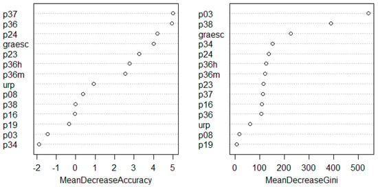
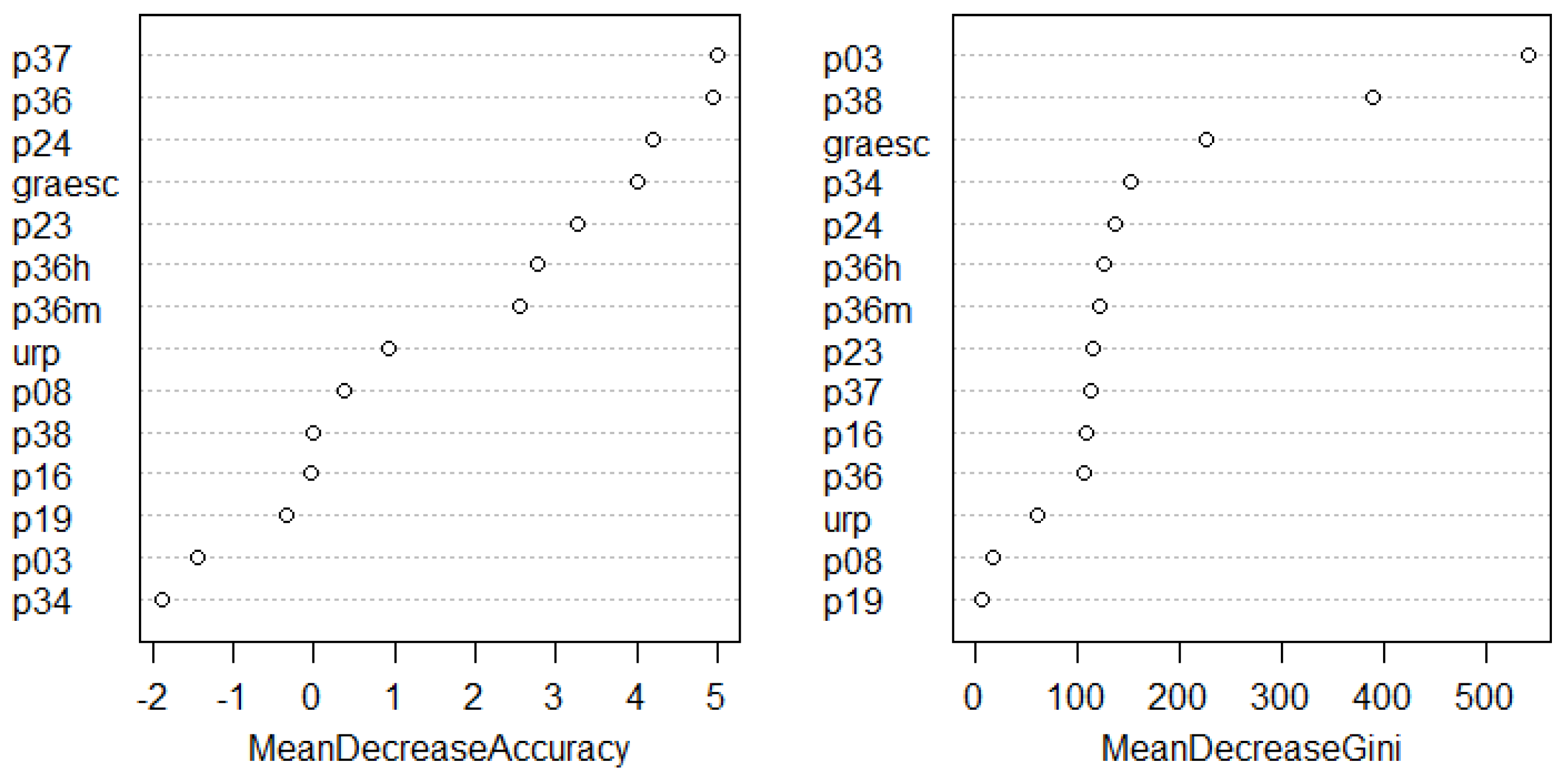
Before imputation, a Random Forest feature-selection stage reduces the original census description to a smaller predictor set relevant to education and fertility. The most influential variables are p24 (highest grade completed), p23 (highest educational level attended), p03 (age), and p38 (age at first child), which are consistent with the interpretation of the problem. The ranking used to define the reduced feature set is shown in Figure 1.

Figure 1. Random Forest ranking used to define the reduced feature set.

In the original manuscript, the feature-selection stage started from a much larger census description and reduced it to a compact analytical representation. The purpose of this stage was twofold: to avoid unnecessary dimensionality during clustering and to preserve only those variables that were substantively related to educational attainment. Variables such as province and sex were not part of the ranking because they had already been used to define the analytical subset. The resulting reduced dataset retained the variables most relevant to schooling grade, fertility history, and local context.

The selected predictors combine educational trajectory, demographic life cycle, and reproductive history. This combination is relevant because graesc is not determined by a single attribute. Age alone cannot recover the target, nor can the educational variables if they are interpreted without accounting for cohort differences or family trajectory. The reduced set therefore preserves descriptors that are both predictive and substantively interpretable.

The original experiments also used Random Forest to examine the relationship between predictive stability and the number of trees. That diagnostic showed that the classification error stabilizes rapidly and that the ranking is dominated by a small set of variables. The ranking procedure and the final supervised imputation stage were not identical: the ranking was first used to identify the most informative variables and reduce dimensionality, and the imputation models were then trained on the reduced dataset. In the original experiments, this strategy produced a compact working representation that preserved high predictive performance while reducing the computational burden of the later clustering and classification stages.

We chose to train the models using only complete observations, ensuring that the predictive power obtained depended exclusively on the observed information and not on previously estimated values. To this end, we applied a two-stage strategy for handling missing data: (i) pairwise deletion, used during the exploratory data analysis and the evaluation of relationships between variables, allowing us to make the most of the available information in each comparison, and (ii) listwise deletion, applied subsequently to form the final training set, considering only those observations that had complete values for the selected predictor variables described in Table 4 and the target variable.

Table 4. Most and least influential variables identified by the Random Forest ranking.

Position in Ranking	Variable and Interpretation
1	p24: highest grade completed
2	p23: highest educational level attended
3	p38: age at first child
4	p03: age
Lower importance	urp: urban/rural area
Lower importance	p19: literacy status
Lower importance	p08: permanent disability for more than one year

Categorical predictors were transformed into a numerical representation, through one-hot coding (also known as creating dummy variables), when required by the clustering stage. In practice, this means that the SOM was trained on a numerically encoded representation of the census records rather than on raw labels. This transformation is not merely an implementation detail. It allows the clustering stage to use mixed demographic information while preserving meaningful proximities between records with similar educational and fertility profiles.

3.3. Construction of the Evaluation Dataset

After variable selection, the reduced dataset was converted into the evaluation dataset used for all imputation experiments which are shown in Table 5. The objective at this stage was to simulate a controlled missing-data problem over a subset for which the true values were still known. To do so, 20% of the observed graesc values were removed at random and treated as missing only during the imputation process. This masking strategy yielded a common test bed for all methods and all clustering configurations.

Table 5. Evaluation dataset used in the imputation experiments.

Property	Value
Total selected attributes	22
Total observations	60,662
Masked values of graesc	12,132
Target variable type	Ordered categorical
Validation strategy	Comparison against original census values

The evaluation dataset therefore contains two versions of the target variable: the temporarily masked version used by the imputers and the original version used for validation. This setup makes it possible to compare the imputed values directly with the true census records. Although this approach does not reproduce every real missingness mechanism, it provides a transparent protocol for comparing methods under identical conditions.

3.4. Target Variable Characterization

The target variable graesc summarizes approved schooling grade. In the original data, it ranges from low schooling values to advanced educational levels, and its distribution is far from uniform. This makes the imputation problem nontrivial: a naive imputer can easily drift toward frequent categories and obscure the educational structure needed for the later mortality analysis.

The original exploratory analysis reported the following summary values for the target variable in the evaluation setting: minimum value 1, maximum value 25, median 11, mode 8, and 12,132 missing values after artificial masking. These summary statistics clarify why the statistical baselines remain weak. Both the median and the mode compress a variable whose distribution reflects heterogeneous educational trajectories across the analytical population.

The evaluation compares six imputers: median, mode, hot-deck, kNN, decision tree, and Random Forest. Each one is applied under three configurations:

1.

Full dataset without previous clustering.

2.

Manual clustering based on canton of residence.

3.

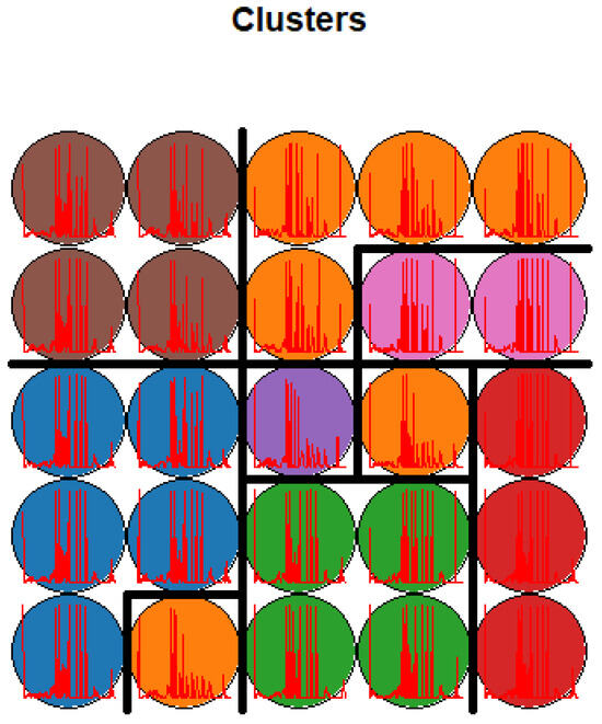
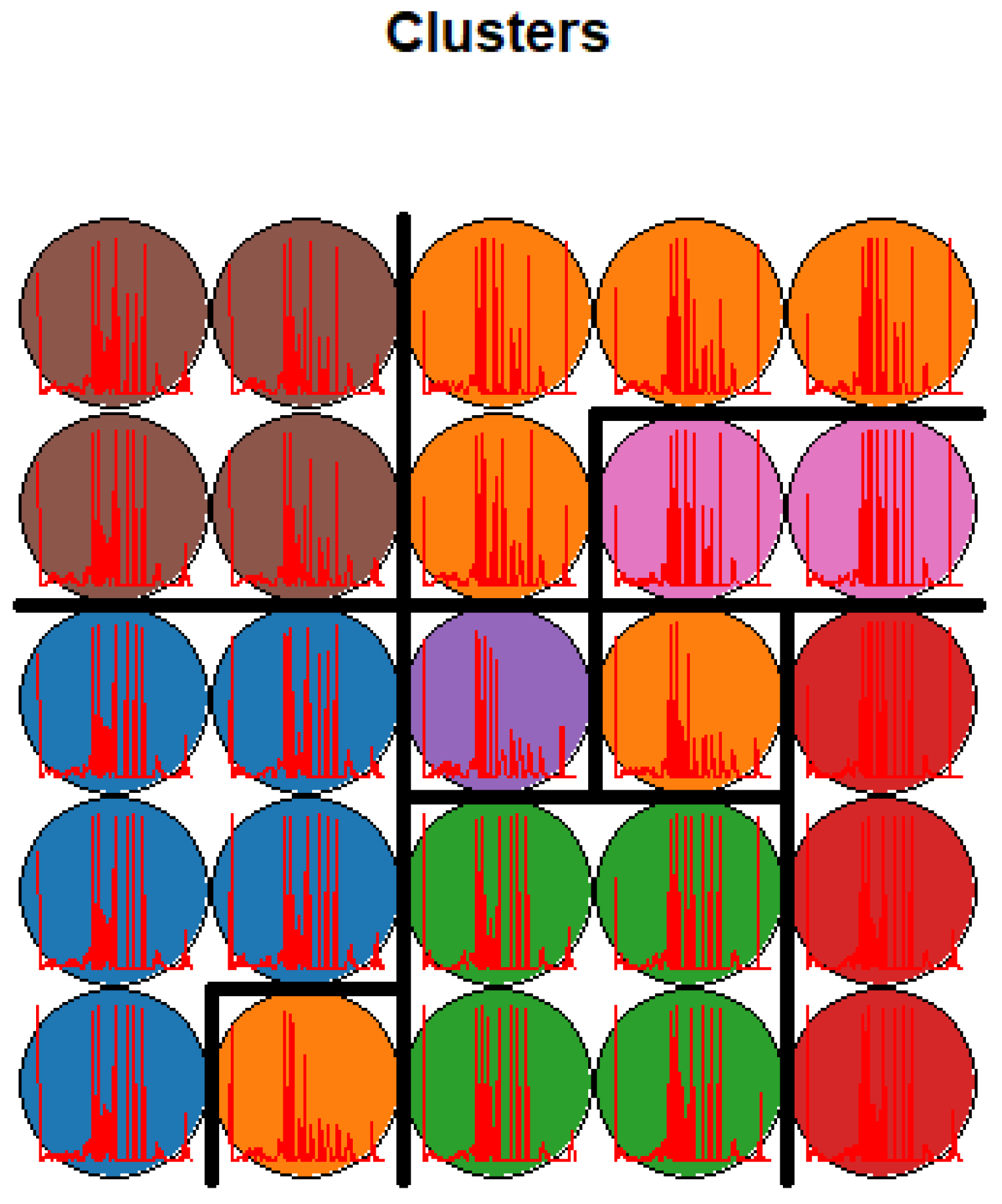
Automatic clustering using a 5 × 5 SOM followed by hierarchical grouping of the codebook into seven clusters.

These three configurations answer different questions. The full-dataset setting serves as the baseline that ignores internal heterogeneity. Manual clustering tests whether a simple administrative partition already captures enough structure to improve prediction. Automatic clustering tests the stronger claim that groups should be learned from the variables themselves and then used as local contexts for imputation.

The proposed workflow is summarized in Algorithm 1. Its central idea is to preprocess the data, select relevant variables, generate homogeneous groups, and impute within each group instead of treating the entire population as a single block.

Algorithm 1 Compact version of the proposed imputation workflow.

Input: preprocessed census dataset

Output: imputed values for graesc

1:  Select relevant predictors

2:  Generate homogeneous clusters

3:  for each cluster do

4:  Train the selected imputation model

5:  Impute missing graesc values

6:  end for

7:  Aggregate the imputed clusters into a final dataset

3.5. Validation Protocol

Artificial masking of observed values provides a direct way to compare predicted and true categories under the same sample conditions. The experiment removes 20% of the observed graesc labels and treats them as missing only during model fitting and prediction. Accuracy is then computed as the percentage of masked cases for which the imputed category matches the original census value. In compact form,

$$\mathrm{Accuracy}={\displaystyle \frac{\mathrm{correct}\mathrm{imputations}}{\mathrm{masked}\mathrm{values}}}\times 100.$$

(1)

This protocol does not aim to reproduce every real-world missingness mechanism. Its purpose is narrower: all candidate methods are evaluated on the same hidden labels, which makes their relative performance directly comparable. This is sufficient for selecting the best imputer within the scope of this study.

The same logic applies to the comparison between clustering strategies. Because the hidden labels are fixed, any improvement observed after manual or automatic clustering can be attributed to the change in representation rather than to a change in the validation sample. This is one of the reasons why the original experiments were organized around the same masked target values across all settings.

3.6. Clustering Design

The SOM-based stage maps observations onto a 5 × 5 grid and then merges the codebook vectors into seven clusters using hierarchical clustering. The map serves as a nonlinear projection that preserves neighborhood relations among observations with similar census profiles. Hierarchical aggregation is then used to avoid treating each SOM cell as an isolated microgroup. The resulting partition retains the advantages of local structure while producing groups large enough for stable imputation.

The SOM was configured with a rectangular 5 × 5 topology, 100 training iterations, and a learning rate decreasing from 0.05 to 0.01, described in Table 6. These values are not presented as universally optimal hyperparameters; rather, they are the settings that produced a stable and interpretable partition in the present data. A larger grid would create more local detail but also more fragmentation, whereas a smaller one would oversmooth the internal heterogeneity that the method is intended to capture.

Table 6. SOM configuration and aggregation choices used in the automatic clustering stage.

Component	Setting
Grid topology	Rectangular
Grid size	5 × 5
Training iterations	100
Learning rate	0.05 to 0.01
Initial map units	25
Final hierarchical clusters	7

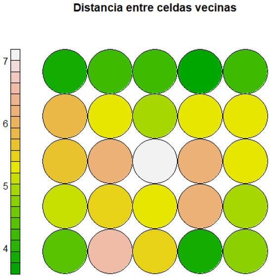
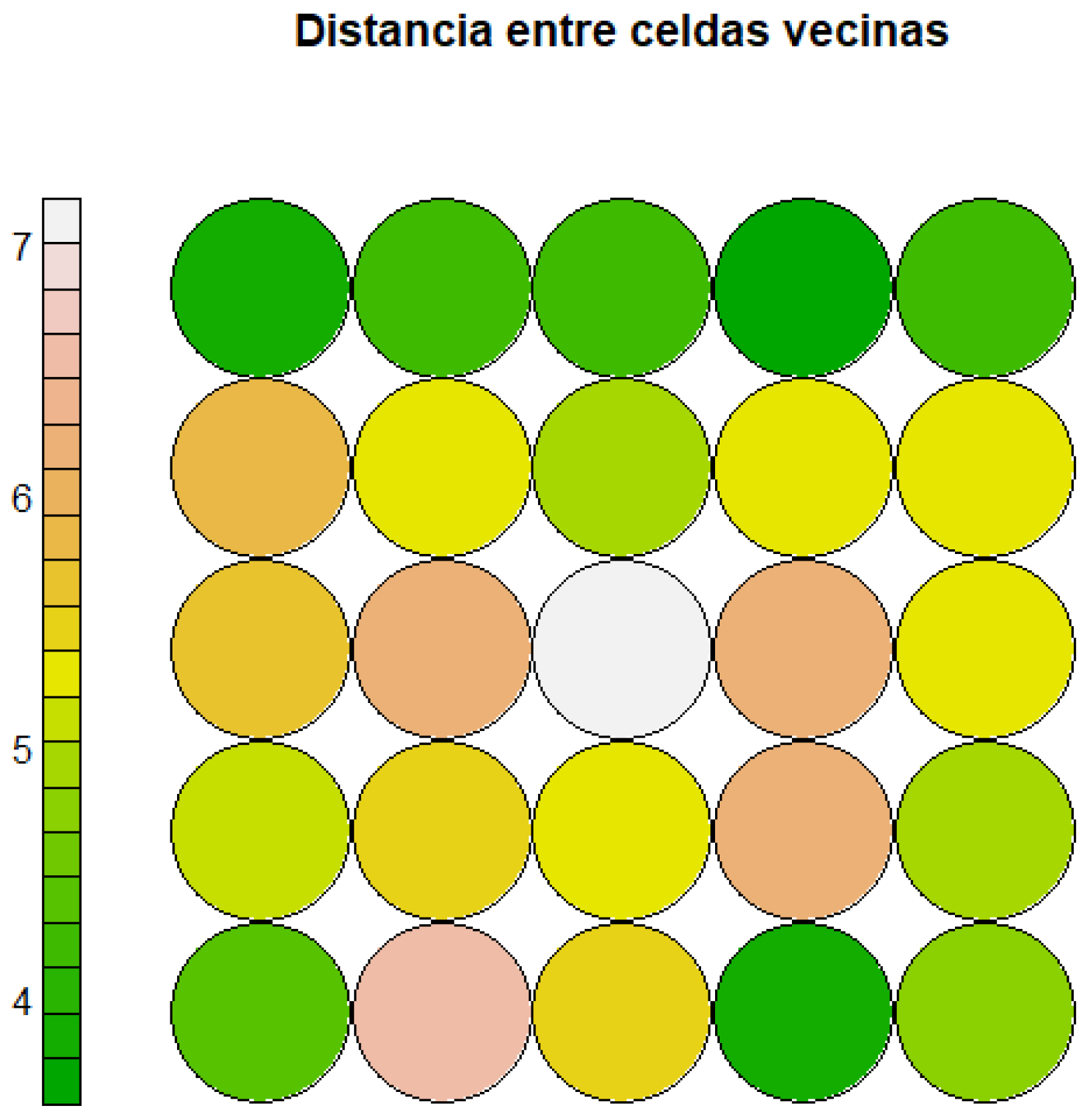
This design differs from manual clustering in an important way. Cantons summarize territory, but they do not necessarily align with educational trajectories, parity, or age-at-childbearing profiles. The SOM groups are built directly from those variables and are therefore expected to be more homogeneous from the perspective of the imputation task. The distance map in Figure 2 illustrates the nonuniform structure learned by the SOM before hierarchical aggregation.

Figure 2. SOM distance map used to identify neighborhoods with different internal dissimilarity before hierarchical grouping.

The 25 SOM cells are also uneven in size, as can be seen in Table 7, which is another indication that the population is not uniformly distributed in predictor space. Some cells concentrate many observations, whereas others capture narrower profiles. This uneven occupancy is informative rather than problematic because it reveals where the data naturally concentrate before higher-level hierarchical grouping is applied.

Table 7. Distribution of observations across the 25 SOM cells.

Cell	Observations	Cell	Observations
1	4992	14	2137
2	1360	15	1835
3	2146	16	2883
4	2406	17	1225
5	4803	18	1321
6	3039	19	2171
7	1230	20	225
8	1855	21	4968
9	1778	22	2732
10	2081	23	2460
11	3483	24	2111
12	838	25	3701
13	851

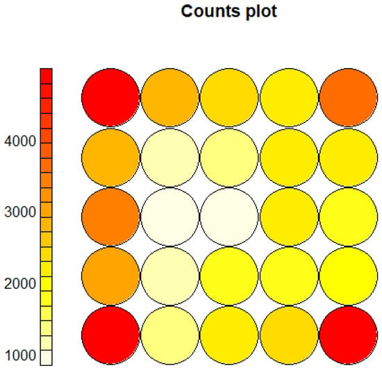
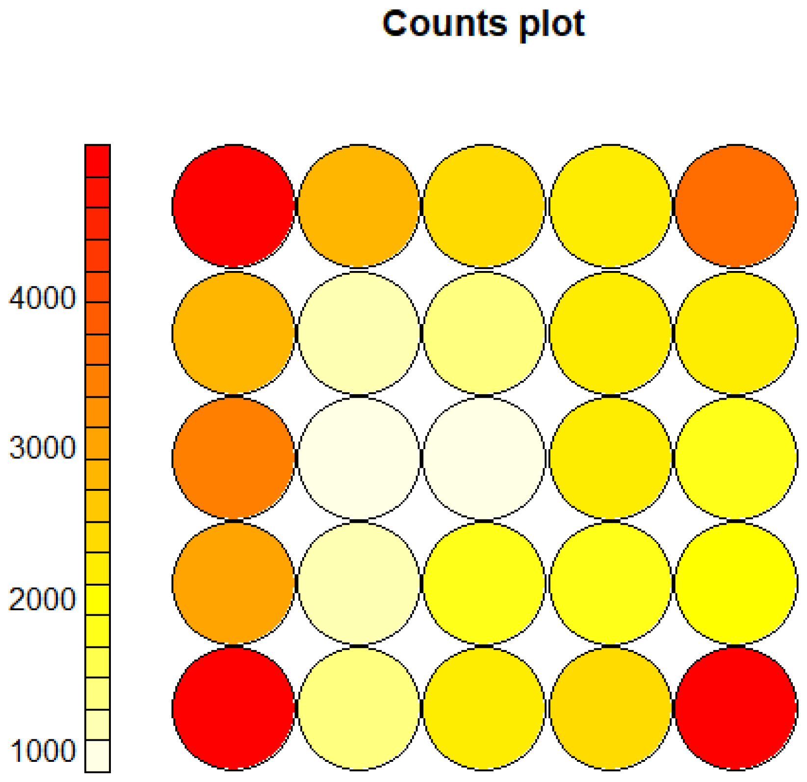
The original SOM experiment reported a heterogeneous allocation of observations across the 25 cells. Some cells contained close to five thousand records, whereas others contained fewer than one thousand. This nonuniform occupancy supports the argument that the full dataset contains internal structure that is not well approximated by a single global imputation model. In that sense, the SOM does not simply partition the data; it reveals where the population is dense, sparse, or structurally differentiated in the predictor space.

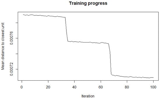
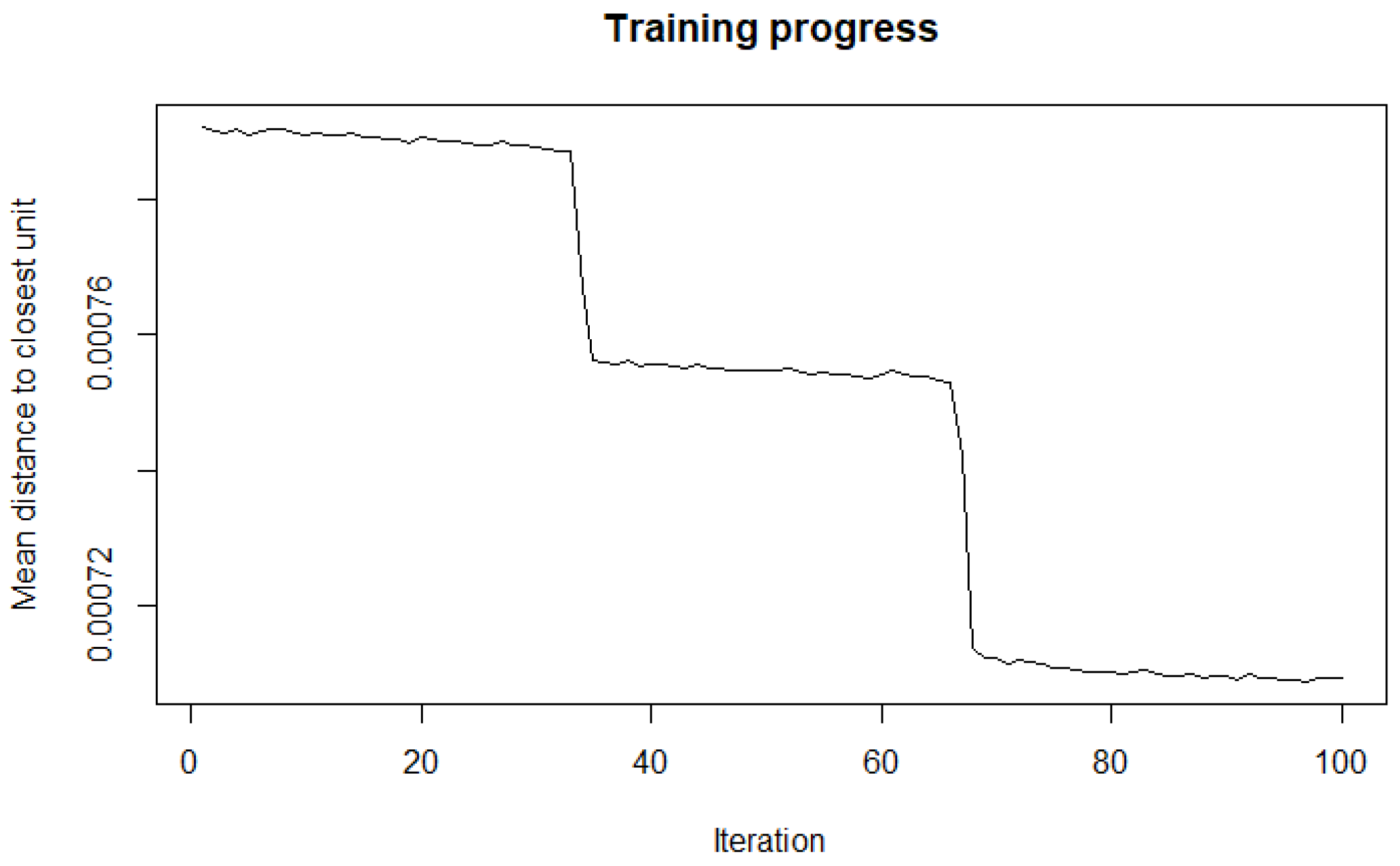
The training process was also monitored to verify that the map converged toward a stable configuration. In the original experiments, the mean distance between each cell and its neighbors decreased as training progressed, as can be seen in Figure 3, eventually reaching a plateau. This behavior is consistent with a stable topological organization, displayed in Figure 2 and supports the use of the trained map as the basis for the later hierarchical aggregation.

Figure 3. Training progress of the SOM, showing the decrease in mean neighborhood distance across iterations.

3.7. Codebook Aggregation and Choice of Seven Clusters

The SOM itself produces 25 local units, one for each cell of the grid. While this level of granularity is useful for visualization, as shown in the heat map of the Figure 4, it is inconvenient for the later imputation stage because some cells are too small and too local to serve as stable analytical clusters. For this reason, the representative codebook vectors of the 25 cells were grouped again using hierarchical clustering. The result is a second-level representation that preserves the topology learned by the SOM while producing clusters large enough for robust imputation.

Figure 4. SOM count map showing the uneven occupancy of the 25 cells before hierarchical aggregation.

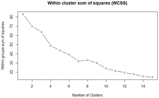
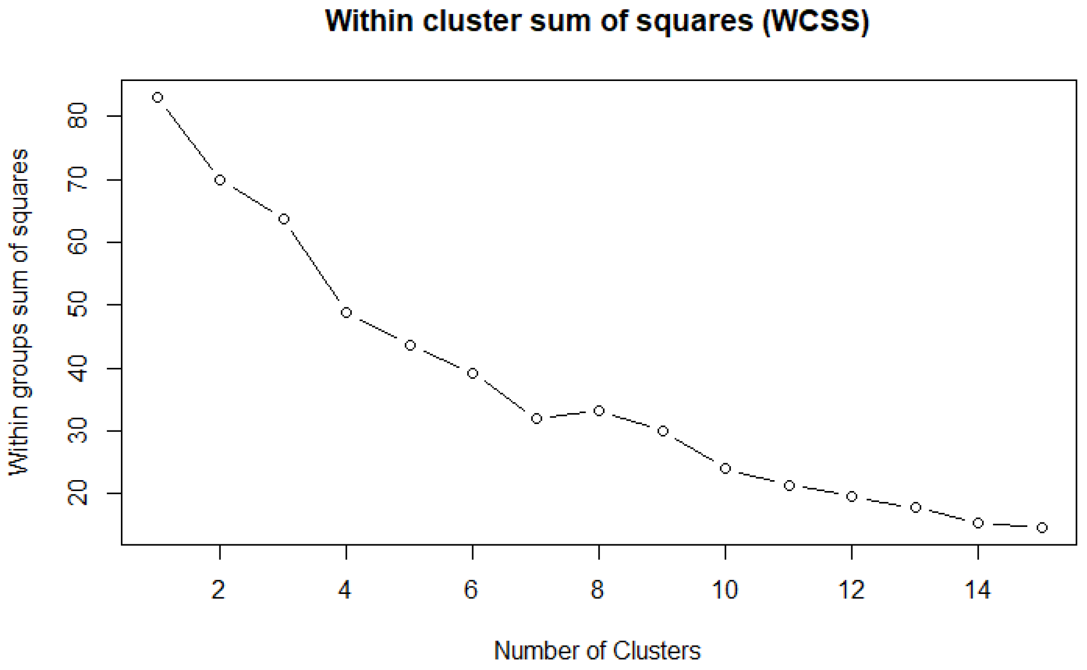
The choice of seven final clusters, as shown in Figure 5, follows the criterion used in the original manuscript: the within-cluster sum of squares (WCSS) stabilizes around that point, visualized in Figure 6. In practical terms, seven clusters represent a compromise between overfragmentation and oversmoothing. Fewer groups would merge clearly distinct census profiles, whereas a much larger number of groups would reproduce the local irregularities of individual SOM cells and reduce the stability of the later classification stage.

Figure 5. Final SOM-hierarchical grouping used before the best-performing imputation stage.

Figure 6. Within-cluster sum of squares used to select seven groups in the hierarchical aggregation of SOM codebook vectors.

The hierarchical aggregation is therefore not an accessory step. It links the descriptive power of the SOM to the operational needs of the imputation stage. By first organizing the data into a topological map and then compressing that map into seven broader groups, the workflow produces clusters that are interpretable, sufficiently populated, and better aligned with the target structure than the original administrative partition.

3.8. Methods Compared

The six imputers span a representative range of complexity. Median and mode provide simple single-value baselines. Hot-deck preserves realism by copying observed values from similar units, but its quality depends on how similarity is defined. kNN can adapt better to local neighborhoods, although it may perform poorly when the predictor space is highly heterogeneous. Decision trees generate explicit partitions of the predictor space and are often effective for mixed demographic variables. Random Forest extends that idea by averaging many trees, which usually improves stability and predictive power [16].

The comparison is intentionally asymmetric. Statistical baselines are included because they remain common in practice, not because they are expected to outperform the supervised models. The main analytical question is whether clustering changes the relative ordering of the methods and whether the gain is large enough to justify the additional preprocessing stage.

3.9. Cluster-Level Readout

The global comparison is sufficient to identify the best overall strategy, but it does not show how performance varies across the learned groups. The cluster-level view is informative because it reveals whether the global gain comes from one dominant cluster or from a broader improvement pattern. In the original experiments, the best SOM-hierarchical configuration improved performance across several clusters simultaneously, especially for the tree-based models.

4. Results

The main result is that clustering before imputation improves accuracy, and automatic SOM-hierarchical clustering is more effective than manual geographic clustering for most methods. Table 8 condenses the full experimental section into a single comparison.

Table 8. Imputation accuracy (%) under the three evaluation settings.

Method	Full Dataset	Manual Clusters	SOM-Hierarchical Clusters
Median	7.33	15.46	39.61
Mode	28.26	28.26	39.43
Hot-deck	12.81	13.71	26.34
kNN	38.67	40.66	56.18
Decision Tree	72.21	85.14	85.25
Random Forest	79.98	82.75	87.03

Several conclusions follow directly from these values. First, statistical imputers perform poorly on the full dataset, although they benefit substantially from automatic clustering. Second, supervised methods clearly outperform statistical baselines in every setting. Third, manual geographic partitioning helps, but its effect is limited because place of residence does not fully capture the internal structure of the data. The best overall result is achieved by Random Forest over SOM-hierarchical clusters, with 87.03% accuracy.

The magnitude of the gain is easier to interpret when the clustered settings are expressed as improvements over the full-dataset baseline. Table 9 shows that all methods improve under SOM-hierarchical clustering, although the gains are not uniform.

Table 9. Absolute accuracy gains (percentage points) relative to imputation on the full dataset.

Method	Manual Clusters	SOM-Hierarchical Clusters
Median	+8.13	+32.28
Mode	+0.00	+11.17
Hot-deck	+0.90	+13.53
kNN	+1.99	+17.51
Decision Tree	+12.93	+13.04
Random Forest	+2.77	+7.05

The clustering stage is therefore more than a descriptive tool. It changes the statistical structure seen by the classifier and reduces within-group heterogeneity. The gain is especially notable for median, mode, hot-deck, and kNN, which suggests that local regularity matters even when the imputer itself is simple. Decision trees also improve substantially from the full dataset to clustered settings, while Random Forest remains the strongest and most stable method overall.

Table 10 shows that the gain is not concentrated in a single subgroup. Clusters 2 and 7 are especially easy to impute, whereas clusters 3 to 6 remain more difficult even after automatic grouping. This pattern is analytically useful because it suggests that the final global accuracy results from consistently better local contexts rather than from a single favorable partition. It also helps explain why Random Forest remains the most reliable method: it combines high performance in the easier clusters with stronger robustness in the more ambiguous ones.

Table 10. Accuracy (%) by SOM-hierarchical cluster for the supervised imputers.

Cluster	kNN	Decision Tree	Random Forest
1	48.23	82.22	84.78
2	74.73	94.25	94.80
3	44.54	75.68	78.82
4	45.94	79.52	78.50
5	38.60	79.52	79.54
6	45.10	85.05	89.28
7	98.81	98.81	98.81

Two patterns deserve emphasis. First, manual clustering is helpful mainly for tree-based methods. This suggests that canton-level aggregation contains some relevant contextual information, but not enough to reorganize the full predictor space for simpler imputers. Second, SOM-hierarchical clustering benefits every method, including those that were already competitive on the full dataset. In other words, learned clusters do not merely rescue weak models; they also strengthen the best one.

The contrast between decision trees and Random Forest is also informative. Decision trees gain more from any kind of clustering because they are sensitive to the structure of local partitions. Random Forest starts from a stronger global baseline and therefore shows smaller relative improvements, but it still achieves the highest final accuracy. This combination of strong baseline performance and consistent gains after clustering makes it the most reliable option for the present data.

On the other hand, we can compare the results of applying the algorithms in two general scenarios. The first test performed involves imputing the graesc variable using the complete dataset. Table 11 shows the results of applying imputation using the following classification methods:

Table 11. ML Methods—Full imputation dataset.

Method	Valid	Error	Accuracy (%)
kNN	4533	7599	37.36
Decision Trees	8452	3680	69.67
Random Forest	9283	2849	76.52

Table 12 shows a summary of the results obtained by applying machine learning-based imputation using clustering.

Table 12. ML Methods—Imputation by cluster.

Method	Valid	Error	Accuracy (%)
kNN	4691	7441	40.66
Decision Tree	10,330	1802	85.14
Random Forest	10,004	1304	82.75

An improvement in the results can be seen when applying this strategy.

To connect imputation quality with the substantive application, the imputed dataset was used in a simplified infant mortality analysis by educational level. Here, we retain only the aggregated result needed for interpretation: lower education is associated with higher estimated infant mortality.

Although the mortality section is intentionally abbreviated, the pattern remains consistent: better imputation preserves the stratification needed to observe meaningful educational differences in infant mortality. The estimated infant mortality rate is 0.040 in the low-education group, compared with 0.025 and 0.024 in the medium- and high-education groups, respectively. Once the educational variable is reconstructed with acceptable accuracy, the expected social gradient becomes visible again.

When calculations are performed using data imputed by the mean, the values change. The Table 13 shows only the final IMR for each level; ^(*) the numbers of women, live births, and surviving children do not match. The number of women, as imputed, increases considerably at the medium level.

Table 13. Aggregated infant mortality estimates after imputation, grouped by educational level.

Level	Women	Live Births	Surviving	IMR	Mean *
Low	27,235	89,432	85,821	0.040	0.38
Medium	20,837	46,980	45,791	0.025	0.027
High	12,900	24,693	24,092	0.024	0.016

This point matters methodologically. A poor imputer could flatten the educational distribution by pushing uncertain records toward frequent categories, which would artificially reduce the observed gap between groups. The present results support the opposite outcome: the best-performing imputation strategy retains enough differentiation to keep the mortality comparison interpretable. In demographic applications, preserving that stratification is often more valuable than a small gain in predictive performance considered in isolation [21,22].

The main contribution is not to describe the mortality prediction model in detail, but rather to propose a strategy for imputing missing socioeconomic variables that allows for the construction of more complete and reliable datasets for subsequent demographic analyses, such as that of infant mortality, through the imputation of the graesc variable.

5. Discussion

The experiments support a direct interpretation: clustering is beneficial when it creates groups aligned with the predictors of the missing variable. In census applications, however, missing data are more likely to follow Missing at Random (MAR) or Missing Not at Random (MNAR) mechanisms than a Missing Completely at Random (MCAR) scenario. Consequently, the proposed strategy does not assume that missing values occur completely at random, even though the experimental evaluation was conducted by randomly removing 20% of the target variable values.

Instead, the approach incorporates a preliminary clustering stage based on Self-Organizing Maps (SOM) to identify homogeneous groups of individuals according to their available sociodemographic characteristics. The underlying hypothesis is that individuals belonging to the same cluster share similar educational and socioeconomic patterns, allowing the imputation process to exploit the latent population structure rather than relying solely on global relationships among variables.

This rationale also explains why manual geographic partitioning satisfies this condition only partially, since administrative units may contain women with heterogeneous educational histories and fertility trajectories. In contrast, the SOM-hierarchical strategy is more effective because it forms clusters according to the structure of the relevant predictor variables themselves.

In this context, the generation of homogeneous clusters constitutes a strategy to reduce the bias associated with structural patterns of missing data and mitigate their impact on the imputation process.

The SOM model was applied as a preliminary step in the prediction process, with the aim of identifying homogeneous groups of individuals with similar sociodemographic characteristics. It is important to note that the SOM clusters were constructed using only predictor variables available in the original dataset. The resulting groups represent structural patterns within the population. This strategy allowed the population to be segmented into subgroups with similar profiles, subsequently facilitating the application of specialized predictive models within each group and improving the accuracy of the imputation process.

The results also illustrate why a baseline comparison is necessary. If only Random Forest had been reported, the contribution of clustering might have appeared modest. However, the full set of methods shows that the preprocessing stage changes the problem in a systematic way. Large gains for median, hot-deck, and kNN indicate that the clustered representation is genuinely easier to impute, not merely better matched to one specific classifier.

This finding is consistent with the broader missing-data literature, which repeatedly shows that imputation quality depends not only on the algorithm but also on how much relevant structure is made available before prediction or estimation [7,10]. In the present case, clustering acts as a representation step: it reorganizes the census records into neighborhoods where the relationship between educational attainment, age, fertility, and household context is more regular. From this perspective, the benefit of SOM-hierarchical clustering lies less in geographic segmentation itself than in improving the local statistical geometry of the problem.

There are also practical implications for statistical offices and public-health analysts. A fully automatic clustering stage adds complexity, but it is more readily justified when the downstream task depends on preserving subgroup structure rather than simply filling isolated missing values. In this case, the target application is infant mortality by educational level, but the same logic could apply to labor-market or migration analyses based on incomplete census variables.

Another relevant point is transportability. The proposed workflow may also be applicable to other census subsets, but its exact gains will depend on how stable the association is between the target variable and the predictors retained after preprocessing. Provinces with a different urban–rural mix, school attendance profile, or fertility schedule may not reproduce the same margins of improvement. This does not weaken the present result; rather, it clarifies its scope. The main contribution of the paper is to show that clustering before imputation can materially improve a downstream demographic analysis when the target variable is socially structured and the administrative partition is too coarse.

From an applied perspective, the comparison also suggests a practical decision rule. If computational simplicity and explainability are the main priorities, decision trees over clustered data may already provide a strong compromise. If the main objective is predictive reliability for downstream demographic estimation, Random Forest over SOM-hierarchical clusters is the preferable option for this dataset. This distinction is relevant for institutions that must balance methodological quality against operational constraints.

The study remains limited in two main ways. First, evaluation is based on artificial masking rather than on a verified missing-at-random mechanism. Second, the paper focuses on a single province and one target categorical variable. These limitations do not invalidate the comparison, but they do narrow its external generality. The main conclusion should therefore be read as a well-supported result for this census subset rather than as a universal rule for all official statistics.

Two further limitations should also be noted. First, the study evaluates accuracy at the imputation stage but does not perform a full sensitivity analysis of how alternative completed datasets would affect the final infant mortality estimates. Second, the clustering hyperparameters were selected for stability and interpretability rather than optimized through an extensive search. Both points are natural directions for future work, especially if the methodology is to be operationalized in repeated census-processing pipelines.

6. Conclusions

This study shows that imputing graesc after automatic SOM-hierarchical clustering yields better results than imputing on the full dataset or after manual geographic partitioning. The advantage is strongest for Random Forest, which reaches 87.03% accuracy, while decision trees also remain highly competitive.

Two conclusions follow. First, cluster generation is a useful preprocessing stage for categorical imputation in large demographic datasets. Second, the gain in imputation quality improves the reliability of downstream public-health indicators, illustrated here through infant mortality by educational level.

While approaches based on satellite imagery and deep learning spatial models have demonstrated the ability to reconstruct population distribution patterns at regional scales, these methods generally operate on aggregated units [23]. In contrast, this study addresses the reconstruction of socioeconomic information at the individual level using a hybrid framework that combines unsupervised and supervised learning, thereby capitalizing on the heterogeneity within the population.

Future work should validate the same strategy in additional census regions and for other missing categorical variables, and should compare SOM-based clustering with alternative representation-learning approaches.

References

- Lazcano-Ponce, E.; Schiavon, R.; Uribe-Zúñiga, P.; Walker, D.; Suárez-López, L.; Luna-Gordillo, R.; Ulloa-Aguirre, A. Cobertura de atención del parto en México: Su interpretación en el contexto de la mortalidad materna. Salud Pública Méx. 2013, 55, S214–S224. [Google Scholar] [CrossRef] [Scilit]
- Chackiel, J. Métodos de estimaciones demográficas de pueblos indígenas a partir de censos de población: La Fecundidad y la Mortalidad. In Pueblos Indigenas y Afrodescendientes de América Latina y el Caribe: Relevancia y Pertinencia de la Informacion Sociodemografica para Politicas y Programas; ECLAC: Santiago, Chile, 2005; p. 30. [Google Scholar]
- Acuña, M. Redatam Informa. Redatam Inf. 2013, 13. [Google Scholar]
- Torres, V.E.R.; Bertone, C.L.; Andrada, M.J. Brechas en la mortalidad infantil según nivel educativo de las madres en la Provincia de Córdoba. Estimación indirecta a partir de datos censales 2010. Rev. Salud Pública 2018, 22, 37–47. [Google Scholar] [CrossRef] [Scilit]
- Rubin, D.B. Inference and missing data. Biometrika 1975, 63, 581–592. [Google Scholar] [CrossRef] [Scilit] [PubMed]
- Rubin, D.B. Multiple imputation after 18+ years. J. Am. Stat. Assoc. 1996, 91, 473–489. [Google Scholar] [CrossRef]
- Little, R.J.A.; Rubin, D.B. Statistical Analysis with Missing Data, 3rd ed.; Wiley: Hoboken, NJ, USA, 2019. [Google Scholar]
- Cheema, J.R. A review of missing data handling methods in education research. Rev. Educ. Res. 2014, 84, 487–508. [Google Scholar] [CrossRef] [Scilit]
- Bar, H. Missing data—Mechanisms and possible solutions. Cult. Educ. 2017, 29, 492–525. [Google Scholar] [CrossRef] [Scilit]
- Sterne, J.A.C.; White, I.R.; Carlin, J.B.; Spratt, M.; Royston, P.; Kenward, M.G.; Wood, A.M.; Carpenter, J.R. Multiple imputation for missing data in epidemiological and clinical research: Potential and pitfalls. BMJ 2009, 338, b2393. [Google Scholar] [CrossRef] [Scilit] [PubMed]
- Andridge, R.R.; Little, R.J. A review of hot deck imputation for survey non-response. Int. Stat. Rev. 2010, 78, 40–64. [Google Scholar] [CrossRef] [Scilit] [PubMed]
- Myers, T.A. Goodbye, listwise deletion: Presenting hot deck imputation as an easy and effective tool for handling missing data. Commun. Methods Meas. 2011, 5, 297–310. [Google Scholar] [CrossRef] [Scilit]
- García-Laencina, P.J.; Sancho-Gómez, J.L.; Figueiras-Vidal, A.R.; Verleysen, M. K nearest neighbours with mutual information for simultaneous classification and missing data imputation. Neurocomputing 2009, 72, 1483–1493. [Google Scholar] [CrossRef] [Scilit]
- Rahman, M.G.; Islam, M.Z. A decision tree-based missing value imputation technique for data pre-processing. Conf. Res. Pract. Inf. Technol. Ser. 2010, 121, 41–50. [Google Scholar]
- Genuer, R.; Poggi, J.M.; Tuleau-Malot, C. Variable selection using random forests. Pattern Recognit. Lett. 2010, 31, 2225–2236. [Google Scholar] [CrossRef] [Scilit]
- Svetnik, V.; Liaw, A.; Tong, C.; Culberson, J.C.; Sheridan, R.P.; Feuston, B.P. Random forest: A classification and regression tool for compound classification and QSAR modeling. J. Chem. Inf. Comput. Sci. 2003, 43, 1947–1958. [Google Scholar] [CrossRef] [Scilit] [PubMed]
- Fessant, F.; Midenet, S. Self-organising map for data imputation and correction in surveys. Neural Comput. Appl. 2002, 10, 300–310. [Google Scholar] [CrossRef] [Scilit]
- Ruiz-Chavez, Z.; Salvador-Meneses, J.; Garcia-Rodriguez, J. Machine Learning Methods Based Preprocessing to Improve Categorical Data Classification. In Proceedings of the International Conference on Intelligent Data Engineering and Automated Learning; Springer: Berlin/Heidelberg, Germany, 2018; pp. 297–304. [Google Scholar]
- Jiang, S.; Chin, K.S.; Wang, L.; Qu, G.; Tsui, K.L. Modified genetic algorithm-based feature selection combined with pre-trained deep neural network for demand forecasting in outpatient department. Expert Syst. Appl. 2017, 82, 216–230. [Google Scholar] [CrossRef] [Scilit]
- Kefale, B.; Jancey, J.; Gebremedhin, A.T.; Nyadanu, S.D.; Belay, D.G.; Pereira, G.; Tessema, G.A. Risk factors of under-five and infant mortality: An umbrella review of systematic reviews and meta-analyses. J. Glob. Health 2024, 14, 04260. [Google Scholar] [CrossRef] [Scilit] [PubMed]
- Coale, A.J.; Trussell, T.J. Model fertility schedules: Variations in the age structure of childbearing in human populations. Popul. Index 1974, 40, 185–258. [Google Scholar] [CrossRef] [Scilit]
- Trussell, T.J. A re-estimation of the multiplying factors for the Brass technique for determining childhood survivorship rates. Popul. Stud. 1975, 29, 97–107. [Google Scholar] [CrossRef] [Scilit] [PubMed]
- Zhuang, H.; Liu, X.; Yan, Y.; Ou, J.; He, J.; Wu, C. Mapping multi-temporal population distribution in China from 1985 to 2010 using landsat images via deep learning. Remote Sens. 2021, 13, 3533. [Google Scholar] [CrossRef] [Scilit]
Disclaimer/Publisher’s Note: The statements, opinions and data contained in all publications are solely those of the individual author(s) and contributor(s) and not of MDPI and/or the editor(s). MDPI and/or the editor(s) disclaim responsibility for any injury to people or property resulting from any ideas, methods, instructions or products referred to in the content. |
© 2026 by the authors. Licensee MDPI, Basel, Switzerland. This article is an open access article distributed under the terms and conditions of the Creative Commons Attribution (CC BY) license.