


Abstract
A Monte Carlo method for the modeling of traffic in a network is developed. The main advantage of the method is the possibility of using arbitrary probability functions for the transfer of an element of the flow to the next node. The model is validated by comparison with results known from the literature. Possible applications of the method for modeling in nonlinear and delay systems are discussed.
1. Introduction
Monte Carlo methods are a wide class of numerical methods using random numbers. They are applied in many areas of mathematics, natural sciences and engineering. The current development of computers has increased their application in the modeling of many stochastic and deterministic processes (see, e.g., [1,2]).
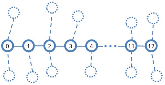
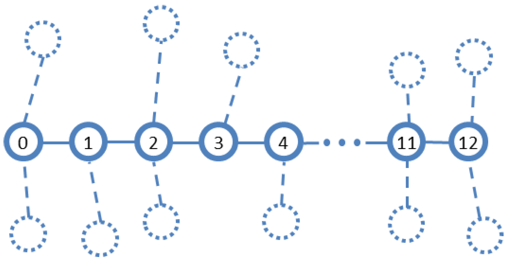
In the current work, a Monte Carlo method is employed for the modeling of traffic in a single-arm channel in a network (Figure 1). The substance enters the 0-node and, with some probability, moves to the next node of the channel or to nodes not belonging to it. The substance cannot enter the channel from nodes that are not part of it. The motion of the substance in the channel and the more general cases of an infinite channel or a channel with an arbitrary number of arms are studied in detail in [3,4,5].
Figure 1.
Part of the network modeled in the paper. The nodes of the channel, numbered from 0 to 12, are represented by solid circles, and the edges that connect the nodes are represented by solid lines. Other nodes and edges of the network are marked by dashed or dotted lines.
The aim of our study is to test the developed Monte Carlo method in some cases of the above-described network. First, the method is validated by comparison with results known from the literature. Then it is applied to nonlinear systems with a probability of transfer depending on the amount of substance in a node. The third test is with a delay system, in which the probability of transfer is a function of the time spent by the substance in a node.
2. Description of the Method
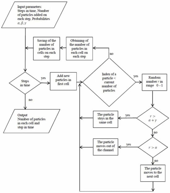
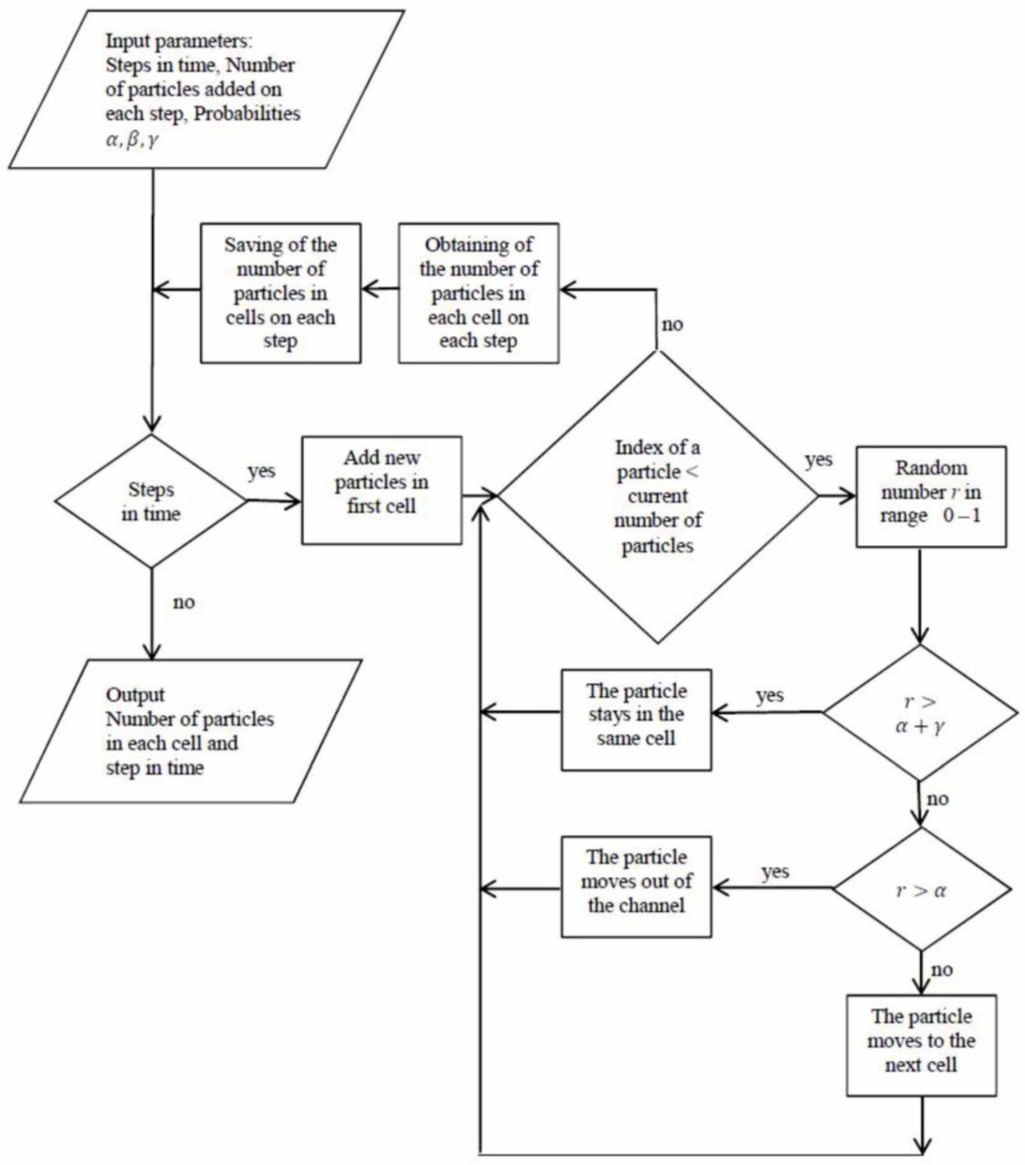
The continuous process is discretized into small time steps (Figure 2). The substance in the channel is also presented as a flow of discrete elements, called here particles. The number of particles in each node of the network at the beginning is zero. Then new particles start to enter the zero node of the network. In the present work, the number of particles entering the network at each time step is constant, but the method permits arbitrary time variation of their number. During one time step, every particle in a node of the network can stay in the same node, move to the next node in the channel, or move outside the channel into the external environment.
Figure 2.
Flowchart of the Monte Carlo algorithm for modeling of flow in a network channel.
The probabilities αi and γi for the transfer of a particle from the i-th node to the next node and for leakage outside the channel during the time step are external parameters. A random number r01 uniformly distributed between 0 and 1 is generated for each particle in a node. If r01 < αi, the particle is moved to the next cell of the channel; if αi < r01 < αi + γi, the particle is moved outside the channel and leaves the simulation; and if αi + γi < r01, the particle stays in the same node. The procedure is repeated for all particles in every time step. After reaching a quasi-stationary state, the data for the number of particles in each node are collected and averaged in time.
3. Validation of the Model
The Monte Carlo model is validated by comparison with the results in [3] using the traditional method of solving the problem with a system of differential equations:
Here is the amount of substance (the number of particles in the Monte Carlo model) in the i-th node. The first term on the right-hand side gives the particle transfer from the previous node, the second term represents the losses to the next node, and the leakage from the channel. There is an extra term with β in Equation (1) [3] giving an additional probability of transfer to the next node. In the Monte Carlo model, it is treated in the same manner as αi.
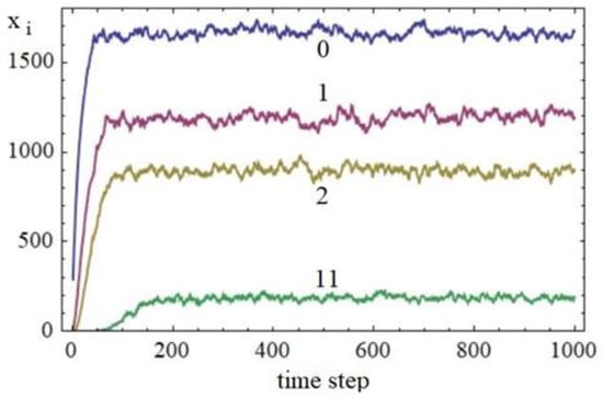
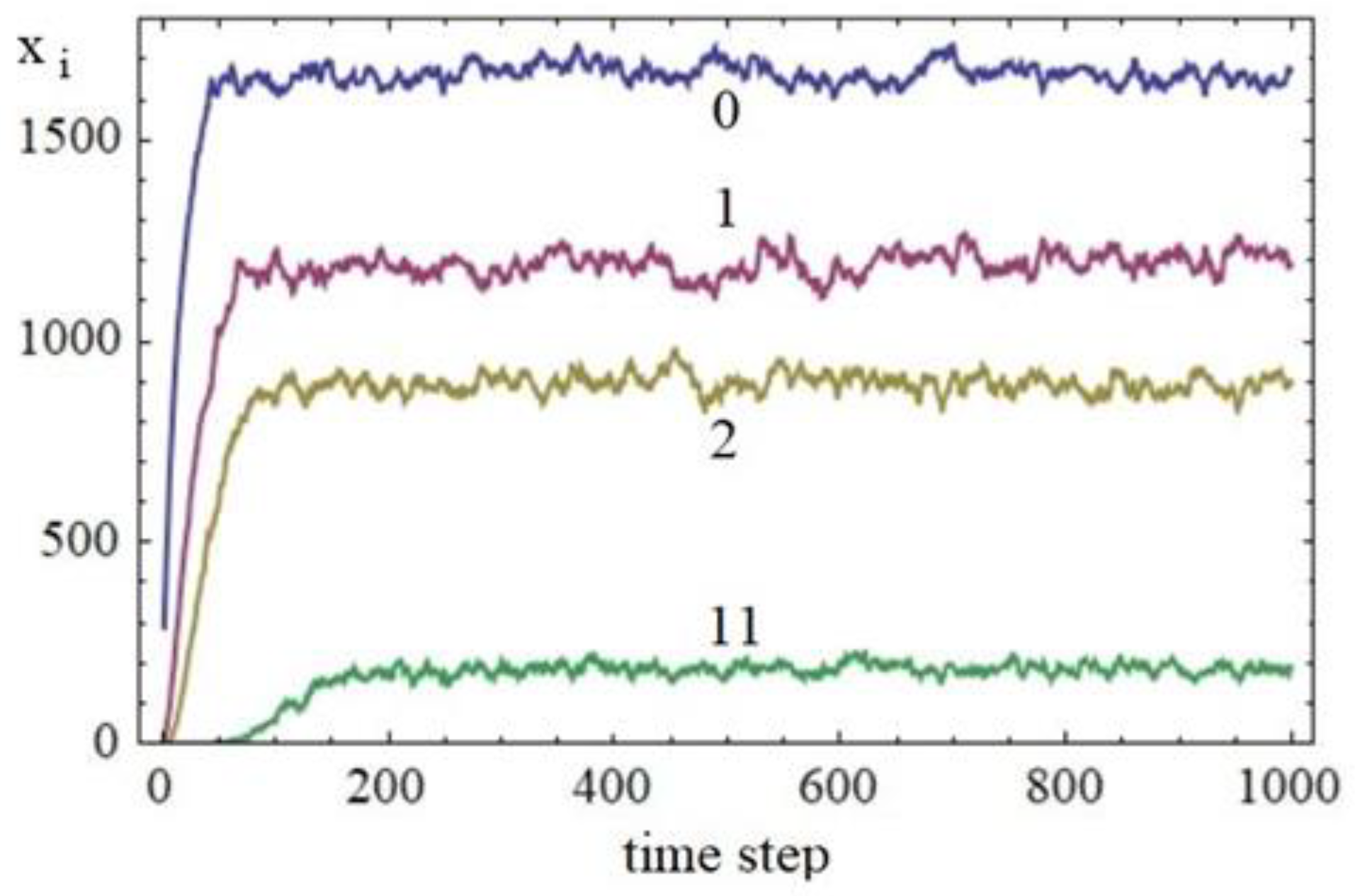
The values of the parameters are as follows: α = 0.05, β = 0.01 and γ = 0.01. The number of particles entering the zero node at each time step is 100 and the total number of steps is 1000 (Figure 3).
Figure 3.
Time dependence of the number of the particles xi in nodes 0, 1, 2 and 11, as designated in the figure.
The quasi-stationary state is reached after about 150 time steps (Figure 3). After averaging the data for steps 200 to 1000 and normalizing them to the value of the zero node, the results are compared with the results from (3).
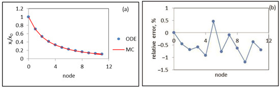
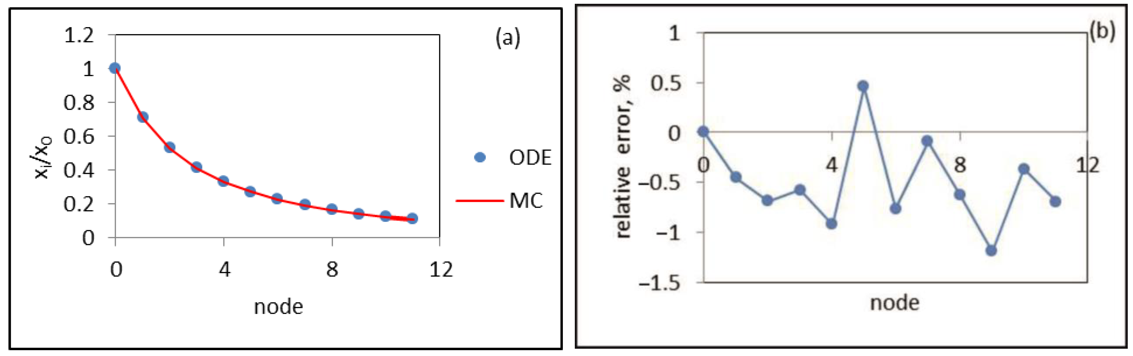
The results in Figure 4 demonstrate that the Monte Carlo method gives correct results. Our tests show—as should be expected—that the accuracy of the results increases with the number of particles.
Figure 4.
Comparison of the results obtained by the Monte Carlo method (line) and system of differential equations (symbols) in (a) and relative error in % in (b).
4. Test Results in Nonlinear Systems
The system of Equation (1) has an analytical solution in the case of constant values of the probabilities α, β and γ [3]. If the probabilities are functions of x, the system is nonlinear, and, in general, an analytical solution does not exist, and even obtaining a numerical solution could be difficult in some cases. The Monte Carlo method could be applied for an arbitrary dependence of the probabilities on x. In this section, two examples of a nonlinear dependence of α on x are presented.
4.1. Example 1. α decreases with x
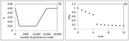
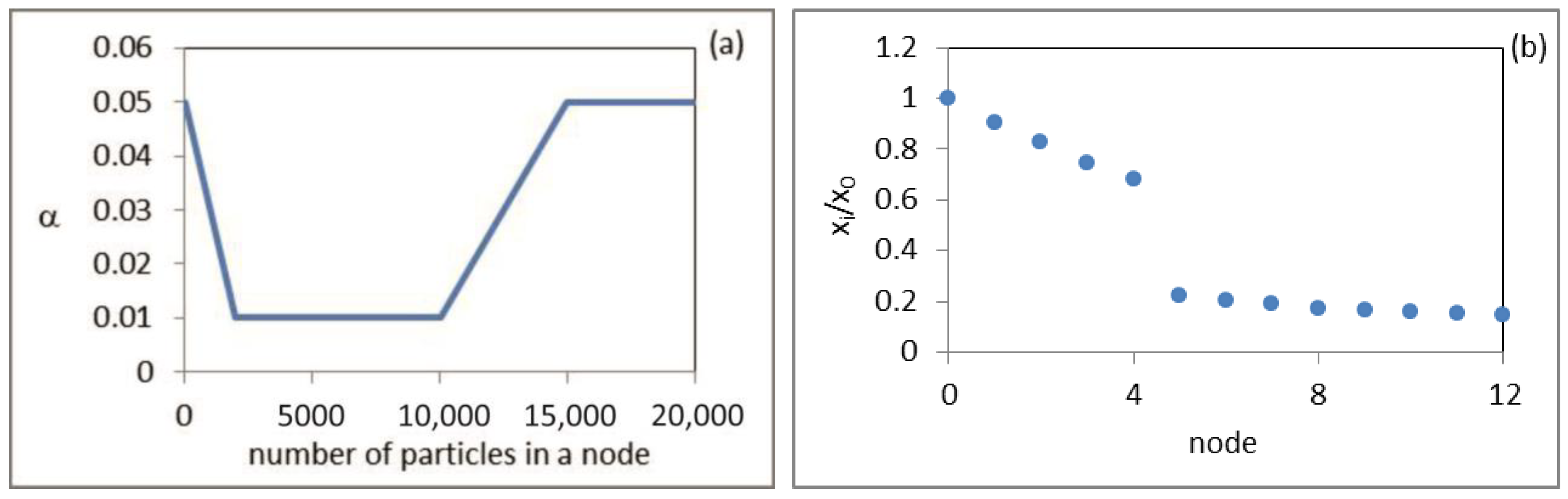
The dependence of α on the number of particles in the node is shown in Figure 5a. α decreases linearly from 0.05 at x = 0 to 0.01 at x = 2000 and then stays constant at this low value. The increase in α at x > 10,000 is not important because in the simulation the values of x are much smaller. The values of the other probabilities are β = 0 and γ = 0.001, i.e., in this case the results are determined mainly by the behavior of α.
Figure 5.
Dependence of α on the number of particles in the node x (a) and results for the normalized number of particles versus the node number (b) for the conditions of example 1.
Results in Figure 5b show two groups of nodes. The first group consists of the first five nodes. The number of particles there is large enough to reach the plateau in Figure 5a between 2000 and 10,000. The probability α is small, and the particles stay in these nodes for a relatively long time. The second group is for nodes 5–12. The probability α is large, the particles leave these nodes fast, and the number of particles is small.
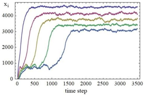
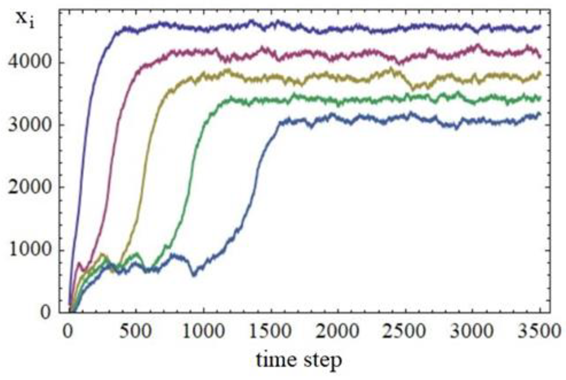
A jump from the second to the first group is visible in Figure 6. Initially, all the nodes are in the second group, i.e., the number of particles is small. With time, particles are transferred from the previous nodes, their number increases, and the probability of loss of a particle to the next node decreases. The number of particles in the node increases fast.
Figure 6.
Time dependence of the number of particles in the first five nodes of the channel. The leftmost curve corresponds to the first node, the second curve from the left corresponds to the second node, and so on.
4.2. Example 2. α increases with x
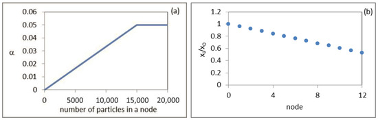
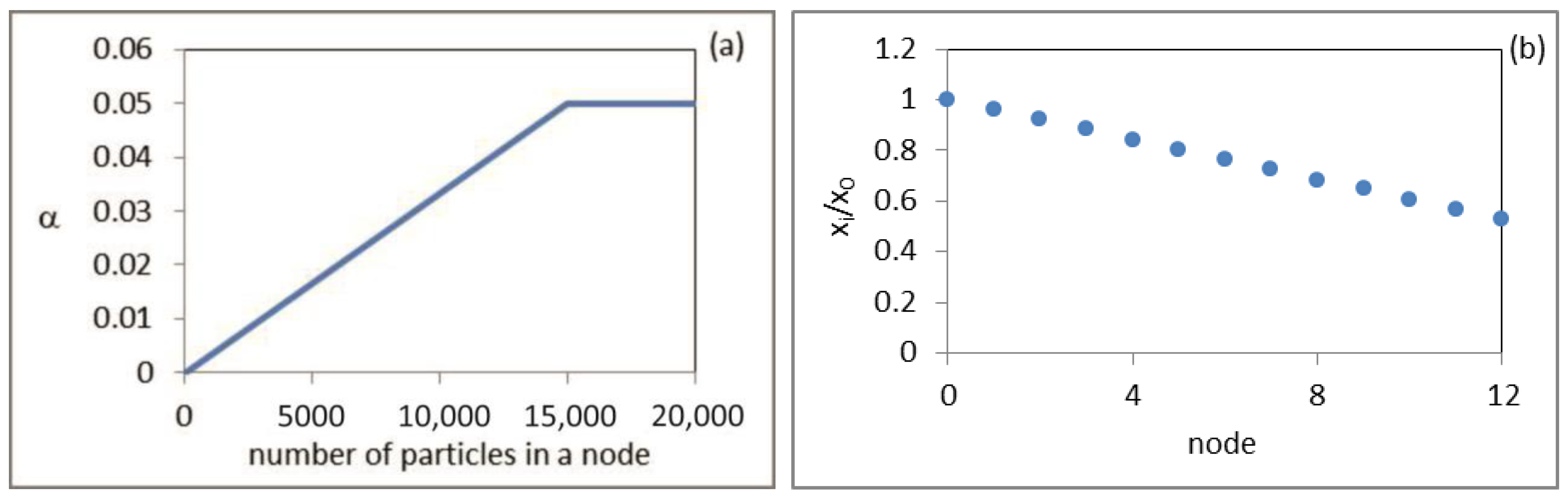
In this case, the probability α increases linearly from 0 to 0.05 (Figure 7a). Above x = 15,000 the value of α is constant, but in the simulation, the values of x are always smaller than 15,000. The values of the other probabilities are β = 0 and γ = 0.001, as in the previous example. In contrast to the case with a constant value of α, where the number of particles in a node decreases exponentially (Figure 4a) here the dependence is linear (Figure 7b). A simple analysis of the system of Equation (1) in this example shows that the number of particles always decreases in the next node by approximately γ/(2 a). (a is the slope of the line in Figure 7a, i.e., a = Δα/Δx). This is confirmed numerically in the simulation. In our case, γ/(2 a) = 150, x0 = 3722, x11 = 2109, x11 − x0 = 1613 while 11γ/(2 a) gives approximately the same value, 1650. Additional tests show that if the value of γ is zero, the profile of the number of particles is a horizontal line with the values of x determined by the number of particles entering the channel at each time step and α.
Figure 7.
Dependence of α on the number of particles in the node x (a) and results for the normalized number of particles versus the node number (b) for the conditions of example 2.
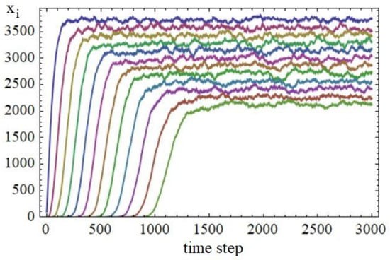
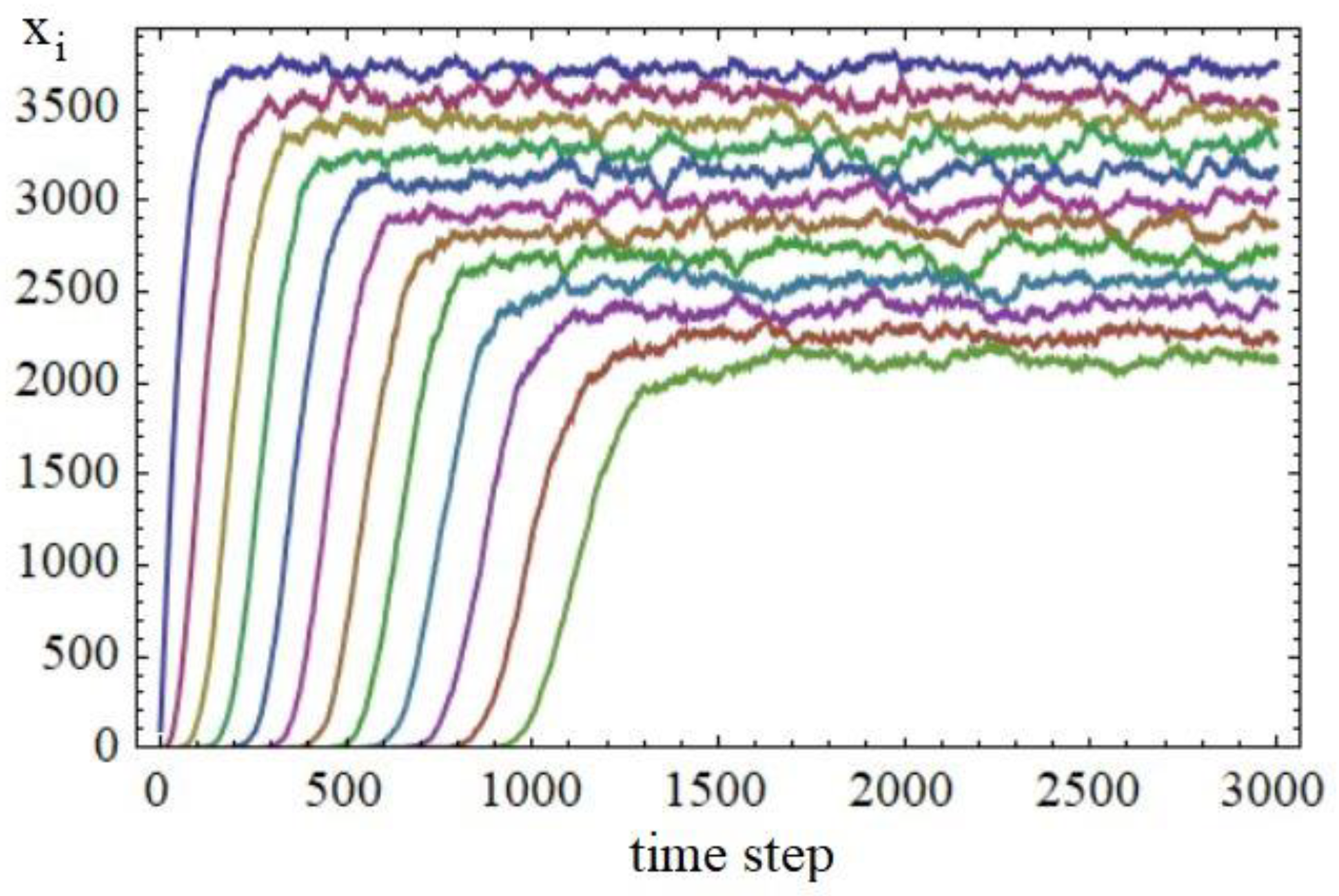
The time dependence of the number of particles in the nodes is shown in Figure 8. The transfer of particles to the i + 1-th node is significant only if the number of particles in the i-th node is large enough and, correspondingly, the probability from Figure 7a is large enough. This is the reason for the shift in time of the profiles for different nodes in Figure 8. With the increase in the node number i the number of particles decreases, and the speed of the transfer also decreases, which explains the smaller slope of the profiles at higher i.
Figure 8.
Time dependence of the number of particles in all twelve nodes of the channel. The leftmost curve corresponds to the first node, the second curve from the left corresponds to the second node, and so on.
5. Test Results in Delay Systems
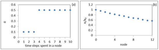
In the next test, the probability for transfer of a particle depends on the time spent by the particle in a given node, which is called its residence time. As an example, the probability of transfer for a newly arrived particle in a node is α = 0.01 for the first 3 time steps and then increases to α = 0.5 (Figure 9a). The values of the other constants are β = 0 and γ = 0.1.
Figure 9.
Dependence of α on the time spent by a particle in the node (a) and results for the normalized number of particles versus the node number (b).
The result for the normalized number of particles in the nodes is shown in Figure 9b. A precise analysis shows that the number of particles decreases exponentially. Since the exponential decay constant is very small, this is not well seen in Figure 9b.
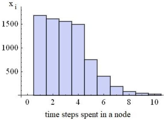
The distribution of the residence time of particles in the nodes is affected in the expected manner by the probabilities in Figure 9a. Results in node 5 are shown here as an example (Figure 10). For small residence times, the probability of transfer is small, and the number of particles decreases mainly due to leakage outside the channel. The jump in probability after four time steps in Figure 9a leads to a fast decrease in the number of particles for longer residence times.
Figure 10.
Number of particles in node 5 as a function of the time steps spent in the node.
6. Conclusions
The tests of the developed Monte Carlo model demonstrate its applicability to the problems of traffic in a network. In the cases with available analytical results, the results obtained by the Monte Carlo method fully coincide with the results of the solution of the system of differential equations. In tests where a direct comparison with other solutions is not possible, the Monte Carlo method gives expected and explainable results.
The method could be used for nonlinear or delay systems where the traditional methods are not effective. Obviously, the method is more appropriate for the traffic of discrete elements.
Our future plans are directed toward the optimization of the algorithm, a systematic study of the role of the parameters in the model, and solving real-world problems instead of the test problems presented in the current work.
Author Contributions
Conceptualization, K.T.; methodology, K.T.; writing—original draft preparation, K.T. and R.A.; writing—review and editing, K.T. and R.A.; supervision, K.T.; K.T. and R.A. contributed equally to this paper. All authors have read and agreed to the published version of the manuscript.
Funding
This research received no external funding.
Institutional Review Board Statement
Not applicable.
Informed Consent Statement
Not applicable.
Data Availability Statement
The raw data supporting the conclusions of this article will be made available by the authors on request.
Acknowledgments
The authors would like to thank the Research and Development Sector at the Technical University of Sofia for the financial support.
Conflicts of Interest
The authors declare no conflicts of interest.
References
- Kalos, M.H.; Whitlock, P.A. Monte Carlo Methods, 2nd ed.; WILEY-VCH Verlag GmbH & Co. KGaA: Weinheim, Germany, 2008; pp. 107–159. [Google Scholar]
- Landau, D.; Binder, K. A Guide to Monte Carlo Simulations in Statistical Physics, 4th ed.; Cambridge University Press: Cambridge, UK, 2014; pp. 1–140. [Google Scholar]
- Vitanov, N.K.; Borisov, R. A model of a motion of substance in a channel of a network. J. Theor. Appl. Mech. 2018, 48, 74–84. [Google Scholar]
- Vitanov, N.K.; Borisov, R. Human migration: Model of a migration channel with a secondary and a tertiary arm. AIP Conf. Proc. 2019, 2075, 150001. [Google Scholar] [CrossRef] [Scilit]
- Borisov, R.; Dimitrova, Z.I.; Vitanov, N.K. Statistical characteristics of stationary flow of substance in a network channel containing arbitrary number of arms. Entropy 2020, 22, 553. [Google Scholar] [CrossRef] [Scilit] [PubMed]
Disclaimer/Publisher’s Note: The statements, opinions and data contained in all publications are solely those of the individual author(s) and contributor(s) and not of MDPI and/or the editor(s). MDPI and/or the editor(s) disclaim responsibility for any injury to people or property resulting from any ideas, methods, instructions or products referred to in the content. |
© 2026 by the authors. Licensee MDPI, Basel, Switzerland. This article is an open access article distributed under the terms and conditions of the Creative Commons Attribution (CC BY) license.