Inverse Copula Sampling for Multi-Dimensional Data Synthesis ^†

Abstract

In the era of big data, the demand for vast quantities of diverse and representative datasets has surged across various domains, from healthcare and finance to artificial intelligence and machine learning. Synthetic data generation offers a promising solution by enabling the creation of data with specific properties that closely mimic real-world data while avoiding privacy concerns and regulatory limitations. However, generating high-quality synthetic data that accurately preserves complex dependencies remains a significant challenge. This paper addresses this gap by exploring a novel approach: Inverse Copula Sampling for Multi-Dimensional Data Synthesis. Utilizing copulas, which are powerful tools for modeling dependencies between variables, our method generates synthetic data that maintains intricate interdependencies. We demonstrate the effectiveness of this approach through various experiments and case studies, showing high fidelity in preserving dependencies and minor discrepancies in marginal distributions. The method’s robustness was validated through comparative analysis and statistical checks, including the Kolmogorov–Smirnov test. Our research contributes to the field by introducing a flexible and efficient method for synthetic data generation that is applicable to a wide range of data distributions and practical applications. Future work will explore the application of other copula types and the further refinement of the method to enhance its versatility.

1. Introduction

In the era of big data, the demand for vast quantities of diverse and representative datasets has surged across various domains, from healthcare and finance to artificial intelligence and machine learning. One promising approach to meet this demand is the use of synthetic data, which refers to data that does not exist in the real world but is generated through algorithms that incorporate statistical dependencies. Synthetic data offers several advantages, such as the absence of privacy concerns and regulatory limitations while preserving the interrelationships among variables. This aspect is particularly crucial in sensitive fields like financial services, where data privacy is paramount. Additionally, synthetic data is cost-effective and timesaving, eliminating the need for extensive data collection and processing efforts. However, the literature lacks a comprehensive investigation into sophisticated methods for generating high-quality synthetic data that accurately represents demographic, financial, psychological, and social-status data. This paper aims to fill this gap by exploring the novel approach of Inverse Copula Sampling for Multi-Dimensional Data Synthesis.

To answer this research question, we propose a method that leverages copulas, powerful statistical tools that model complex dependencies between variables. By using the Inverse Copula Sampling method, we can generate synthetic data that maintains the intricate interdependencies present in multi-dimensional datasets. Our approach benefits from a sophisticated dataset and method, which goes beyond traditional data generation techniques. The copula-based method allows for flexible and robust modeling of dependencies, making it suitable for a wide range of applications and data distributions.

Our main results demonstrate that the Inverse Copula Sampling method effectively generates high-quality synthetic data that preserves the dependencies observed in the original dataset. The method was validated through various experiments and case studies, showing high fidelity in maintaining the dependencies between features and minor discrepancies in certain marginal distributions. These results support our hypothesis that copula-based synthetic data generation is a powerful tool for producing representative datasets.

We conducted a series of robustness checks and extensions to validate our approach further. Comparative analysis with traditional data generation methods showed superior performance in maintaining data dependencies. Statistical checks, including the Kolmogorov–Smirnov test, confirmed the high quality of the synthetic data. Additionally, we explored different families of copulas to enhance the method’s applicability to various data distributions, ensuring comprehensive coverage and reliability.

Our research builds on several strands of literature in synthetic data generation and copula theory. The most relevant works include studies on probabilistic methods for data synthesis, such as those by Roger Nelsen [1] and Thorsten Schmidt [2]. We also draw on the work of Jan-Frederik Mai and Matthias Scherer [3] on simulating copulas and the recent advancements in nonparametric copula modeling by Subhadeep Mukhopadhyay and Emanuel Parzen [4], Juan P. Restrepo et al. [5]. Our contribution goes beyond these works by applying the Inverse Copula Sampling method to generate synthetic multi-dimensional data, demonstrating its practical applications and validating its effectiveness through rigorous testing.

Our paper makes several key contributions to the field of synthetic data generation:

• Demonstrates the Inverse Copula Sampling method’s effectiveness in preserving complex dependencies between variables.
• Validates the approach through experiments and robustness checks, including comparative analysis and statistical tests.
• Compares the appropriateness of using several copula families for a given pre-set of distributions.

The following sections of this paper are structured as follows: Section 1 provides more in-depth understanding of data synthesis. Section 2 provides a detailed explanation of the theoretical underpinnings of copulas and the inverse sampling process. Section 3 describes the methodology and experimental setup used to validate our approach. Section 4 presents the algorithm of the proposed method. Section 5 shows the results of our experiments and robustness checks. Finally, Section 6 discusses the implications of our findings and potential future work in this area.

2. Motivation

In the era of big data, the demand for vast quantities of diverse and representative datasets has surged across various domains, from healthcare and finance to artificial intelligence and machine learning. One promising approach to meet this demand is the use of synthetic data, which refers to data that does not exist in the real world but is generated through algorithms that incorporate statistical dependencies. Unlike traditional data collection methods, synthetic data is created rather than collected, allowing for the generation of large quantities of data with specific properties that closely mimic real-world data.

$$D_{synthetic}=F\left(D_{real}\right)$$

(1)

Synthetic data offers several advantages that make it an attractive option for researchers and practitioners. One significant benefit is the absence of restrictions typically associated with real-world data, such as privacy concerns and regulatory limitations, while still preserving the interrelationships among variables. This aspect is particularly crucial in sensitive fields like healthcare, where data privacy is paramount. Additionally, synthetic data is cost-effective and timesaving, as it eliminates the need for extensive data collection and processing efforts. This efficiency is especially beneficial for training machine learning models, conducting simulations, and performing various analytical tasks.

However, the generation of synthetic data is not without challenges. The data generation process itself can be complex, requiring sophisticated algorithms and a deep understanding of the underlying statistical relationships. Ensuring the quality of the newly created dataset is another significant hurdle, as synthetic data must be validated to confirm that it accurately represents the real-world phenomena it aims to mimic. This validation process is essential to ensure the reliability and utility of synthetic data in practical applications.

$$D_{real}\ne D_{synthetic}$$

(2)

Several methods exist for generating synthetic data [6,7,8,9] broadly categorized into probabilistic and non-probabilistic approaches. Probabilistic methods rely on statistical models to generate data based on the probability distributions of real-world data. In contrast, non-probabilistic methods may use techniques such as rule-based algorithms or machine learning models that do not explicitly rely on probability distributions. The choice of method depends on the specific requirements of the data application, as each approach has its own upsides and downsides.

In this paper, we explore a novel approach to synthetic data generation: Inverse Copula Sampling for Multi-Dimensional Data Synthesis. Copulas are powerful tools in statistics that allow the modeling of complex dependencies between variables. By leveraging copulas, our proposed method aims to generate high-quality synthetic data that preserves the intricate interdependencies present in multi-dimensional datasets. We delve into the theoretical underpinnings of copulas, describe the inverse sampling process, and demonstrate the effectiveness of our approach through various experiments and case studies.

3. Problem Definition

The generation of synthetic data with preserved interdependencies among multiple variables is a critical challenge in data science. This paper addresses the problem of generating synthetic multi-dimensional data that maintains the complex dependencies observed in the original dataset. Specifically, we propose the use of Inverse Copula Sampling for this purpose.

Given a dataset with $\left(n\right)$ observations of $\left(d\right)$ variables, the goal is to generate synthetic data that closely mimics the joint distribution of these variables. The copula function, which describes the joint distribution of a set of random variables, is employed in our method to model the dependencies between the variables. This paper presents one possible method for obtaining a joint distribution using a copula. There are numerous other methods available to derive a copula function from the data, which are beyond the scope of this paper.

A copula is a function $\left(C:{\left[0,1\right]}^d\to \left[0,1\right]\right)$ that maps multivariate distribution functions to their one-dimensional marginal distribution functions. In the context of modeling dependencies between variables, copulas provide a flexible way to describe the joint distribution of multiple random variables.

Thus, if the multivariate joint distribution, represented by the copula function, is available, the process to generate synthetic data uses the Inverse Copula Sampling method. A key hyperparameter of the solution is the type of copula to be used, based on certain criteria, e.g., the Akaike Information Criterion (AIC) or the Bayesian Information Criterion (BIC). Several families of copulas are commonly used in statistical modeling and finance to introduce dependencies between random variables. Here are a few widely used copulas (the list is inexhaustive):

Gaussian Copula [10,11]—Symmetric and captures linear dependence between variables. Useful for modeling a wide range of dependencies due to its flexibility. Cumulative distribution function (CDF):

$$C\left(u,v;\mathsf{\Sigma }\right)={\mathsf{\Phi }}_{\mathsf{\Sigma }}\left({\mathsf{\Phi }}^{-1}\left(u\right),{\mathsf{\Phi }}^{-1}\left(v\right)\right)$$

(3)

where $\mathsf{\Phi }$ is the CDF of the standard normal distribution, ${\mathsf{\Phi }}^{-1}$ is its inverse, and ${\mathsf{\Phi }}_{\mathsf{\Sigma }}$ is the CDF of the multivariate normal distribution with correlation matrix $\mathsf{\Sigma }$.

Clayton Copula [12,13,14]—It is asymmetric and can model lower tail dependence. It is useful for modeling scenarios where extreme values in one variable are associated with extreme values in another variable. Cumulative distribution function (CDF):

$$C\left(u,v;\mathsf{\theta }\right)={\left(u^{-\mathsf{\theta }}+v^{-\mathsf{\theta }}-1\right)}^{-{\displaystyle \frac{1}{\mathsf{\theta }}}},\hspace{1em}\mathsf{\theta }>0$$

(4)

Gumbel Copula [15,16]—It is asymmetric and can model upper-tail dependence. It is useful for scenarios where high values in one variable are associated with high values in another variable. Cumulative distribution function (CDF):

$$C\left(u,v;\mathsf{\theta }\right)=\exp \left[-{\left({\left(-\log u\right)}^{\mathsf{\theta }}+{\left(-\log v\right)}^{\mathsf{\theta }}\right)}^{{\displaystyle \frac{1}{\mathsf{\theta }}}}\right],\hspace{1em}\mathsf{\theta }\ge 1$$

(5)

Frank Copula [13,14,17]—Symmetric and can model both positive and negative dependencies. It does not exhibit tail dependence. Cumulative distribution function (CDF):

$$C\left(u,v;\mathsf{\theta }\right)=-{\displaystyle \frac{1}{\mathsf{\theta }}}\log \left(1+{\displaystyle \frac{\left(e^{-\mathsf{\theta }u}-1\right)\left(e^{-\mathsf{\theta }v}-1\right)}{e^{-\mathsf{\theta }}-1}}\right),\hspace{1em}\mathsf{\theta }\ne 0$$

(6)

Student’s t Copula [13,18]—Similar to the Gaussian copula but with heavier tails, capturing extreme co-movements. It is useful for financial applications where extreme events occur more frequently than the normal distribution predicts. Cumulative distribution function (CDF):

$$C\left(u,v;\mathsf{\nu },\mathsf{\Sigma }\right)=t_{\mathsf{\nu },\mathsf{\Sigma }}\left(t_{\mathsf{\nu }}^{-1}\left(u\right),t_{\mathsf{\nu }}^{-1}\left(v\right)\right)$$

(7)

where $t_{\mathsf{\nu }}^{-1}$ is the inverse CDF of Student’s T distribution with $\mathsf{\nu }$ degrees of freedom, and $\mathsf{\Sigma }$ is the correlation matrix.

The main advantage of the Inverse Copula Sampling method over traditional methods such as Cholesky decomposition is that it does not assume a normal distribution for the features. This flexibility allows the method to be applicable to a wider range of data distributions, making it a robust tool for synthetic data generation.

4. Algorithm for Data Synthesis Using Inverse Copula Sampling

The Inverse Copula Sampling method captures dependencies among variables and allows for the creation of distributions that effectively model correlated multivariate data. The algorithm constructs a multivariate distribution by optimally specifying univariate distributions. Utilizing a copula, the algorithm establishes the correlation structure among a set of variables. This approach supports the use of bivariate distributions as well as distributions in higher dimensions.

A key property of the copula function used in this algorithm involves fitting the copula to the multivariate distribution and then applying the inverse of the copula function [1,19,20,21]. The resulting values are normalized between zero and one, necessitating denormalization by scaling parameters. The next stage involves concatenating the matrix with the denormalized data. Finally, an evaluation is done.

The quality of the synthetic data was evaluated using a variety of evaluation metrics, e.g., statistical distance measures like the Kolmogorov–Smirnov test [22,23], visual comparison using scatter plots, and distribution comparison using histograms. In the current methodology, the one-sample Kolmogorov–Smirnov Test is used because it is the most rigorous statistical test for distribution comparison. The two-sample K-S test compares the ECDFs of two independent samples to determine whether they are drawn from the same population. The two-sample K-S testing is beyond the scope of the current paper.

(1) Given $\mathsf{\Phi }=f_1,\dots f_s\left({\mathsf{\omega }}_1\dots {\mathsf{\omega }}_s\right)$, a multivariate joint distribution of m finite random real data variables $\mathsf{\omega }$, denoting m number of quantitative characteristics of a studied system $S$, the cumulative distribution function is defined as $\mathsf{\Phi }=P\left({\mathsf{\omega }}_1\le {\widehat{\mathsf{\omega }}}_1,{\mathsf{\omega }}_2\le {\widehat{\mathsf{\omega }}}_2,\dots ,{\mathsf{\omega }}_s\le {\widehat{\mathsf{\omega }}}_s\right)$, where $P$ denotes the probability that all random variables ${\mathsf{\omega }}_i$ are less than or equal to the corresponding values ${\widehat{\mathsf{\omega }}}_i$.

(2) Fitting the copula function—estimating the parameters for the selected copula using the maximum likelihood estimation (MLE) method. Given the dataset $\left(X=\{x_1,x_2,\dots ,x_n\}\right)$, where each $\left(x_i\right)$ is a $\left(d\right)$-dimensional observation, fit a copula( ) by estimating the parameters $\mathsf{\theta }$ that maximize the likelihood function:

$$L\left(\mathsf{\theta };X\right)={\displaystyle \prod _{i=1}^n}{c}_{\mathsf{\theta }}\left(F_1\left(x_{i1}\right),\dots ,F_d\left(x_{id}\right)\right)$$

(8)

where $c$ is the density function of $C$, and $F_j$ are the marginal cumulative distributions of the generated variables.

(3) Use copula $C$ to generate simulated normalized sample vectors $\left(x_1,x_2,\dots ,x_m\right)$ of length $n$ from $\mathsf{\Phi }$ as:

$$C\left(x1,x2,\dots ,xs\right)=\mathsf{\Phi }\left[\omega 1\le f1-1\left(x1\right),\omega 2\le f2-1\left(x2\right),\dots ,\omega s\le fs-1\left(xs\right)\right]$$

(9)

Using the fitted copula model, we generated synthetic data by sampling from the copula and then applying the inverse of the marginal cumulative distribution functions. Specifically, for each dimension j, we generated samples $U_j$ from a uniform distribution and then transformed them using the inverse of the marginal distributions $F_j^{-1}$:

$$X_j=F_j^{-1}\left(U_j\right)$$

(10)

(4) Convert the normalized vectors $\left(u\right)$ to the scale of the original data using the inverse of the cumulative distribution functions (CDFs) of the original variables. Given $x_s$, let $\left(u=\left(u_1,u_2,\dots ,u_d\right)\right)$ be the simulated sample vector, where each $\left(u_i\right)$ is in the interval $\left(\left[0,1\right]\right)$.

$$x_s=u_s.{\mathsf{\gamma }}_{s_2}+{\mathsf{\gamma }}_{s_1}$$

(11)

where ${\mathsf{\gamma }}_{s_1} \mathrm{and} {\mathsf{\gamma }}_{s_2}$ are scaling parameters.

(5) Concatenate $x_m$ into matrix $\tilde{X}:$ ${\tilde{X}}_{n,s}=\left[\begin{array}{cccc}{x}_1& x_2& \dots & x_s\end{array}\right]$. The result is a synthetic dataset $\left(X^{\prime }=\{x_1^{\prime },x_2^{\prime },\dots ,x_m^{\prime }\}\right)$ that preserves the dependence structure of the original data.

(6) For evaluation, the one-sample Kolmogorov–Smirnov (KS) test is used. It is a statistical test used to compare an empirical sample’s distribution with a reference theoretical distribution. In the one-sample KS test, we compare the empirical distribution function $F_n\left(x\right)$ of the sample with the cumulative distribution function $F\left(x\right)$ of the reference distribution.

The empirical distribution function $F_n\left(x\right)$ is defined as:

$$F_n\left(x\right)={\displaystyle \frac{1}{n}}{\displaystyle \sum _{i=1}^n}{I}_{\left[X_i\le x\right]}$$

(12)

where $I_{\left[X_i\le x\right]}$ is an indicator function that equals 1 if $X_i\le x$ and 0 otherwise, and $n$ is the sample size.

The test statistic for the one-sample KS test is the maximum absolute difference between the empirical distribution function $F_n\left(x\right)$ and the cumulative distribution function $F\left(x\right)$:

$$D_n=\underset{x}{\sup }\left|F_n\left(x\right)-F\left(x\right)\right|$$

(13)

The null hypothesis $\left(H_0\right)$ for the KS test is that the synthesized data are drawn from the same theoretical distribution. The value of $\mathsf{\alpha }$ shows the significance level of the probability of rejecting the null hypothesis when it is true. The critical value $D_{\alpha }$ for the one-sample KS test at significance level $\mathsf{\alpha }$ is given by:

$$D_{\mathsf{\alpha }}=\sqrt{-{\displaystyle \frac{1}{2n}}\ln \left({\displaystyle \frac{\mathsf{\alpha }}{2}}\right)}$$

(14)

If $D_n>D$, we reject the null hypothesis $H_0$ at the significance level $\mathsf{\alpha }$ and conclude that the sample does not come from the reference distribution (one-sample KS test).

5. Numerical Implementation

In this numerical example, we aim to approbate and illustrate the algorithm described above. To demonstrate the process of generating synthetic data, we follow a procedure of steps, ensuring that the generated data retains the desired dependence structure and follows specific marginal distributions. In the current section, the copula family used is the Gaussian copula.

Step 1: Generate Data Using the Gaussian Copula

The primary objective of this step is to create a multivariate dataset that exhibits a specific dependence structure, or correlation, among the variables. The Gaussian copula is employed to achieve this purpose.

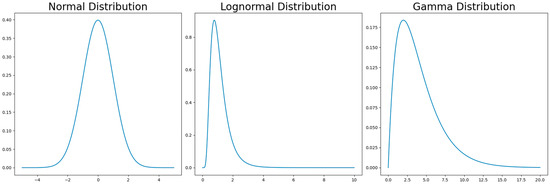
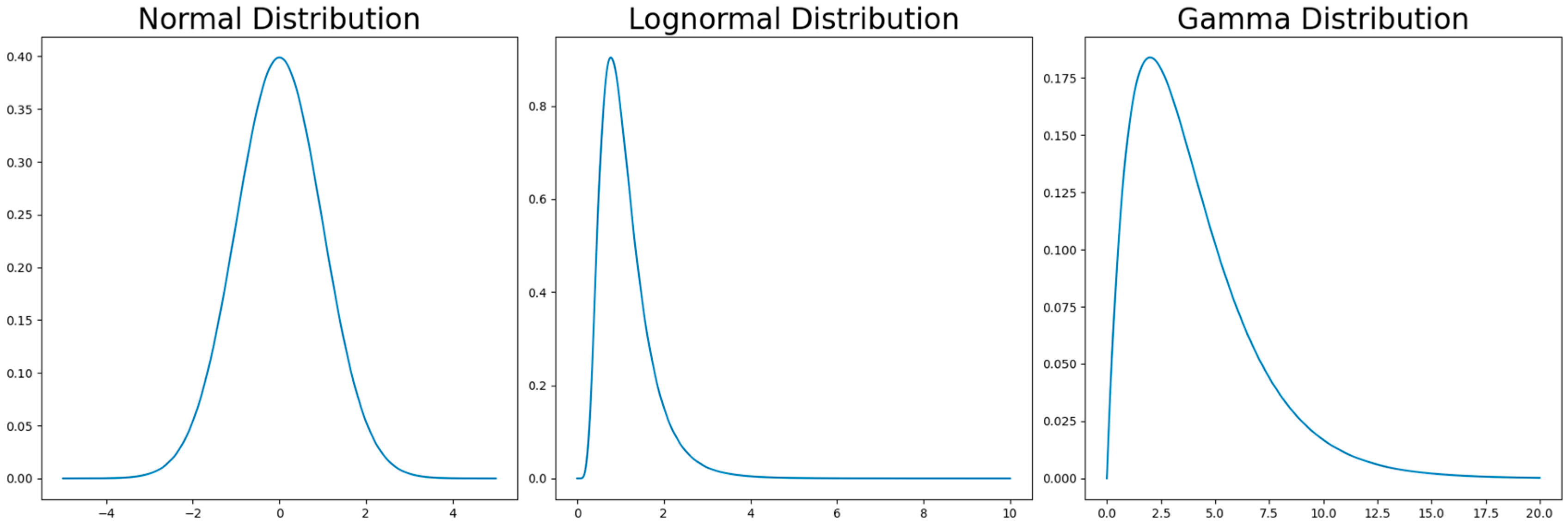
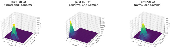
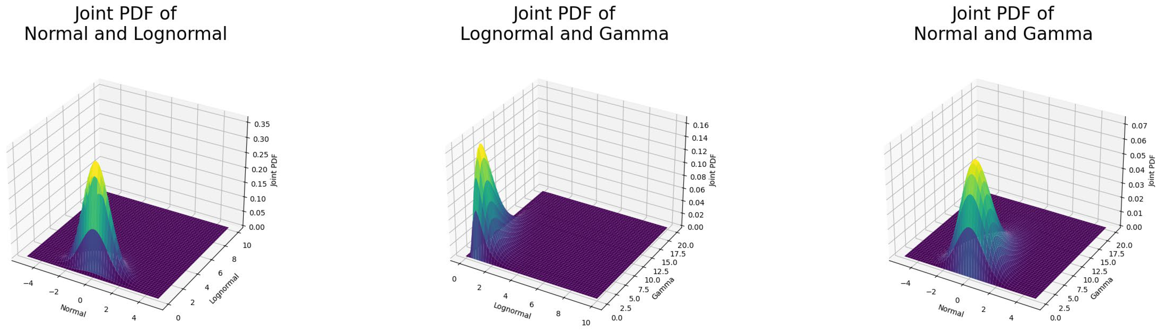
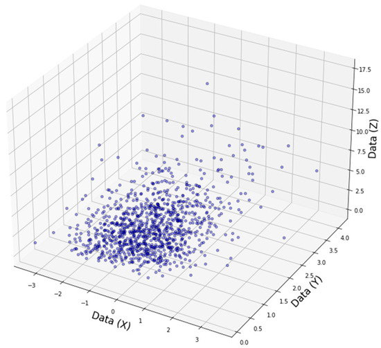
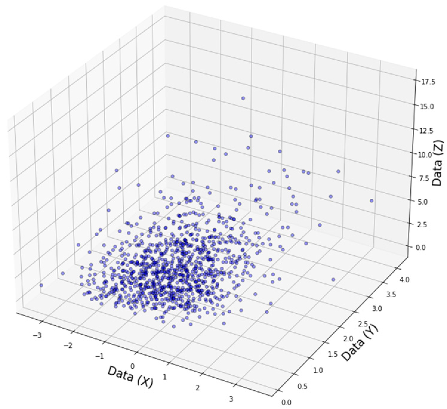
The generated data follows a multivariate normal distribution characterized by a specified mean and covariance matrix (see Figure 1). This ensures that the data captures the intended dependencies among the variables (see pair-wise joint distributions in Figure 2). The joint scatter plot of the three synthesized variables (shown in Figure 3) visually confirms the dependencies imposed by the copula.

Figure 1. Independent graphical representations of the three distributions (normal, lognormal, and gamma) using the set parameter values.

Figure 2. Pair-wise joint PDFs using a 3D surface.

Figure 3. Joint scatter plot of the three synthesized variables.

For that matter, we generate and analyze three various probability distributions (the normal, lognormal, and gamma distributions). In addition, for this current example, we implement the Gaussian copula with the correlation matrix $\left(\mathsf{\Sigma }\right)$ of:

$$\mathsf{\Sigma }=\begin{array}{ccc}1.0& 0.5& 0.3\\ 0.5& 1.0& 0.4\\ 0.3& 0.4& 1.0\end{array}$$

(15)

We begin by defining the parameters for each distribution and subsequently compute their probability density functions (PDFs):

Normal fistribution: Mean $\left(\mu \right)$ of 0 and standard deviation $\left(\sigma \right)$ of 1.

$$f_{\mathrm{Normal}}\left(x\right)={\displaystyle \frac{1}{\mathsf{\sigma }\sqrt{2\mathsf{\pi }}}}\exp \left(-{\displaystyle \frac{{\left(x-\mathsf{\mu }\right)}^2}{2{\mathsf{\sigma }}^2}}\right)$$

(16)

Lognormal distribution: Mean $\left(\mu \right)$ of 0 and standard deviation $(\sigma$) of 0.5.

$$f_{\mathrm{Lognormal}}\left(y\right)={\displaystyle \frac{1}{y\mathsf{\sigma }\sqrt{2\mathsf{\pi }}}}\exp \left(-{\displaystyle \frac{{\left(\ln y-\mathsf{\mu }\right)}^2}{2{\mathsf{\sigma }}^2}}\right)$$

(17)

Gamma distribution: Shape parameter $\left(\kappa \right)$ of 2 and scale parameter $\left(\theta \right)$ of 2.

$$f_{\mathrm{Gamma}}\left(z\right)={\displaystyle \frac{z^{k-1}{e}^{-z/\mathsf{\theta }}}{{\mathsf{\theta }}^k\mathsf{\Gamma }\left(k\right)}}$$

(18)

To examine the joint behavior of pairs of distributions, we create mesh grids for 3D plotting and calculate the joint PDFs for pairs of these distributions under the assumption of independence.

Step 2: Transform the Data to a Uniform Distribution

The next step involves transforming the generated data into a uniform distribution. This is achieved by applying the cumulative distribution function (CDF) of the normal distribution to each value in the generated data. The CDF transformation effectively maps each value to the range between 0 and 1.

By leveraging the properties of the CDF, this transformation ensures that the newly transformed data are uniformly distributed. Despite this, the transformed data retain the dependence structure that was initially imposed by the Gaussian copula.

Step 3: Transform the Uniform Data to the Desired Distributions

The final step involves mapping the uniformly distributed data to the desired marginal distributions: normal, lognormal, and gamma. This is done using the inverse cumulative distribution function (PPF) of each target distribution.

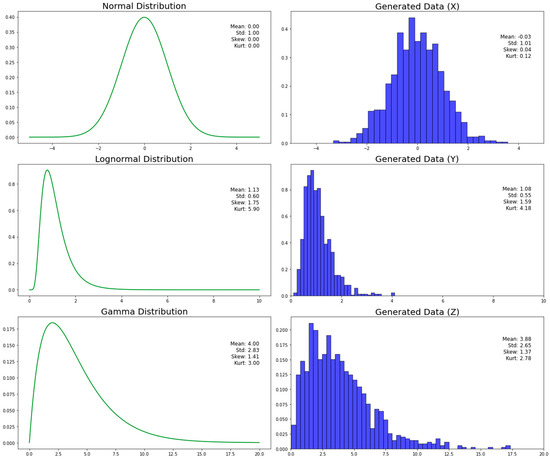
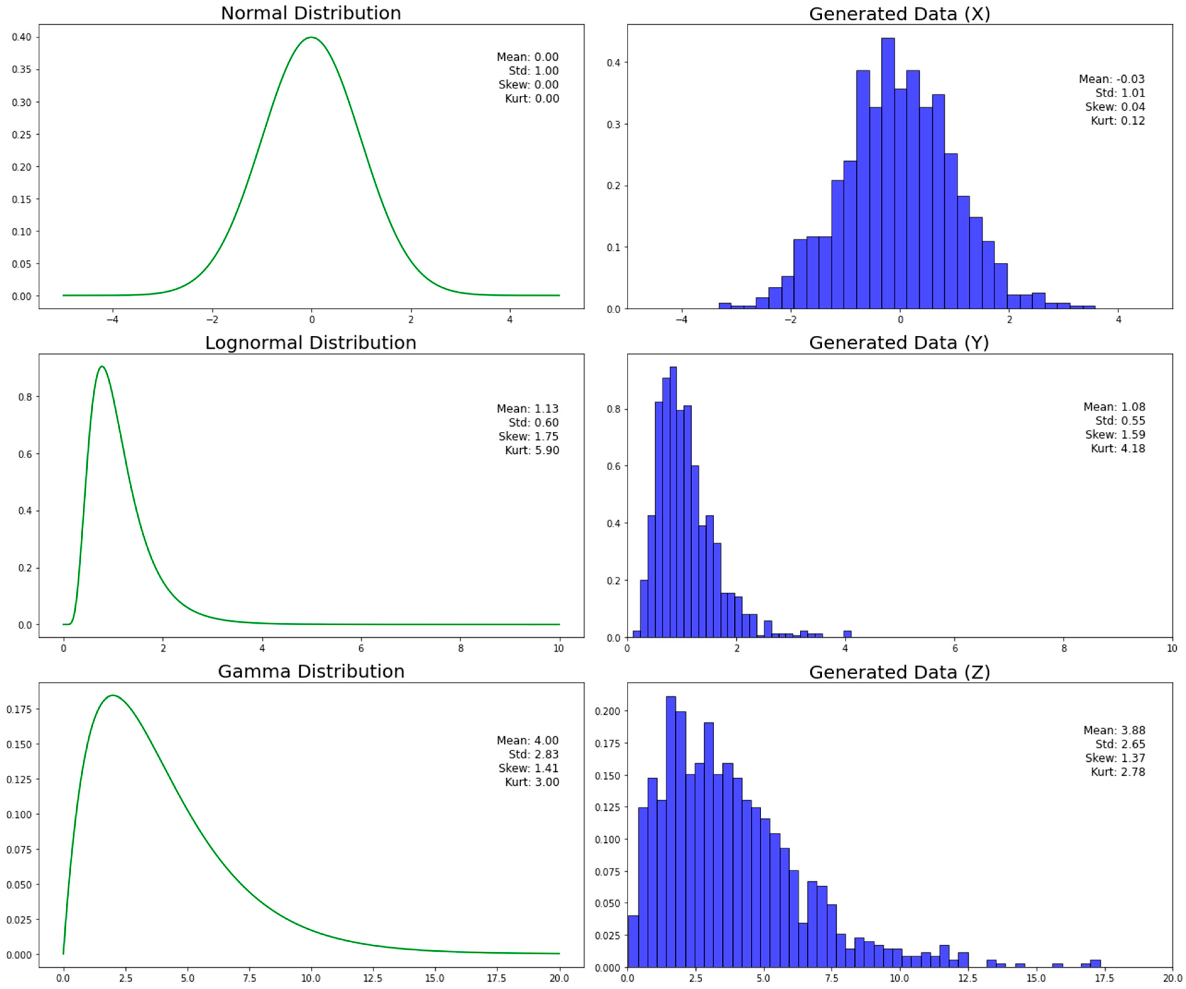
By mapping the transformed data using the respective inverse CDFs, we obtain three generated variables (X, Y, and Z). These datasets now follow the specified marginal distributions while maintaining the dependence structure derived from the original copula. Figure 4 provides a comparison between the resulting empirical distribution parameters and the pre-set theoretical distributions, demonstrating that the synthetic data successfully follows the desired distributions and validates the effectiveness of the copula-based data generation process.

Figure 4. Comparisons of the resulting empirical distribution parameters with the pre-set theoretical distributions.

6. Comparative Evaluation

By comparing the original and synthetic data using the one-sided KS test is used as a comparison vehicle for assessing not only the statistical significance of the copula fit but also the appropriateness of using a given copula family. The five copula families described in the previous sections are tested. The results are shown in Table 1.

Table 1. Resulting Kolmogorov–Smirnov tests for the three variables synthesized by various copula families.

Copula Family	Variable, Set Distribution	One-Sided KS Test, p-Value
Gaussian	X, Normal distribution (μ = 0, σ = 1)	0.006, 0.93
Gaussian	Y, Lognormal distribution (μ = 0, σ = 0.5)	0.003, 0.98
Gaussian	Z. Gamma distribution (κ = 2, θ = 2)	0.012, 0.74
Clayton	X, Normal distribution (μ = 0, σ = 1)	Did not compute *
Clayton	Y, Lognormal distribution (μ = 0, σ = 0.5)	Did not compute *
Clayton	Z. Gamma distribution (κ = 2, θ = 2)	Did not compute *
Gumbel	X, Normal distribution (μ = 0, σ = 1)	Did not compute **
Gumbel	Y, Lognormal distribution (μ = 0, σ = 0.5)	Did not compute **
Gumbel	Z. Gamma distribution (κ = 2, θ = 2)	Did not compute **
Frank	X, Normal distribution (μ = 0, σ = 1)	0.019, 0.49
Frank	Y, Lognormal distribution (μ = 0, σ = 0.5)	0.020, 0.45
Frank	Z. Gamma distribution (κ = 2, θ = 2)	0.034, 0.09
Student	X, Normal distribution (μ = 0, σ = 1)	0.003, 0.15
Student	Y, Lognormal distribution (μ = 0, σ = 0.5)	0.012, 0.75
Student	Z. Gamma distribution (κ = 2, θ = 2)	0.005, 0.95

* The computed theta value −0.069 is out of limits for the given CLAYTON copula. ** The computed theta value 0.968 is out of limits for the given Gumbel copula.

The Gaussian copula showed high fidelity in maintaining the dependencies between features, with minor discrepancies in certain marginal distributions. The one-sided Kolmogorov–Smirnov (KS) tests are conducted to validate the equivalence of the synthetic datasets to their respective theoretical distributions.

In all three cases, the KS tests show high p-values, indicating that the synthetic datasets (X, Y, and Z) are statistically indistinguishable from their respective theoretical distributions. These results validate the effectiveness of our copula-based data synthesis method in preserving the specified dependence structure and producing data that adheres to the desired marginal distributions.

The Clayton copula did not compute a fit. The parameter (theta) computed for the Clayton copula during the fitting process was outside the valid range, as it must be positive because the Clayton copula cannot model negative dependence. If the sample data has negative dependence, the Clayton copula may not be appropriate.

Similarly, the Gumbel copula also did not compute because the fitting parameter was outside the valid range. For the Gumbel copula, the parameter θ must be greater than or equal to one, as it cannot model dependence with θ values less than one. This issue arises when the data used for fitting the copula do not exhibit sufficient dependence for the Gumbel copula, resulting in an invalid θ value.

The results from the KS tests suggest that the synthetic data generated using the Frank copula matches well with the specified theoretical distributions. The high p-values in all three cases indicate that there is no significant evidence to reject the null hypothesis, confirming that the generated synthetic data closely follow the specified distributions. Having said that, all of the results compared to those obtained using the Gaussian copula are worse, indicating that the latter is more suitable for the given set of distributions.

As for the Student’s T copula, the synthetic data also matches well with the specified theoretical distributions. The relatively high p-values in all three cases indicate that there is no significant evidence to reject the null hypothesis, confirming that the generated synthetic data closely follow the specified distributions. Interestingly, the results for the gamma distribution are the best of all tests, inclining that this copula is best suited for the gamma distribution.

7. Conclusions

In this paper, we addressed the challenge of generating synthetic multi-dimensional data that maintains the complex dependencies observed in the original dataset. By leveraging the power of copulas, specifically through the Inverse Copula Sampling method, we demonstrated a robust approach for producing high-quality synthetic data.

Our approach involved three key steps: generating data using various copula families to impose the desired dependence structure, transforming the data to a uniform distribution, and then mapping the uniform data to specific marginal distributions (normal, lognormal, and gamma). The effectiveness of this method was validated through a series of Kolmogorov–Smirnov (KS) tests, which confirmed that the synthetic data closely mimicked the theoretical distributions of the original data.

The experimental results showed high fidelity in maintaining the dependencies between features, with minor discrepancies in certain marginal distributions, as evidenced by the high p-values from the KS tests. These results validate our copula-based data synthesis method as a powerful tool for generating synthetic datasets that preserve intricate interdependencies while adhering to specified marginal distributions.

The Gaussian copula performed the best all-around, meaning that it maintained the pre-set dependencies among the given variables. The KS tests for the Gaussian copula indicated that the synthetic datasets were statistically indistinguishable from their respective theoretical distributions.

The Student’s T copula also produced synthetic data that matched well with the specified theoretical distributions. The relatively high p-values in all three cases indicated that there was no significant evidence to reject the null hypothesis, confirming that the generated synthetic data closely followed the specified distributions. The results for the gamma distribution were particularly noteworthy, suggesting that Student’s T copula is well-suited for the gamma distribution. The results from the KS tests suggest that the synthetic data generated using the Frank copula matched well with the specified theoretical distributions. However, the results were inferior to those obtained using the Gaussian copula, indicating that the Gaussian copula was more suited for the given set of distributions.

The Clayton copula and Gumbel copula did not compute fits as the parameter (theta) computed during the fitting process was outside the valid range. This means that these copula families are not suitable for the pre-set distributions.

The Inverse Copula Sampling method offers a flexible and efficient approach for synthetic data generation, making it an attractive option for various applications in data science, including machine learning model training, simulations, and analytical tasks. Future work could explore the application of other types of copulas and further refine the method to enhance its applicability to an even broader range of data distributions.

References

- Nelsen, R. An Introduction to Copulas, 2nd ed.; Springer: New York, NY, USA, 2006. [Google Scholar]
- Schmidt, T.; Copulas, C.W. Copulas-From Theory to Application in Finance; University of California: Berkeley, CA, USA, 2006. [Google Scholar]
- Mai, J.; Scherer, M. Simulating Copulas: Stochastic Models Sampling Algorithms and Applications. In Copula (Probability Theory)—Infogalactic: The Planetary Knowledge Core; World Scientific: Singapore, 2012. [Google Scholar]
- Mukhopadhyay, S.; Parzen, E. Nonparametric Universal Copula Modeling. arXiv 2019. [Google Scholar] [CrossRef] [Scilit]
- Restrepo, J.P.; Rivera, J.C.; Laniado, H.; Osorio, P.; Becerra, O. Nonparametric Generation of Synthetic Data Using Copulas. Electronics 2023, 12, 1601. [Google Scholar] [CrossRef] [Scilit]
- Benali, F.; Bodénès, D.; Labroche, N.; de Runz, C. MTCopula: Synthetic Complex Data Generation Using Copula. In Proceedings of the International Workshop on Data Warehousing and OLAP, Nicosia, Cyprus, 23 March 2021. [Google Scholar]
- Marchev, A.; Marchev, V. Synthesizing multi-dimensional personal data sets. AIP Conf. Proc. 2022, 2505, 020012. [Google Scholar] [CrossRef] [Scilit]
- Marchev, V.; Marchev, A.; Piryankova, M.; Masarliev, D.; Mitkov, V. Synthesizing an anonymized multidimensional dataset featuring financial, economic, demographic, and personal traits data. Vanguard Sci. Instrum. Manag. 2023, 19, 79–99. [Google Scholar]
- Marchev, V.; Marchev, A. Automated Algorithm for Multi-variate Data Synthesis with Cholesky Decomposition. In Proceedings of the ICACS’23: Proceedings of the 7th International Conference on Algorithms, Computing and Systems, Larissa, Greece, 19–21 October 2023; pp. 1–6. [Google Scholar]
- Sklar, A. Random variables distribution functions and copulas—A personal look backward and forward. Lect. Notes-Monogr. Ser. 1996, 28, 1–14. [Google Scholar] [CrossRef] [Scilit]
- Wan, K.; Kornhauser, A. On the Properties of Gaussian Copula Mixture Models. arXiv 2023. [Google Scholar] [CrossRef] [Scilit]
- Clayton, D. A model for association in bivariate life tables and its application in epidemiological studies of familial tendency in chronic disease incidence. Biometrika 1978, 65, 141–151. [Google Scholar] [CrossRef]
- Kurowicka, D.; van Horssen, W.T. On an interaction function for copulas. J. Multivar. Anal. 2015, 138, 127–142. [Google Scholar] [CrossRef] [Scilit]
- Liebscher, E. Construction of asymmetric multivariate copulas. J. Multivar. Anal. 2008, 99, 2234–2250. [Google Scholar] [CrossRef] [Scilit]
- Manner, H. Estimation and Model Selection of Copulas with an Application to Exchange Rates; RM/07/056; Maastricht Research School of Economics of Technology and Organizations: Maastricht, The Netherlands, 2007. [Google Scholar]
- Fang, R.; Li, X.; Li, L.L. Generalized multivariate Gumbel distributions—Dependence, aging properties and applications. J. Syst. Sci. Complex 2016, 29, 1752–1772. [Google Scholar] [CrossRef] [Scilit]
- Mächler, M. Numerically Stable Frank Copula Functions via Multiprecision: R Package Rmpfr; Technical Report; ETH Zurich: Zurich, Switzerland, 2011. [Google Scholar]
- Lourme, A.; Maurer, F. Testing the Gaussian and Student’s t copulas in a risk management framework. Econ. Model. 2017, 67, 203–214. [Google Scholar] [CrossRef] [Scilit]
- Wilson, A.G.; Ghahramani, Z. Copula Processes. arXiv 2010, arXiv:1006.1350. [Google Scholar]
- Jaworski, P.; Durante, F.; Härdle, W.K.; Rychlik, T. Copula Theory and Its Applications; Lecture Notes in Statistics; Springer: Berlin/Heidelberg, Germany, 2010. [Google Scholar]
- Strelen, J. Tools for Dependent Simulation Input with Copulas. In Proceedings of the 2nd International ICST Conference on Simulation Tools and Techniques, Rome, Italy, 2–6 March 2009. [Google Scholar]
- Massey, F.J., Jr. The Kolmogorov-Smirnov Test for Goodness of Fit. J. Am. Stat. Assoc. 1951, 46, 68–78. [Google Scholar] [CrossRef]
- Drew, J.H.; Glen, A.G.; Leemis, L.M. Computing the cumulative distribution function of the Kolmogorov–Smirnov statistic. Comput. Stat. Data Anal. 2000, 34, 1–15. [Google Scholar] [CrossRef] [Scilit]
Disclaimer/Publisher’s Note: The statements, opinions and data contained in all publications are solely those of the individual author(s) and contributor(s) and not of MDPI and/or the editor(s). MDPI and/or the editor(s) disclaim responsibility for any injury to people or property resulting from any ideas, methods, instructions or products referred to in the content. |
© 2026 by the authors. Licensee MDPI, Basel, Switzerland. This article is an open access article distributed under the terms and conditions of the Creative Commons Attribution (CC BY) license.