


Abstract
Equipping municipal service vehicles with GPS and activity sensors and displaying this data on an interactive map is the first step towards creating a “smart city” infrastructure to improve planning and provide proof of service. Without a proper link between the data and the map, a human operator must evaluate whether the vehicles are performing their designated tasks by estimating their actual routes. In this paper, we develop a map-matching algorithm that maps the location data from the GPS sensors on such vehicles to the respective street segments in a GIS setting, removing the need for human operator evaluation.
1. Introduction
Effective control over cleaning activities is an important part of ensuring that cities stay clean and provide a pleasant urban environment. In the city of Sofia, the Sofia Municipality delegates those activities to contractor firms, and the Inspectorate of the Sofia Municipality issues orders and supervises the cleaning operations carried out by the firms. Operational plans determine the desired level of service, and sensors in the municipal service vehicles provide information about what activities were performed. The Inspectorate uses an information system that presents this information to inspectors who validate if the contractors have performed the planned activities.
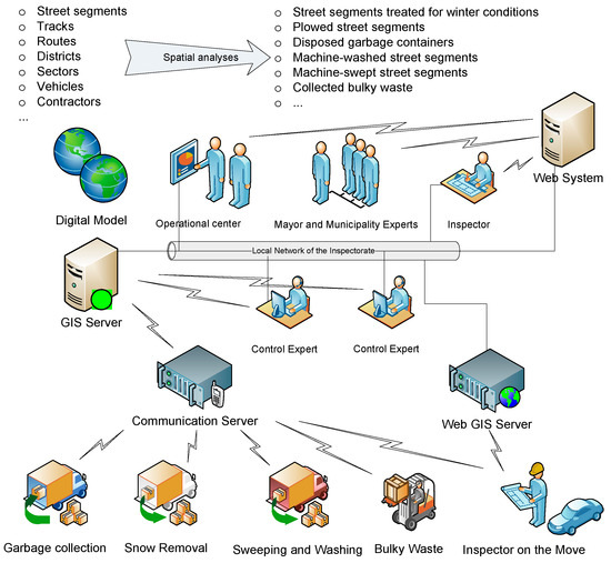
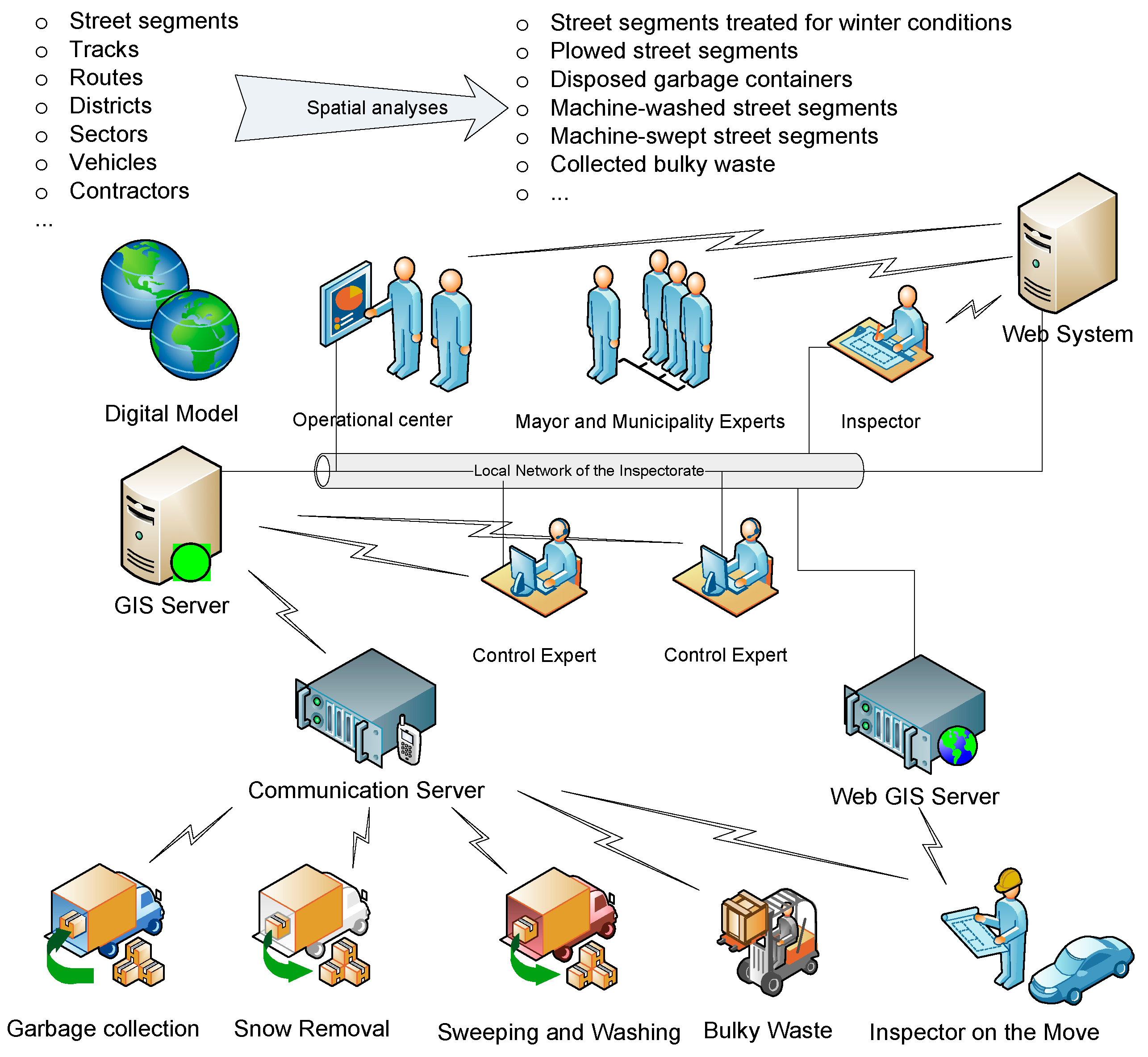
The system architecture (Figure 1) illustrates the main components of the system.
Figure 1.
System architecture of municipal service vehicle management.
- All service vehicles and the vehicles of the inspectors are equipped with GPS tracking modules. For municipal service vehicles, those modules are also connected to sensors in the vehicle, depending on the vehicle equipment type—sensors for plowing and spreading for snow removal vehicles, sensors for activating the shooter for garbage collection vehicles, and so on.
- A communication server receives, stores and processes the data from the vehicles.
- A GIS server augments the raw data with additional spatial and non-spatial information, such as street segments, districts, sectors, and more. The GIS server is at the core of the digital model that, using spatial analysis algorithms, can answer questions such as which street segments were treated for winter conditions, which garbage containers were disposed of, which street segments were washed or swept, and so on.
- A web GIS server enables access to the digital model for inspectors on the move.
- A web system is the final software component of the system architecture. The web system is integrated with the rest of the components and provides a convenient user interface for the inspectors, the people in the operational center, the mayor and the municipality experts to view and analyze the information in the system.
Overall, the operational center, control experts, and inspectors collaborate using digital models and GIS data to ensure efficient municipal service management.
A major aspect of this management is the control function of the inspectorate over the contractors. The inspectors have to verify that the contractors are performing according to the operational plans. For winter activities, sweeping and washing, this comes down to verifying that the respective activities were performed on specific street segments.
The traditional approach of manually matching GPS location data from service vehicles to street segments is time-consuming and prone to errors. To address these challenges, a map-matching algorithm was developed to provide an automated solution, offering significant improvements in accuracy and efficiency.
2. Data Sources
In order to perform map matching, it is necessary to have a proper map that contains the roads for matching. Two sources of road data were evaluated: Open Street Map (OSM) and the linear layer of “GIS Sofia”—the municipality-owned company that develops, updates and manages the information system for the cadastral, regulational and building plans for the Sofia Municipality.
The linear layer of OSM was found to have good coverage of the streets in Sofia. However, there were some topological issues, such as a single street segment being represented as multiple polylines and a lack of information about the starting and ending levels of the street segments, which made it difficult to handle bridges and underpasses.
In contrast, the linear layer of “GIS Sofia” had perfect topological consistency: street segments were single polylines, all intersecting streets had intersecting street segments, and bridges and underpasses did not cross with segments on another level. Therefore, the linear layer from “GIS Sofia” was used as the street model. This model was augmented with information from the inspectorate, such as street segments for mass transit, streets of public importance and dangerous or steep segments.
The other major source of data is the information reported from sensors on the vehicles of the contractor companies of the Sofia Municipality. The contractor companies are obliged to send this data to the inspectorate. One data point contains:
- The GPS time of the event;
- The GPS location (latitude and longitude);
- The speed of the vehicle;
- The state of the sensors in the vehicle.
One important aspect to consider is the sampling rate for the vehicle data. Typically, the sampling rate is high—once every 5 s. However, given that there are hundreds of vehicles operating in city conditions, often with buildings obscuring the GPS satellites, there is significant variability in the actual sampling rate, sometimes going as low as one data point every 2 min.
3. Approach to Map Matching
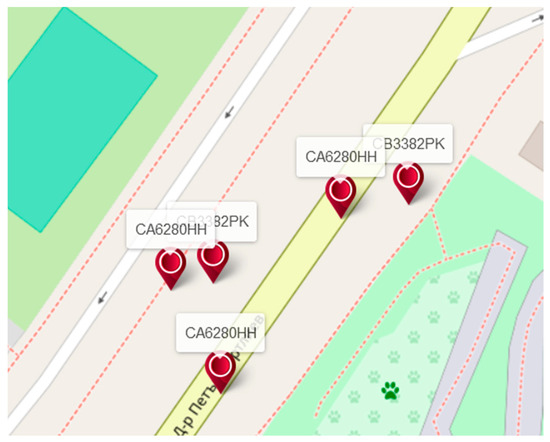
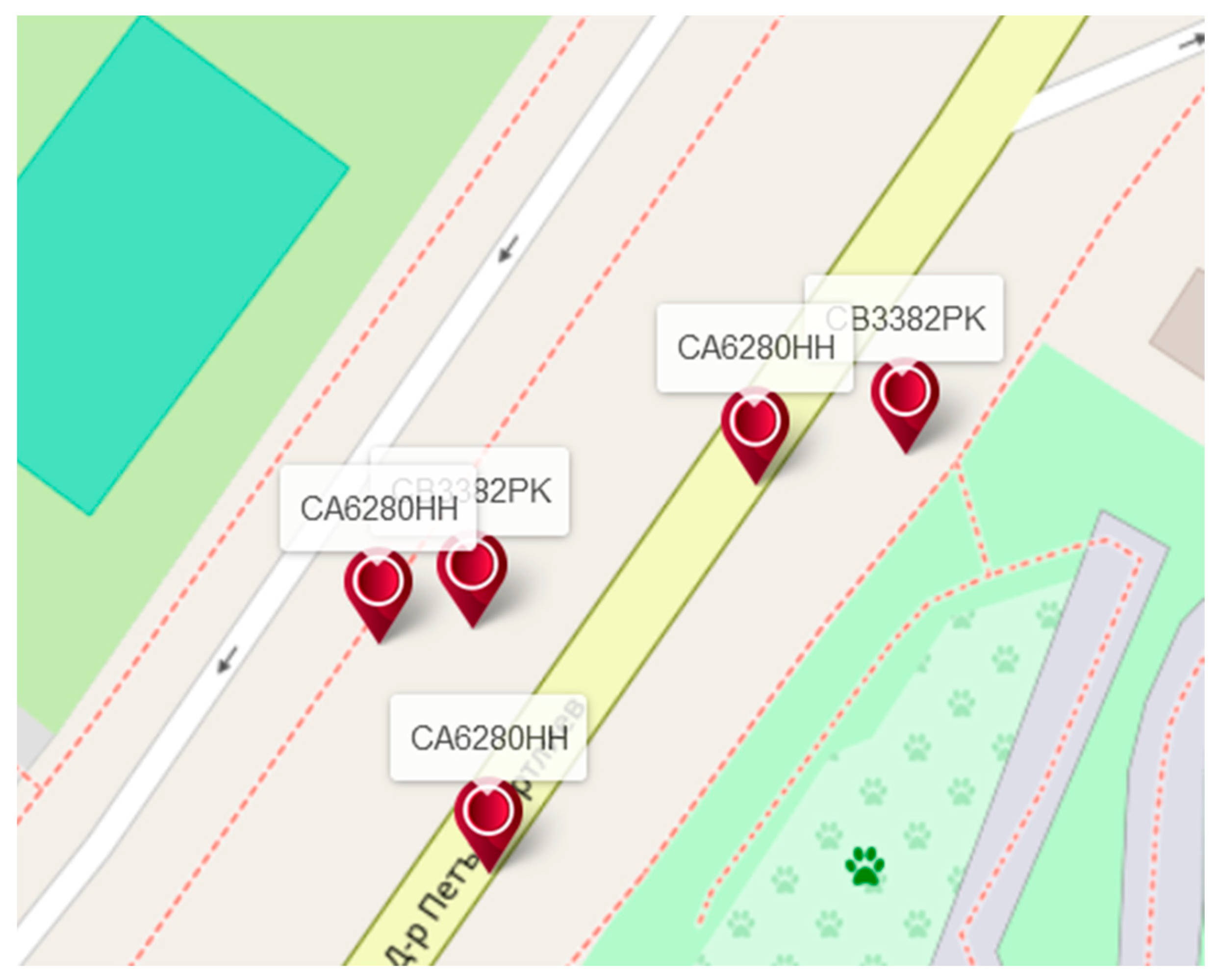
The major issue when trying to verify whether a specific activity was performed on a street segment is determining if a vehicle performed the activity on the street segment within a specific timeframe. An inspector looking at the raw data from the vehicles will see a report similar to the one shown in Figure 2.
Figure 2.
A raw report of vehicle location data. The text above each pin is the vehicle’s license plate number.
In this report, the users have to guess or estimate the actual route taken by the vehicles based on a set of points which, due to the inherent error of GPS measurements, is often several meters away from the actual positions of the vehicles.
The process of aligning a sequence of observed positions with the road network on a digital map is called “map matching”. Our approach to map matching builds on an algorithm called ST-matching, designed for data with a low sampling rate [1].
In our case the data has a variable sampling rate, sometimes high and sometimes low. Preliminary testing shows that the ST-matching algorithm performs well in both cases, which makes it a good match. Also, the algorithm is relatively easy to implement using the data structures available in Acstre GIS 2.3, the GIS software we use in this system.
3.1. Characteristics of the ST-Matching Algorithm
The ST-matching algorithm is a global map-matching algorithm, i.e., it considers the entire trajectory to find the most likely match. The algorithm makes two assumptions:
- True paths tend to be direct rather than roundabout.
- True paths tend to follow the speed constraints of the road.
Based on these assumptions, the authors developed a map-matching algorithm that uses two components to evaluate the candidate paths: a spatial component that accounts for the geometrical and topological information available, and a temporal component that accounts for the information regarding the speed of the roads and the vehicles.
The algorithm, in a nutshell, is as follows:
- For each point of the observed path , retrieve a set of candidate points on the nearby edges of the road graph. This is the candidate preparation step.
- For each candidate, evaluate a spatio-temporal function that signifies the likelihood that the observed point lies on the candidate point.
- Construct the path by traversing the sequence of candidates with the highest sum of the spatio-temporal function across all candidates for all observed points, and join the candidates by finding the shortest path between them.
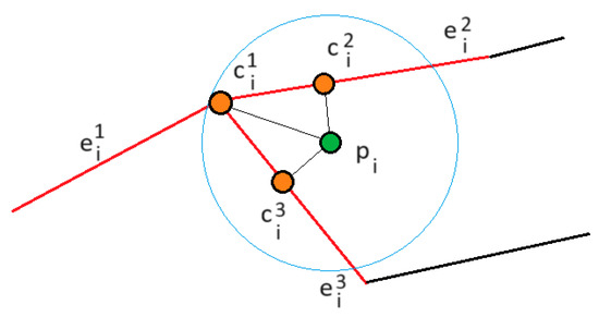
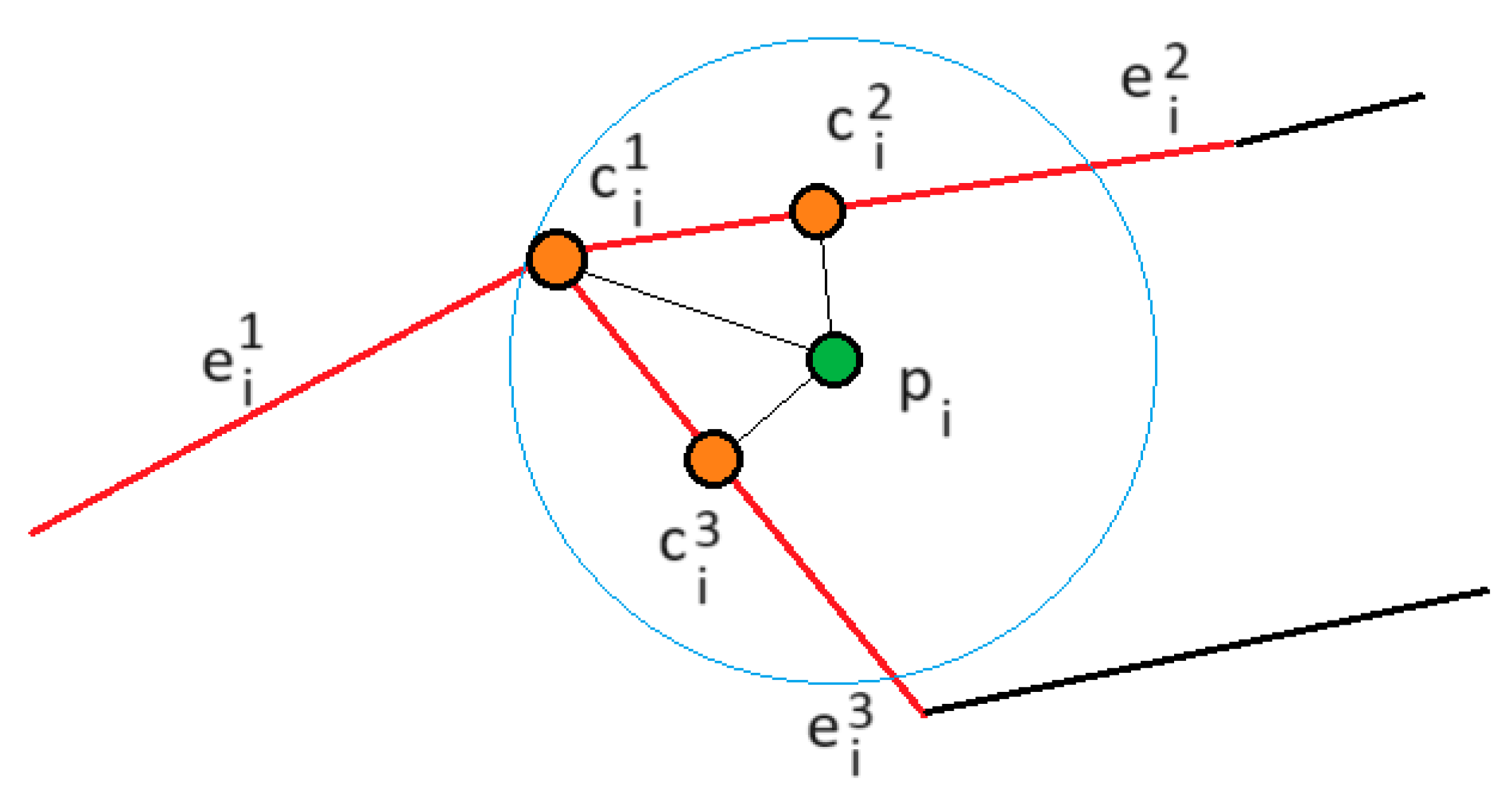
The essence of the candidate preparation step in the ST-matching algorithm is shown in Figure 3.
Figure 3.
The candidate preparation step of the ST-matching algorithm. The observed point is and the blue circle is the maximum search distance. The red edges are street segments that have candidate points within the search distance.
The spatio-temporal function in the ST-matching algorithm is actually the product of three separate functions: the observational probability, the transmission probability and the temporal analysis function.
The observational probability expresses the geometric information shown in Figure 3. It is defined as the zero-mean normal distribution of the distance between a point and a candidate with a standard deviation of 20 m.
The transmission probability is the likelihood that the path between two points follows the shortest path between them.
The temporal analysis function in the ST-matching algorithm is defined as the cosine similarity between the actual average speed between candidates and the speed constraints of the path.
The final spatio-temporal function in the ST-matching algorithm is the product of these three functions.
Now, let’s validate the assumptions of the ST-matching algorithm. Firstly, do true paths tend to be direct rather than roundabout for municipal service vehicles? For a normal vehicle, the purpose of travel is usually to get to the destination. There may be several destinations to get to, for example “go home but visit the grocery store and the drug store on the way”. Google Maps, for example, would only allow for up to 9 destinations besides the starting point when calculating a route [2]. But for a municipal service vehicle, there may be hundreds of destinations (all the garbage containers to collect) or the purpose of the vehicle is to cover a large part of the road network (for example, to plow the snow or to wash the streets). So, globally, this assumption is not true for municipal service vehicles. However, it is true locally, when going between (nearby) destinations. Thus, at a high enough sampling rate, respective to the time it takes for the vehicle to perform an activity, this assumption is true. In our case, the typical sampling rate is high enough, and even when it gets low, the activities themselves tend to take a significant amount of time relative to it—disposing a single garbage container would often take in the order of one minute, and the vehicles need to move slowly for effective sweeping, washing and snowplowing.
The last point is crucial when evaluating the second assumption of the algorithm. True paths tend to follow the speed constraints of the road for vehicles that can move at speeds higher than the speed constraints of the road. This is not true for municipal service vehicles. These vehicles will move slowly every time they perform their designated activities, regardless of if they are on city highways, high-speed boulevards, service roads or internal streets. Therefore, the temporal aspect of the ST-matching algorithm has to be adapted to the specifics of service vehicles.
3.2. Map-Matching Algorithm Inputs and Outputs
3.2.1. Inputs
While the temporal component of the ST-matching algorithm is not directly applicable in our case, it does provide valuable insight: additional temporal information can improve the outcomes of a map-matching algorithm. The speed of a vehicle, in particular, can make certain paths unlikely or impossible. This information is available when using a GPS tracking device. Therefore, we included it as input into the map-matching algorithm. Specifically, we used the following inputs:
- Point data: x, y, GPS speed, and GPS time.
- Standard deviation of the normal distribution of the distance between a point and a candidate, (typically 20).
- Maximum search distance (typically ).
- Road data: a set of polylines and a set of nodes where polylines connect.
The point data was the ordered set of points that was received from the vehicle’s GPS tracker. We included the standard deviation σ and the maximum search distance because we retained the same candidate preparation step as the ST-matching algorithm.
The road data is available to the algorithm in the native way that Acstre GIS stores it. In Acstre GIS, there is a special point object called a node. Nodes are maintained automatically as polylines are created, modified and deleted. They are the points where polylines begin or end. Each polyline in Acstre GIS keeps the IDs of the nodes at its first and last points. Each node keeps a list of the IDs of the polylines that connect to it—many polylines can start or end in the same node. This structure allows for a very efficient connected polyline traversal, which is important for many algorithms, including pathfinding.
3.2.2. Outputs
In an ideal scenario, the model of the road network is complete and there are no missing or erroneous street segments or missing connections between street segments. Also, vehicles only travel on the roads that exist. In the real world, there may be missing road connections in the model due to errors, recent construction of new roads or the construction of temporary roads, and drivers may occasionally drive vehicles outside the road network. It is desirable that the map-matching algorithm can handle such cases gracefully, by matching as much of the route to streets as physically possible. Therefore, the result of the map-matching algorithm for a single input path is a list of routes, not a single route. Also, because some points may not match to the road network at all, the output includes a list of the indices of all points that were not matched to a route during the execution of the algorithm. For each route, we construct a list of visited polylines, where, for each visited polyline, we return:
- ID of the polyline.
- Enter Time—when the vehicle entered the polyline.
- Exit Time—when the vehicle exited the polyline.
- Enter Point—coordinates and the indices of the neighboring points of the polyline.
- Exit Point—coordinates and the indices of the neighboring points of the polyline.
This information is sufficient to fully reconstruct the routes through the street segments of the road model and also handles cases where the routes do not start or end at the beginning or end of a street segment, so a partial service of a street segment can be detected and reported.
4. Map-Matching Algorithm for Municipal Service Vehicles
4.1. Proposed Algorithm
Taking the above into account, we propose the following map-matching algorithm for municipal service vehicles:
- For each point , find a set of candidates within the maximum search distance and for each:
- o
- Calculate and store
- o
- If this is the first point, or if there is no parent candidate with non-zero probability, make the path probability the observational probability.
- o
- If this is not the first point, calculate the transmission probability from each previous candidate to this one:
- ▪
- Calculate the maximum permissible path length between and .
- ▪
- Calculate the shortest path until either the maximum permissible path length has been reached or the shortest path has been found.
- ▪
- If a path was found, store , or else set the transmission probability to zero.
- ▪
- If this is the best path probability so far, store it as “best” for the candidate.
- Construct the best route by tracing back to the best candidates from the highest sum of probabilities in the final set of candidates, and add them to the list of routes. For points with no parent candidate and no polylines in their routes, add them to the list of not mapped points.
In the algorithm above, the highlighted parts are where the algorithm behaves differently from the ST-matching algorithm.
Firstly, we return a list of routes instead of single route; therefore, there could be several “first” points—points that start a new route. We make the path probability for those candidates the observational probability, like the first point in the ST-matching algorithm.
Then, we observe that it is highly inefficient to calculate the actual length of all the shortest paths between the candidates of neighboring observations. When the observed points lie between two parallel roads, there will be many transmissions between candidates lying on different roads. If the roads do not have intersections nearby, the shortest paths between them could be very long—we have observed lengths of over one kilometer. It would be physically impossible for a vehicle to travel that long in just a few seconds, especially if it is a slow-moving service vehicle. Therefore, we use the temporal information available in the GPS tracker to calculate a maximum permissible length of the path between two candidates. We then use a modified pathfinding algorithm to stop the path search as soon as the length exceeds the maximum permissible length.
In our algorithm, if the pathfinding algorithm does not find a short enough path, we set the transmission probability to zero.
As we construct the best route, we can find zero probability transmissions. This is where we split the results into multiple routes. Thus, setting a limit on the maximum length of a path is not just performance optimization—when a road connection is missing from the model or the driver has crossed between roads that are not connected, impossibly long paths are returned by the standard ST-matching algorithm in the final result. In out algorithm, they are not—we split the route instead.
Finally, we add observed points that were not part of any route to the list of not mapped points.
4.2. Calculating the Maximum Permissible Path Length
To calculate the maximum permissible path length between two observed points, and , we use the following inputs:
- —the GPS speed of the vehicle at .
- —the GPS time at which the vehicle was at .
- —the GPS speed of the vehicle at .
- —the GPS time at which the vehicle was at .
- Safety margin—a constant that ensures a minimum speed is used in the calculation.
- Maximum Speed—a constant used in the absence of GPS speed information.
The idea behind the algorithm is to calculate a maximum average speed that the vehicle may have reached between the two points, and then calculate the length of the path based on this speed and the time it took to get from the first point to the second. The result of the algorithm is the maximum path length. Note that this is not designed to be an estimate of the actual length of the path; rather, it is an upper bound—we need to ensure that no valid paths are longer than the calculated result. Therefore, to account for GPS inaccuracies, we have introduced a safety margin—a constant that is added to the calculated speed from the GPS data. We have found empirically that 10 m/s (36 km/h) is enough to offset this effect. In the absence of GPS speed data, we use a fallback of 150 km/h, which is a defensive value, well above the speed limits in the city.
More formally, we use the following algorithm:
- Set to
- If either or are set:
- o
- ,
4.3. Finding the Shortest Path Between Two Points
This is a classical problem that has been the subject of extensive research [3]. We use a modified version of the A* algorithm, where the algorithm performs an early return if the length of the path so far exceeds the maximum permissible path length. We use Euclidean distance as the heuristic in the A* algorithm.
5. Results
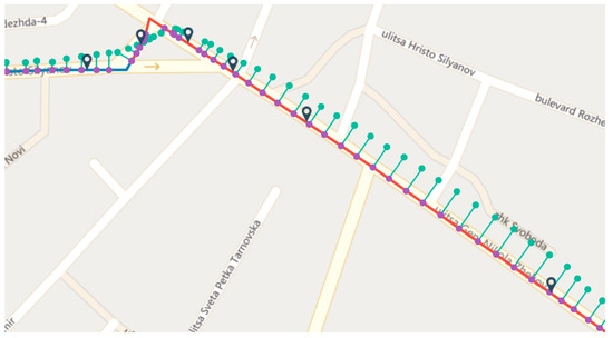
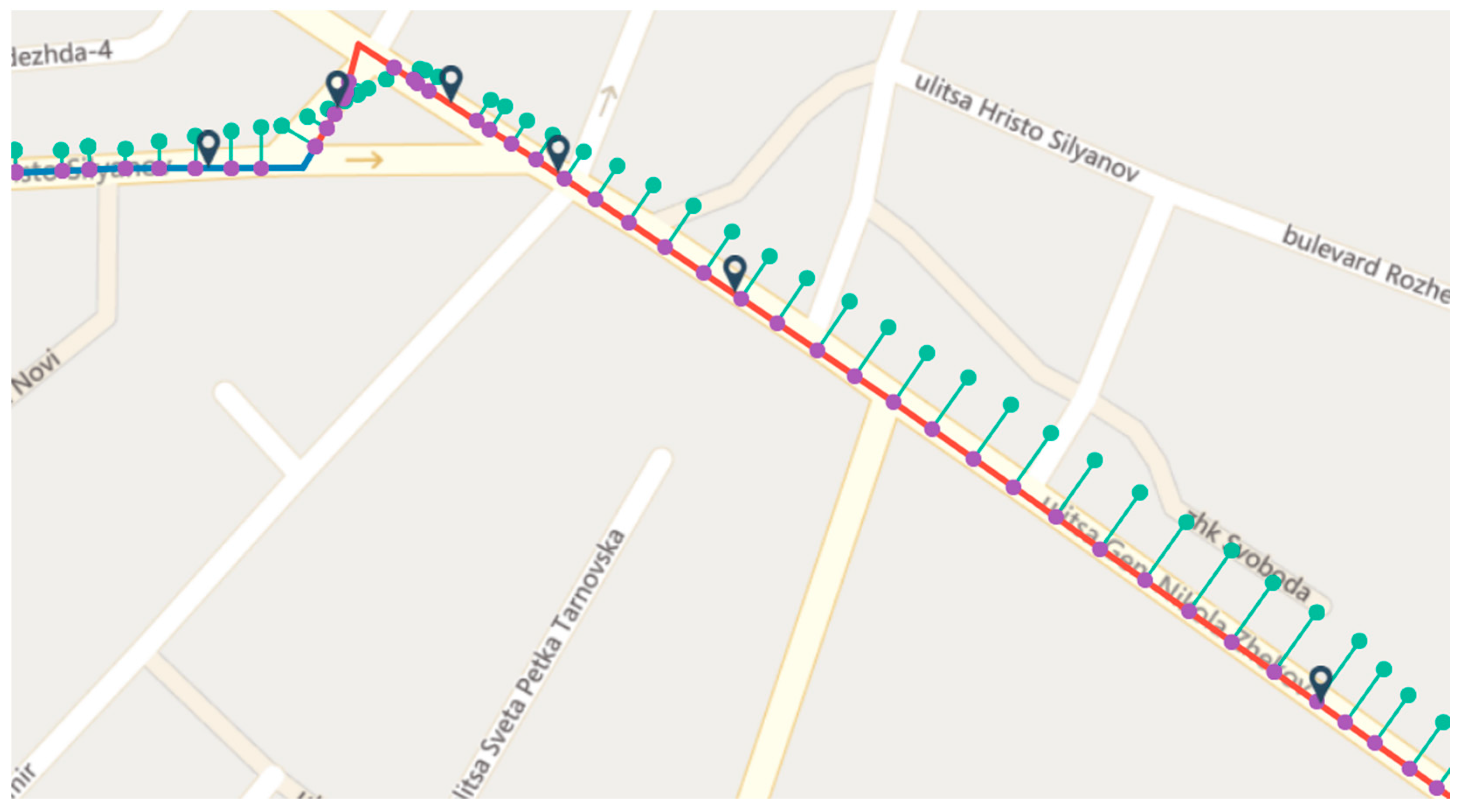
We have used the proposed algorithm to successfully perform map matching of GPS tracks from municipal service vehicles to street segments. A sample match is shown in Figure 4.
Figure 4.
A map-matched route using the proposed algorithm. The teal dots represent observed points. The purple dots represent the selected best candidates. The red and blue lines are the matched street segments (the color depends on the active sensors). The dark pins are placed in the middle of each street segment.
6. Future Work
In the future, additional data from the vehicles may be used to further reduce human work. In recent years we have seen increased usage of automated systems to replace human labor. For example, for garbage collection, a driver with one or two helpers is replaced with a one-man operated, bilateral lifting system for the collection of recyclable waste [4]. It is foreseeable that in the future, unmanned municipal service vehicles may remove human operators entirely. Promising improvements in autonomous logistics are suggested by [5] for computer vision problems in monocular video by applying a heat map approach providing real-time operation.
7. Conclusions
The map-matching algorithm proposed in this paper is a modification of the ST-matching algorithm, which is more suitable for slow-moving vehicles, such as municipal service vehicles. The algorithm has the following key improvements over ST-matching for such vehicles:
- ST-matching considers the average speed of the road; the proposed algorithm removes this bias to better suit low- and constant-speed vehicles.
- The proposed algorithm sets a hard limit on the maximum distance traveled between two points based on vehicle speed, which improves performance.
- The proposed algorithm allows the route to split based on topological or temporal data and thus handles missing or malformed road segments.
Funding
The publishing of this article was funded by the Research and Development Sector at the Technical University of Sofia.
Institutional Review Board Statement
Not applicable.
Informed Consent Statement
Not applicable.
Data Availability Statement
The datasets presented in this article are not readily available because they belong to the Sofia Inspectorate. Requests to access the datasets should be directed to the Sofia Inspectorate.
Acknowledgments
The author would like to thank the Research and Development Sector at the Technical University of Sofia for their financial support.
Conflicts of Interest
The author declares no conflict of interest.
Abbreviations
The following abbreviations are used in this manuscript:
| GPS | Global Positioning System |
| GIS | Geographic Information System |
| OSM | OpenStreetMap |
| ST | Spatio-Temporal |
References
- Lou, Y.; Zhang, C.; Zheng, Y.; Xie, X.; Wang, W.; Huang, Y. Map-matching for low-sampling-rate GPS trajectories. In Proceedings of the 17th ACM SIGSPATIAL International Conference on Advances in Geographic Information Systems (GIS ’09), Seattle, WA, USA, 4–6 November 2009. [Google Scholar] [CrossRef] [Scilit]
- Google. Get Directions & Show Routes. 2024. Available online: https://support.google.com/maps/answer/144339?hl=en&co=GENIE.Platform%3DDesktop (accessed on 5 June 2024).
- Foead, D.; Ghifari, A.; Kusuma, M.B.; Hanafiah, N.; Gunawan, E. A Systematic Literature Review of A* Pathfinding. Procedia Comput. Sci. 2021, 179, 507–514. [Google Scholar] [CrossRef] [Scilit]
- NORD Engineering. Wase Colleciton, Made Easy. 2024. Available online: https://www.nordengineering.com/en/ (accessed on 10 June 2024).
- Marinov, P. Improving autonomous logistics by optimizing the recognition in real time of moving objects. In Proceedings XXII ISCME’24, Sozopol, Bulgaria; Springer Nature: Cham, Switzerland, 2024. [Google Scholar]
Disclaimer/Publisher’s Note: The statements, opinions and data contained in all publications are solely those of the individual author(s) and contributor(s) and not of MDPI and/or the editor(s). MDPI and/or the editor(s) disclaim responsibility for any injury to people or property resulting from any ideas, methods, instructions or products referred to in the content. |
© 2026 by the author. Licensee MDPI, Basel, Switzerland. This article is an open access article distributed under the terms and conditions of the Creative Commons Attribution (CC BY) license.