Physics-Informed Operating Region Design of Dual Active Bridge Converters Under Thermal and ZVS Constraints for Spacecraft Electrical Power Systems ^†

Abstract

The dual active bridge (DAB) converter is one of the most common types of isolated bidirectional power converters in modern spacecraft EPS owing to its galvanic isolation, bidirectionality, soft switching, and good controllability. However, the goal of power transfer maximization often clashes with real-world spacecraft EPS constraints, namely thermal compliance, reliability, and the accuracy of simplified models used for analysis. This paper proposes a physics-informed methodology to derive the practical operating range under single phase shift (SPS) control based on a rigorous piecewise time-domain representation. From this model, the steady-state initial condition, general closed-form RMS current expression, ZVS boundary condition, and ZVS-aware loss model linked to the junction-temperature estimate are derived. The validity domain of the fundamental harmonic approximation (FHA) is evaluated against the exact model across the full (φ, k) space, and a two-dimensional operating map superposing power contours, the ZVS limit, and the thermal limit is presented. For the baseline case study at k = 1.0, the thermal constraint limits the nominal feasible upper phase shift to approximately 35°, while the broader 15–45° range remains useful for design assessment and operation toward 45° requires lower effective resistance and/or improved thermal management. The normalized SPS power-transfer curve retains the same shape under variations in L and f_s, but RMS current, losses, and thermal feasibility must be reassessed for each converter design. The resulting closed-form framework provides a steady-state feasibility-evaluation tool for spacecraft EPS design and offers a computational basis for future supervisory constraint evaluation under varying voltage, load, and thermal conditions.

1. Introduction

Spacecraft electrical power systems require DC–DC converters that combine galvanic isolation, bidirectional energy flow, high power density, and well-characterized thermal behavior across a wide range of bus voltage conditions [1,2,3]. The dual active bridge (DAB) converter, introduced by De Doncker, Divan and Kheraluwala [4,5], is a prime candidate, possessing symmetrical H-bridge configuration that permits soft switching as well as power flow reversal by changing the sign of the phase shift.

Despite its topological advantages, the DAB converter presents a non-trivial design challenge in the spacecraft context. The standard single phase shift (SPS) modulation strategy produces a power transfer characteristic that peaks at φ = 90° [4,5]. However, operation near maximum power causes a sharp increase in the inductor RMS current, associated with elevated conduction and switching losses [6,7], and—critically—junction temperatures that may violate device ratings under the passive thermal management typical of spacecraft [1,3].

Another difficulty is that while the FHA is a common approach for analysis and control [8,9], its accuracy decreases as the phase shift increases [8,10]. This model error grows significantly at large phase shifts, precisely where the thermal stress is highest.

A further constraint is the zero-voltage switching (ZVS) condition—required for soft switching of all eight devices—which imposes a minimum phase shift that rises as the voltage ratio deviates from unity [11,12].

These three constraints—thermal compliance, ZVS, and FHA model validity—have been studied individually [6,7,10,11,12,13], but their simultaneous imposition on a unified operating region for spacecraft EPS remains insufficiently integrated.

This study addresses this gap by developing a physics-informed operating region framework that integrates the power-transfer behavior, RMS current stress, switching conditions, and thermal constraints.

The main contributions of this study are as follows: (i) an exact closed-form RMS expression validated against a numerical time-domain simulation with an error below 1.3%; (ii) quantitative FHA error characterization over the full (φ, k) operating space; (iii) a ZVS-aware loss and thermal model; (iv) a generalized 2D operating map; and (v) spacecraft operating region synthesis with practical design recommendations. Table 1 compares the proposed framework against several representative prior contributions.

Table 1. Compares the proposed work against several relevant prior contributions. Bold indicates the framework proposed in this work.

Reference	Exact Irms	FHA Error	ZVS Bdry	Thermal	V-Ratio	S/C EPS	Unified Map
De Doncker [4]	Partial	No	No	No	No	No	No
Kheraluwala [5]	Partial	No	Yes	No	No	No	No
Bai & Mi [10]	No	Partial	No	No	No	No	Partial
Oggier [12]	No	No	Yes	No	No	No	Partial
Krismer [6]	Yes	No	Yes	Yes	No	No	No
Naayagi [1]	Partial	No	Partial	No	Partial	Yes	No
Proposed	Yes	Yes	Yes	Yes	Yes	Yes	Yes

2. DAB Converter Operating Principle

The DAB converter consists of two full H-bridges connected through a high-frequency transformer with series inductance L. Under SPS modulation, the primary bridge generates v₁(t) at amplitude V₁ and the secondary bridge generates a phase-shifted v₂(t) at amplitude V₂. The transformer turns ratio n = N₁/N₂ refers all quantities to the primary side; referred secondary voltage V₂ᵣ = nV₂. Power flows from the primary to the secondary when φ > 0 and reverses when φ < 0, making the DAB intrinsically bidirectional [4,5].

For the representative spacecraft EPS case study considered in this work, V₁ = 100 V (high-voltage source bus), V₂ = 28 V (regulated distribution bus), n = 100/28 ≈ 3.571 (V₂ᵣ = 100 V, k = 1.0, nominal), L = 20 μH, f_s = 50 kHz, and R_eq = 50 mΩ. These values are baseline converter-design parameters adopted for the present case study, while the use of the DAB topology for aerospace bidirectional power conversion is supported by [1,2].

To assess sensitivity to bus-voltage variation, the voltage ratio $k={\displaystyle \frac{V_2ᵣ}{V_1}}$ was wide-ranging over k ∈ [0.70,1.30], selected in this study as a broad parametric range around the nominal operating point k = 1.0.

The inductor ODE is

$$L{\displaystyle \frac{d{i}_L}{dt}}+R_{eq}{i}_L=v_L(t)$$

where

$$v_L\left(t\right)=v_1\left(t\right)-v_{2r}\left(t\right)$$

The piecewise solution of this equation forms the basis for time-domain analysis.

Under SPS operation, and in particular for φ ∈ (0°, 90°), the switching cycle consists of four segments determined by the switching instants of the primary and secondary bridges. ${\phi }_t$ is defined as the phase-shift time delay, expressed as ${\displaystyle \frac{\phi }{360f_s}}$, and $T_s=1/f_s$. The states of the bridges, as well as the voltage across the inductor in each of the four segments, are presented in Table 2.

Table 2. SPS switching segments and the inductor voltage.

Segment	Interval	v1(t)	v2ᵣ(t)	vL(t) = v1 − v2ᵣ
0	0 → ${\phi }_t$	+V1	−V2ᵣ	V1 + V2ᵣ
1	${\phi }_t$ → $T_{s/2}$	+V1	+V2ᵣ	V1 − V2ᵣ
2	$T_{s/2}$ → $T_{s/2}$ + ${\phi }_t$	−V1	+V2ᵣ	−(V1 + V2ᵣ)
3	$T_{s/2}$ + ${\phi }_t$→ $T_s$	−V1	−V2ᵣ	−(V1 − V2ᵣ)

The net volt-second integral of the inductor over a complete switching cycle is guaranteed to be zero for any phase shift value, which shows that the inductor voltage experiences no DC bias under steady state SPS modulation [4,5].

3. Analytical Models

3.1. Exact Time-Domain Model

For the lossless case, the piecewise-linear current satisfies the anti-periodicity condition $i_L(t+T_s/2)=-i_L\left(t\right)$, which uniquely determines the steady-state initial current.

$$i_0=c\left[-{\displaystyle \frac{\pi \left(1-k\right)}{2}}-k_{\varnothing }\right]$$

where

$$c={\displaystyle \frac{V_1}{2\pi f_{s}L}}$$

Segment transition currents:

$$i_1=i_0+c\left(1+k\right) \varnothing$$

and, from the anti-periodicity condition,

$$i_2=-i_0$$

Similarly, the current at the fourth boundary is i₃ = −i₁, which is also from the anti-periodicity condition.

For $R_{eq}>0$, the piecewise exponential solution

$$i(t)=i_{start}{e}^{-t/\tau }+{\displaystyle \frac{v_L}{R_{eq}}}\left(1-e^{-t/\tau }\right)$$

is used, with $\tau =L/R_{eq}$, and the steady-state initial current is obtained numerically using a bisection-based periodicity solver. This replaces the mean-removal approximation, which is exact only when $R_{eq}=0$.

3.2. Exact SPS Power and RMS Current

The time-averaged power [4,5] is

$$\begin{array}{c}{ P}_{exact}={\displaystyle \frac{V_1{V}_{2r}\varphi (\pi -\varphi )}{2{\pi }^2{f}_{s}L}}\end{array}$$

The transferred power reaches its maximum at $\varphi =\pi /2$, yielding

$$\begin{gathered} P_{\mathrm{m}\mathrm{a}\mathrm{x}}={\displaystyle \frac{V_1{V}_{2r}}{2{\pi }^2{f}_{s}L}}\left({\displaystyle \frac{\pi }{2}}\right)\left({\displaystyle \frac{\pi }{2}}\right)={\displaystyle \frac{V_1{V}_{2r}}{8f_{s}L}} \\ {P}_{\mathrm{m}\mathrm{a}\mathrm{x}}={\displaystyle \frac{V_1{V}_{2r}}{8f_{s}L}} \end{gathered}$$

For the baseline parameters, this evaluates to approximately 1250 W.

The closed-form RMS current from the piecewise waveform is expressed as follows:

$$I_{rms}^2={\displaystyle \frac{1}{\pi }}\{\varphi [i_0^2+i_0\mathsf{\Delta }i+\mathsf{\Delta }{i}^2/3]+(\pi -\varphi )i_1^2\}$$

where

$$\mathsf{\Delta }i=c(1+k)\varphi .$$

The closed-form RMS-current expression has been verified by comparison with the time-domain solution, and the discrepancy has been shown to be less than 1.3%.

3.3. FHA Model and Error

The fundamental harmonic approximation [8,9] is expressed as

$$P_{FHA}={\displaystyle \frac{v_1{v}_{2r}}{2\pi f_{s}L}}\sin \left(\varphi \right)$$

The FHA error is defined as

$$\epsilon (\varphi )={\displaystyle \frac{P_{FHA}-P_{exact}}{P_{exact}}}\times 100\%.$$

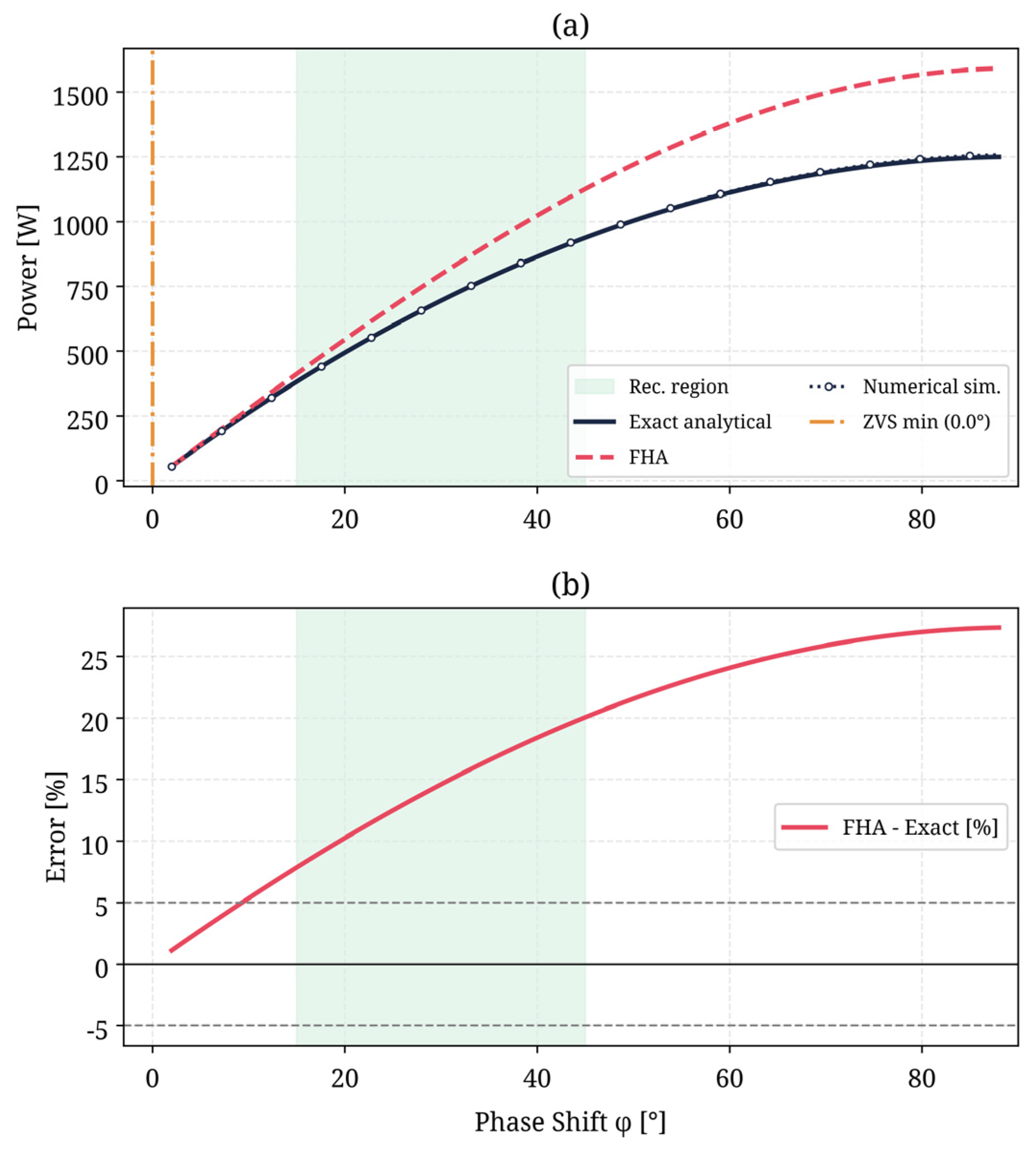
This error reaches 7.9% at φ = 15°, 14.6% at 30°, 20.0% at 45°, and 27.3% at 90°.

Within the investigated SPS range, the FHA always overestimates the transferred power, and the deviation increases with the phase shift [8,10]. This growing discrepancy may reduce the accuracy of control-oriented models relying exclusively on FHA-based power estimation.

4. Operating Constraints

4.1. Loss and Thermal Model

The conduction loss is calculated as:

$$P_{cond}=I_{rms }^2{R}_{eq}$$

A ZVS-aware switching loss:

$$P_{\mathrm{s}\mathrm{w}}=\{\begin{array}{cc}{\alpha }_{\mathrm{Z}\mathrm{V}\mathrm{S}}{ P}_{\mathrm{s}\mathrm{w},\mathrm{h}\mathrm{a}\mathrm{r}\mathrm{d}},& \varphi \ge {\varphi }_{\mathrm{Z}\mathrm{V}\mathrm{S},\mathrm{m}\mathrm{i}\mathrm{n}},\\ P_{\mathrm{s}\mathrm{w},\mathrm{h}\mathrm{a}\mathrm{r}\mathrm{d}},& \varphi <{\varphi }_{\mathrm{Z}\mathrm{V}\mathrm{S},\mathrm{m}\mathrm{i}\mathrm{n}}.\end{array}$$

For the baseline analysis, a residual ZVS-loss factor of 5% of the corresponding hard-switching loss is adopted as a nominal engineering approximation:

$$P_{sw}=0.05P_{sw,hard, }\varphi \ge {\varphi }_{zvs,min}$$

Whereas

$$P_{sw}=P_{sw,hard}, \varphi <{\varphi }_{zvs,min}$$

where $P_{sw,hard}$ is estimated using the loss-modeling method in [6,7]. The values R_eq = 50 mΩ and ${\alpha }_{ZVS}$ = 0.05 are treated as nominal lumped baseline parameters. Their physical basis and quantitative sensitivity are discussed in Appendix A.1 and Appendix A.2.

The junction temperature is calculated as:

$$T_j=T_a+(P_{cond}+P_{sw})R_{th,ja}$$

where $T_a$ is the ambient temperature and $R_{th,ja}$ is the junction-to-ambient thermal resistance.

Thermal compliance requires:

$$T_j\le {125}^{\circ }\mathrm{C}$$

According to the thermal constraint, the value of the junction temperature should not exceed 125 °C. The ambient temperature in this analysis is assumed to be $T_a={40}^{\circ }\mathrm{C}$ while the $R_{th,ja}={20}^{\circ }\mathrm{C}/\mathrm{W}$; thus, the maximal allowed power loss is about 4.25 W.

4.2. ZVS Boundary

Applying the SPS switching-current polarity condition for ZVS [5,12,14,15], the minimum phase shift required for ZVS is

$${\varphi }_{\mathrm{Z}\mathrm{V}\mathrm{S},\mathrm{m}\mathrm{i}\mathrm{n}}={\displaystyle \frac{\pi }{2}}\mathrm{m}\mathrm{a}\mathrm{x}(0,1-k).$$

For the nominal case $k=1.0$, this analytical criterion gives

$${\varphi }_{\mathrm{Z}\mathrm{V}\mathrm{S},\mathrm{m}\mathrm{i}\mathrm{n}}=0^{\circ }.$$

As the voltage ratio decreases below unity, the minimum phase shift required for ZVS increases. For illustration,

$${\varphi }_{\mathrm{Z}\mathrm{V}\mathrm{S},\mathrm{m}\mathrm{i}\mathrm{n}}={13.5}^{\circ }\mathrm{at} k=0.85,$$

and

$${\varphi }_{\mathrm{Z}\mathrm{V}\mathrm{S},\mathrm{m}\mathrm{i}\mathrm{n}}={27}^{\circ }\mathrm{at} k=0.70.$$

Consequently, a decreasing voltage ratio progressively restricts the admissible operating region by tightening the ZVS constraint [12,16].

4.3. Operating Region Synthesis

The interval φ ∈ [15°,45°] is considered as a broader design-assessment range over k ∈ [0.70,1.30], rather than as a universally feasible operating band. For the baseline parameters, the binding thermal upper limit is approximately φ = 35° at k = 1.0; operation toward 45° requires reduced equivalent resistance and/or improved thermal management.

5. Results and Discussion

All computational workflow and simulations were implemented in Python 3.12.3 using NumPy 2.5.1, with Matplotlib 3.11.1 used for visualization and generation of the final production figures. The time-domain simulator applies the exact piecewise ODE solution within each switching segment, while the steady-state initial condition is determined numerically using a bisection-based periodicity solver. The phase shift was swept over φ ∈ [2°,88°] in 87 steps.

At the baseline k = 1.0, Table 3 summarizes the key simulation results.

Table 3. Simulation results at baseline k = 1.0 (V₁ = V₂ᵣ = 100 V, L = 20 μH, f_s = 50 kHz). ✗ = thermal violation.

Metric	φ = 15°	φ = 30°	φ = 45°	φ = 88°
Exact power $P_{\mathrm{e}\mathrm{x}\mathrm{a}\mathrm{c}\mathrm{t}}$ [W]	381.9	694.4	937.5	1249.4
FHA power [W]	411.9	795.8	1125.4	1590.6
FHA error ε [%]	7.85	14.59	20.04	27.31
Irms analytical [A]	4.05	7.86	11.41	20.07
Conduction loss [W]	0.82	3.09	6.51	20.14
Junction temp Tj [°C]	56.8 °C	102.1 °C	170.6 °C ✗	443.2 °C ✗
Efficiency η [%]	99.78	99.55	99.31	98.41

5.1. Power Transfer Validation (Figure 1)

Figure 1a plots the exact analytical power, FHA power, and the numerical simulation for k = 1.0. The numerical model is close to the exact one; the error between them is within a 1.5% margin. Figure 1b depicts how the FHA error rises above 5% at $\varphi$ ≈ 9° and then grows up to 27.3% at $\varphi$ ≈ 88°, indicating that a feedforward steady-state correction may be beneficial for FHA-based controllers operating in this region.

The analytical SPS power reaches its theoretical maximum at $\varphi ={90}^{°}$, whereas the numerical sweep was limited to $\varphi ={88}^{°}$.

Figure 1. Power-transfer characteristic (a) and FHA error (b) at $(k=1.0)$. The shaded green band denotes the broader design-assessment range, φ ∈ [15°,45°], and does not imply thermal feasibility over the entire interval. The dashed horizontal lines in (b) indicate the ±5% FHA-error thresholds.

Figure 1. Power-transfer characteristic (a) and FHA error (b) at $(k=1.0)$. The shaded green band denotes the broader design-assessment range, φ ∈ [15°,45°], and does not imply thermal feasibility over the entire interval. The dashed horizontal lines in (b) indicate the ±5% FHA-error thresholds.

5.2. RMS Current and Loss Breakdown (Figure 2)

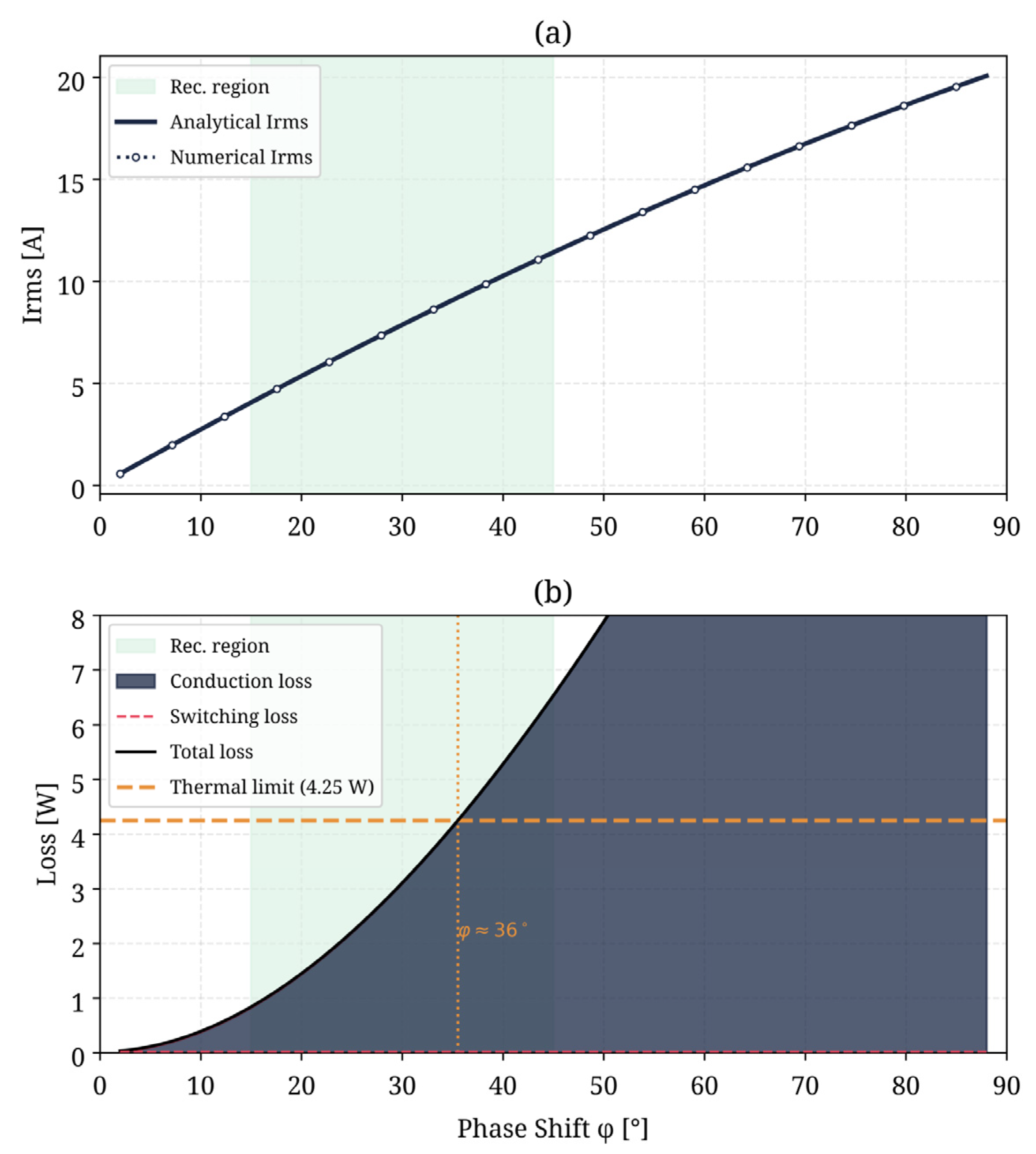
Figure 2a shows that Irms rises from 4.05 A at φ = 15° to 20.07 A at φ = 88° representing an approximately fivefold increase and, consequently, about a 25-fold increase in conduction loss. Figure 2b shows the loss breakdown.

At $k=1.0$, the adopted analytical ZVS criterion is satisfied throughout the investigated phase-shift range, and conduction loss dominates near the thermal boundary. The 4.25 W thermal budget was exceeded between φ ≈ 35° and 36°, with T_j reaching 170.6 °C at φ = 45° and 443.2 °C at φ = 88°.

Figure 2. RMS current and loss breakdown: (a) analytical and numerical Irms with ZVS boundary; (b) conduction and switching losses with thermal budget limit (4.25 W, dashed).

Figure 2. RMS current and loss breakdown: (a) analytical and numerical Irms with ZVS boundary; (b) conduction and switching losses with thermal budget limit (4.25 W, dashed).

5.3. Time-Domain Waveforms (Figure 3)

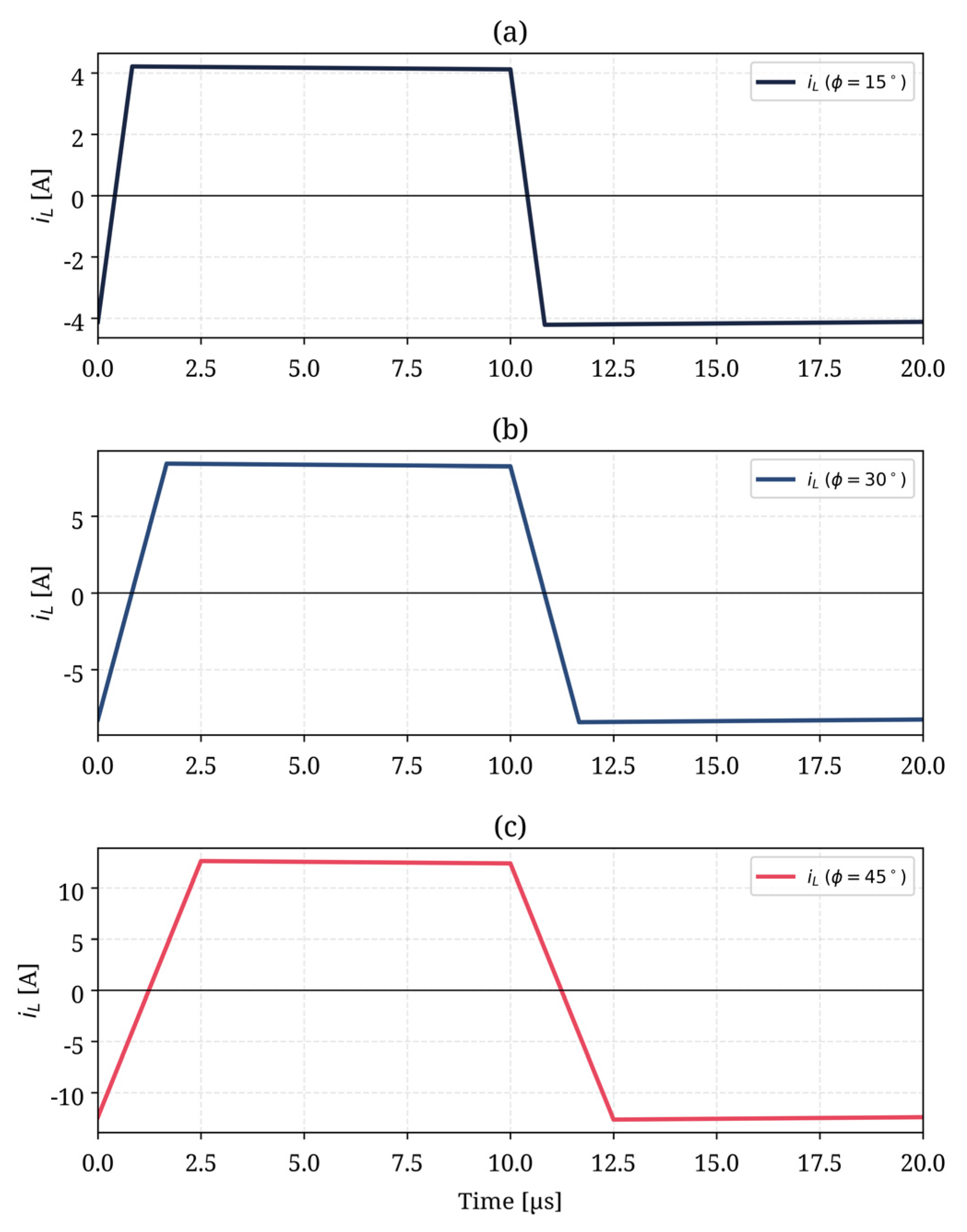
Figure 3 plots the steady-state inductor current at representative phase shifts of 15°, 30°, and 45° for the baseline parameters ($V_1 = V_{2r} = 100$ V). The current waveform remains piecewise linear, while its amplitude increases substantially with phase shift. At $\varphi =$ 45°, the peak-current magnitude approaches approximately 12.5 A. The increasing current amplitude is consistent with the rise in $I_{\mathrm{r}\mathrm{m}\mathrm{s}}$ and conduction loss observed in Figure 2, while the incremental transferred-power gain decreases as the SPS power characteristic approaches its theoretical maximum.

Figure 3. Time-domain inductor-current waveforms at key operating points (V₁ = V₂ᵣ = 100 V): (a) φ = 15°, P = 381.9 W; (b) φ = 30°, P = 694.4 W; (c) φ = 45°, P = 937.5 W.

Figure 3. Time-domain inductor-current waveforms at key operating points (V₁ = V₂ᵣ = 100 V): (a) φ = 15°, P = 381.9 W; (b) φ = 30°, P = 694.4 W; (c) φ = 45°, P = 937.5 W.

5.4. Voltage Ratio Sweep (Figure 4)

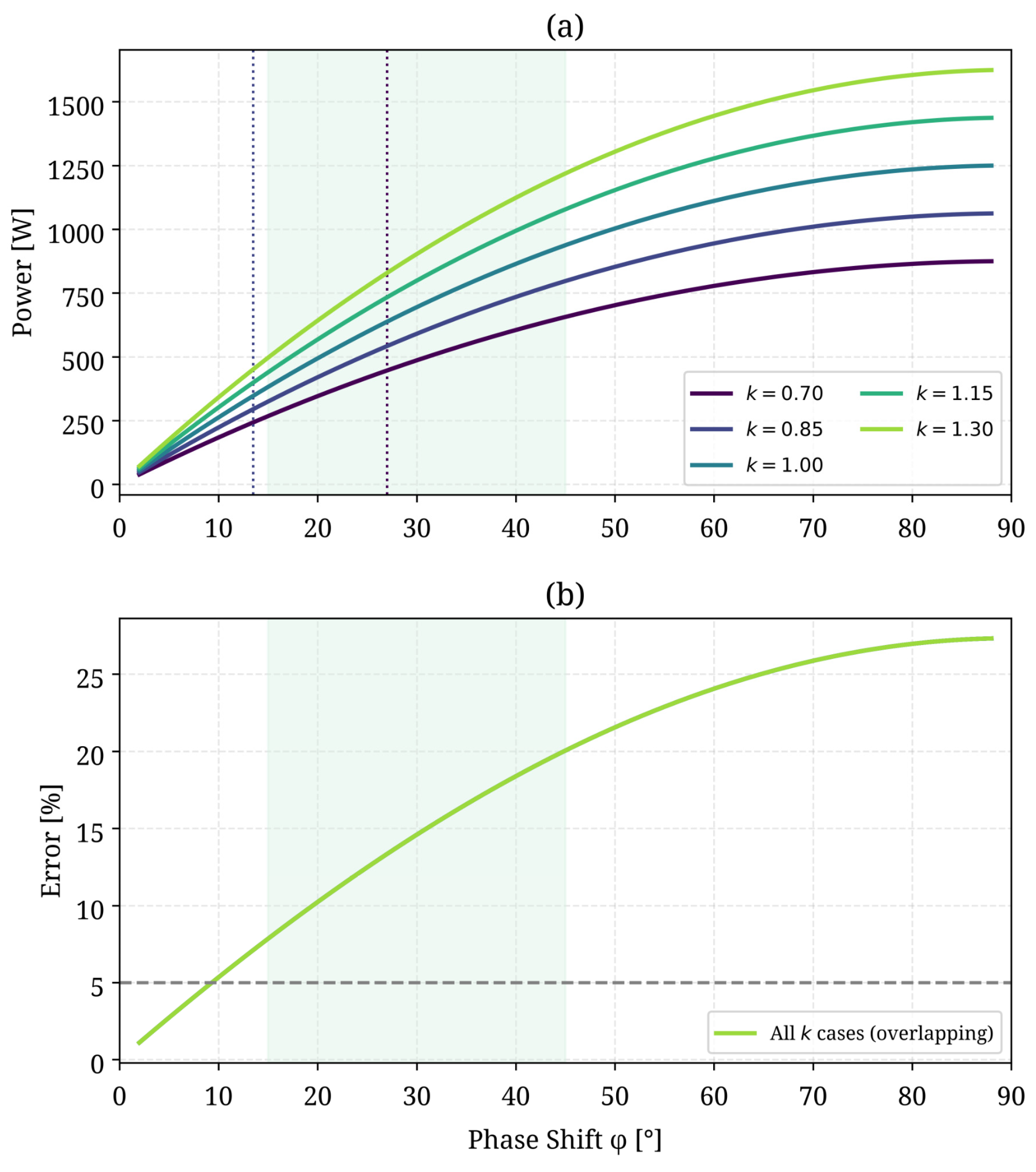
Figure 4 shows the power curves and FHA error for k ∈ {0.70, 0.85, 1.00, 1.15, 1.30}.

The lower values of $k$ lead to decrease in the absolute power transferred, but the phase-shift normalized dependence has the same mathematical expression. The minimum value of the phase shift required by the adopted ZVS criterion changes from $0^{°}$ at $k\ge 1.0$to ${27}^{°}$ ($k=0.70)$, as indicated by the vertical dashed lines in Figure 4a.

The FHA percentage-error curves coincide for the investigated voltage ratios because, under the ideal SPS analytical formulation adopted here, the common voltage-product term V₁V₂ᵣ cancels from the relative-error expression. Consequently, the relative FHA error depends on phase shift φ but is independent of k, although the absolute transferred power, RMS current, ZVS boundary, and thermal feasibility remain k-dependent (full derivation in Appendix A.3).

Figure 4. Voltage ratio parameter sweep k ∈ {0.70, 0.85, 1.00, 1.15, 1.30}: (a) power-transfer curves; the dotted vertical lines indicate the ZVS minimum phase-shift boundaries; (b) FHA percentage error; the dashed horizontal line indicates the 5% error threshold.

Figure 4. Voltage ratio parameter sweep k ∈ {0.70, 0.85, 1.00, 1.15, 1.30}: (a) power-transfer curves; the dotted vertical lines indicate the ZVS minimum phase-shift boundaries; (b) FHA percentage error; the dashed horizontal line indicates the 5% error threshold.

5.5. Shape-Invariance Under L and f_s (Figure 5)

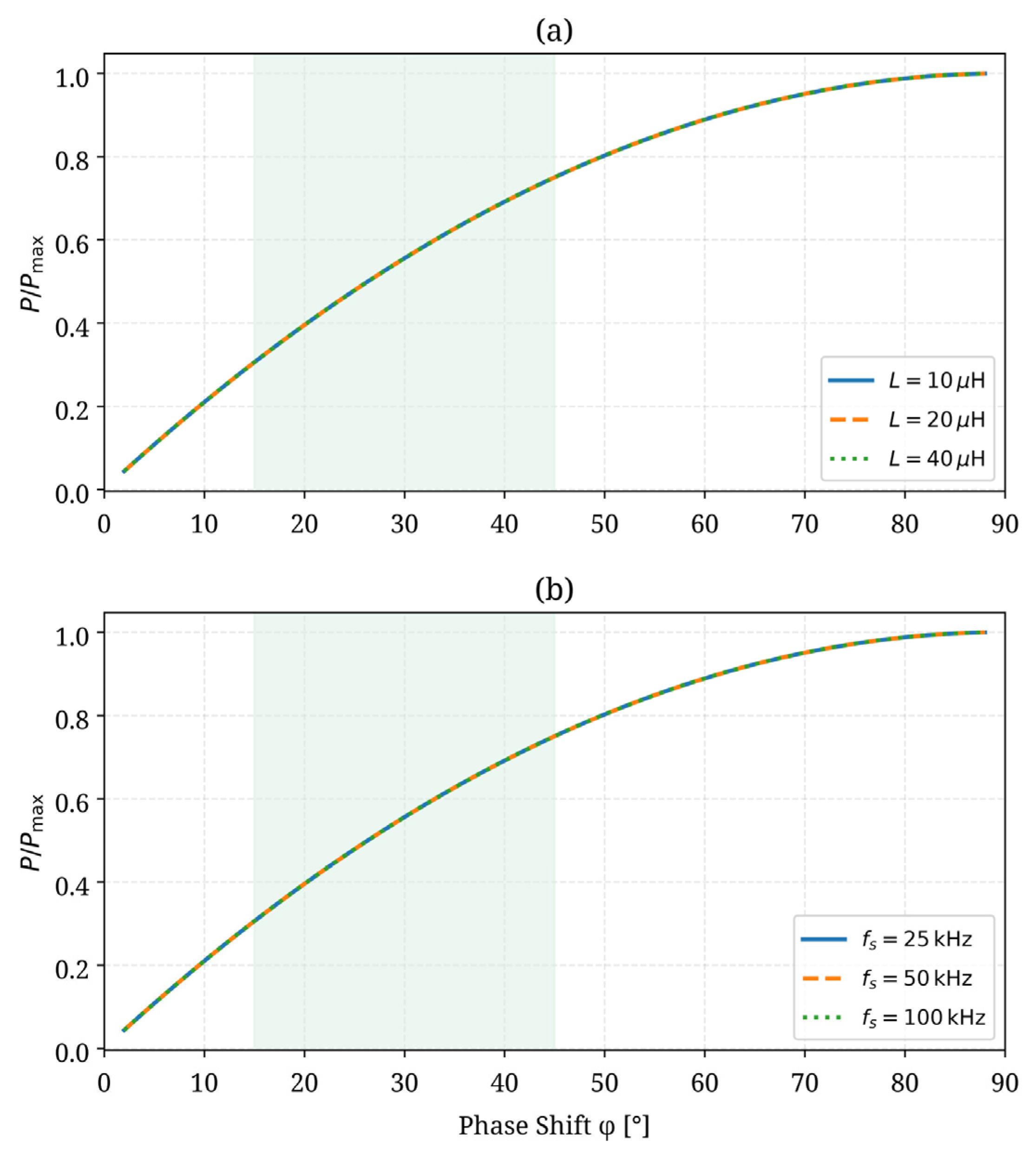
Although the normalized power-transfer curve retains the same shape under variations in L and f_s, the RMS current, losses, and the resulting thermal feasibility boundary remain parameter-dependent and must be reassessed for a specific converter design.

Figure 5. Normalized power P/P_max demonstrating shape-invariance: (a) inductance sweep L ∈ {10, 20, 40 μH}; (b) switching frequency sweep f_s ∈ {25, 50, 100 kHz}. All curves coincide.

Figure 5. Normalized power P/P_max demonstrating shape-invariance: (a) inductance sweep L ∈ {10, 20, 40 μH}; (b) switching frequency sweep f_s ∈ {25, 50, 100 kHz}. All curves coincide.

5.6. Generalized 2D Operating Map (Figure 6)

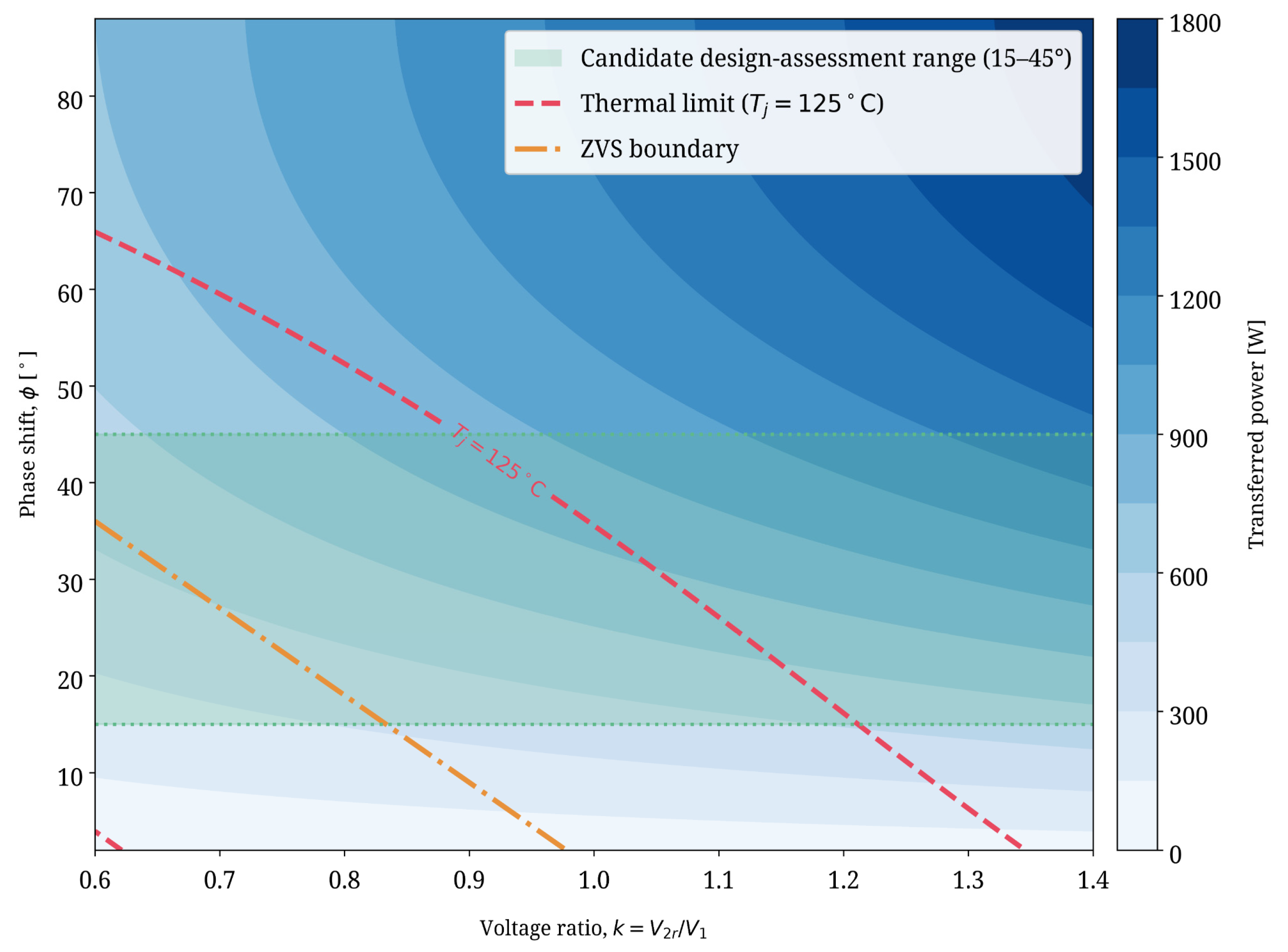
The (k, φ) chart in Figure 6 is the key design aid used in this investigation. The (k, φ) map shows the power contours (colored field), thermal limit (red dashed line, T_j = 125 °C), ZVS boundary (orange dash-dot line, φ = 90°·(1 − k)), and broader candidate design-assessment range (green band). The analysis of the map shows (i) the thermal limit to be the binding upper constraint for the entire range of k, (ii) the ZVS region to overlap with the broader candidate design-assessment range at around k = 0.83, (iii) medium-power operation points are possible within a relatively wide range of studied voltage ratio values, assuming the simultaneous fulfillment of ZVS and thermal limits; and (iv) decreasing k leads to the decrease in the maximum transferable power as well as to the tightening of ZVS lower boundary, while increase in k can make the thermal limit more stringent under the nominal parameter values ($R_{\mathrm{e}\mathrm{q}}=50$ mΩ).

Figure 6. Generalized operating map over the (k, φ) plane: power [W] (color), thermal limit T_j = 125 °C (red dashed), ZVS boundary (orange dash-dot), and broader candidate design-assessment range φ ∈ [15°, 45°] (green band).

Figure 6. Generalized operating map over the (k, φ) plane: power [W] (color), thermal limit T_j = 125 °C (red dashed), ZVS boundary (orange dash-dot), and broader candidate design-assessment range φ ∈ [15°, 45°] (green band).

5.7. Efficiency Analysis (Figure 7)

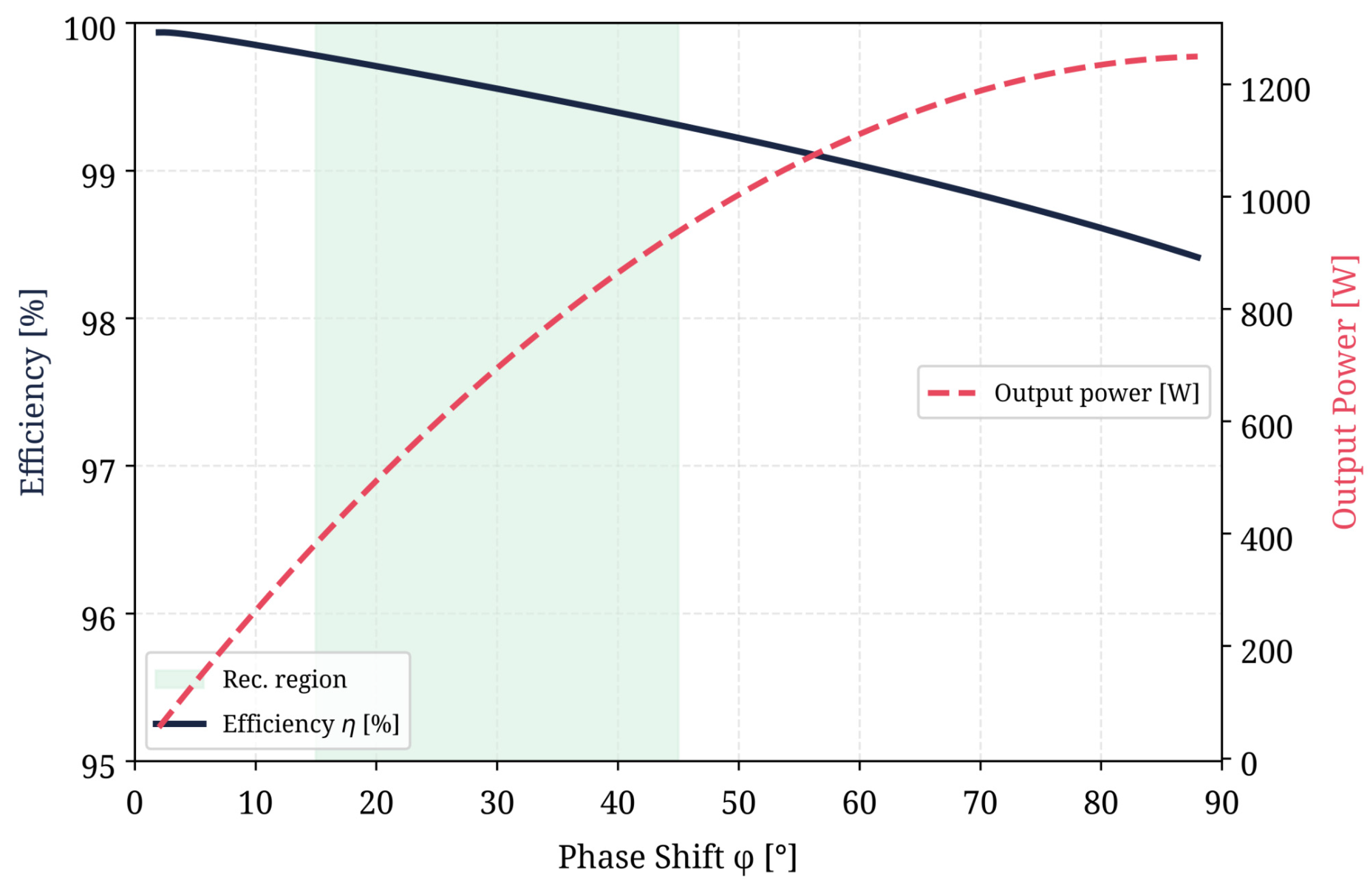
Figure 7 shows the converter efficiency and output power versus the phase shift. The efficiency is the highest at low phase shift and decreases gradually as the phase shift increases, illustrating that the efficiency and power-optimal operating points are distinct. Efficiency remains above 99% throughout the broader candidate design-assessment range; however, efficiency alone does not establish feasibility, because the baseline thermal constraint becomes binding at approximately 35°.

Figure 7. Converter efficiency (solid) and output power (dashed) vs. phase shift with the broader candidate design-assessment range highlighted.

Figure 7. Converter efficiency (solid) and output power (dashed) vs. phase shift with the broader candidate design-assessment range highlighted.

5.8. Parametric Sensitivity and Robustness Assessment

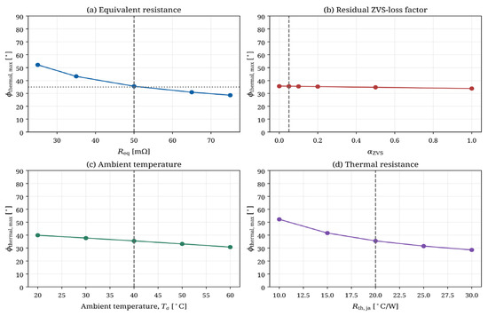
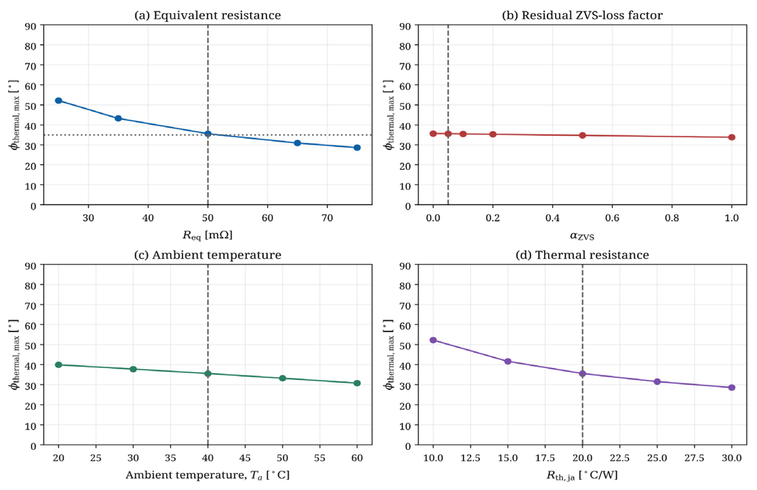
To evaluate robustness against parameter variations, parametric sensitivity analyses were performed on the equivalent series resistance R_eq, residual ZVS-loss factor α_ZVS, ambient temperature T_a, and thermal resistance $R_{th,ja}$ In the baseline model, R_eq = 50 mΩ and α_ZVC = 0.05 are treated as lumped nominal parameters. The results in Figure 8 show two distinct sensitivity trends. The thermal boundary is strongly affected by R_eq and the thermal parameters: increasing the effective conduction resistance contracts the feasible upper phase-shift range, whereas reducing it extends the admissible range. Accordingly, operation toward 45° under the present design requires lower effective hot resistance and/or improved thermal management. Increasing T_a from 40 °C to 60 °C reduces ${\varphi }_{\mathrm{t}\mathrm{h}\mathrm{e}\mathrm{r}\mathrm{m}\mathrm{a}\mathrm{l},\mathrm{m}\mathrm{a}\mathrm{x}}$from approximately 35.5° to 30.7°, whereas reducing $R_{th,ja}$from 20 °C/W to 10 °C/W expands the boundary to approximately 52.2°. These results demonstrate that the nominal 15–35° interval is a baseline case-study result rather than a universal spacecraft operating interval.

Figure 8. Parametric sensitivity of maximum thermal phase shift ${\varphi }_{\mathrm{t}\mathrm{h}\mathrm{e}\mathrm{r}\mathrm{m}\mathrm{a}\mathrm{l},\mathrm{m}\mathrm{a}\mathrm{x}}$ against equivalent series resistance $R_{eq}$ (a), residual ZVS factor ${\alpha }_{\mathrm{Z}\mathrm{V}\mathrm{S}}$ (b), ambient temperature $T_a$ (c), and thermal resistance $R_{th,ja}$ (d). The vertical dashed lines indicate the nominal baseline values $R_{\mathrm{e}\mathrm{q}}=50\hspace{0.17em}\mathrm{m}\mathsf{\Omega }$, ${\alpha }_{\mathrm{Z}\mathrm{V}\mathrm{S}}=0.05$, $T_a={40 }^{ \circ }\mathrm{C}$, and $R_{th,ja}={20 }^{\circ }\mathrm{C}/\mathrm{W}$. The horizontal dotted line in panel (a) indicates the nominal thermal-boundary reference.

By contrast, within the sensitivity interval ${\alpha }_{ZVS}\in [0,0.20]$, the change in ${\varphi }_{\mathrm{t}\mathrm{h}\mathrm{e}\mathrm{r}\mathrm{m}\mathrm{a}\mathrm{l},\mathrm{m}\mathrm{a}\mathrm{x}}$ is less than approximately 0.5°. Figure 8b additionally shows the broader parametric trend up to ${\alpha }_{ZVS}=1.0$. Thus, within the present baseline loss model, the thermal boundary is considerably more sensitive to conduction resistance and thermal conditions than to the assumed residual ZVS-loss factor. Figure 8 should therefore be interpreted as a parametric sensitivity envelope rather than as a transient orbital thermal simulation.

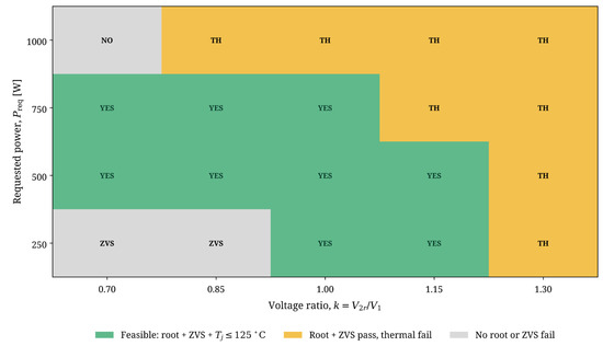
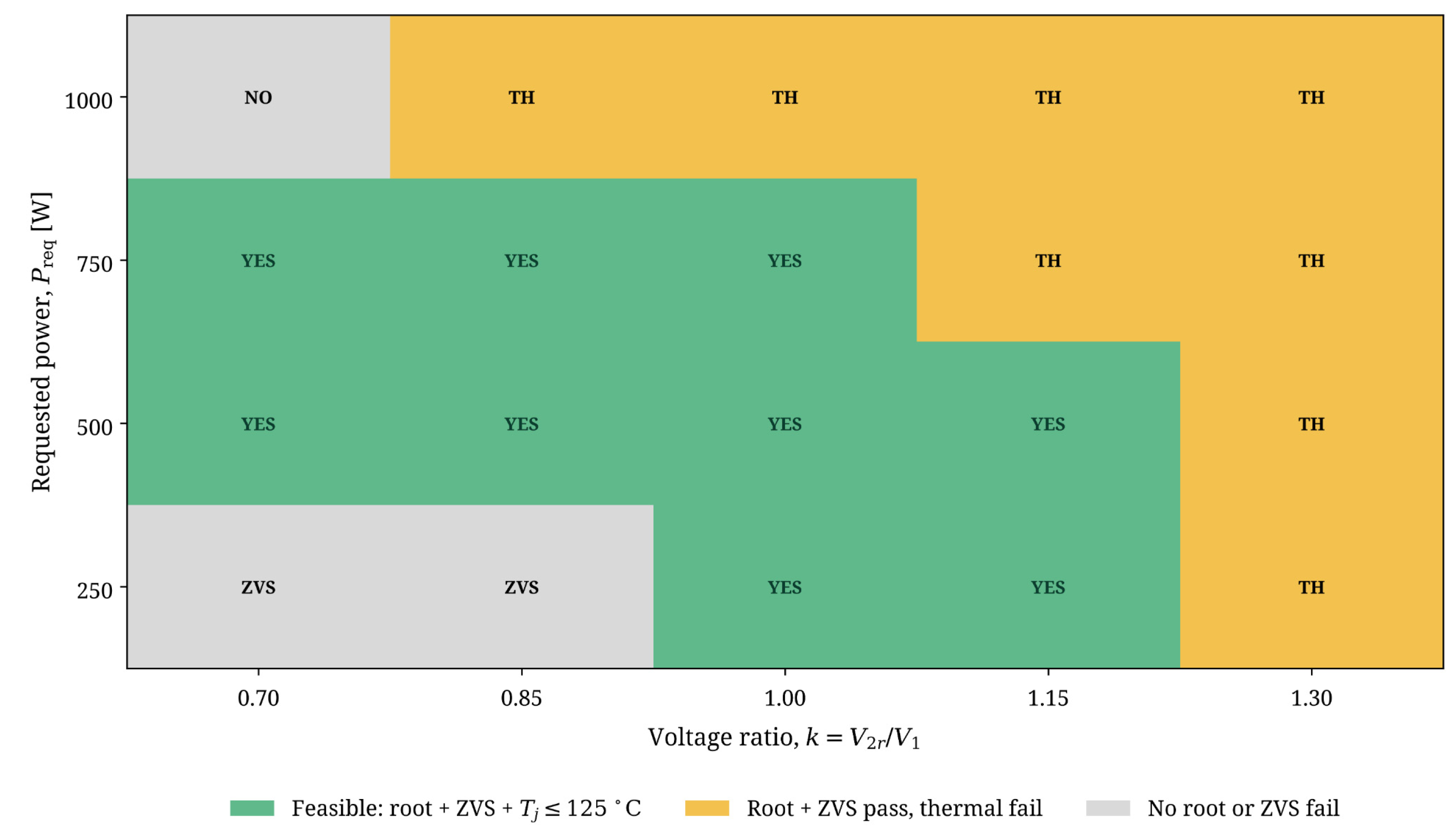
Furthermore, evaluation of variable bus voltage (k ∈ [0.70, 1.30]) and load-power demands from 250 W to 1000 W using the exact lower SPS phase root shows that the admissible operating set must be determined from the exact power-transfer relation together with the independent ZVS (φ ≥ φ_ZVS,min(k)) and thermal (T_j ≤ 125 °C) constraints rather than by applying a fixed phase-shift command. If no admissible SPS power root exists, or if either the ZVS or thermal constraint is violated, the requested operating point is infeasible and the requested power must be reduced or otherwise modified and reevaluated.

Figure 9 illustrates this strict k- and load-dependent feasibility assessment.

Figure 9. Strict feasible operating status map across voltage ratio k and load power demands Preq, derived from exact lower SPS phase roots, independent ZVS verification, and thermal limits.

The detailed physical justification of the R_eq and residual-loss assumptions is retained in Appendix A.1 and Appendix A.2, respectively. The closed-form feasibility procedure and the interpretation of variable spacecraft thermal conditions are provided in Appendix A.4 and Appendix A.5.

6. Spacecraft EPS Design Implications

R1: The converter components should therefore be sized to deliver the required operating power within the applicable feasible phase-shift interval determined by the thermal and ZVS constraints. For spacecraft implementation, these converter-level design considerations should be integrated within the broader spacecraft electrical and electronic engineering framework specified by ECSS-E-ST-20C Rev.2 [17].

R2: Figure 6 uses the voltage ratio k as a parameter to characterize converter operation under changing bus-voltage conditions. As k departs from unity, the feasible operating region changes because the ZVS lower boundary and thermal upper boundary shift. Therefore, practical spacecraft EPS control should account for the instantaneous voltage ratio when determining the admissible phase-shift command.

R3: The equivalent series resistance R_eq aggregates semiconductor on-state resistance and transformer winding/conductor losses. Because R_eq directly governs conduction loss and the resulting thermal upper boundary, careful device selection and low-loss winding construction are essential for extending the feasible operating range.

For a specified maximum phase shift ${\varphi }_{\mathrm{m}\mathrm{a}\mathrm{x}}$, a first-order conduction-dominated resistance target is

$$R_{\mathrm{e}\mathrm{q}}\le {\displaystyle \frac{P_{\mathrm{l}\mathrm{o}\mathrm{s}\mathrm{s},\mathrm{m}\mathrm{a}\mathrm{x}}}{I_{\mathrm{r}\mathrm{m}\mathrm{s}}^2\left({\varphi }_{\mathrm{m}\mathrm{a}\mathrm{x}}\right)}},$$

where $P_{\mathrm{l}\mathrm{o}\mathrm{s}\mathrm{s},\mathrm{m}\mathrm{a}\mathrm{x}}$ is the allowable total-loss budget under the adopted thermal model.

When the residual switching-loss term is retained explicitly, the corresponding limit becomes

$$R_{\mathrm{e}\mathrm{q}}\le {\displaystyle \frac{P_{\mathrm{l}\mathrm{o}\mathrm{s}\mathrm{s},\mathrm{m}\mathrm{a}\mathrm{x}}-P_{\mathrm{s}\mathrm{w}}\left({\varphi }_{\mathrm{m}\mathrm{a}\mathrm{x}}\right)}{I_{\mathrm{r}\mathrm{m}\mathrm{s}}^2\left({\varphi }_{\mathrm{m}\mathrm{a}\mathrm{x}}\right)}}$$

These relations provide direct design targets for the combined semiconductor on-state and winding/conductor resistance.

R4: The closed-form framework can be used as a supervisory feasibility evaluator rather than implementing the baseline phase-shift interval as a universal fixed command range. For updated bus voltages, requested power, and applicable thermal parameters, the supervisory layer computes the lower SPS phase-shift root from the exact power-transfer relation and independently verifies the ZVS and thermal constraints, as detailed in Appendix A.4. The operating point is accepted only when an admissible SPS phase-shift root exists and all ZVS and thermal constraints are satisfied; otherwise, the requested power should be reduced or otherwise modified and reevaluated rather than forcing the phase shift to a constraint boundary. This constitutes a steady-state supervisory feasibility evaluation; transient thermal dynamics and mission-specific implementation remain subjects for future work.

7. Conclusions

This study presents a physics-informed framework for the operating-region design of DAB converters for spacecraft EPS. The exact RMS expression agrees with the independent time-domain simulation within 1.3%, providing a consistent basis for the loss and thermal calculations. The FHA overestimates transferred power by 7.9% at φ = 15°, increasing to 20.0% at φ = 45° across the broader design-assessment range and reaching 27.3% at φ = 90°. The thermal constraint is the most restrictive upper bound for the baseline case (φ ≈ 35° at k = 1.0). The generalized 2D map provides a single design tool that presents the power, ZVS, and thermal constraint boundaries simultaneously. The normalized power-transfer curve retains the same shape under variations in L and fs; however, the RMS current, losses, and resulting thermal feasibility boundary remain parameter-dependent and must be reassessed for each specific converter design. Maximum power transfer at φ = 90° is incompatible with the adopted baseline thermal limit, with the calculated junction temperature far above the 125 °C limit. Future work will extend the framework to dual-phase-shift modulation and include physical-prototype validation of the predicted operating-region boundaries (Appendix A.6).

Appendix A.1. Temperature and Operating-Point Dependence of the Equivalent Series Resistance

The physical equivalent resistance is not generally constant over the complete temperature and current operating range. In the present model, R_eq = 50 mΩ is a nominal lumped baseline parameter used to quantify the baseline thermal boundary; it is not intended to represent a universal temperature-independent device property. It represents the aggregate conduction path, comprising the primary-side semiconductor resistance, the secondary-side semiconductor resistance referred to the primary side, and the transformer winding/conductor losses (Section 6, R3):

$$R_{eq}=R_{sw,pri}+n^2{R}_{sw,sec}+R_{xfmr}$$

The dominant physical variation in the semiconductor term is its junction-temperature dependence, described to first order by

$$R_{ds\left(on\right)}\left(T_j\right)=R_{ds\left(on\right),25{}^{\circ }\mathrm{C}}\cdot \left[1+\alpha \left(T_j-25{}^{\circ }\mathrm{C}\right)\right]$$

with a typical positive temperature coefficient α ≈ 0.3–0.5%/°C for silicon power MOSFETs [18]. The effective winding contribution additionally depends on the current waveform and on frequency-dependent conductor losses through skin and proximity effects [19]. The actual effective resistance may therefore vary with temperature and operating point.

To quantify the consequence of this variation without introducing a complete device-level electro-thermal model, a sensitivity analysis of R_eq over 25–75 mΩ was performed (Section 5.8, Figure 8a). The results show directly how the thermal phase-shift boundary shifts as the lumped equivalent resistance changes.

We also retain the first-order design relation of recommendation R3,

$$R_{eq}\le {\displaystyle \frac{P_{loss,max}}{I_{rms}^2\left({\phi }_{max}\right)}}$$

as a conduction-dominated resistance target for a specified operating point. For the 45° candidate-assessment point, this relation gives approximately 32.7 mΩ using the baseline RMS current (11.41 A, Table 3) and the stated thermal-loss budget (4.25 W). When the residual switching-loss term of the complete model is included, the allowable resistance is lower still. These calculations provide the technical basis for the engineering interpretation summarized in Section 5.8: the 45° candidate-assessment point is not thermally feasible for the nominal 50 mΩ baseline design, and operation toward it requires lower effective hot resistance and/or improved thermal management. A self-consistent temperature-dependent and harmonic-resolved electro-thermal model remains beyond the present scope.

Appendix A.2. Physical Basis of the Residual Switching-Loss Factor α_ZVS = 0.05

Under complete zero-voltage switching, capacitive turn-on loss is substantially reduced because the device output capacitance is discharged by the commutation current before turn-on. Nevertheless, nonzero switching losses may remain because of nonideal device capacitances, turn-off transitions, and incomplete soft switching near the ZVS boundary. These mechanisms have been analytically described and experimentally demonstrated in [20] and are consistent with the DAB loss-modeling approaches in [6,7]. In the present study, α_ZVS = 0.05 is therefore treated as a nominal engineering approximation rather than a universal device-independent constant. The sensitivity analysis shows that, within ${\alpha }_{ZVS}\in [0,0.20]$, the thermal boundary ${\varphi }_{\mathrm{t}\mathrm{h}\mathrm{e}\mathrm{r}\mathrm{m}\mathrm{a}\mathrm{l},\mathrm{m}\mathrm{a}\mathrm{x}}$ shifts by less than ${0.5}^{°}$; Figure 8b additionally shows the broader parametric trend up to ${\alpha }_{ZVS}=1.0$. The corresponding engineering implication is summarized in Section 5.8, while the present subsection provides the physical basis and quantitative bounding of the residual-loss assumption.

Appendix A.3. Analytical k-Independence of the Relative FHA Error

From the exact SPS power expression and its first-harmonic approximation (Section 3.3), the relative FHA error is:

$${\epsilon }_{FHA}={\displaystyle \frac{P_{FHA}-P_{exact}}{P_{exact}}}\times 100\%=\left[{\displaystyle \frac{\pi \mathrm{s}\mathrm{i}\mathrm{n}\phi }{\phi \left(\pi -\phi \right)}}-1\right]\times 100\%$$

The common voltage product V₁V_2r cancels identically between numerator and denominator.

Consequently, under the ideal SPS formulation the relative FHA error depends only on the phase shift φ and is independent of the voltage-conversion ratio $k$, and therefore of both the sign of the voltage mismatch ($k <1$ versus $k >1$) and its magnitude. This is confirmed by the coinciding error curves in Figure 4b, and evaluation of the closed form reproduces the tabulated values (7.85% at φ = 15° and 20.04% at φ = 45°, Table 3). This conclusion is confined to the ideal, lossless SPS formulation adopted for the FHA comparison and to forward power transfer over 0 ≤ φ ≤ π. Nonideal effects—device output capacitance, dead time, unequal semiconductor drops, winding resistance, and transformer parasitics—and reverse-power operation, which requires a port-oriented sign convention and the magnitude form of the phase-shift argument, may introduce additional k-dependence and lie outside the present validation. The voltage ratio nevertheless governs the absolute transferred power, RMS current, ZVS boundary, conduction loss, and thermal feasibility, all of which remain strongly k-dependent.

Appendix A.4. Online Evaluation of the Feasible Operating Point

Under variable bus-voltage and load conditions, the measured voltages define k = V_2r/V₁ and the requested transferred power is denoted by $P_{\mathrm{r}\mathrm{e}\mathrm{q}}$. The required phase shift is obtained from the lower root of the exact SPS power-transfer relation, with $P^{*}\equiv P_{\mathrm{r}\mathrm{e}\mathrm{q}}$ in the expression below:

$${\phi }^{\mathrm{*}}={\displaystyle \frac{\pi }{2}}\left[1-\sqrt{1-{\displaystyle \frac{8f_{s}L{P}^{\mathrm{*}}}{V_1{V}_{2r}}}}\right]$$

The lower root exists provided

$$0\le P_{\mathrm{r}\mathrm{e}\mathrm{q}}\le {\displaystyle \frac{V_1{V}_{2r}}{8f_{s}L}}$$

The resulting ${\varphi }_{\mathrm{r}\mathrm{e}\mathrm{q} }$is then accepted only if the two independent feasibility conditions are satisfied:

(i) ${\varphi }_{\mathrm{r}\mathrm{e}\mathrm{q}}\ge {\varphi }_{\mathrm{Z}\mathrm{V}\mathrm{S},\mathrm{m}\mathrm{i}\mathrm{n}}\left(k\right)$, where

$${\varphi }_{\mathrm{Z}\mathrm{V}\mathrm{S},\mathrm{m}\mathrm{i}\mathrm{n}}\left(k\right)={\displaystyle \frac{\pi }{2}}\mathrm{m}\mathrm{a}\mathrm{x}(0,1-k),$$

from Section 4.2; and

(ii) $T_j({\varphi }_{\mathrm{r}\mathrm{e}\mathrm{q}},k)\le {125}^{\circ }\mathrm{C}$ from the loss and thermal model of Section 4.1. If no admissible lower SPS phase-shift root exists, or if either feasibility condition is violated, the requested operating point is classified as infeasible under the imposed constraints and the supervisory controller must reduce or otherwise modify the requested power rather than forcing the phase shift to a constraint boundary. Equivalently, the strict feasibility map of Figure 9 can be precomputed offline over the (k, $P_{req}$) grid and stored as a lookup table indexed by the measured bus voltages and requested power.

The nominal power-to-phase inversion is available in closed form, and the lookup-table implementation further reduces online computation to interpolation.

Appendix A.5. Parametric Interpretation of Variable Spacecraft Thermal Conditions

Spacecraft thermal boundary conditions can vary with solar flux, eclipse transitions, vehicle attitude, and the available heat-rejection path [21]. In the present model, T_a = 40 °C and $R_{th,ja}$ = 20 °C/W are lumped baseline parameters rather than a complete transient representation of the spacecraft thermal environment. To quantify how variation in these effective thermal parameters influences the feasible operating region, Section 5.8 treats T_a ∈ [20, 60] °C and $R_{th,ja}$ ∈ [10, 30] °C/W as parametric sensitivity ranges.

Figure 8c,d quantifies the resulting shifts in the thermal upper boundary; the principal numerical engineering interpretation is summarized in Section 5.8. These sweeps should be interpreted as static parametric bounds rather than as a simulated orbital thermal trajectory. The operating-region framework can therefore be reevaluated using mission-specific values or conservative bounds for T_a and $R_{th,ja}$. A fully coupled transient orbital electro-thermal model, including thermal capacitances and time-dependent spacecraft boundary conditions, is beyond the scope of the present study and is identified as future work.

Appendix A.6. Scope of Validation and Pathway to Experimental Verification

The present study is analytical and numerical in scope. The closed-form RMS-current expression was cross-checked against the independent time-domain simulation with an error below 1.3%, while the numerical and exact analytical power-transfer results agree within approximately 1.5% over the investigated phase-shift sweep. These comparisons establish the internal consistency of the analytical framework but do not constitute experimental validation. The individual physical phenomena incorporated in the model, including SPS power transfer, ZVS behavior, and converter loss mechanisms, are based on established DAB formulations reported in the cited literature. Nevertheless, experimental verification of the combined operating-region framework, particularly the predicted thermal and ZVS boundaries, requires a physical prototype. Hardware validation at the studied power level, including converter waveforms, RMS current, losses, device temperature, and experimentally observed feasible operating boundaries, is identified as future work.

References

- Naayagi, R.T.; Forsyth, A.J.; Shuttleworth, R. High-power bidirectional DC–DC converter for aerospace applications. IEEE Trans. Power Electron. 2012, 27, 4366–4379. [Google Scholar] [CrossRef] [Scilit]
- Naayagi, R.T.; Forsyth, A.J.; Shuttleworth, R. Bidirectional control of a dual active bridge DC–DC converter for aerospace applications. IET Power Electron. 2012, 5, 1104–1118. [Google Scholar] [CrossRef] [Scilit]
- Ravindran, R.; Massoud, A.M. State-of-the-Art DC–DC Converters for Satellite Applications: A Comprehensive Review. Aerospace 2025, 12, 97. [Google Scholar] [CrossRef] [Scilit]
- De Doncker, R.W.A.A.; Divan, D.M.; Kheraluwala, M.H. A three-phase soft-switched high-power-density DC/DC converter for high-power applications. IEEE Trans. Ind. Appl. 1991, 27, 63–73. [Google Scholar] [CrossRef] [Scilit]
- Kheraluwala, M.H.; Gascoigne, R.W.; Divan, D.M.; Baumann, E.D. Performance characterization of a high-power dual active bridge DC-to-DC converter. IEEE Trans. Ind. Appl. 1992, 28, 1294–1301. [Google Scholar] [CrossRef] [Scilit]
- Krismer, F.; Kolar, J.W. Accurate power loss model derivation of a high-current dual active bridge converter for an automotive application. IEEE Trans. Ind. Electron. 2010, 57, 881–891. [Google Scholar] [CrossRef] [Scilit]
- Turzyński, M.; Bachman, S.; Jasiński, M.; Piasecki, S.; Ryłko, M.; Chiu, H.-J.; Kuo, S.-H.; Chang, Y.-C. Analytical Estimation of Power Losses in a Dual Active Bridge Converter Controlled with a Single-Phase Shift Switching Scheme. Energies 2022, 15, 8262. [Google Scholar] [CrossRef] [Scilit]
- Shao, S.; Chen, L.; Shan, Z.; Gao, F.; Chen, H.; Sha, D.; Dragičević, T. Modeling and Advanced Control of Dual-Active-Bridge DC–DC Converters: A Review. IEEE Trans. Power Electron. 2022, 37, 1524–1547. [Google Scholar] [CrossRef] [Scilit]
- Hou, N.; Li, Y.W. Overview and Comparison of Modulation and Control Strategies for a Nonresonant Single-Phase Dual-Active-Bridge DC–DC Converter. IEEE Trans. Power Electron. 2020, 35, 3148–3172. [Google Scholar] [CrossRef] [Scilit]
- Bai, H.; Mi, C. Eliminate reactive power and increase system efficiency of isolated bidirectional dual-active-bridge DC–DC converters using novel dual-phase-shift control. IEEE Trans. Power Electron. 2008, 23, 2905–2914. [Google Scholar] [CrossRef] [Scilit]
- Yan, Y.; Gui, H.; Bai, H. Complete ZVS Analysis in Dual Active Bridge. IEEE Trans. Power Electron. 2021, 36, 1247–1252. [Google Scholar] [CrossRef] [Scilit]
- Oggier, G.G.; García, G.O.; Oliva, A.R. Switching control strategy to minimize dual active bridge converter losses. IEEE Trans. Power Electron. 2009, 24, 1826–1838. [Google Scholar] [CrossRef] [Scilit]
- Everts, J. Closed-form solution for efficient ZVS modulation of DAB converters. IEEE Trans. Power Electron. 2017, 32, 7561–7576. [Google Scholar] [CrossRef] [Scilit]
- Xu, F.; Liu, J.; Dong, Z. Minimum Backflow Power and ZVS Design for Dual-Active-Bridge DC–DC Converters. IEEE Trans. Ind. Electron. 2023, 70, 474–484. [Google Scholar] [CrossRef] [Scilit]
- Jin, H.; Pei, Y.; Wang, L.; Wen, J.; Yang, C.; Dong, X. Achieving Rated Power and ZVS for Dual Active Bridge Converter Considering the Interaction of Nonidealities. IEEE Trans. Ind. Electron. 2023, 70, 7867–7878. [Google Scholar] [CrossRef] [Scilit]
- Xu, G.; Sha, D.; Xu, Y.; Liao, X. Dual-Transformer-Based DAB Converter with Wide ZVS Range for Wide Voltage Conversion Gain Application. IEEE Trans. Ind. Electron. 2018, 65, 3306–3316. [Google Scholar] [CrossRef] [Scilit]
- ECSS-E-ST-20C Rev.2; Space Engineering—Electrical and Electronic. European Cooperation for Space Standardization. ESA-ESTEC: Noordwijk, The Netherlands, 2022.
- Baliga, B.J. Fundamentals of Power Semiconductor Devices, 2nd ed.; Springer: Cham, Switzerland, 2019. [Google Scholar]
- Dowell, P.L. Effects of eddy currents in transformer windings. Proc. Inst. Electr. Eng. 1966, 113, 1387–1394. [Google Scholar] [CrossRef] [Scilit]
- Kasper, M.; Burkart, R.M.; Deboy, G.; Kolar, J.W. ZVS of Power MOSFETs Revisited. IEEE Trans. Power Electron. 2016, 31, 8063–8067. [Google Scholar] [CrossRef] [Scilit]
- Gilmore, D.G. (Ed.) Spacecraft Thermal Control Handbook, Volume I: Fundamental Technologies, 2nd ed.; The Aerospace Press: El Segundo, CA, USA, 2002. [Google Scholar]
Disclaimer/Publisher’s Note: The statements, opinions and data contained in all publications are solely those of the individual author(s) and contributor(s) and not of MDPI and/or the editor(s). MDPI and/or the editor(s) disclaim responsibility for any injury to people or property resulting from any ideas, methods, instructions or products referred to in the content. |
© 2026 by the authors. Licensee MDPI, Basel, Switzerland. This article is an open access article distributed under the terms and conditions of the Creative Commons Attribution (CC BY) license.