Illuminant Estimation Based on Augmented Dataset and a Piecewise Neural Network ^†

Abstract

The objective of white balance is to accurately estimate and subsequently eliminate the color of global illumination present in an image. Learning-based methods have gained prominence over statistical approaches due to their typically superior accuracy. However, these methods rely on high-quality, large datasets. The quality of a dataset is intrinsically tied to the volume of knowledge it encapsulates, specifically the uniformity in the distribution of labels. In this study, we expand the dataset by leveraging the camera imaging pipeline. Subsequently, we segment the image into 16 partially overlapping blocks that collectively encompass the entire image. We then propose a rudimentary neural network designed to train these blocks with consistent labels, yielding 16 predictive outcomes that serve as image features. These features are used to capture complex illumination and reflection data within the image. Utilizing these features, we employ a straightforward, fully connected neural network to calculate the color mapping function, thereby correcting the image colors. Experimental results show that the methodology proposed in this paper significantly surpasses existing state-of-the-art color constancy methods.

1. Introduction

Scene illumination is assumed to be global and uniform, implying a single illuminant source within the scene. Cameras employ numerous processing steps to transform the raw RGB sensor response into the final output image. During this process, raw-RGB images are processed via in-built camera algorithms to produce standard RGB (sRGB) images. This transformation involves a series of linear and nonlinear processes that result in the images we perceive as normal. Among these processes, white balance (WB) is important as it facilitates the successful transformation from raw-RGB to sRGB. Additionally, WB significantly impacts the accuracy of other computational processes such as semantic segmentation or object recognition [1]. Therefore, using a linear diagonal matrix, we calculate illuminations to convert raw images into standard ones and establish an accurate color spatial domain. Consequently, accurately estimating scene illumination becomes critical. In this paper, we present our algorithm designed to address this challenge and correct illumination appropriately.

Over the past decade, learning-based methods have gained attraction due to their typically superior accuracy compared with statistics-based approaches. However, the efficacy of this method hinges on both the precision and size of the dataset. In this study, we posit that the most critical factor in the learning-based color constancy method is the knowledge content within the dataset, specifically, the uniformity of label distribution.

In contrast to challenges in computer vision, estimating the color of the light source does not necessitate a specialized network structure. However, it demands rigorous standards for both the volume and quality of datasets, as conventional data augmentation techniques are inappropriate for this task [2]. This paper focuses on data-centric research, exploring two primary directions: firstly, enhancing the dataset through the camera’s processing pipeline, and secondly, developing a streamlined neural network model tailored to the augmented dataset.

We analyze data from two perspectives: an examination of the distribution information inherent in the data, and a study of the output produced by existing pretrained models. The results contribute to the enhancement of the original datasets by eliminating the initial colors and incorporating new stochastic illumination. This process appropriately expands the datasets and broadens their color gamut. Theoretically, this augments the dataset’s knowledge base, enhancing the network’s generalization capability. We randomly segment the image into small blocks, each corresponding to the same color labels. These segments are then used to create a new dataset for establishing an expanded color space. These localized image blocks are particularly rich in color information, which facilitates efficient feature extraction via simple neural networks. A straightforward regression model is used to process the estimated illumination color of each block, thereby obtaining the final illumination color estimation.

2. Related Work

WB is a process designed to replicate the human visual system’s capabilities in machines, specifically by determining the light source of a scene to facilitate subsequent transformations. Consequently, WB is a fundamental yet critical stage, and accurately calculating WB has emerged as a significant challenge. Generally, three methodologies are employed to predict the illuminant of a scene in images. The traditional methods are statistics-based and machine learning-based. A third method was introduced by Mahmoud et al. [3], who proposed a new approach to WB regardless of the original image content. They utilized a k-nearest neighbor strategy to achieve WB after images had been incorrectly white-balanced.

2.1. Statistic-Based Methods

The prediction of scene light sources using statistical methods is primarily achieved by analyzing the distribution of color and brightness information in images. Despite the increasing dominance of learning-based methods in recent years, classic algorithms based on statistical approaches continue to offer enduring benefits. Song [4] employed a traditional method to predict the background light in underwater images, achieving significant success. This method restored the underwater illuminant radiance but also enhanced the contrast, color, and visibility. Additionally, Li [5] addressed the challenge of blurry images in rainy scenes by estimating the exposure time and the duration it takes for a raindrop to traverse a pixel. Cheng [6] delved into the reasons behind the efficacy of spatial domain methods and their relationship with techniques that operate directly in the color domain. They discovered that spatial domain methods benefit from significant gradients in the scene, which correlate with stark color differences in the color domain. The results underscore the timeless value of classical algorithms.

2.2. Learning-Based Methods

The learning-based methodologies estimate the illumination of scenes utilizing a network designed by scientific researchers. This network is capable of learning features from images to compute relevant data. Subsequently, the calculated illuminants are applied to metrics that can rectify abnormal images to desired situations.

Over the years, numerous algorithms have been proposed for various applications. Among these, the convolutional neural network (CNN) and the fully connected network have been employed extensively for image classification and precise estimation of light sources. In 2015, Bianco [7] pioneered the application of CNNs to color constancy, employing a patch-based method to compute the original illuminants of a scene. Subsequently, Bianco et al. [8] introduced a quasi-unsupervised approach that utilizes an encoder and decoder network, which they multiplied with input images to directly restore raw images. Hu [9] addressed the limitations of the patch-based method, particularly the inclusion of blurry information in local patches, by utilizing a confidence weight obtained from the output of the last pooling layer, termed confidence-weight pooling. Partha Das [10] applied generative adversarial networks to significantly enhance the accuracy of color constancy. However, several challenges have emerged. To address these, Firas Laakom [11] proposed an algorithm to optimize the situation. Chen [12], on the other hand, integrated a convolutional neural network with a camera pipeline to correct images in low-light conditions. The rapid advancement of hardware has substantially enhanced both storage and computational capacities, allowing learning-based methods to demonstrate their latent capabilities by processing vast amounts of data to predict optimal outcomes. Learning-based methods often require large datasets, which are scarce in color constancy research. To address this, Li et al. proposed a ranking-based approach that achieves competitive performance with minimal samples, highlighting the need for data-centric solutions like our augmentation method [13].

2.3. Correction of Wrong WB

Mahmoud et al. [3] focused on images that had been improperly white-balanced and proposed an innovative approach using a k-nearest neighbor strategy to rectify the issue. For every incorrectly white-balanced image in their dataset, they provided a corresponding correct white-balanced sRGB image rendered in a standard picture style. They delineated a k-nearest neighbor strategy capable of identifying similar incorrectly white-balanced images within the dataset when presented with an improperly white-balanced camera image.

The proposed method elucidates a way to enhance the quality of color constancy and compensate for the resulting vulnerability of WB. WB is a camera-onboard process designed to correct improper or blurred WB. This correction is executed using a linear matrix. The most frequently used matrix for image correction is as follows [14].

$$I_{sRGB}=F\left(B_{\mathrm{XYZ}\to sRGB}\times A_{\mathrm{RAW}\to XYZ}\times I_{RAW}\right).$$

(1)

The raw images must be processed using the matrix $A_{\mathrm{RAW}\to XYZ}$ and the matrix $B_{\mathrm{XYZ}\to sRGB}$ to change the image from raw space to the standard color space domain, which is the Commission Internationale de l’Éclairage 1931 XYZ color space. After utilizing the series of linear matrices, the function $F$ represents a $2.2$ gamma to achieve Tone reproduction. Before these transformations, a common matrix was applied by obtaining the output from the network.

$$\left[\begin{array}{c}\mathrm{R}\\ G^{\prime }\\ B^{\prime }\end{array}\right]=\left[\begin{array}{ccc}1/r^{es}& 0& 0\\ 0& 1/g^{es}& 0\\ 0& 0& 1/b^{es}\end{array}\right]\left[\begin{array}{c}{R}^{RAW}\\ G^{RAW}\\ B^{RAW}\end{array}\right]$$

(2)

In the equation, $R^{\mathrm{RAW}},G^{RAW},B^{RAW}$ are the channels of the RAW image, $r^{es},g^{es},b^{es}$ are the estimations produced by the network or the outcome of conventional calculations. We employ the network output to obtain standard images by applying the equation to restore the images. Through a series of processes described in Equation (1), we can successfully transition from RAW to a standard color space. However, the accuracy of WB cannot be maintained in real-world scenarios due to various reasons. Recognizing this significant issue, Mahmoud et al. [3] introduced a highly effective algorithm demonstrating remarkable generalization across camera models, which is worth referencing.

3. Evaluation of Color Constancy Datasets

While Deep Neural Networks have demonstrated significant potential across a myriad of visual tasks, the end-to-end optimization of color constancy remains challenging due to a paucity of training samples. The largest database dedicated to color constancy encompasses merely 3000 samples, each derived from distinct camera models. Significantly, image color constancy processing is device-dependent, thus posing two primary challenges to the application of our methods: firstly, the absence of extensive datasets annotated with ground truth illuminants, and secondly, the dense and uneven distribution of labels. Within the realm of color constancy research, frequently utilized datasets include the National University of Singapore-Wide-field Data Extraction Dataset (NUS Dataset), Gehler Dataset, and the Cube Dataset.

3.1. Distribution Information

The data was collected from a diverse range of sources and subsequently processed to ensure its relevance and accuracy. The distribution of the data is presented in a manner that allows for easy comprehension and analysis. The specific methodologies employed to gather and process the data are also outlined, providing a comprehensive understanding of the dataset composition. This information is crucial for interpreting the results of the study and for facilitating future research in this field.

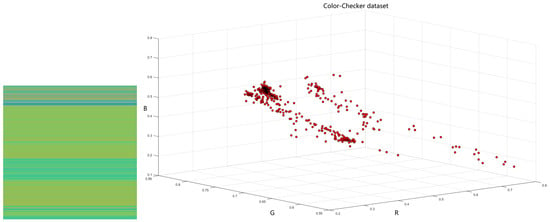
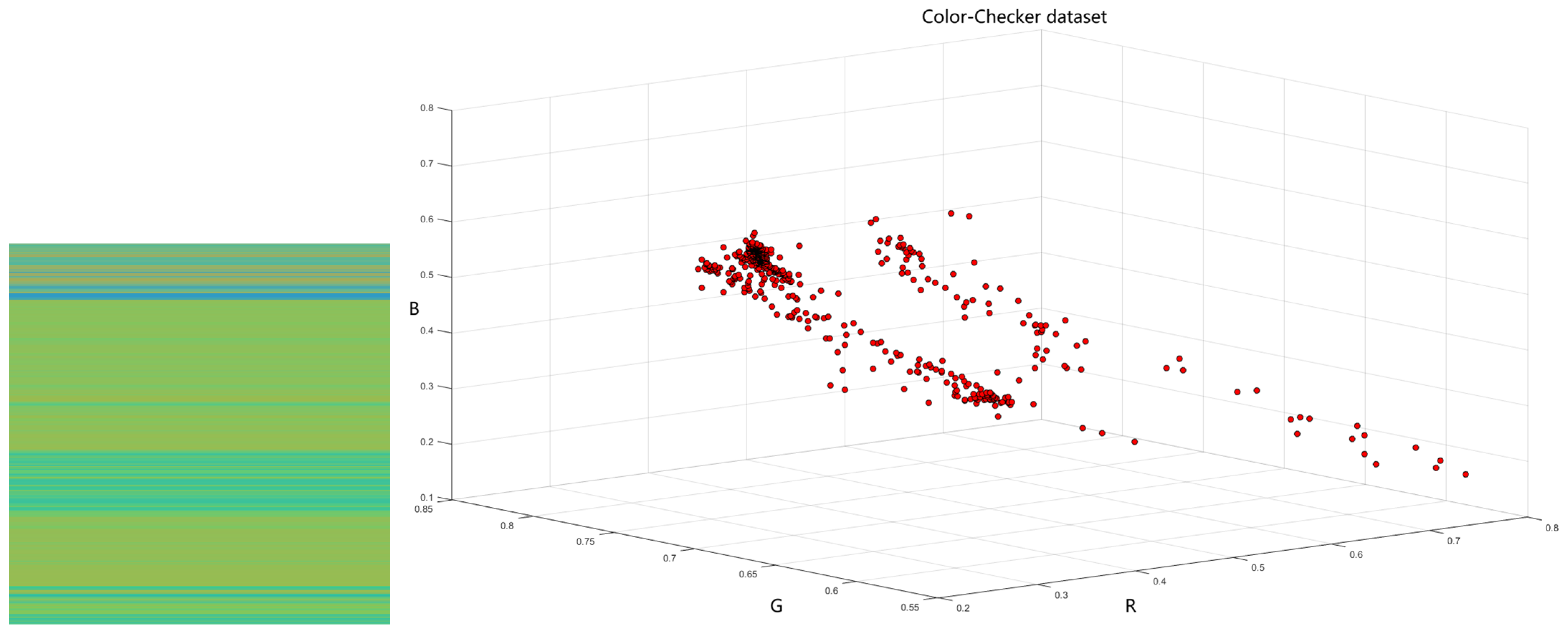
The Gehler dataset, consisting of 568 images, offers a range of indoor and outdoor scenes captured with two high-quality Digital Single-Lens Reflex cameras: the Canon 5D and the Canon 1D. Both cameras were set to auto mode for these shots. A notable difference between the two image sets is the black level setting: 129 for the Canon 5D and zero for the Canon 1D. However, the dataset size is insufficient for training a neural network. Moreover, the data labels lack broad distribution. Figure 1 shows that the predominant light color is green (on the left), and the labels of the Gehler dataset cluster into approximately five distinct groups (on the right), indicating limited informational depth in the labels.

Figure 1. The training label of the Gehler dataset.

The NUS dataset comprises 1736 images, subdivided into eight subsets, each containing approximately 200 images captured by a specific camera. Despite the substantial total number of images, the quantity of data within each NUS subset is less than that in the Gehler dataset. The Cube+ dataset, the most extensive in color constancy research, includes 1365 outdoor and 342 indoor images taken with a Canon 550D camera.

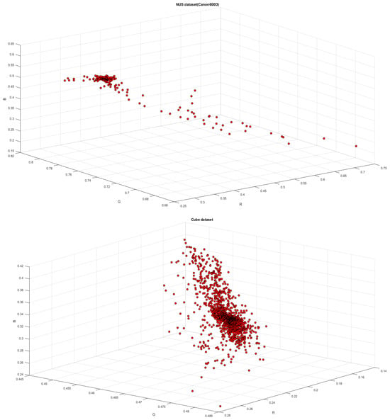
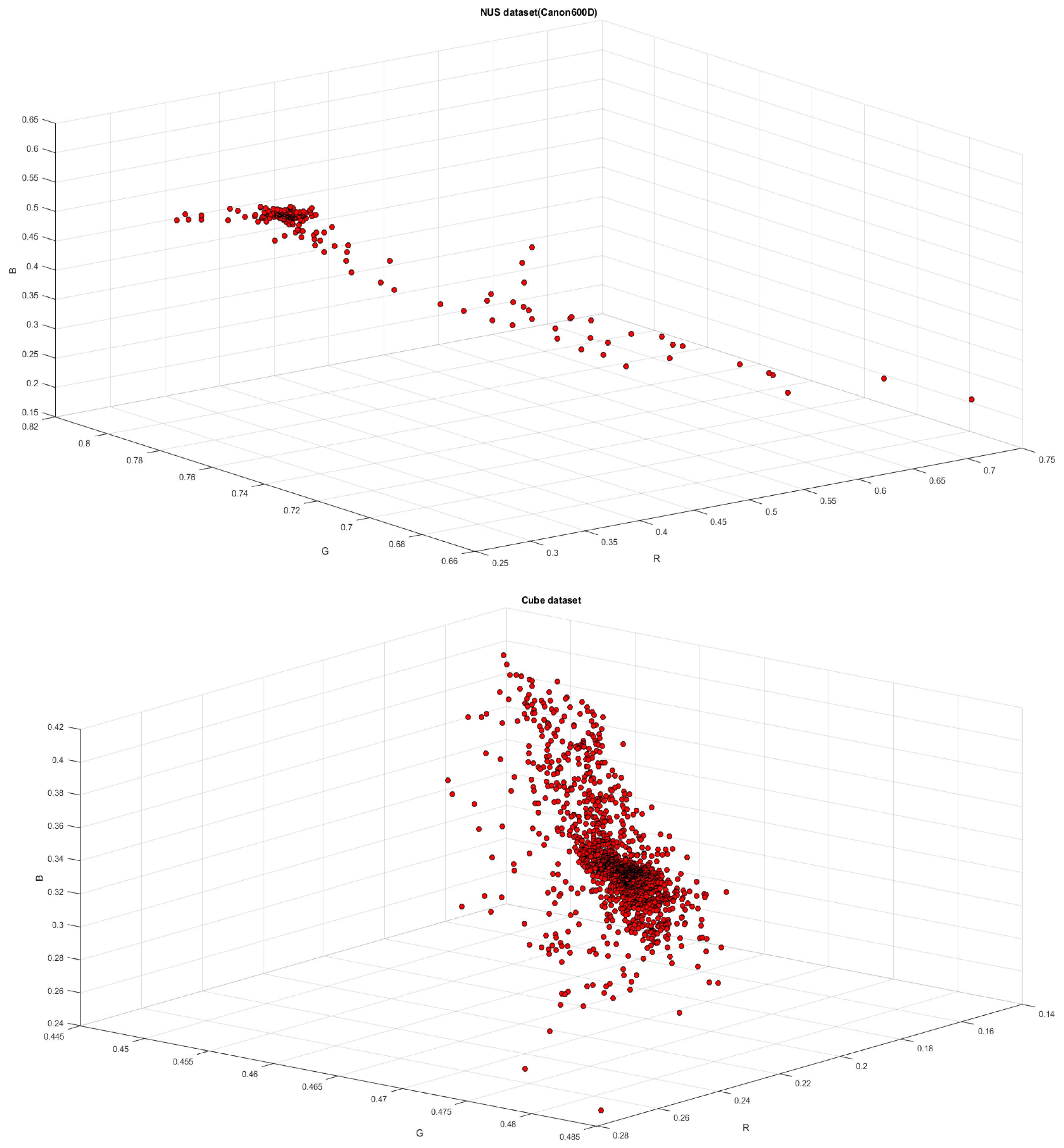
However, the label distribution in both the Gehler and NUS datasets is uneven, a characteristic that is not conducive to supervised learning. Figure 2 illustrates the illumination color of images captured by a Canon 600D camera in the NUS dataset (on the top). The labels within this subset form approximately one cluster. Similarly, the labels of the Cube+ dataset also coalesce into a single cluster with numerous isolated points (on the bottom of Figure 2). Consequently, the limited information contained in the labels of these two datasets may result in a diminished generalization capability of the network.

Figure 2. The training label of NUS and Cube datasets.

3.2. Output of Existing Models

Learning-based techniques use models learned from training data to estimate lighting colors, which typically have higher accuracy. The standard metrics used to estimate the results of lighting color experiments include mean, median, tri-mean of all the errors, mean of the lowest 25% of errors, and mean of the highest 25% of errors.

The experimental results from AlexNet (FC4) demonstrate that, when applied to the NUS 8-Camera dataset, the average error rate for the lowest 25% of predictions is 0.47, while the average error rate for the highest 25% of predictions is 5.15. Similarly, on the Color Checker dataset, the average error rate for the lowest 25% of predictions is 0.38, and for the highest 25%, it is 4.73. These results suggest that the model exhibits strong predictive performance. However, there is room for improvement in terms of its generalization capability and overall accuracy. This paper posits that the issue should be viewed in relation to the dataset rather than the neural network model.

4. Architecture of Piecewise Neural Network

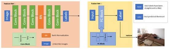
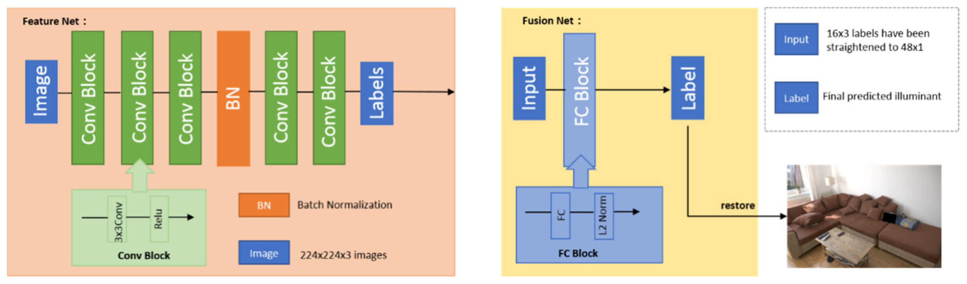
This network is comprised of two distinct entities: the feature network and fusion network. Every image within our expanded dataset is segmented into 16 partially overlapping blocks, all of which maintain the same label. This process effectively amplifies the dataset by a factor of 16. It is on this augmented dataset that the feature network undergoes its training process. The feature network comprises five convolutional layers, as depicted in Figure 3. The comprehensive structure of the network and its detailed parameters are provided in Table 1.

Figure 3. Architecture of the feature network and fusion network.

Table 1. Structure of the feature network. The chosen filter fully captures color information, eliminating the need for a complex neural network in recognition. Larger filters or more intricate structures were therefore not used.

Model	Input	Output
Layer 1	224 × 224 × 3	112 × 112 × 9
Layer 2	112 × 112 × 9	56 × 56 × 32
Layer 3	56 × 56 × 32	28 × 28 × 64
Batch normalization	28 × 28 × 64	28 × 28 × 64
Layer 4	28 × 28 × 64	14 × 14 × 64
Layer 5	14 × 14 × 64	7 × 7 × 3
Max pooling	7 × 7 × 3	1 × 1 × 3

Each convolutional block employs the ReLU activation function except for the final layer. The stride for each convolutional layer is set to 2. After the third layer, a batch normalization layer was introduced. In the last layer, we employed a max pooling operation using a 7 × 7 filter with zero padding to produce a 1 × 1 × 3 output, representing the illumination feature of a block within an image. The fusion network incorporates a single, fully connected layer. It accepts as input a 48-dimensional feature vector—an amalgamation of features derived from 16 distinct blocks within an image—and generates as output an estimation of the illumination color.

4.1. Feature Network

CNNs possess a robust learning capability, hence their extensive use in recent works on color constancy to learn features. We posit that the global convergence of convolutional neural networks is a prerequisite for their strong learning ability. The implementation of this global convergence hinges on three critical aspects: firstly, the network structure must be straightforward. Secondly, access to large datasets is imperative. Lastly, and most importantly, the data should possess a comprehensive information structure.

4.2. Fusion Network

In a strict sense, the fusion network is an adaptive weighted data fusion network designed to facilitate the complementation of output labels for various image blocks within an image. This approach distinguishes itself from others by ensuring system stability and robustness while diminishing reliance on feature networks. Essentially, the fusion network operates as a multiple linear regression model, enabling global estimations to align with the ground truth more closely.

5. Experiments

5.1. Data Augmentation and Preprocessing

Data augmentation is used to artificially increase the size of a dataset, typically by applying various transformations to the existing data. This process can significantly enhance the robustness and generalizability of machine learning models. In this study, we employ several augmentation methods to improve the performance of our model on the given dataset.

The initial step in data preprocessing involves cleaning and normalizing the raw data to ensure consistency and accuracy. We then split the dataset into training, validation, and testing sets, allowing for more efficient model training and evaluation. To further enhance the model performance, we apply techniques such as random rotation, flipping, and scaling to the images within the dataset. These augmented images serve as additional training examples, aiding the model in learning more complex and varied patterns present in the data.

In addition to image augmentation, we also perform text preprocessing for any accompanying datasets that include textual information. This involves tokenization, stop-word removal, and stemming or lemmatization to transform the text data into a more structured and meaningful format suitable for model training. Overall, through the combination of image and text preprocessing along with data augmentation, we aim to maximize the potential of our model by providing it with a diverse and comprehensive set of training data.

In research, frequently employed datasets encompass the NUS Dataset, ColorChecker Dataset, and the Cube Dataset. Nevertheless, as previously highlighted in Section 3, these datasets exhibit several shortcomings: notably, an insufficient number of images and a predominance of green images, which compromises their robustness. Given the typically small sizes of color constancy datasets, we propose a stochastic method for constructing training datasets based on the camera imaging pipeline, which has proven effective in practical applications. White-Balance is a component of the camera imaging pipeline and represents the linear processing of raw data, as shown in Figure 4.

Figure 4. The figure overviews the common steps applied onboard a camera.

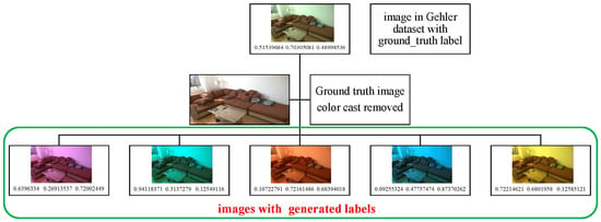
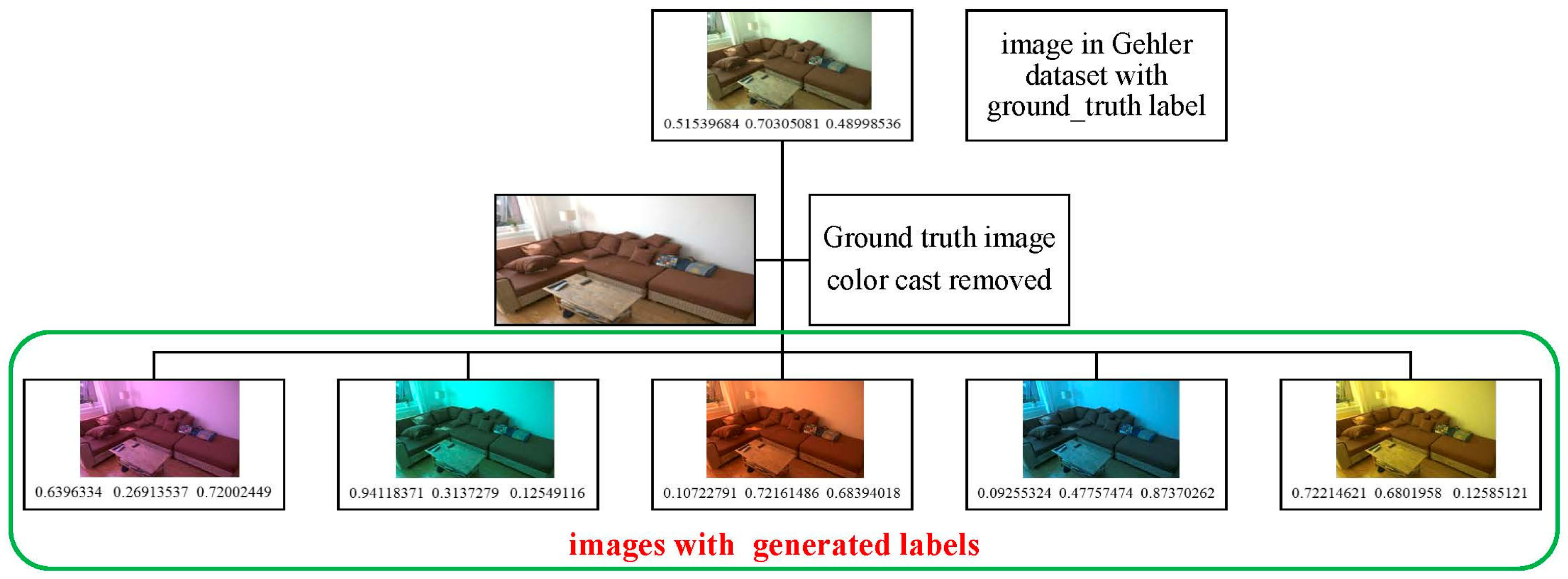
Initially, WB is adjusted for each digital image within the dataset using labels. Subsequently, five light labels (triples) are randomly generated for each image. These generated light labels are then incorporated into the white-balanced images to produce the novel database utilized in this study, as shown in Figure 5. This approach results in a five-fold expansion of the original dataset. Figure 6 provides an example of an image from the extended dataset.

Figure 5. The figure overviews the common steps to generate the new dataset.

Figure 6. The picture shows one example of an extended dataset.

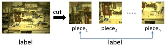
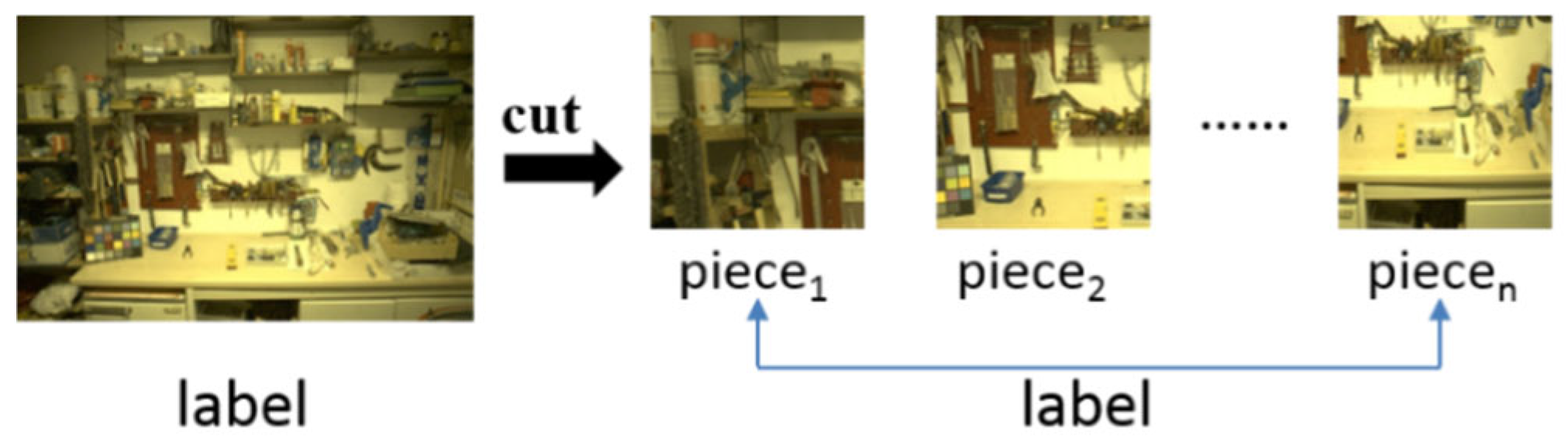
The corners of images influence subsequent network judgments, making it essential to transmit as much bottom-level information as possible. Many images, however, exhibit limited or muted color, which increases the risk of overfitting. To address this, the system must establish a robust color space by leveraging datasets with diverse color information, since a dull color space cannot adequately represent the richness of the real world. Conventional datasets are often restricted in this regard, leaving them vulnerable to incoherence in labeling and reduced robustness. To compensate, we remove the original colors from raw images, replace them with new random colors, and then segment these recolored images into repetitive pieces. These are fed into sample neural networks to construct a broader color space. Figure 7 shows the specific dataset processing method.

Figure 7. Randomly cut pictures ($2041\times 1359\times 3$) and cutting pieces ($224\times 224\times 3$) at the same color label.

5.2. Setting and Training

The neural network was implemented in TensorFlow 1.11 and trained by running 400,000 iterations of the Adam optimization algorithm. The loss function adopts the conventional error metric $F_{err}$ [15], and the learning rate of the network is $7\times {10}^{-4}$, with a batch size of 32.

$$F_{err}=\arccos \left({\displaystyle \frac{{{\displaystyle I}}_{es}{{\displaystyle I}}_{ori}}{‖{{\displaystyle I}}_{es}‖‖{{\displaystyle I}}_{ori}‖}}\right),$$

(3)

where ${{\displaystyle I}}_{ori}$ represents the real illuminant that we call label, and ${{\displaystyle I}}_{\mathrm{es}}$ represents the result of the network. We utilize the function to optimize the calculation of CNNs by reducing the error between the ground truth and our result.

New metrics can be used to optimize the algorithm and enhance results [10]. However, the simple error metric [Equation (3)] can be used to calculate better effects by randomly adding illumination to broaden the datasets. We used a three-fold cross-validation on the folds provided with the dataset: for each run, one is used for training (80%), one for validation (5%), and the remaining one for testing.

5.3. Comparison with Other Methods

In the study of color constancy, widely used datasets include the NUS Dataset, the Gehler–Shi Dataset, and the Cube Dataset. Our network was trained on the NUS and Gehler–Shi datasets, and we compared its performance with previous state-of-the-art methods on the same benchmarks. The results are presented in Table 2. Performance was evaluated using standard metrics, reported as angular error in degrees: mean, median, tri-mean, mean of the best 25%, and mean of the worst 25%.

Table 2. Angular error of algorithms, including the mean, median, and maximum value. The best results are indicated in bold.

Method		The Gehler–Shi Dataset						The NUS Dataset
		Mean	Median	Tricube Weight	Best 25%	Worst 25%	Average	Mean	Med.	Tricube Weight	Best 25%	Worst 25%	Average
Model driven	White patch [16]	7.55	5.68	6.35	1.45	16.12	5.76	10.62	10.58	10.49	1.86	19.45	8.43
	Gray world [17]	6.36	6.28	6.28	2.33	10.58	5.73	4.14	3.20	3.39	0.90	9.00	3.25
	1st-order Gray-Edge [18]	5.33	4.52	4.73	1.86	10.03	4.63	3.20	2.22	2.43	0.72	7.36	2.46
	2nd-order Grey-Edge [18]	5.13	4.44	4.62	2.11	9.26	4.60	3.20	2.26	2.44	0.75	7.27	2.49
	Shades-of-Grey [19]	4.93	4.01	4.23	1.14	10.20	3.96	3.40	2.57	2.73	0.77	7.41	2.67
	General Grey-World [20]	4.66	3.48	3.81	1.00	10.09	3.62	3.21	2.38	2.53	0.71	7.10	2.49
	Gray Index [21]	3.07	1.87	2.16	0.65	7.62	2.10	2.92	1.97	2.13	0.56	-	2.15
Data driven	Intersection-based Gamut [22]	4.20	2.39	2.93	0.61	10.70	2.76	7.20	5.96	6.28	2.20	13.61	6.05
	Edge-based Gamut [22]	6.52	5.04	5.43	1.90	13.58	5.40	8.43	7.05	7.37	2.41	16.08	7.01
	Pixel-based Gamut [22]	4.20	2.33	2.91	0.60	10.72	2.73	7.70	6.71	6.90	2.51	14.05	6.60
	Bayesian [2]	4.82	3.46	3.88	1.26	10.49	3.86	3.67	2.73	2.91	0.82	8.21	2.88
	Natural Image Statistics [23]	4.19	3.13	3.45	1.00	9.22	3.34	3.71	2.60	2.84	0.79	8.47	2.83
	Bright Pixels [24]	3.98	2.61	-	-	-	-	3.17	2.41	2.55	0.69	7.02	2.48
	Spatio-spectral (GenPrior) [25]	3.59	2.96	3.10	0.95	7.61	2.99	2.96	2.33	2.47	0.80	6.18	2.43
	Corrected-Moment [26]	2.86	2.04	2.22	0.83	6.34	2.25	2.95	2.05	2.16	0.59	6.89	2.21
	Regression Tree [27]	2.42	1.65	1.75	0.76	5.87	1.73	2.36	1.59	1.74	0.49	5.54	1.78
	CNN [7]	2.63	1.98	-	-	-	-	-	-	-	-	-	-
	CCC (dist+ext) [28]	1.95	1.22	1.38	0.62	5.07	1.40	2.38	1.48	1.69	0.45	5.85	1.74
	DS-net (HypNet+SelNet) [29]	1.90	1.12	1.33	0.53	5.81	1.34	2.24	1.46	1.68	0.48	6.08	1.74
	FC4 (AlexNet) [9]	1.77	1.11	1.29	0.60	4.29	1.30	2.12	1.53	1.67	0.48	4.78	1.66
	FFCC [30]	1.78	0.96	1.14	0.51	4.62	1.21	1.99	1.31	1.43	0.35	4.75	1.44
	Quasi-Unsupervised [31]	2.91	1.98	-	-	-	-	1.97	1.41	-	-	-	-
	Fast Color Constancy [31]	3.40	2.11	2.16	0.43	7.62	2.10	-	-	-	-	-	-
	DeepCC [32]	2.23	1.71	1.59	2.60	4.14	2.21	2.42	2.78	1.94	1.08	4.38	1.96
	Proposed	2.18	2.17	2.83	2.01	5.84	2.19	2.36	2.73	2.80	2.51	6.34	4.06

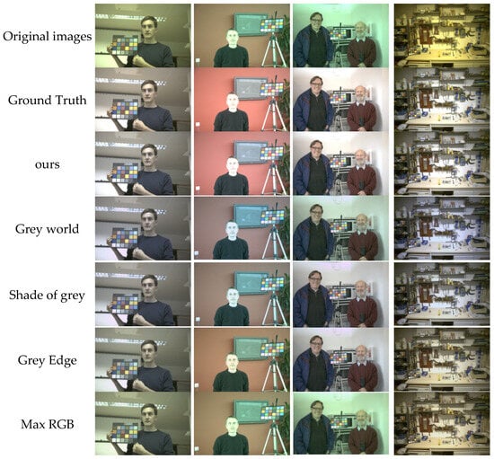
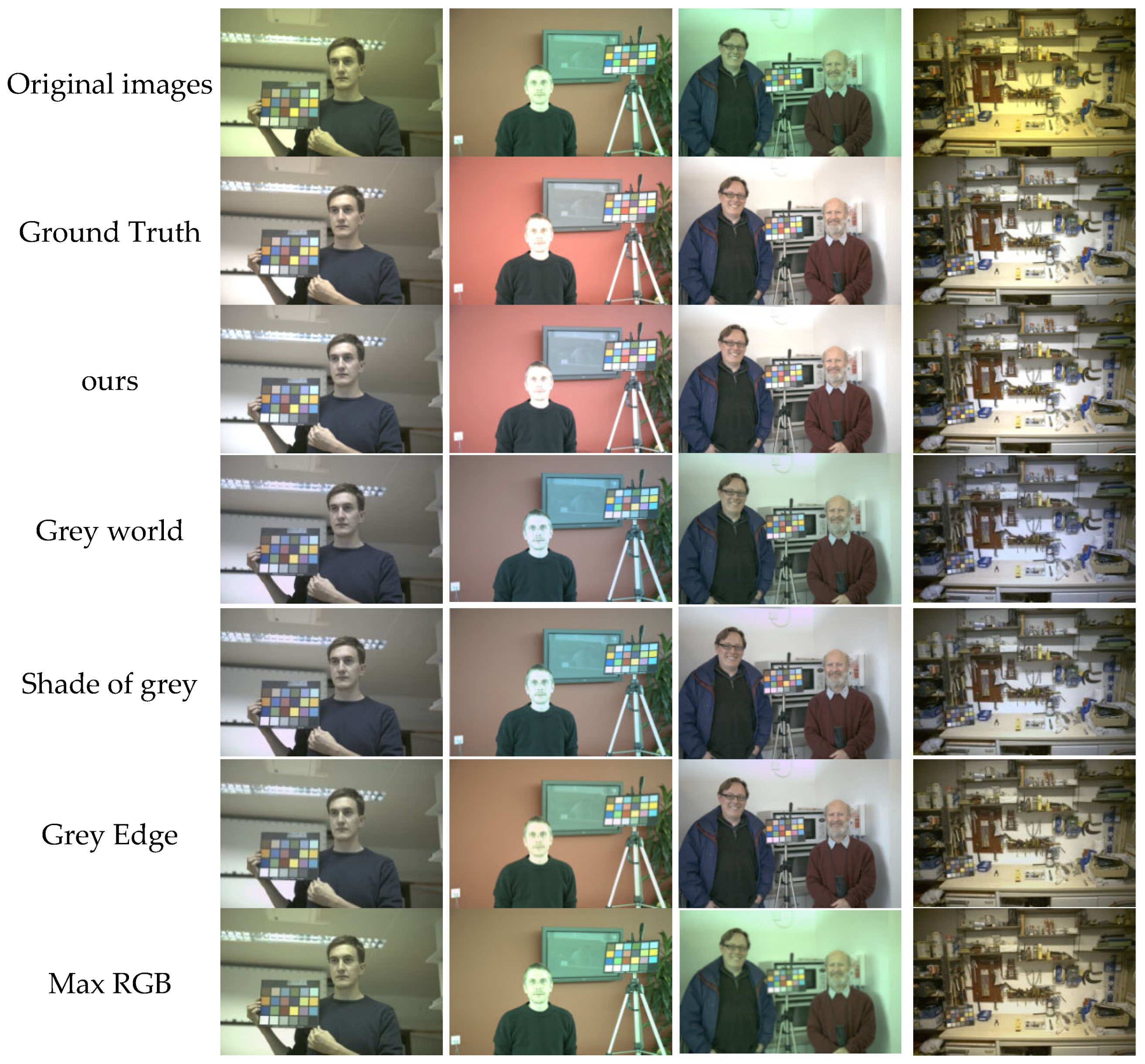
Testing outputs are presented in Figure 8, showing the input image, the images balanced according to the ground truth illuminant, and the images balanced according to the illuminant estimates.

Figure 8. Examples of datasets restored by our algorithm compared with conventional methods. The color checker remains in the images, as multiple light sources minimize its influence.

Table 2 and Figure 8 present the evaluation results of our supervised approach. Our method produces relatively small errors, with a maximum of 5.89, and achieves a lower average error than most existing algorithms. Performance is comparable to recent state-of-the-art methods such as FC4 and Quasi-U. Figure 8 illustrates several representative images, where we deliberately retained the Color Checker. We argue that all pixels contribute to overall color performance, and removing or masking the Color Checker could distort the extraction of global image information. Overall, our experimental results are strong, though some issues remain in brighter regions where fine-grained brightness adjustment is not fully resolved. Compared with leading methods, the developed approach in this study reduces mean error by 14% relative to FC4 and 20% relative to Dual-Stream Network (DS-NET). Median error is 31% lower than FC4, 30% lower than DS-NET, and 41% lower than Fast Fourier Color Constancy. Errors are more evenly distributed, with both maximum error reduced and overall variance controlled. While our dataset is somewhat limited and does not include additional benchmarks [27,28,29], we achieve improved results by modifying light source information.

6. Conclusions

The developed algorithm in this study achieves performance close to state-of-the-art networks. The cropped image strategy provides an effective way to expand training datasets, mitigating illumination incoherence and enhancing robustness. The network was trained on a mixture of the original Gehler dataset and processed images, with randomized input order to reduce overfitting. Data augmentation used heuristic values between 0.1 and 0.9, which lack precision for fully realistic illuminant simulation. This limitation can cause local brightening after white balance. Developing more accurate augmentation methods and extending beyond the assumption of a single global illuminant are key next steps. Recent work on multi-illuminant segmentation [33] suggests promising directions for adapting our piecewise network to complex, non-uniform lighting conditions.

References

- Karaimer, H.C.; Brown, M.S. A software platform for manipulating the camera imaging pipeline. In Proceedings of the Computer Vision—ECCV 2016: 14th European Conference, Amsterdam, The Netherlands, 11–14 October 2016. [Google Scholar]
- Gehler, P.V.; Rother, C.; Blake, A.; Minka, T.; Sharp, T. Bayesian color constancy revisited. In Proceedings of the 2008 IEEE Conference on Computer Vision and Pattern Recognition-CVPR 2008, Anchorage, AK, USA, 23–28 June 2008. [Google Scholar]
- Afifi, M.; Price, B.; Cohen, S.; Brown, M.S. When Color Constancy Goes Wrong: Correcting Improperly White-Balanced Images. In Proceedings of the 2019 IEEE/CVF Conference on Computer Vision and Pattern Recognition, Long Beach, CA, USA, 15–20 June 2019. [Google Scholar]
- Song, W.; Wang, Y.; Huang, D.; Liotta, A.; Perra, C. Enhancement of underwater images with statistical model of background light and optimization of transmission map. IEEE Trans. Broadcast. 2020, 66, 153–169. [Google Scholar] [CrossRef] [Scilit]
- Ruoteng, L.; Tan, R.T.; Cheong, L.-F. Robust optical flow estimation in rainy scenes. arXiv 2017, arXiv:1704.05239. [Google Scholar]
- Cheng, D.; Prasad, D.K.; Brown, M.S. Illuminant Estimation for Color Constancy: Why spatial domain methods work and the role of the color distribution. In Proceedings of the 2016 IEEE Conference on Computer Vision and Pattern Recognition-CVPR 2016, Las Vegas, NA, USA, 26 June–1 July 2016. [Google Scholar]
- Bianco, S.; Cusano, C.; Schettini, R. Color constancy using CNNs. In Proceedings of the 2015 IEEE Conference on Computer Vision and Pattern Recognition Workshops, Boston, MA, USA, 7–12 June 2015. [Google Scholar]
- Bianco, S.; Cusano, C. Quasi-Unsupervised Color Constancy. In Proceedings of the 2019 IEEE/CVF Conference on Computer Vision and Pattern Recognition, Long Beach, CA, USA, 15–20 June 2019. [Google Scholar]
- Hu, Y.; Wang, B.; Lin, S. FC4: Fully convolutional color constancy with confidence-weighted pooling. In Proceedings of the 2017 IEEE Conference on Computer Vision and Pattern Recognition-CVPR 2017, Honolulu, HI, USA, 21–26 July 2017. [Google Scholar]
- Das, P.; Baslamisli, A.S.; Liu, Y.; Karaoglu, S.; Gevers, T. Color Constancy by GANs: An Experimental Survey. arXiv 2018, arXiv:1812.03085. [Google Scholar]
- FiLaakom, F.; Passalis, N.; Raitoharju, J.; Nikkanen, J.; Tefas, A.; Iosifidis, A.; Gabbouj, M. Bag of color features for color constancy. IEEE Trans. Image Process. 2020, 29, 7722–7734. [Google Scholar] [CrossRef] [Scilit]
- Chen, C.; Chen, Q.; Xu, J.; Koltun, V. Learning to see in the dark. In Proceedings of the 2018 IEEE Conference on Computer Vision and Pattern Recognition-CVPR 2018, Salt Lake City, UT, USA, 18–22 June 2018. [Google Scholar]
- Li, B.; Qin, H.; Xiong, W. Ranking-based color constancy with limited training samples. IEEE Trans. Pattern Anal. Mach. Intell. 2023, 45, 12304–12320. [Google Scholar] [CrossRef] [Scilit] [PubMed]
- Hordley, S.; Finlayson, G. Re-evaluating color constancy algorithms. In Proceedings of the 17th International Conference on Pattern Recognition, Cambridge, UK, 23–26 August 2004. [Google Scholar]
- Afifi, M. Semantic WB: Semantic color constancy using convolutional neural network. arXiv 2018, arXiv:1802.00153. [Google Scholar]
- Brainard, D.H.; Wandell, B.A. Analysis of the retinex theory of color vision. JOSA A 1986, 3, 1651–1661. [Google Scholar] [CrossRef] [Scilit] [PubMed]
- Buchsbaum, G. A spatial processor model for object colour perception. J. Frankl. Inst. 1980, 310, 1–26. [Google Scholar] [CrossRef] [Scilit]
- Van De Weijer, J.; Gevers, T.; Gijsenij, A. Edge-based color constancy. IEEE Trans. Image Process. 2007, 16, 2207–2214. [Google Scholar] [CrossRef] [Scilit] [PubMed]
- Finlayson, G.D.; Trezzi, E. Shades of gray and colour constancy. In Proceedings of the 2004 Color and Imaging Conference-CIC 2024, Scottsdale, AZ, USA, 9–12 November 2004. [Google Scholar]
- Barnard, K.; Martin, L.; Coath, A.; Funt, B. A comparison of computational color constancy algorithms. ii. experiments with image data. IEEE Trans. Image Process. 2002, 11, 985–996. [Google Scholar] [CrossRef] [Scilit] [PubMed]
- Qian, Y.; Kamarainen, J.K.; Nikkanen, J.; Matas, J. On finding gray pixels. In Proceedings of the 2019 IEEE/CVF Conference on Computer Vision and Pattern Recognition, Long Beach, CA, USA, 16–20 June 2019. [Google Scholar]
- Barnard, K. Improvements to gamut mapping colour constancy algorithms. In Proceedings of the 6th European Conference on Computer Vision, Dublin, Ireland, 26 June–1 July 2000. [Google Scholar]
- Gijsenij, A.; Gevers, T. Color constancy using natural image statistics and scene semantics. IEEE Trans. Pattern Anal. Mach. Intell. 2010, 33, 687–698. [Google Scholar] [CrossRef] [Scilit] [PubMed]
- Joze, H.R.V.; Drew, M.S.; Finlayson, G.D.; Rey, P.A.T. The role of bright pixels in illumination estimation. In Proceedings of the 2012 Color and Imaging Conference-CIC 2012, Los Angeles, CA, USA, 12–16 November 2012. [Google Scholar]
- Chakrabarti, A.; Hirakawa, K.; Zickler, T. Color constancy with spatio-spectral statistics. IEEE Trans. Pattern Anal. Mach. Intell. 2011, 34, 1509–1519. [Google Scholar] [CrossRef] [Scilit] [PubMed]
- Finlayson, G.D. Corrected-moment illuminant estimation. In Proceedings of the 2013 IEEE International Conference on Computer Vision-ICCV 2013, Sydney, Australia, 1–8 December 2013. [Google Scholar]
- Finlayson, G.D.; Hordley, S.D. Color constancy at a pixel. JOSA A 2001, 18, 253–264. [Google Scholar] [CrossRef] [Scilit] [PubMed]
- Barron, J.T. Convolutional color constancy. In Proceedings of the 2015 IEEE International Conference on Computer Vision-ICCV 2015, Santiago, Chile, 13–16 December 2015. [Google Scholar]
- Shi, W.; Loy, C.C.; Tang, X. Deep specialized network for illuminant estimation. In Proceedings of the 21st ACM Conference on Computer and Communications Security, Scottsdale, AZ, USA, 3–7 November 2014. [Google Scholar]
- Barron, J.T.; Tsai, Y.-T. Fast fourier color constancy. In Proceedings of the 2017 IEEE Computer Vision and Pattern Recognition-CVPR 2017, Honolulu, HI, USA, 21–26 July 2017. [Google Scholar]
- Shi, Y.; Wang, J.; Xue, X. Fast color constancy with patch-wise bright pixels. arXiv 2019, arXiv:1911.07177. [Google Scholar]
- Flachot, A.; Akbarinia, A.; Schütt, H.H.; Fleming, R.W.; Wichmann, F.A.; Gegenfurtner, K.R. Deep neural models for color classification and color constancy. J. Vis. 2022, 22, 17. [Google Scholar] [CrossRef] [Scilit] [PubMed]
- Vršnak, D.; Domislović, I.; Subašić, M. Framework for illumination estimation and segmentation in multi-illuminant scenes. IEEE Access 2023, 11, 2128–2137. [Google Scholar] [CrossRef] [Scilit]
Disclaimer/Publisher’s Note: The statements, opinions and data contained in all publications are solely those of the individual author(s) and contributor(s) and not of MDPI and/or the editor(s). MDPI and/or the editor(s) disclaim responsibility for any injury to people or property resulting from any ideas, methods, instructions or products referred to in the content. |
© 2026 by the authors. Licensee MDPI, Basel, Switzerland. This article is an open access article distributed under the terms and conditions of the Creative Commons Attribution (CC BY) license.