Analysis and Comparison of Theoretical Estimates of the Material’s Cyclic Curve ^†

Abstract

Several formulations found in the literature allow estimation of the cyclic properties of materials based on static tensile test data, particularly for deriving the K′ and n′ parameters of the Ramberg–Osgood equation. This study assessed the consistency between the experimental cyclic stress–strain curves and those reconstructed using K′ and n′ values obtained by combining the various proposed relationships. The comparison was conducted using a dataset of 338 metallic alloys, predominantly iron-based, with additional aluminum and titanium alloys. As a comparison metric, the dimensionless deviation between the experimental and calculated curves was adopted. Statistical analysis of the results identified three combinations of relationships that yielded satisfactory agreement for 90% of the materials examined.

1. Introduction

The mechanical behaviour of a component is influenced by multiple factors, including its geometry, the material from which it is made, and the mechanical and chemical conditions it has experienced during manufacturing and service life. Consequently, a thorough understanding of material properties is essential for the effective design of any component. These properties are typically determined through experimental testing—some tests are straightforward and inexpensive, while others require significant time and resources. Among the more demanding procedures is the determination of the cyclic stress–strain curve, which plays a critical role in the design of components subjected to variable loading conditions and therefore susceptible to fatigue failure.

The cyclic stress–strain curve is typically obtained through experimental procedures such as the companion, incremental-step, and multiple-step test methods [1,2,3]. However, these techniques are often impractical during early design phases due to their complexity, cost, and time requirements. As an alternative, cyclic behavior can be inferred using compatibility relationships derived from the Basquin and Manson–Coffin equations. Yet, this indirect approach frequently yields results with limited accuracy [4,5]. To address these limitations, various researchers have explored statistical correlations based on extensive datasets of cyclic and monotonic tests accumulated over the years. This has led to the development of approximate formulas for estimating the parameters of cyclic stress–strain curves. The proposed methods span a wide range—from direct regression models based on monotonic properties [6,7,8,9,10], to indirect estimation techniques [11,12,13], and more advanced approaches such as neural networks [14,15] and genetic algorithms [16].

This study aims to assess the effectiveness of theoretical models available in the literature for estimating the cyclic stress–strain curve of metallic materials. The objective is to quantitatively evaluate the accuracy of these formulations and, by extension, their reliability for design applications. A statistical approach is adopted, using well-defined parameters to measure the degree of agreement between theoretical predictions and experimental data drawn from a comprehensive database of metallic alloys.

2. Metal Behaviour

In the domain of low-cycle fatigue, it is well established that when a material is subjected to alternating strain cycles of constant amplitude beyond its elastic limit, it initially undergoes either work hardening or softening. This transient phase continues until the material’s cyclic response stabilizes [17,18]. The cyclic curve is defined by connecting the peak points of the hysteresis loops generated under varying load amplitudes. As such, it characterizes the stabilized relationship between strain and stress amplitudes. Understanding the cyclic curve is essential for accurately assessing strain within the elastic–plastic regime. If design assumptions rely solely on static material properties, they may significantly underestimate the amplitude of plastic strain—in cases where cyclic softening occurs—leading to an overestimation of fatigue life.

The cyclic curve is typically represented analytically by the Ramberg–Osgood equation [19]:

$${\epsilon }_a={\displaystyle \frac{{\sigma }_a}{E}}+{\left({\displaystyle \frac{{\sigma }_a}{K^{\prime }}}\right)}^{{\displaystyle \frac{1}{{\displaystyle n^{\prime }}}}}$$

In addition to the modulus of elasticity, two other material-dependent parameters appear in this model: the cyclic hardening exponent n′ and the cyclic hardening coefficient K′. However, these values are rarely available in the literature, and, when required for accurate component design, must be determined experimentally using standardized specimens—significantly increasing costs.

The importance of knowing the two cyclic parameters—i.e., the material’s behaviour under fatigue loading—has led many researchers over the years to propose theoretical estimates for K′ and n′ based on more commonly performed experimental tests. Several relationships have been presented in the literature to evaluate these parameters using only data from monotonic tensile tests. Given the ease of access to tensile test data compared to cyclic data—which are not always available on specialized websites or in vendor catalogues—it is appropriate to assess the validity of these methods. The correspondence between experimental data and the coefficients obtained through these formulas has been evaluated quantitatively in an uncoupled manner, i.e., without considering their combined effect on the cyclic curve estimation. This final step has traditionally been carried out qualitatively, without defining a parameter to measure its effectiveness.

The aim of this work is to identify which combination of n′ and K′, estimated from existing literature formulas, best approximates the experimental cyclic curve. The objective is therefore to investigate the accuracy of these theoretical models and to quantitatively establish their reliability in evaluating the cyclic curve.

3. Materials and Methods

3.1. Brief Literature Review of Expression for the Cyclic Deformation Properties

Below is a concise overview of the theoretical formulations considered in this study for determining the coefficients K′ and n′. For further details, the reader is referred to the original publications. Formulations related to K′ are denoted by a number, while those for n′ are indicated by a letter.

In [20], Zhang Z. et al., based on an analysis of a database comprising 22 metallic materials—including steels, aluminium, and titanium alloys—proposed several correlations derived from a parameter introduced in the article, referred to as the “new fracture-ductility parameter” (α). This parameter is defined as the product of the true fracture strain (ε_f) and the reduction in area (ψ). The materials are classified into three groups:

• $\alpha <0.05 or 0.1\le \alpha <0.2$
• $0.05<\alpha <0.1$
• $\alpha >0.2$

The authors specify the most suitable formula for calculating the two parameters based on the previously defined material group. The required input data, in addition to the true fracture strain (ε_f) and the reduction in area (ψ), include the true fracture stress (σ_f), the yield strength (R_p), and the ultimate tensile strength (R_m), all expressed in MPa.

$$\left\{\begin{array}{c}{K^{\prime }=57\left({\sigma }_f\times {\epsilon }_f^{-n}\right)}^{0.545}-1220 for \alpha <0.05 or 0.1\le \alpha <0.2\\ {K^{\prime }=57\left({\displaystyle \frac{{\sigma }_f{R}_p}{R_m}}\times {\epsilon }_f^{-n}\right)}^{0.545}-1220 for 0.05<\alpha <0.1 or \alpha >0.2\end{array}\right.$$

(1)

$$\left\{\begin{array}{c}{n}^{\prime }=1.06n\left(1+\beta \left|1-{\displaystyle \frac{R_m}{R_p}}\right|\right) for \alpha <0.05 or 0.1\le \alpha <0.2\\ n^{\prime }=1.06n\left(1+\beta \left|1-{\displaystyle \frac{{\sigma }_f}{R_m}}\right|\right) for 0.05<\alpha <0.1\hfill \\ n^{\prime }={\displaystyle \frac{R_p\times n}{{\sigma }_f-R_m}} for \alpha >0.2\hfill \end{array}\right.$$

(A)

The two auxiliary coefficients n and β are calculated as follows:

$$\left\{\begin{array}{c}n={\displaystyle \frac{\log \left(\frac{{\sigma }_f^3\times R_m^2}{R_p^5}\right)}{3\log \left(500{\epsilon }_f\right)}} for \alpha <0.05 or 0.1\le \alpha <0.2\\ n={\displaystyle \frac{\log \left(\frac{{\sigma }_f^2}{R_p{R}_m}\right)}{2\log \left(500{\epsilon }_f\right)}} for 0.05<\alpha <0.1 or \alpha >0.2\end{array}\right.$$

$$\beta =\left\{\begin{array}{c}-1 if {\displaystyle \frac{{\sigma }_f}{R_p}}>1.6\\ 1 if {\displaystyle \frac{{\sigma }_f}{R_p}}<1.6\end{array}\right.$$

In [8], the authors present estimates for K′ and n′ based on a dataset of 57 steels. In some of these formulations, materials are categorized into two groups according to the R_m/R_p ratio. For the purposes of this study, only the formulations that require yield strength and tensile strength as input are considered, since other parameters—such as Brinell hardness, included in [8]—are not available in the database used for this work. The formulations, with R_m and R_p expressed in MPa, are as follows:

$$\left\{\begin{array}{c}{K}^{\prime }=1.16\left(R_m\right)+593 for {\displaystyle \frac{R_m}{R_p}}>1.2\\ K^{\prime }=3\times {10}^{-4}{\left(R_m\right)}^2+0.23\left(R_m\right)+619 for {\displaystyle \frac{R_m}{R_p}}\le 1.2\hfill \end{array}\right.$$

(2)

$$\left\{\begin{array}{c}{K}^{\prime }=1.15\left(R_p\right)+937 for {\displaystyle \frac{R_m}{R_p}}>1.2\\ K^{\prime }=3\times {10}^{-4}{\left(R_p\right)}^2+0.43\left(R_p\right)+514 for {\displaystyle \frac{R_m}{R_p}}\le 1.2\hfill \end{array}\right.$$

(3)

$$n^{\prime }=-0.33\left({\displaystyle \frac{R_p}{R_m}}\right)+0.40$$

(B)

$$\left\{\begin{array}{c}{n}^{\prime }=-0.37\log \left({\displaystyle \frac{0.75\left(R_p\right)+82}{0.16\left(R_m\right)+593}}\right) for {\displaystyle \frac{R_m}{R_p}}>1.2\hfill \\ n^{\prime }=-0.37\log \left({\displaystyle \frac{3\times {10}^{-4}{\left(R_p\right)}^2-0.15\left(R_p\right)+526}{3\times {10}^{-4}{\left(R_m\right)}^2+0.23\left(R_m\right)+619}}\right) for {\displaystyle \frac{R_m}{R_p}}\le 1.2\end{array}\right.$$

(C)

In [10], additional methods are proposed for estimating the cyclic curve parameters. These were developed using a database of 338 materials, including steels, aluminium, and titanium alloys. The materials are classified according to three distinct criteria. The first classification, used for calculating K′, separates materials based on the R_m/R_p ratio, as previously introduced, but with slightly different sampling:

• group A for ${\displaystyle \frac{R_m}{R_p}}\le 1.2$,
• group B for $1.2<{\displaystyle \frac{R_m}{R_p}}\le 1.4$,
• group C for ${\displaystyle \frac{R_m}{R_p}}>1.2$.

The second, used to calculate n′, is based on the parameter λ, linked to compliance with the assumption of volume conservation during the tensile test:

• group S for $\lambda \ge 0.01$,
• group T for $\lambda <0.01$,

with $\lambda =\left|{\epsilon }_f-ln\left({\displaystyle \frac{1}{1-\psi }}\right)\right|$. The third criterion separates materials based on their main alloying element:

• iron alloys,
• aluminium alloys,
• titanium alloys.

Three formulations for K′ are based on the same pair of equations consisting of a parabolic approximation and an exponential approximation; choosing one excludes the other.

$$\left\{\begin{array}{c}{K}^{\prime }=a{\left(R_p\times e^{{\displaystyle \frac{R_m}{R_p}}}\right)}^2+b\left(R_p\times e^{{\displaystyle \frac{R_m}{R_p}}}\right)+c\\ K^{\prime }=a{\left(R_p\times e^{{\displaystyle \frac{R_m}{R_p}}}\right)}^2\hfill \end{array}\right.$$

(4–6)

Depending on the material classification, different values are assigned to the constants a, b, and c, as listed in

Table 1. Numerical values of the constants in the various relations of reference [10].

Equation ID	Material	a	b	c
(4)	all	7.8907 × 10−5	0.10584	539.21
(5)	group A	0.94294	0.91662
	group B	1.8273 × 10−5	0.4769	153.75
	group C	9.6907 × 10−5	0.10348	502.7
(6)	group Fe	0.85122	0.94145
	group Al	0.34943	1.0508
	group Ti	2.5639	0.81372
(7)	all	0.36313	0.13482	−9.1678
(D)	all	0.62291	−0.10631	0.11462
(E)	group S	0.20111	0.20248	0.08914
	group T	0.7417	−0.17047	0.12603
(F)	group Fe	0.58241	−0.080276	0.11691
	group Al	0.85858	−0.42695	0.11592
	group Ti	−0.75383	0.57037	0.094639
(J)	group S	0.20111	0.20248	0.08914
	group T	−1.3789 × 10−4	−0.026021	0.025772
(G)	all	1.8205 × 10−4	0.019841	0.041905
(H)	group S	7.3684 × 10−4	0.011256	0.072551
	group T	−1.3789 × 10−4	−0.026021	0.025772
(I)	group Fe	−2.5002 × 10−3	0.023508	0.028644
	group Al	−6.0774 × 10−3	0.025446	0.063636
	group Ti	−1.1179 × 10−2	0.12176	−0.13029
(4) Fe	all	0.85122	0.94145
(5) Fe	group A	1.5219	0.85361
	group B	1.2091	0.90509
	group C	0.34545	1.064
(7) Fe	all	0.34893	0.14166	−16.549
(D) Fe	all	0.58241	−8.0276 × 10−2	0.11691
(E) Fe	group S	0.19505	0.20615	8.8753 × 10−2
	group T	0.56844	−4.9209 × 10−2	0.11994
(G) Fe	all	−2.5002 × 10−5	2.3508 × 10−2	2.8644 × 10−2
(H) Fe	group S	−7.4940 × 10−5	2.5522 × 10−2	2.0762 × 10−2
	group T	−1.3843 × 10−4	−2.5864 × 10−2	2.7568 × 10−2

. The appropriate formula is determined by the presence of the constant c: if c is provided, the parabolic form is used; otherwise, the exponential form applies. For the first two cases—as well as others discussed later—for improved accuracy with only iron alloys, the constants in Table 1 must be used with the suffix “Fe”.

An additional formula proposed in [10], applicable to the entire dataset, is expressed as follows:

$$K^{\prime }=0.36313\left(R_p\times e^{{\displaystyle \frac{R_m}{R_p}}}\right)+0.13482\left(R_m\times e^{{\displaystyle \frac{R_m}{R_p}}}\right)-9.1678$$

(7)

The coefficients to be used for Fe alloys are also shown in Table 1.

Regarding the estimation of n′, two distinct formulations are proposed in [10], differing in the variables required for their application. The first relies solely on the values of R_m and R_p, while the second also incorporates the parameters E and σ_f. The coefficients vary according to the material classifications provided in Table 1.

$$n^{\prime }=a{\left({\displaystyle \frac{R_m-R_p}{R_m}}\right)}^2+b\left({\displaystyle \frac{R_m-R_p}{R_m}}\right)+c$$

(D–F)

$$n^{\prime }=a{\left[\left({\displaystyle \frac{E}{{10}^5}}\times {\displaystyle \frac{R_m}{R_p}}\right)+{\displaystyle \frac{{\sigma }_f}{R_p}}\right]}^2+b\left[\left({\displaystyle \frac{E}{{10}^5}}\times {\displaystyle \frac{R_m}{R_p}}\right)+{\displaystyle \frac{{\sigma }_f}{R_p}}\right]+c$$

(G–I)

An additional proposed relationship is:

$$\left\{\begin{array}{c}{n}^{\prime }=0.20111{\left[\left({\displaystyle \frac{E}{{10}^5}}\times {\displaystyle \frac{R_m}{R_p}}\right)+{\displaystyle \frac{{\sigma }_f}{R_p}}\right]}^2+0.20248\left[\left({\displaystyle \frac{E}{{10}^5}}\times {\displaystyle \frac{R_m}{R_p}}\right)+{\displaystyle \frac{{\sigma }_f}{R_p}}\right]+8.9140\times {10}^{-2} group S\\ n^{\prime }=-1.3789\times {10}^{-4}{\left({\displaystyle \frac{R_m-R_p}{R_m}}\right)}^2-2.6021\times {10}^{-2}\left({\displaystyle \frac{R_m-R_p}{R_m}}\right)+2.5772\times {10}^{-2} group T\end{array}\right.$$

(J)

3.2. Prediction of Cyclic Behaviour from Tensile Properties

The aim of this study is to evaluate the agreement between the experimental cyclic curve and that predicted using K′ and n′ values derived from tensile parameters. By combining seven formulations for K′ with ten for n′, a total of 70 different evaluations of the cyclic curve are obtained. The comparison with the experimental curve is carried out using the database presented in [10], which includes 338 alloys—primarily iron alloys, along with aluminium and titanium alloys. The available data comprise the two cyclic parameters (K′ and n′), Young’s modulus, yield and ultimate tensile strengths, and fracture strain. For a smaller subset of materials, true fracture strain, true fracture stress, and reduction in area are also available.

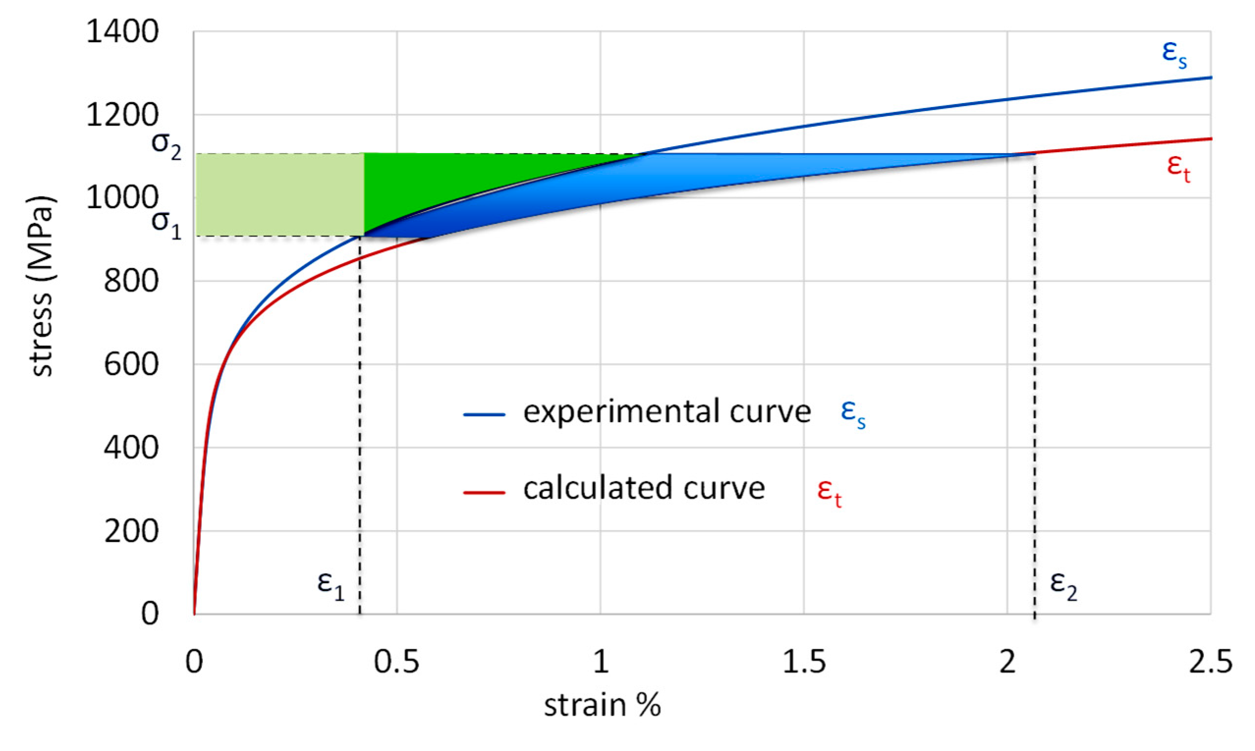
To compare the predicted and experimental curves, the difference in the area under the curves—expressed in terms of stress—between two defined stress values is used. To highlight deviations from experimental data, the interval between σ₁ = 1.1 × R_p and σ₂ = 0.9 × R_m is selected. This interval is broader than the typical application range of the cyclic curve.

Since this interval varies across materials, it is necessary to normalize the difference in area under the curves using an appropriate parameter. Two parameters were selected:

• The area under the experimental curve over the selected interval
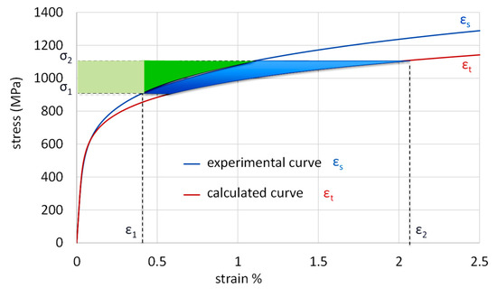
• The same area excluding the area under strain ε₁, where ε₁ is the strain corresponding to the σ₁ value of the experimental curve (Figure 1)
• The two variables chosen to evaluate the correspondence between the experimental curve and the calculated curve are expressed as:

$${\displaystyle \frac{\left|{\int }_{{\sigma }_1}^{{\sigma }_2}\left({\epsilon }_t-{\epsilon }_s\right)d\sigma \right|}{{\int }_{{\sigma }_1}^{{\sigma }_2}\left({\epsilon }_s\right)d\sigma }}={ER}_1$$

$${\displaystyle \frac{\left|{\int }_{{\sigma }_1}^{{\sigma }_2}\left({\epsilon }_t-{\epsilon }_s\right)d\sigma \right|}{{\int }_{{\sigma }_1}^{{\sigma }_2}{ϵ}_s-\left[{\epsilon }_1\left({\sigma }_2-{\sigma }_1\right)\right]d\sigma }}={ER}_2$$

4. Results

4.1. Analysis of the Entire Material Database

The ER₁ and ER₂ values were calculated for all combinations of theoretical K′ and n′ values, and for all materials in the database for which the required input parameters were available. Due to the absence of true stress and strain data at fracture, in some cases, the calculations could only be performed on a subset of the database, as indicated in

Table 2. Percentiles of ER₁ and ER₂ distributions for all equation associations.

Equation Combination	Number of Materials	ER1			ER2
		Percentile			Percentile
		75	80	90	75	80	90
1-A	102	2.6423	4.1771	76.609	6.8119	9.3509	109.28
1-B	102	3.1806	4.4196	29.385	6.4021	14.437	76.527
1-C	102	4.4882	6.2572	76.563	11.949	16.158	107.57
1-D	102	1.6212	2.3728	26.641	5.1800	12.754	75.786
1-E	102	1.6212	2.3728	26.641	4.5427	9.382	61.207
1-F	102	1.4022	2.7675	27.200	4.5427	9.3820	61.207
1-G	102	0.8231	0.8322	5.4137	3.4669	4.3750	16.322
1-H	94	0.8177	0.8306	142.17	4.0008	4.8331	315.88
1-I	102	0.8177	0.8306	142.17	4.3018	16.655	45.307
1-J	94	11.214	20.875	152.9	19.968	42.184	625.51
2-A	102	4.7775	6.0812	10.074	18.004	21.547	48.322
2-B	338	0.8698	1.2323	2.9890	2.2265	3.4038	9.9674
2-C	338	0.7226	0.7945	0.9125	1.6569	2.0059	3.2724
2-D	338	0.8682	1.4394	3.2500	2.3335	3.4047	12.021
2-E	146	2.3140	3.0697	5.3658	6.9297	9.0314	20.352
2-F	338	0.9301	1.5885	3.5965	2.3690	3.8215	12.729
2-G	127	0.7566	0.7753	0.8001	1.4934	1.7225	2.4387
2-H	94	0.7834	0.7884	0.8266	2.4272	3.1218	4.5330
2-I	127	0.7834	0.7884	0.8266	16.203	29.424	48.325
2-J	125	11.386	13.265	19.027	19.393	24.314	37.599
3-A	102	5.2188	6.4210	9.6036	16.450	22.029	35.636
3-B	338	0.9931	1.3267	2.6442	2.4191	3.4669	9.6918
3-C	338	0.7432	0.7901	0.9100	1.6081	1.9368	3.4548
3-D	338	1.0189	1.5936	3.6627	2.5868	3.9700	12.424
3-E	146	2.6257	3.3923	5.2775	6.6850	10.4298	17.858
3-F	338	1.0359	1.6441	3.7954	2.4527	4.1045	11.260
3-G	127	0.7478	0.7661	0.7947	1.4934	1.7668	2.4606
3-H	94	0.7854	0.7944	0.8274	2.5106	3.4052	5.0452
3-I	127	14.792	18.795	58.243	23.082	38.242	65.114
3-J	125	10.924	13.344	18.299	19.096	22.302	39.233
4-A	102	2.0088	2.1312	3.4537	5.7060	6.6545	12.588
4-B	338	0.8343	0.8775	1.4245	2.0873	2.6308	3.9938
4-C	338	1.2414	1.4792	2.9241	2.9383	3.4078	8.1723
4-D	338	0.6584	0.7431	0.8624	1.3724	1.7316	2.7982
4-E	146	0.8321	0.9311	1.4418	2.0284	2.4588	3.7727
4-F	338	0.6666	0.7196	0.8637	1.2148	1.5179	2.9120
4-G	127	0.7892	0.7950	0.8263	2.1960	2.4076	3.5089
4-H	94	0.7817	0.7855	0.8232	2.4166	3.1114	4.8487
4-I	127	4.0101	10.058	38.237	8.7618	23.373	49.797
4-J	125	11.928	16.045	22.684	24.552	27.443	48.569
5-A	102	2.3271	3.3216	4.0483	7.4003	9.9423	19.540
5-B	338	0.7897	0.8546	1.4561	1.8647	2.4172	4.4712
5-C	338	0.9633	1.3121	2.4912	2.5852	3.1198	6.7014
5-D	338	0.6851	0.7328	1.2648	1.2834	1.6509	3.6217
5-E	146	0.7436	0.8944	1.5965	2.0229	2.2448	5.6707
5-F	338	0.6604	0.7104	0.9802	1.1912	1.5791	3.3397
5-G	127	0.7845	0.7941	0.8204	2.1746	2.3335	3.4511
5-H	94	0.7819	0.7913	0.8262	2.3332	3.0864	4.8469
5-I	127	4.1233	8.0248	19.979	11.553	21.774	37.441
5-J	125	11.092	15.747	19.934	24.099	26.526	42.418
6-A	102	1.4826	1.8007	3.4529	5.1980	5.8267	10.667
6-B	338	1.0988	1.3341	3.0524	2.6089	3.2964	8.3038
6-C	338	1.7000	2.0724	5.0252	3.6071	4.3224	10.358
6-D	338	0.7533	0.8289	1.9262	1.7231	2.2540	6.5996
6-E	146	0.8780	1.1027	1.7855	2.2174	2.7917	5.6125
6-F	338	0.6916	0.7868	1.1274	1.4817	1.7943	3.3844
6-G	127	0.7898	0.7951	0.8275	2.1716	2.4116	3.5437
6-H	94	0.7817	0.7855	0.8232	2.3332	2.8787	4.8249
6-I	127	5.5288	8.7439	37.007	5.9255	11.846	4.2034
6-J	125	11.761	15.607	22.212	24.030	27.503	46.321
7-A	102	2.3272	2.8219	4.3602	6.5697	8.8693	18.351
7-B	338	1.0988	1.3341	3.0524	2.6089	3.2964	8.3038
7-C	338	1.5016	2.0124	4.1481	3.4923	4.2594	10.778
7-D	338	0.7650	0.8555	1.6857	1.6894	2.2403	5.8627
7-E	146	0.9002	1.2328	1.9639	2.5200	3.2665	6.6310
7-F	338	0.6754	0.7274	1.2829	1.2921	1.6088	4.8487
7-G	127	0.7875	0.7945	0.8255	2.1557	2.4012	3.4929
7-H	94	0.7819	0.7913	0.8232	2.3332	3.0868	4.8484
7-I	127	3.5342	4.9448	19.266	5.7103	11.905	46.529
7-J	125	10.849	15.829	23.031	22.913	26.833	43.195

.

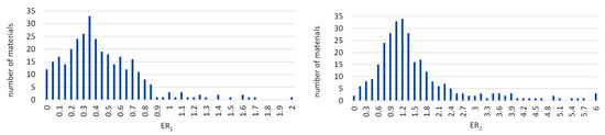
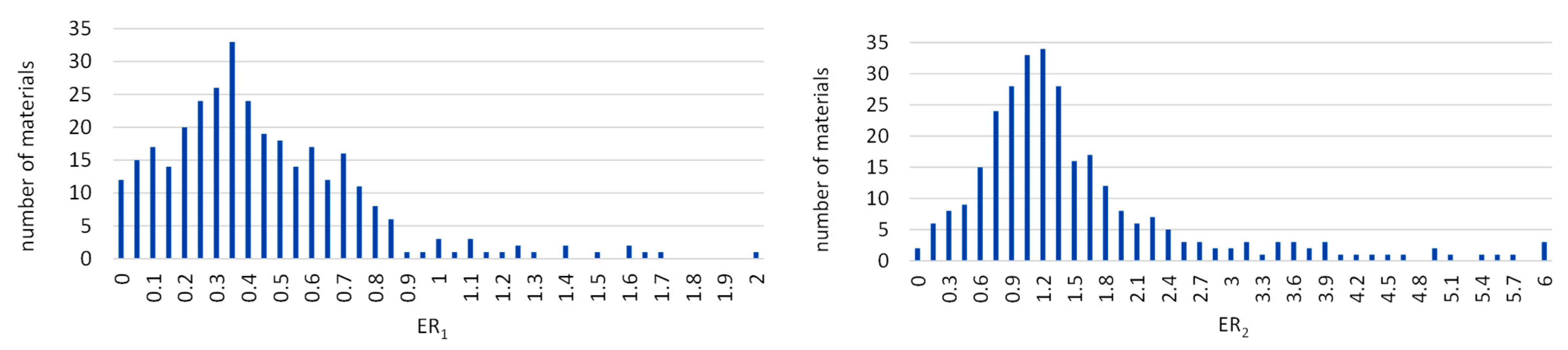
The ER₁ and ER₂ distributions exhibit a consistent trend across all cases: excluding a tail of high values—associated with a limited number of materials—the initial portion can be reasonably approximated by a Gaussian distribution. As an example, Figure 2 illustrates the two frequency distributions for combination 7-F.

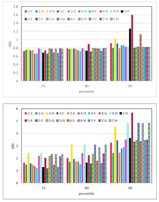
The best combinations were therefore identified based on percentile values, with particular attention to those beyond the third quartile, as shown in Table 2. An additional criterion was the number of materials for which the analysis could be performed. An initial selection was made by combining the top ten entries from each column in Table 2. The percentile distributions of these combinations are presented in Figure 3.

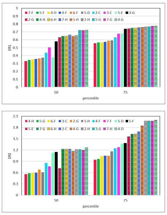
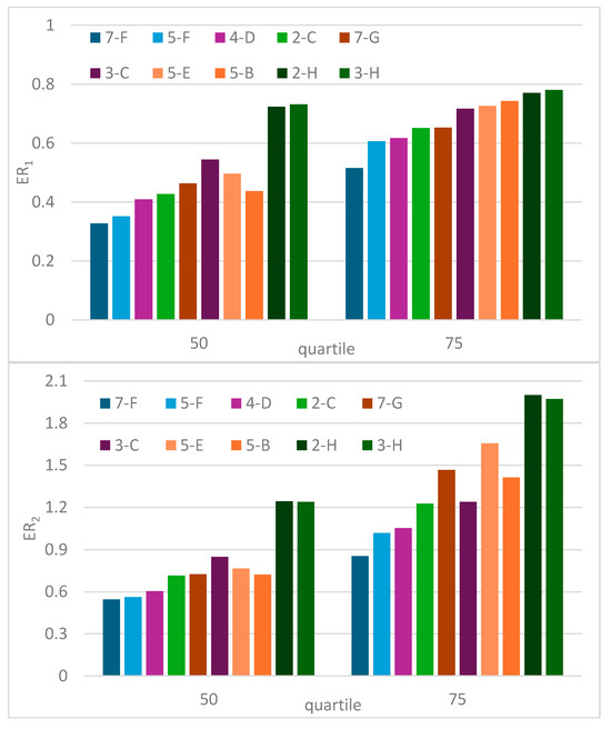
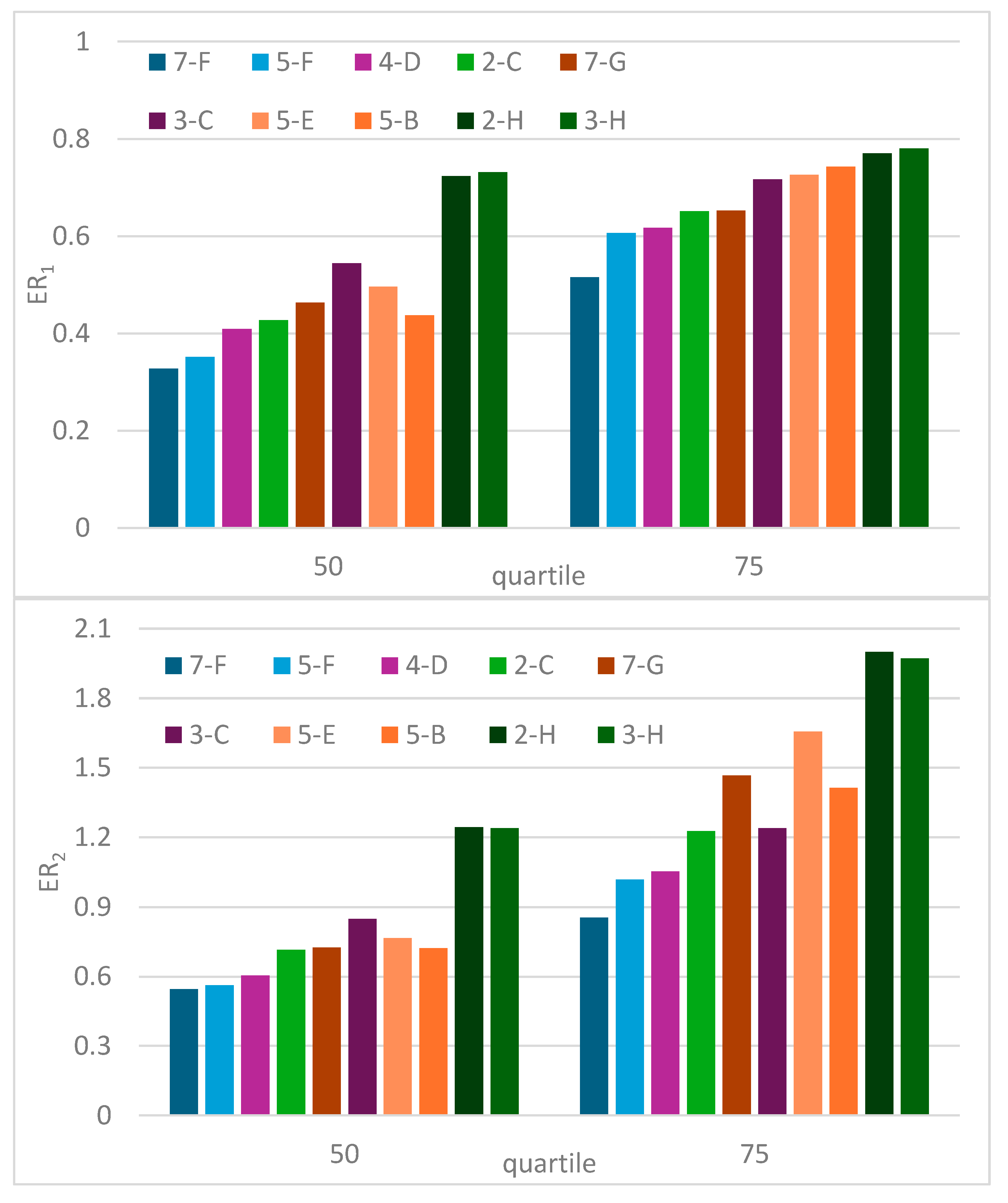
A further selection was made on the 90th percentile values. Combinations with ER₁ > 1 or ER₂ > 4 were excluded. To approach the ER1 and ER2 distributions closer to a behaviour that could be more accurately described by a Gaussian curve, new distributions were considered, derived from the previous ones by discarding values above the 90th percentile. This eliminates outliers associated with a small number of materials, which are not significant for the purposes of large-scale comparison. The two highest quartiles of these new refined distributions, relating to the combinations that passed the previous selections, are shown in Figure 4.

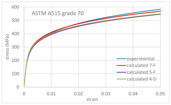
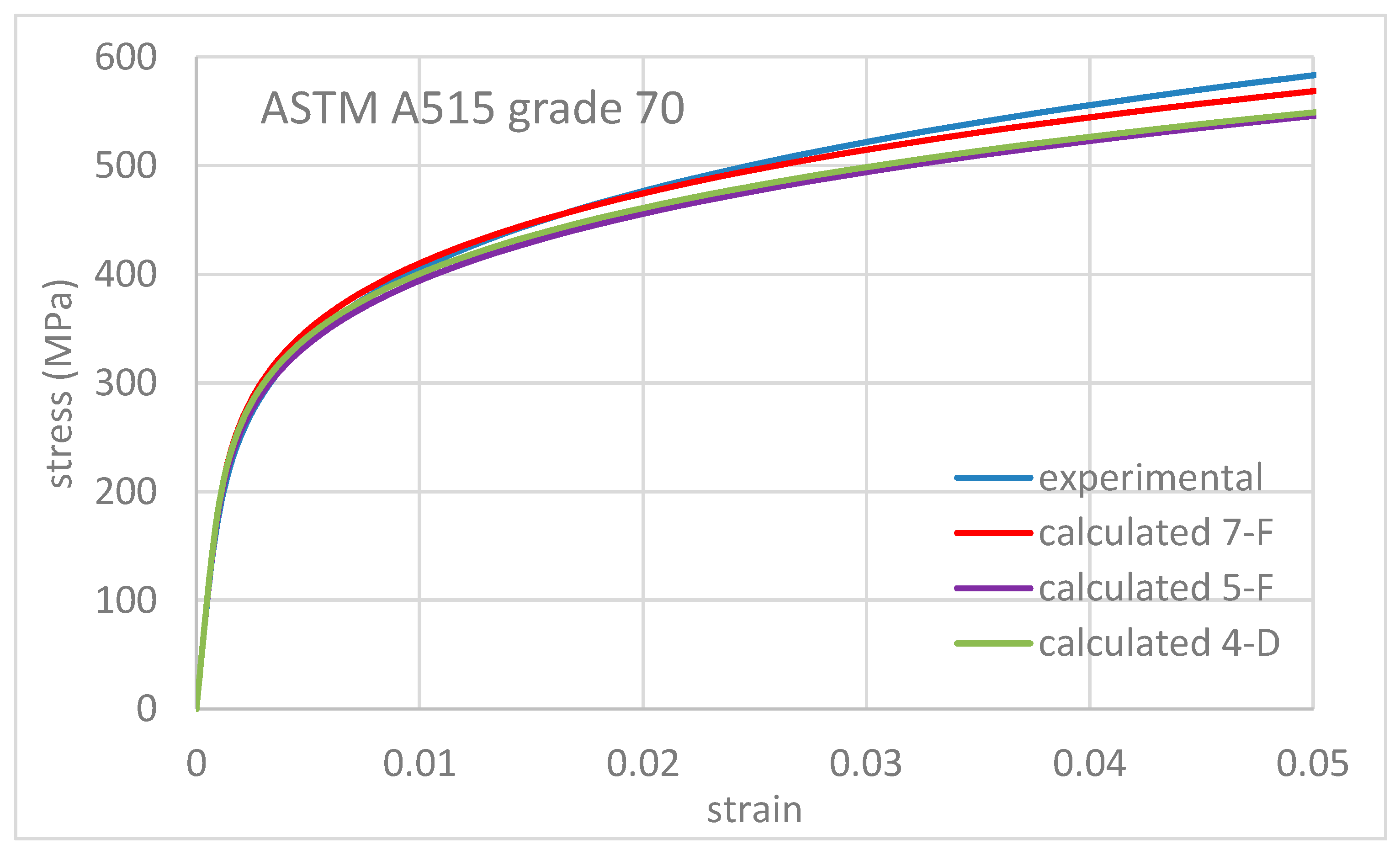
In both cases, the best-performing combination is 7-F, followed by 5-F, 4-D, and 4-F—all of which can be evaluated across the entire material database. Figure 5 presents a comparison between the experimental and calculated cyclic curves for the material whose ER₁ value corresponds to the median of the distribution.

For the four best combinations, an additional check was performed to determine whether the calculated curves overestimate, intersect, or underestimate the experimental curve within the selected interval. No dominant behavior was observed, as shown in

Table 3. Percentage of curves that overestimate, intersect, or underestimate the experimental curve.

Combination	Overestimation	Mixed	Underestimation
7-F	35.2%	19.5%	45.3%
5-F	33.4%	16.6%	50.0%
4-D	26.6%	24.9%	48.5%
4-F	29.6%	19.2%	51.2%

.

4.2. Analysis of Iron Alloys Only

The same analysis was repeated using a dataset limited to iron-based alloys. By excluding aluminium and titanium alloys, the number of applicable equation combinations was reduced to 53, as formulations independent of material classification overlapped with those specific to alloy type—for example, 2-D coincides with 2-F, and 4-D with 4-F. Since the procedure follows the same steps previously described, only the final results are shown in Figure 6. The top three combinations are the same as in the full dataset case. This is unsurprising, given that 86% of the database is composed of iron alloys.

5. Conclusions

The objective of this study was to identify the most accurate estimate of the cyclic curve using literature-based relationships for its coefficients. A statistical approach was applied to a comprehensive database of 338 metallic alloys, encompassing a wide range of chemical compositions and mechanical properties. The area enclosed between the calculated and experimental curves within a defined stress interval was normalized to derive two dimensionless comparison variables, which were used to evaluate the degree of agreement between the predicted and actual cyclic curves. Based on the percentile values of these variables, three sets of equations were identified that approximate the experimental curve with acceptable error for 90% of the materials. This result was confirmed even when the analysis was limited to iron-based alloys. Consequently, the cyclic curve can be reliably estimated using only the yield strength and ultimate tensile strength—parameters that are typically easy to obtain from the technical literature or supplier catalogs.

References

- Pickard, A.C.; Knott, G.F. Effect of Testing Method on Cyclic Hardening Behavior in Face-Centered-Cubic Alloys. In Low Cycle Fatigue ASTM STP 942; Solomon, H.D., Halford, G.R., Kaisand, L.R., Leis, B.N., Eds.; American Society for Testing Materials: Philadelphia, PA, USA, 1988; pp. 58–76. [Google Scholar]
- Jones, A.; Hudd, R.C. Cyclic Stress-Strain Curves Generated from Random Cyclic Strain Amplitude Tests. Int. J. Fatigue 1999, 21, 521–530. [Google Scholar] [CrossRef] [Scilit]
- Zonfrillo, G.; Nappini, D. Comparison of Procedures to Evaluate the Cyclic Stress-Strain Curve from Incremental Step Test. J. Mech. Eng. Autom. 2015, 5, 362–369. [Google Scholar] [CrossRef] [Scilit]
- Stephens, R.I.; Fatemi, A.; Stephens, R.R.; Fuchs, H.O. Metal Fatigue in Engineering, 2nd ed.; Wiley: New York, NY, USA, 2001. [Google Scholar]
- Meggiolaro, M.A.; Castro, J.T.P. A Critical Evaluation of Fatigue Crack Initiation Parameter Estimates. In Proceedings of the International Conference on Fatigue, São Paulo, Brazil, 21–23 June 2004. [Google Scholar]
- Zhang, Z.; Li, J.; Sun, Q.; Qiao, Y.; Li, C. Two Parameters Describing Cyclic Hardening/Softening Behaviors of Metallic Materials. J. Mater. Eng. Perform. 2009, 18, 237–244. [Google Scholar] [CrossRef] [Scilit]
- Basan, R.; Franulović, M.; Smokvina-Hanza, S. Estimation of cyclic Stress–Strain Curves for Low-Alloy Steel from Hardness. Metalurgija 2010, 49, 83–86. [Google Scholar]
- Lopez, Z.; Fatemi, A. A Method of Predicting Cyclic Stress–Strain Curve from Tensile Properties for Steels. Mater. Sci. Eng. A 2012, 556, 540–550. [Google Scholar] [CrossRef] [Scilit]
- Li, J.; Zhang, Z.; Li, C. An Improved Method for estimation of Ramberg–Osgood Curves of Steels from Monotonic Tensile Properties. Fatigue Fract. Engng. Mater. Struct. 2016, 39, 412–426. [Google Scholar] [CrossRef] [Scilit]
- Zonfrillo, G. New Correlations Between Monotonic and Cyclic Properties of Metallic Materials. J. Mater. Eng. Perform. 2017, 26, 1569–1580. [Google Scholar] [CrossRef] [Scilit]
- Basan, R.; Rubeša, D.; Franulović, M.; Križan, B. A Novel Approach to the estimation of strain life fatigue parameters. Procedia Eng. 2010, 2, 417–426. [Google Scholar] [CrossRef] [Scilit]
- Marohnić, T.; Basan, R.; Franulović, M. Evaluation of the Possibility of Estimating Cyclic Stress-Strain Parameters and Curves from Monotonic Properties of Steels. Procedia Eng. 2015, 101, 277–284. [Google Scholar] [CrossRef] [Scilit]
- Janežič, M.; Klemenc, J.; Fajdiga, M. A Neural-Network Approach to Describe the Scatter of Cyclic Stress–Strain Curves. Mater. Des. 2010, 31, 438–448. [Google Scholar] [CrossRef] [Scilit]
- Tomasella, A.; El Dsoki, C.; Hanselka, H.; Kaufmann, H. A Computational Estimation of Cyclic Material Properties Using Artificial Neural Networks. Procedia Eng. 2011, 10, 439–445. [Google Scholar] [CrossRef] [Scilit]
- Marohnić, T.; Basan, R.; Marković, E. Estimation of Cyclic Stress–Strain Curves of Steels Based on Monotonic Properties Using Artificial Neural Networks. Materials 2023, 16, 5010. [Google Scholar] [CrossRef] [Scilit]
- Franulović, M.; Basan, R.; Prebil, I. Genetic algorithm in material model parameters’ identification for low-cycle fatigue. Comput. Mater. Sci. 2009, 45, 505–510. [Google Scholar] [CrossRef] [Scilit]
- Dowling, N.E.; Kampe, S.L.; Milo, V. Mechanical Behavior of Materials, 5th ed.; Pearson: Harlow, UK, 2020. [Google Scholar]
- Paul, S.K. A Review on Cyclic Hardening and Softening Behavior of Alloys. J. Alloys Metall. Syst. 2025, 9, 100153. [Google Scholar] [CrossRef] [Scilit]
- Ramberg, W.; Osgood, W.R. Description of Stress–Strain Curves by Three Parameters; National Advisory Committee for Aeronautics: Washington, DC, USA, 1943. [Google Scholar]
- Zhang, Z.; Qiao, Y.; Sun, Q.; Li, C.; Li, J. Theoretical Estimation to the Cyclic Strength Coefficient and the Cyclic Strain-Hardening Exponent for Metallic Materials: Preliminary Study. J. Mater. Eng. Perform. 2009, 18, 245–254. [Google Scholar] [CrossRef] [Scilit]
Disclaimer/Publisher’s Note: The statements, opinions and data contained in all publications are solely those of the individual author(s) and contributor(s) and not of MDPI and/or the editor(s). MDPI and/or the editor(s) disclaim responsibility for any injury to people or property resulting from any ideas, methods, instructions or products referred to in the content. |
© 2026 by the authors. Licensee MDPI, Basel, Switzerland. This article is an open access article distributed under the terms and conditions of the Creative Commons Attribution (CC BY) license.