Experimentation of an Integrated Vision-Aided Inertial Navigation System with Orthophoto Matching on a Fixed-Wing UAV ^†

Abstract

This paper presents the work on integrating our Vision-Aided Inertial Navigation System (VaINS) with orthophoto matching to increase robustness to GNSS failure. Normalized cross-correlation is used to match onboard camera images with geo-referenced aerial imagery. Image sequences captured at a nadir angle by VaINS on a fixed-wing UAV are used in this experiment. The integrated navigation results are compared to both a smoothed GNSS-aided reference solution and the standalone VaINS solution during simulated GNSS-denied intervals. The results demonstrate that the integrated approach significantly outperforms the VaINS-only method. This is a preliminary investigation within ongoing work in orthophoto matching.

1. Introduction

Many unmanned aerial vehicles (UAVs) depend on Global Navigation Satellite System (GNSS) signals and inertial measurement units (IMUs) for accurate navigation. However, small UAVs with limited payloads often use low-performance IMUs, such that even brief GNSS outages lead to significant navigation errors due to high drift rates.

The Norwegian Defence Research Establishment (FFI) has been exploring an image-aided inertial navigation system [1] that integrates inertial sensor data with position data of image feature points across a sequence of images, using an error-state Extended Kalman Filter (EKF). A real-time navigation system called the Vision-Aided Inertial Navigation System (VaINS) was deployed and tested on a fixed-wing UAV [2] to collect data from multiple flights with varying camera pitch angles and were subsequently evaluated. Despite its increased performance, VaINS still experiences drift in error over time, necessitating a compensation mechanism. To address this, we propose an integrated navigation solution which combines visual–inertial odometry [1] and orthophoto matching that matches onboard images with geo-referenced aerial images (orthophotos).

The methods to address correspondence in geo-matching can generally be classified into the following three main categories: feature-point matching, template matching, and deep learning-based matching [3]. Feature-based matching involves extracting predefined features from both images and establishing correspondence based on these features. In contrast, template matching uses cross-correlation, applying a similarity measure to identify the best match between images. Deep learning-based matching integrates traditional computer vision techniques with neural networks.

Numerous methods [4,5,6,7,8,9] have been developed to match onboard camera images with geo-referenced imagery for aircraft positioning. Conte and Doherty [4] introduced a two-layer framework combining image alignment via normalized cross-correlation with inertial data integration. Grönwall et al. [5] enhanced this by incorporating lidar, while Patterson et al. [6] extended it using map features to improve 2D positioning.

Lindsten et al. [7] segmented camera and reference images into regions for matching. Cesetti et al. [8] applied scale-invariant feature transform (SIFT) feature matching, though their method required high-altitude operation. Chiue et al. [9] combined inertial data with 2D–3D tie points and geo-referenced feature tracks for image alignment and robust geo-referencing.

Orthophoto matching in the proposed navigation system employs normalized cross-correlation [10] (NCC), an area-based method, inspired by the work of Conte and Doherty [4], to align downward-facing onboard imagery with geo-referenced aerial images. Evaluating the position accuracy from NCC is challenging due to the lack of a universal algorithm for converting NCC into an accuracy measure. Conte and Dochery [4] state they use the NCC to compute the maximum likelihood, but do not show how. Tuna et al. [11] use the NCC directly as particle filter weights without specific arguments for this, while Vernaza and Lee [12] use a scaled NCC via a sigmoid function to generate a maximum likelihood for their Rao–Blackwellized particle filter update. However, Zucker [13] addressed this in 1D using a signal model linking NCC to maximum likelihood for radial velocity analysis. In this work, we extend Zucker’s approach to 2D and introduce a component to estimate the number of independent pixels for accuracy estimation.

This document describes orthophoto matching using NCC, integration of orthophoto matching with the INS, its performance in real data, and concludes the performance and presents the future works.

2. Orthophoto Matching

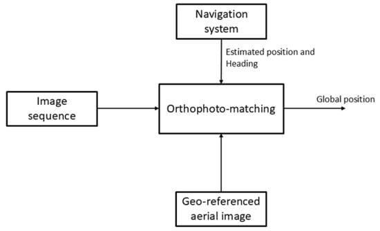
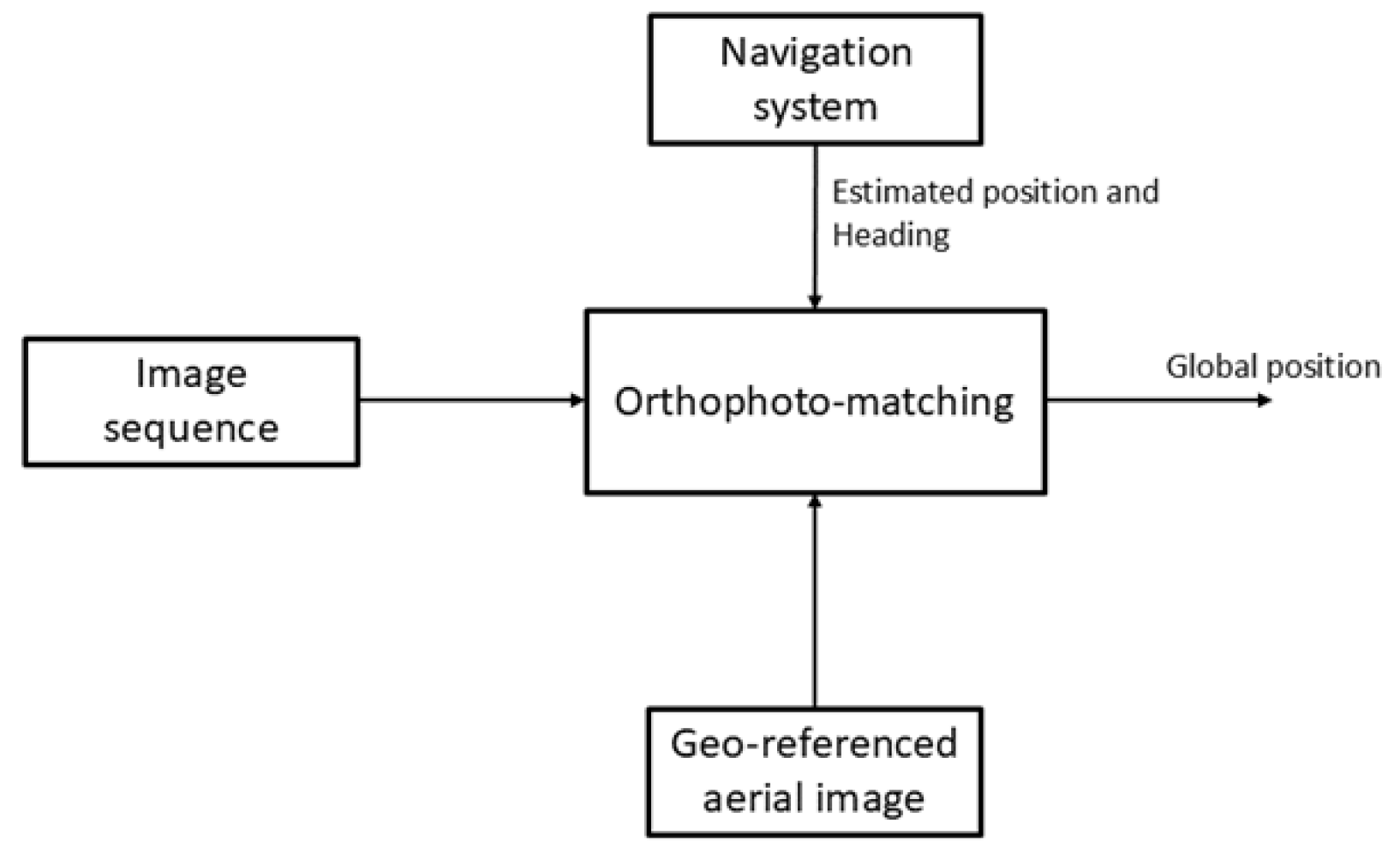
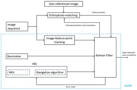
This section describes an algorithm that matches onboard camera images with orthophoto using normalized cross-correlation. Figure 1 shows the orthophoto-matching module, and the following subsections describe the algorithm in detail.

Figure 1. Orthophoto-matching module.

2.1. Initialization

Orthophoto matching requires a geo-reference image, the estimated navigation data from the INS, and the image sequence from the onboard camera system. The image timestamp is used to obtain the corresponding position and orientation from the estimated navigation solution. The onboard camera image is then rescaled to match the resolution of the orthophoto, referred to as the scaled camera image.

This study used image sequences captured at a nominal 90° pitch angle, but the aircraft’s orientation and camera misalignment caused the footprint deviation from the true nadir position. The corrected footprint is computed using aircraft attitude and camera misalignment. However, the terrain was assumed flat and orthorectification was avoided since we only considered periods of near-zero pitch and roll angles. To ensure that the scaled camera image fits after rotation, a region three times its size is cropped around the corrected footprint; then, it is rotated based on the estimated heading and the yaw misalignment angle of the camera. This is referred to as the rotated search region.

2.2. Template Matching

Template matching using the normalized cross-correlation (NCC) algorithm is performed between the scaled camera image and the rotated search region. Let $I(i,j)$ denote the scaled camera image and $R(i,j)$ the rotated search region image, then (1) expresses the NCC between I and R, where ${\mu }_I$ and ${\mu }_R$are the average pixel values of the I and the R, respectively.

$$NCC\left(u,v\right)={\displaystyle \frac{\sum _{i,j}\left[I\left(i,j\right)-{\mu }_I\right][R\left(i-u,j-v\right)-{\mu }_R]}{\sqrt{\sum _{i,j}{[I\left(i,j\right)-{\mu }_I]}^2}\sqrt{\sum _{i,j}{[R\left(i,j\right)-{\mu }_R]}^2}}}$$

(1)

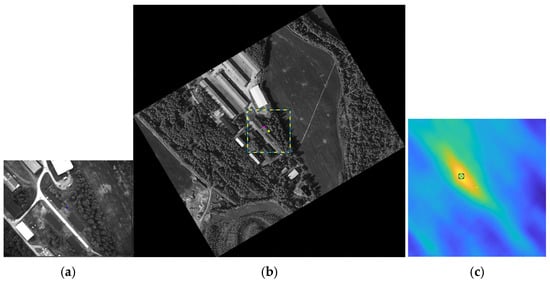
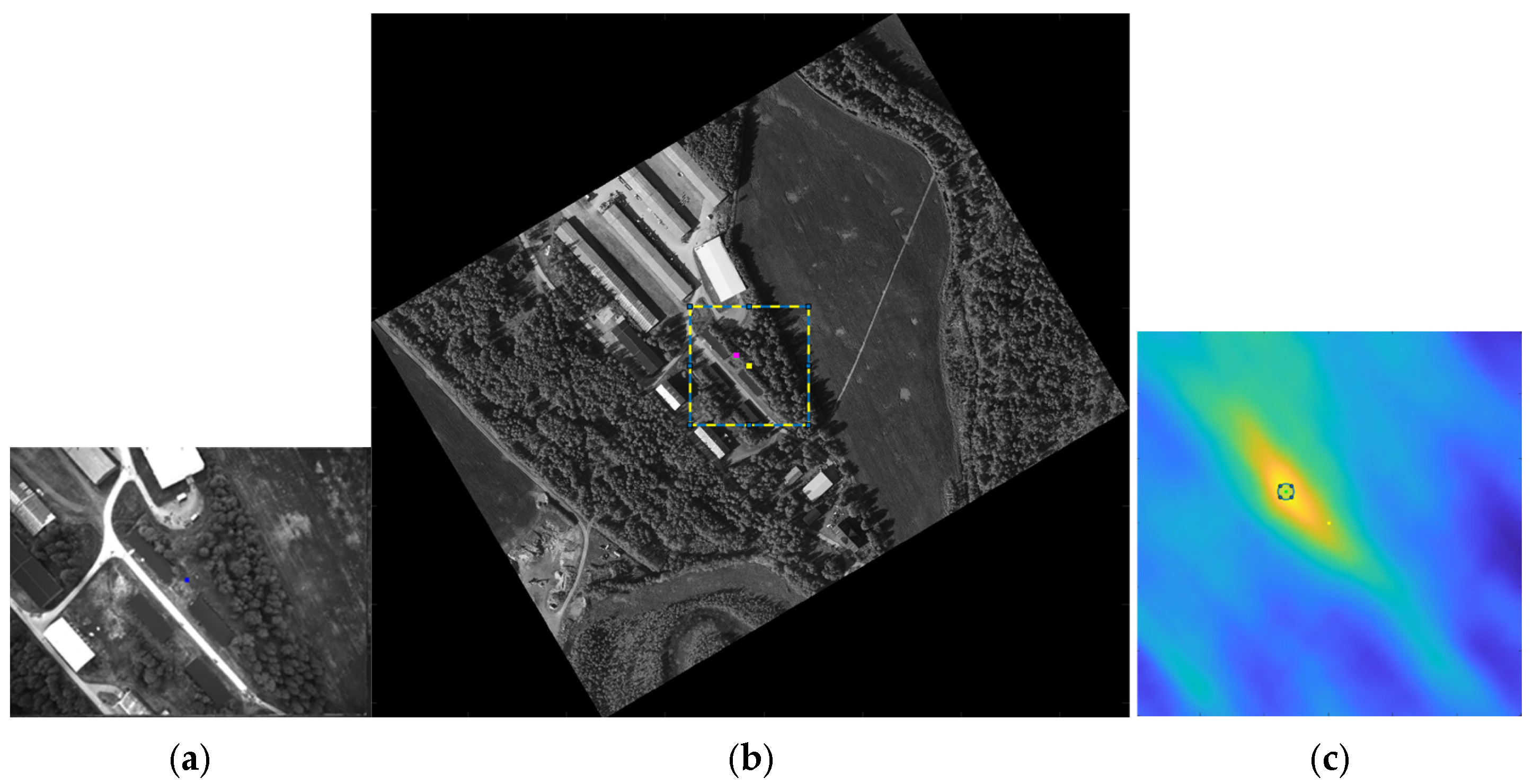
Firstly, NCC is performed within a predefined region around the center of the rotated search region to reduce computational time. The maximum NCC value (${NCC}_{max1}$), its position (${Max}_{pos1}$), and an uncertainty measure, named simplified ${NCC}_{\sigma },$ based on the dispersion of high NCC values are computed.

Figure 2 shows a scaled camera image (a), the corresponding rotated search region with predefined NCC computational region (b), and the corresponding NCC matrix (c).

Figure 2. (a) Scaled camera image. (b) Rotated search region with predefined NCC computational region. (c) NCC, where the center is marked yellow, its maximum value position is marked green, and the corresponding position in (b) is marked magenta.

If the ${NCC}_{max1}$ exceeds a predefined threshold, the simplified ${NCC}_{\sigma }$ is below a specified limit, and the ${Max}_{pos1}$ lies well within the matrix boundaries, the process proceeds to the next step. Otherwise, the matched position is rejected.

Then, the rotated search region is further rotated over a small range of angles around its initial orientation to account for the uncertainty in the yaw angle estimate from the INS. The NCC is then computed within a smaller region around the initial maximum position (${Max}_{pos1}$). The global maximum and its position ${(Max}_{pos2})$after the rotations are recorded. If ${Max}_{pos2}$ lies well within the matrix, it is accepted as the correct camera position, and the yaw angle is corrected accordingly. Otherwise, the process moves to the next step.

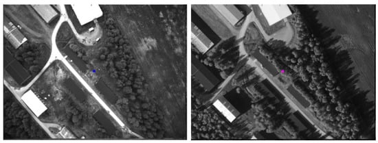
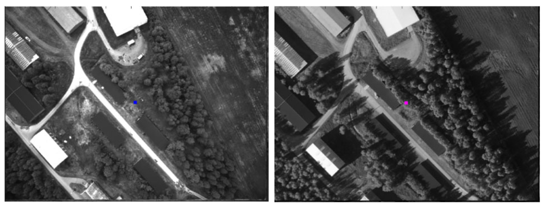
Finally, the rotated search region obtained after the second step is used to calculate the NCC within a larger region around ${ Max}_{pos2}$. If the new maximum NCC position (${Max}_{pos3}$) is located well within the matrix boundaries, it is accepted as the correct position; otherwise, it is discarded. The following figure, Figure 3, shows the camera image (left) and the region that matched its search region of orthophoto (right).

Figure 3. (Left) Camera image. (Right) Matched region in orthophoto.

3. Integration of Orthophoto Matching

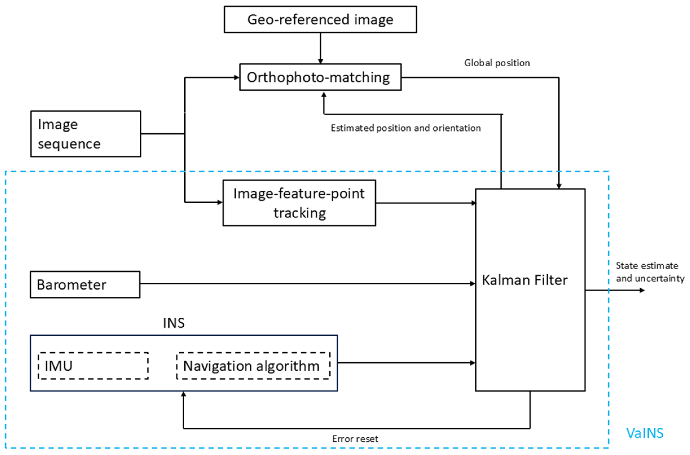
Figure 4 shows the integration of the orthophoto-matching module with VaINS by using the estimated position and orientation from VaINS as the initial parameter. The estimated position from orthophoto matching is sent to the EKF as a global position update, also requiring an estimate of its accuracy to be established for proper integration.

Figure 4. Integrated module of VaINS with orthophoto matching.

One option we looked at was to use the simplified ${NCC}_{\sigma }$ described in Section 2.2. Another is described in Section 3.1, where an accuracy estimate is presented by extending Zucker’s 1D algorithm to 2D using a simplified stochastic model for the image measurements. However, this model proved overconfident due to incorrect assumptions about pixel independence. To address this, Section 3.2 focuses on determining the actual number of effective pixels due to the actual dependency present.

3.1. Uncertainity from Zucker’s Algorithm in 2D

In [13] Zucker introduces a 1D stochastic signal spectrum measurement model that enables a connection between the NCC and its accuracy via Maximum Likelihood Estimation (MLE). The corresponding 2D model for image measurements is given by

$$I\left(x,y\right)=sR\left(x-\partial x,y-\partial y\right)+w\left(x,y\right),$$

(2)

where s is an unknown scalar, $(\partial x,\partial y)$ is the unknown translation, and $w$ is Gaussian white noise error with unknown scalar variance ${\sigma }^2$. By formulating the estimation of the translation as a MLE problem with (2) as model, and based on Zucker [13], we find the log measurement likelihood as

$$\log L(x,y)=-{\displaystyle \frac{n}{2}}\log \left(1-{NCC\left(x,y\right)}^2\right)+c,$$

(3)

where $c$ is a constant and $n$ is the number of pixels, here assumed to be independent. If all the model assumptions are correct, the MLE reaches the Cramer–Rao lower bound (CRLB) and we can use the CRLB covariance matrix as an estimate of the accuracy of the translation estimates found using NCC.

3.2. Number of Effective Pixels

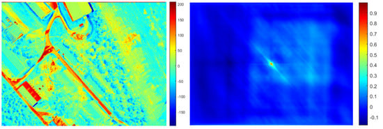
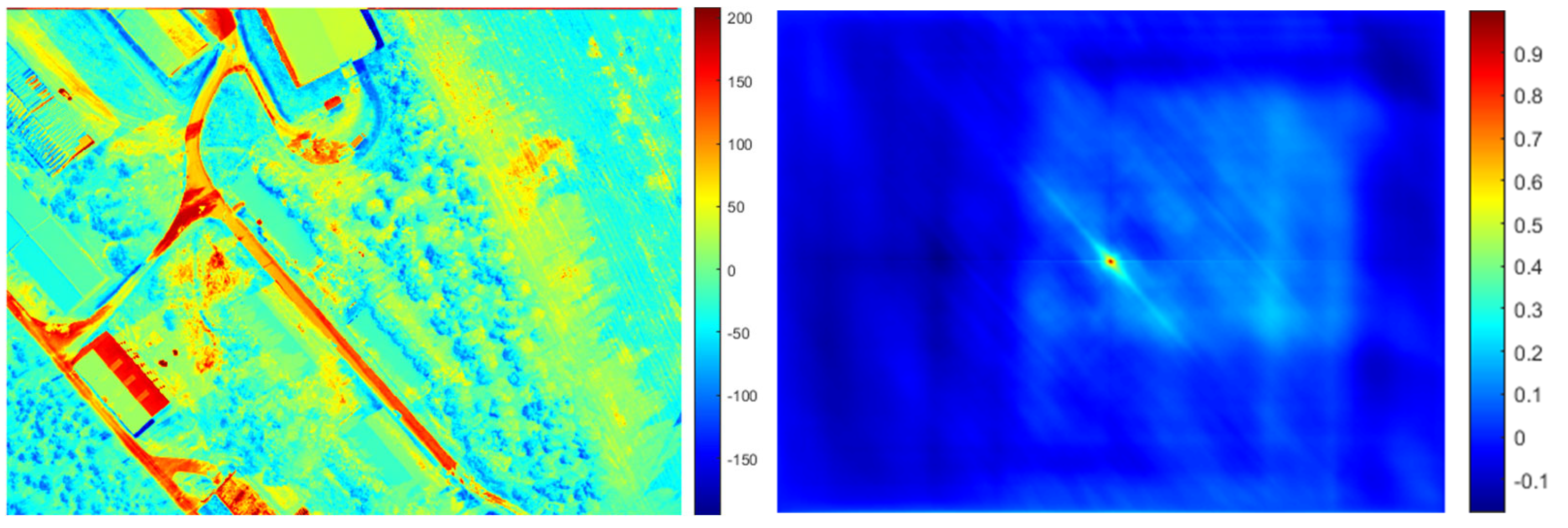
The estimated accuracy computed directly using the algorithm in Section 3.1 was found to be strongly overconfident. The main reason is that the pixel measurements in model (2) cannot be considered independent. In fact, there are a lot of reasons for expecting spatial correlations. Given that both $I$ and $R$ are images of an underlying scene that is not completely the same, we expect that neighbor pixels are correlated because of, e.g., different lighting situations, objects that are present in one image but not the other, man-made changes, or natural seasonal changes. To model this, we tried to estimate the number of effective pixels $n_{eff}$ that replace $n$ used in (3). Our approach is a generalization to 2D of the counting algorithm described for 1D sample sets in, e.g., [14]. First, we calculate the residual image from model (2) (see Figure 5 (left)) and then the normalized autocorrelation of this image shown in Figure 5 (right). Notice that anisotropic features in the residual image such as the roads break symmetry and are therefore also clearly visible in the normalized autocorrelation, as it is wider in the north-west/south-east direction. There are also signs of boundary effects, indicating that probably only the central part of the estimated normalized autocorrelation should be used, e.g., by using the first transit through zero as described in [15]. The normalized autocorrelation clearly indicates the presence of a high degree of spatial correlation. This normalized autocorrelation is then used as a measure of spatial correlation and as an input to a 2D version of the counting procedure in [14] that produces an estimate of $n_{eff}$.

Figure 5. (Left) Example of a residual image I-sR. (Right) The corresponding normalized autocorrelation of the residual image.

4. Experimental Setup

VaINS was used as a data-logging box on a fixed-wing UAV Scout in an earlier experiment [2]. It consists of three sensors and two processing units. The sensors are the MTi-100 MEMS IMU, a u-blox GPS, and an embedded Basler da1600 monochrome camera. The data were collected through five flights covering various parts of the landscape. For this study, only two datasets with pitch angle of 90° were used. The camera system in VaINS provided 8-bit monochromatic images with 10 Hz frame rate at a resolution of 1600 × 1200 pixels.

NavLab4, an updated version of the tool referenced in [16], was used to process and analyze the data in an offline setting. IMU and GPS data were processed using NavLab4’s optimal smoother to produce a reference dataset representing the aircraft’s position and orientation. This reference solution serves as the benchmark for evaluating both orthophoto matching and the integrated solution.

5. Performance

5.1. Orthophoto Matching

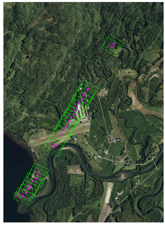
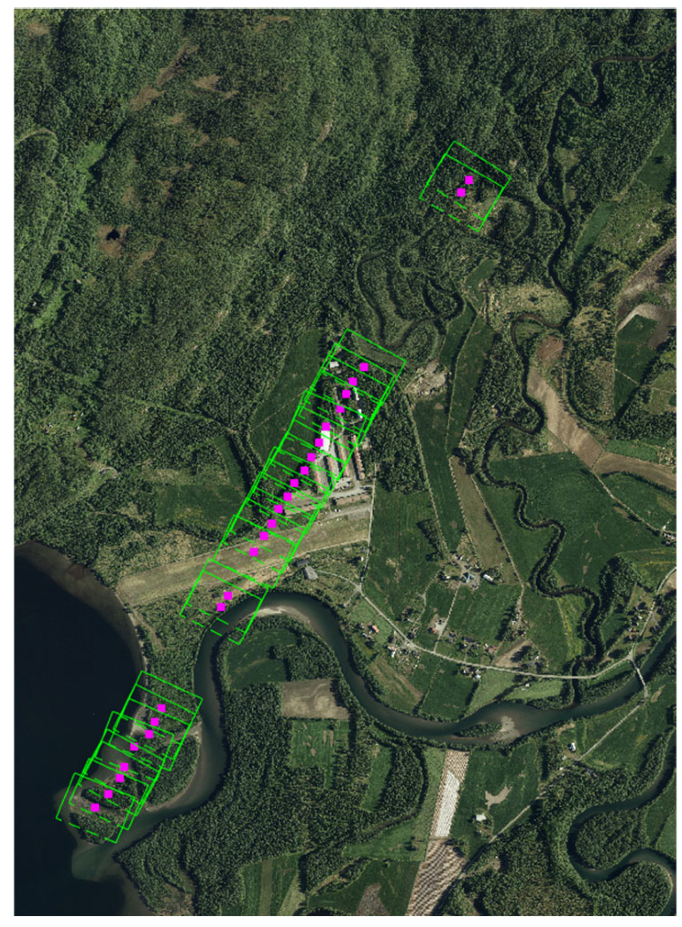
We observed that orthophoto matching performed quite effectively, particularly in the middle section of the flight where several man-made structures were present. Furthermore, it produced reasonable matches at the beginning and end of the flight, where no man-made structures were present. Figure 6 highlights the areas where orthophoto matching performed effectively.

Figure 6. Locations where NCC-based template matching was effective. The purple square marks the matched camera position; the green rectangle shows the image footprint.

A comparison of the normalized cross-correlation maximum values (${NCC}_{max}$) reveals that the values from the middle section are generally higher than those at the beginning and at the end.

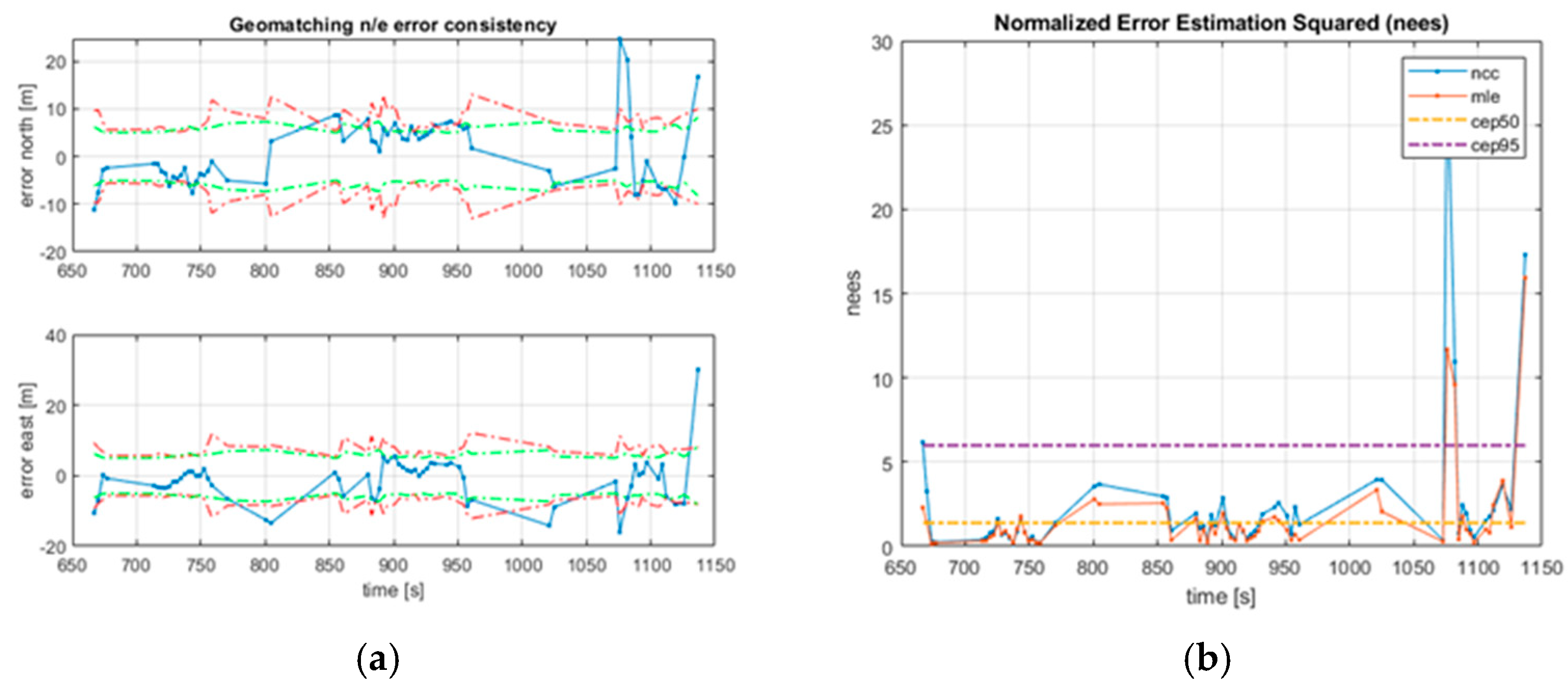
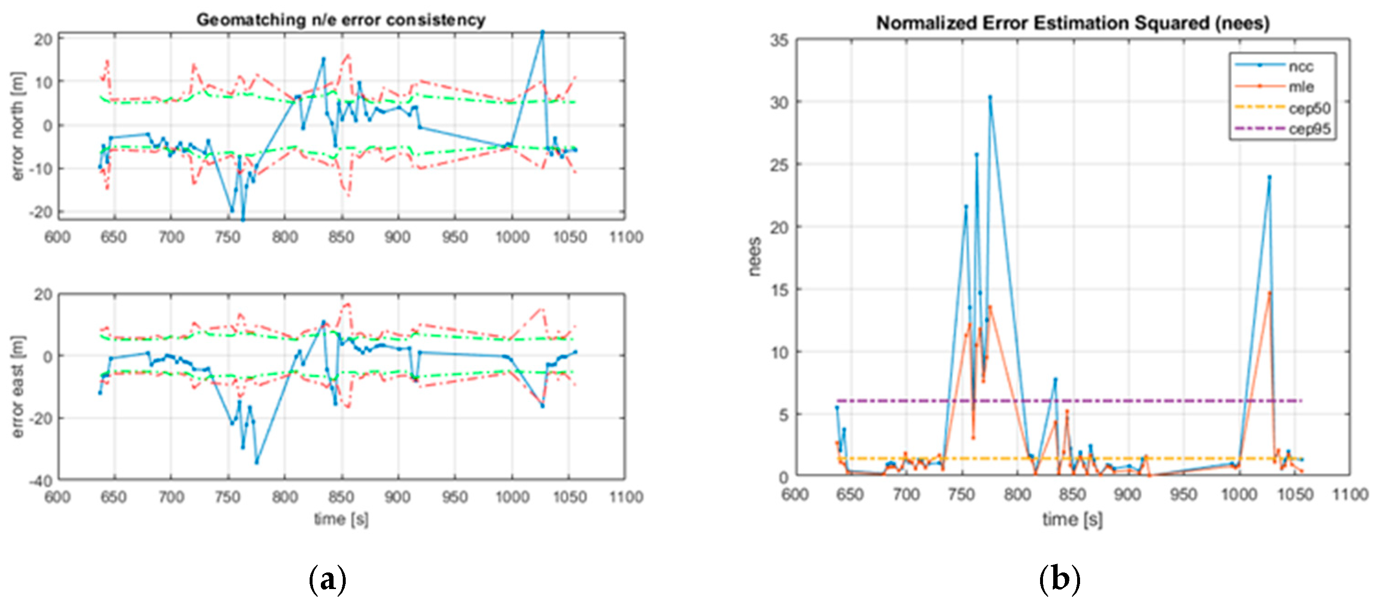
Figure 7 and Figure 8 show the position error plots comparing the reference and orthophoto matching during the GNSS-denied interval for the two datasets. The left side displays errors in the north and east directions, along with estimated uncertainties. The right side shows the Normalized Error Estimation Squared (NEES) and the 50% and 95% Circular Error Probabilities (CEP50, CEP95).

Figure 7. First dataset: (a) north and east error (blue) plotted with the estimated Zucker uncertainty (red) and the simplified ${NCC}_{\sigma }$ (green). (b) The corresponding NEES for Zucker (red) and NCC (blue) with the CEP50 and CEP95 confidence levels.

Figure 8. Second dataset: (a) north and east error (blue) plotted with the estimated Zucker uncertainty (red) and simplified ${NCC}_{\sigma }$(green). (b) The corresponding NEES for Zucker (red) and NCC (blue) with the CEP50 and CEP95 confidence levels.

For both datasets, the errors (left side) mostly stay within the estimated uncertainties. However, on the second flight (Figure 8), they exceed between 730 and 810 s and at the end of the flight. The NEES plots (right side) also remain within the CEP bounds most of the time but exceed even the upper bound during the same intervals. These discrepancies occur in areas where only vegetation and lakes are present.

5.2. Integrated Solution

The VaINS solution and the integrated orthophoto-matching solution are individually compared against the reference solution within the simulated GNSS-denied time intervals. Their performance is evaluated based on the root-mean-square (RMS) error between each solution and the reference solution.

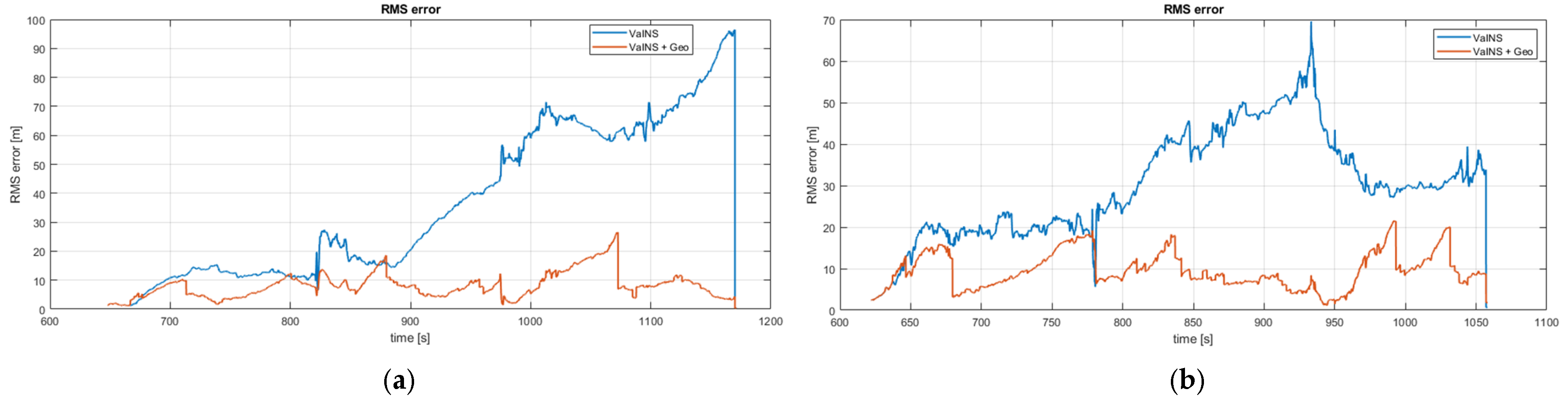
The following figure shows the RMS plot for the two datasets. The blue line shows the RMS of the VaINS solution, and the red line shows the RMS of the integrated solution. A comparison between the blue and red plots in Figure 9 highlights the performance improvement achieved by integrating orthophoto matching with the VaINS, particularly within the time interval of 824–1170 s. in the first dataset and 780–1057 s. in the second dataset. Figure 9 demonstrates that the error of the integrated solution remains within 26 m throughout the GNSS-denied interval in both datasets. However, the VaINS solution shows a higher error, remaining within 95 m for the first dataset and 70 m for the second dataset.

Figure 9. RMS error between the image-aided solutions and the reference solution for the two datasets: (a) first dataset and (b) second dataset. The RMS error of the VaINS solution is shown in blue, while the RMS error of the integrated solution is shown in red.

To further compare performance, additional statistics, the maximum RMS error during the GNSS-denied period (MaxE) and the RMS error at the end of that period (EndE)—are computed. Table 1 tabulates the GNSS-denied duration, flight distance, MaxE, and EndE for both datasets. The statistics for the VaINS solution (Va), the integrated solution (In), and the free inertial (Free) are reported separately.

Table 1. Statistics for both datasets: GPS-disabled duration, flight distance, maximum error (MaxE) within the duration, and the RMS error at the end of duration (EndE). “Va” denotes the VaINS solution, “In” denotes the integrated solution, and “Free” denotes the free inertial.

Data Set	Distance (m)	Duration (s)		MaxE (m)		EndE (m)
			Va	In	Va	In	Free
1	7136	550	95.9	26.4	95.7	4.3	8325
2	5976	435	69.6	21.3	33.8	8.8	2166

A comparison of MaxE values between the VaINS and integrated solutions reveals that the integrated solution reduces the MaxE by 72% in the first dataset and 69% in the second. Similarly, the EndE is reduced by 95% in the first dataset and 74% in the second. Comparing MaxE and EndE, the integrated solution outperformed the free-inertial.

6. Conclusions and Future Work

An integrated navigation system for GNSS-denied environments is presented, integrating a Vision-Aided Inertial Navigation System (VaINS) with orthophoto matching, and tested using two nadir-view image sequences captured by a fixed-wing UAV.

The VaINS solution and the integrated solution were then individually compared against the reference solution during a simulated GNSS-denied time interval. The integrated solution reduced the maximum RMS position error by approximately 70%, compared to VaINS solution, and maintained a bounded position error of less than 26 m throughout the GNSS-denied time intervals.

This study serves as a preliminary investigation into orthophoto matching, with a limited scope. Future work could expand this by testing various similarity measures for template matching to determine the most effective approach. Other methods for evaluating accuracy from the NCC could also be investigated further. With measurement likelihood computed from the NCC surface, future work can also focus on implementing an estimator to fuse matching results from multiple consecutive sequential images.

As an alternative to current orthophoto matching, matching could be performed by comparing current flight images with geo-referenced images from a previous flight or from earlier passes within the same flight.

References

- Baheerathan, S.; Hagen, O.K. Image-aided inertial navigation for an Octocopter. In Proceedings of the SPIE. Defense + Security 2018, Orlando, FL, USA, 15–19 April 2018. [Google Scholar]
- Baheerathan, S.; Hagen, O.K. Experimentation of Monocular Visual-Aided Inertial Navigation on Fixed-Wing Unmanned Aerial Vehicle. Eng. Proc. 2023, 54, 42. [Google Scholar]
- Couturier, A.; Akhloufi, M.A. A review on absolute visual localization for UAV. In Robotics and Autonomous Systems; Elsevier: Amsterdam, The Netherlands, 2021. [Google Scholar]
- Conte, G.; Doherty, P. Vision-based unmanned aerial vehicle navigation using geo-referenced information. EURASIP J. Adv. Signal Process. 2009, 2009, 387308. [Google Scholar] [CrossRef] [Scilit]
- Grönwall, C.; Rydell, J.; Tulldahl, M.; Zhang, E.; Bissmarck, F.; Bilock, E. Two imaging systems for positioning and navigation. In Proceedings of the Workshop on Research, Education and Development of Unmanned Aerial Systems (RED-UAS), Linköping, Sweden, 3–5 October 2017; pp. 120–125. [Google Scholar]
- Patterson, T.; McClean, S.; Morrow, P.; Parr, G. Utilizing geographic information system data for unmanned aerial vehicle position estimation. In Proceedings of the Canadian Conf. on Computer and Robot Vision, St. John’s, NL, Canada, 25–27 May 2011; pp. 8–15. [Google Scholar]
- Lindsten, F.; Callmer, J.; Ohlsson, H.; Tornqqvist, D.; Schon, T.; Gustafsson, F. Geo-referencing for UAV navigation using environment classification. In Proceedings of the International Conference on Robotics and Automation (ICRA), Anchorage, AK, USA, 3–7 May 2010; pp. 1420–1425. [Google Scholar]
- Cesetti, A.; Frontoni, E.; Mancini, A.; Ascani, A.; Zingaretti, P.; Longhi, S. A visual global positioning system for unmanned aerial vehicles used in photogrammetric applications. J. Intell. Robot. Syst. 2011, 61, 157–168. [Google Scholar] [CrossRef] [Scilit]
- Chiu, H.P.; Das, A.; Miller, P.; Samarasekera, S.; Kumar, R. Precise vision-aided aerial navigation. In Proceedings of the IEEE/RSJ International Conference on Intelligent Robots and Systems, Chicago, IL, USA, 14–18 September 2014; pp. 688–695. [Google Scholar]
- Gonzalez, R.C.; Woods, R.E. Digital Image Processing, 3rd ed.; Addison-Wesley: Boston, MA, USA, 1992. [Google Scholar]
- Tuna, E.E.; Franson, D.; Seiberlich, N.; Cavusoglu, M.C. Deformable cardiac surface tracking by adaptive estimation algorithms. Sci. Rep. 2023, 13, 1387. [Google Scholar] [CrossRef] [Scilit] [PubMed]
- Vernaza, P.; Lee, D.D. Robust GPS/INS-aided localization and mapping via GPS bias estimation. In Experimental Robotics, The 10th International Symposium on Experimental Robotics; Springer: Berlin/Heidelberg, Germany, 2008; pp. 101–110. [Google Scholar]
- Zucker, S. Cross-correlation and maximum-likelihood analysis: A new approach to combining cross-correlation functions. Mon. Not. R. Astron. Soc. 2003, 342, 1291–1298. [Google Scholar] [CrossRef] [Scilit]
- Zieba, A. Effective number of observations and unbiased estimators of variance for autocorrelated data—An overview. Metrol. Meas. Syst. 2010, XVII, 3–16. [Google Scholar] [CrossRef] [Scilit]
- Zieba, A.; Ramza, P. Standard deviation of the mean of autocorrelated observations estimated with the use of the autocorrelation function estimated from the data. Metrol. Meas. Syst. 2011, XVIII, 529–542. [Google Scholar] [CrossRef] [Scilit]
- Gade, K. NAVLAB, a generic simulation and post-processing tool for navigation. Eur. J. Navig. 2004, 2, 51–59. [Google Scholar] [CrossRef] [Scilit]
Disclaimer/Publisher’s Note: The statements, opinions and data contained in all publications are solely those of the individual author(s) and contributor(s) and not of MDPI and/or the editor(s). MDPI and/or the editor(s) disclaim responsibility for any injury to people or property resulting from any ideas, methods, instructions or products referred to in the content. |
© 2026 by the authors. Licensee MDPI, Basel, Switzerland. This article is an open access article distributed under the terms and conditions of the Creative Commons Attribution (CC BY) license.