Altitude Control in an Unmanned Aerial Vehicle Through Deflection of Elevator ^†

Abstract

This paper investigates altitude control of the Unmanned Aerial Vehicle (UAV) through the elevator. Elevators are flight control surfaces, which control lateral altitude by changing the pitch balance. The angle deflection along with the thrust from propulsion system is matched and guided by the system for the gain or loss of altitude over desired range of distance. A linear time-invariant elevator–altitude channel model is obtained by linearizing the six-degree-of-freedom equations of motion about a steady, level-flight trim condition. The resulting transfer function is analyzed using state-space representation and root-locus techniques, revealing that the uncompensated unity-feedback system is unstable. A proportional-integral (PI) controller is then designed and implemented in a unity-feedback configuration. The closed-loop dynamics are evaluated through time-domain simulations under step, ramp, and parabolic altitude commands, and key performance indices such as rise time, settling time, overshoot, and steady-state error are extracted. The Routh–Hurwitz criterion is used to derive an admissible gain range and to select a gain that balances response speed and robustness. The steady-state error is quantified analytically for step, ramp, and parabolic inputs, confirming a finite error for step inputs and infinite error for ramp and parabolic inputs, consistent with a type-0 system. The results demonstrate that a simple PI-based elevator controller can stabilize the linearized altitude channel and significantly improve transient performance, providing a useful baseline for more advanced nonlinear or adaptive designs in UAV flight-control applications.

1. Introduction

Elevators are flight control surfaces, usually on the tail of an aircraft, that control the pitch of the aircraft. The stabilizer and the elevator are located on the tail of an airplane, and both serve a similar purpose. Together with the horizontal stabilizer, it maintains the pitch, lift and angle of attack of an aircraft.

The main contributions of this paper are as follows: (i) derivation and presentation of a linear time-invariant transfer function for the elevator–altitude channel under clearly stated trim assumptions; (ii) characterization of the uncompensated altitude channel, demonstrating instability through time-response and root-locus analysis; (iii) design and implementation of a PI-type controller and evaluation of its performance under step, ramp, and parabolic inputs using standard time-domain indices; and (iv) stability and steady-state error analysis using the Routh–Hurwitz criterion and final-value theorem, providing a baseline design for future nonlinear and adaptive altitude-control schemes.

Piloting of UAV

In UAV piloting, a cascaded inner–outer loop structure is often used, where the inner loop, typically implemented with a linear quadratic regulator, rapidly stabilizes the aircraft and reduces structural deformation while the outer loop handles slower guidance tasks. Adaptive control extends this framework by automatically adjusting controller parameters in response to variations or uncertainties in system dynamics, maintaining performance when conditions deviate from trim. Neural network controllers further enhance closed-loop behavior by learning control laws that achieve small tracking errors while keeping control inputs bounded. Altitude is measured with a pressure-based altimeter, which estimates height from atmospheric pressure, exploiting the approximate decrease of 1 millibar per 10 m of altitude.

2. Methods

2.1. UAV Longitudinal Model and Trim Assumptions

The analysis is based on the longitudinal dynamics of a fixed-wing UAV linearized about a steady, level-flight trim condition. At this operating point, thrust, drag, lift, and weight are in equilibrium and the airspeed is assumed constant. Perturbations in pitch angle and altitude are considered small enough that their effect on speed and angle of attack can be treated as linear. Under these assumptions, the six-degree-of-freedom equations of motion are decoupled into longitudinal and lateral subsystems, and only the longitudinal channel is retained for controller design [1].

2.2. Elevator Altitude Transfer Function

Starting from the linearized longitudinal model, the state-space equations are reduced to the input–output relationship between elevator deflection and altitude. The elevator–altitude transfer function is obtained by eliminating intermediate states and expressing altitude perturbation as a function of elevator deflection in the Laplace domain. The resulting linear time-invariant transfer function captures the dominant dynamics of the elevator channel near the chosen trim point and serves as the plant model for subsequent control design and analysis.

2.3. PI/PID Controller Structure

The controller is implemented in a standard unity-feedback configuration, with altitude as the controlled output and elevator deflection as the manipulated input. A proportional–integral (PI) or full PID structure is considered, where the proportional term shapes the transient response, the integral term eliminates steady-state error for step commands, and the derivative term, when used, improves damping of fast transients. Controller gains are selected using classical design tools (root locus and time-response tuning) to achieve a compromise between response speed, overshoot, and robustness to model uncertainty [2].

2.4. Simulation Setup and Performance Measures

All simulations are carried out in MATLAB 2016 version 9.1 using the derived transfer function and the selected PI/PID controller in a unity-feedback loop. The system is excited with standard test inputs, namely unit step, ramp, and parabolic altitude commands, to assess both transient and steady-state behavior. Performance metrics include rise time, peak time, percentage overshoot, settling time, and steady-state error, computed from the simulated responses. These indices are used to compare the uncompensated and compensated systems and to verify consistency with the analytical stability and steady-state error results.

All simulations are initialized from zero initial conditions where UAV is assumed to be at trim altitude with zero perturbation in all state variables at $t=0$. The elevator deflection ${\delta }_e\left(0\right)=0$, altitude perturbation $h\left(0\right)=0$, and all state derivatives are zero at the start of each simulation. The reference command is applied as a standard test signal (unit step, unit ramp, or unit parabolic) beginning at $t=0$.

3. Literature Review

Recent efforts have been directed towards addressing security and resilience challenges in cooperative unmanned aerial vehicle (UAV) control. A notable study examines heterogeneous multi-UAV swarms that are vulnerable to Byzantine attacks, wherein compromised vehicles disseminate false information within the network and apply erroneous local control inputs, thereby complicating the consensus problem. The authors introduce a hierarchical resilient control architecture inspired by digital twin concepts, incorporating a virtual twin layer that facilitates the separate management of communication link attacks and node-level attacks. Within this twin layer, they implement topology reconfiguration with a minimal number of additional edges to ensure strong (2f + 1)-robustness, which subsequently supports asymptotic consensus under edge-level Byzantine disturbances. At the cyber-physical layer, they design decentralized, chattering-free controllers that achieve resilient output consensus with exponential convergence, despite the presence of node-level attacks, and they validate this methodology experimentally on a UAV swarm. This research is particularly pertinent to UAV altitude and trajectory control in contested environments, as it demonstrates how consensus and tracking objectives can be maintained even when certain agents engage in malicious behavior or transmit corrupted data [3].

Distributed learning methods are increasingly employed in multi-UAV systems to achieve global objectives, such as optimal target tracking, without dependence on a central coordinator. This is accomplished by iteratively exchanging and updating local estimates across the communication graph. A recent study formulates this issue as distributed stochastic gradient descent concerning the tracking error, wherein each UAV updates its estimate utilizing its own state and aggregated information from neighboring UAVs. The analysis further examines how Byzantine agents can disrupt this process by transmitting adversarial estimates that divert the swarm from the optimal solution. A significant finding indicates that resilient convergence can still be assured if the aggregated estimate at each iteration remains within the convex hull of the normal neighbors, a condition upheld through a center point-based aggregation rule. Simulation studies reveal that conventional aggregation methods, such as simple averaging, geometric median, and coordinate-wise median, falter under Byzantine interference. In contrast, a combination of a pre-filter with centroid-type aggregation markedly enhances robustness, resulting in faster convergence and reduced tracking errors. This research underscores the critical importance of robust aggregation mechanisms for UAV swarms operating in adversarial settings and complements control theoretic approaches by addressing the learning layer that underlies distributed decision-making [4].

Recent advancements in quadrotor control have progressed from mere nominal tracking to the explicit consideration of faults and disturbances in six degrees of freedom flight. A notable study introduces a robust adaptive fault-tolerant controller that accounts for both external disturbances and sudden actuator failures, with the objective of maintaining trajectory tracking performance amid realistic degradation of the propulsion system. The proposed framework integrates sliding mode control, which offers robustness against bounded uncertainties, with adaptive laws formulated under the certainty equivalence principle, allowing the controller to adjust in real-time to variations in system behavior. A significant aspect of this approach is that the adaptive parameter estimates are influenced by the tracking error through a sliding surface, eliminating the need for exact convergence of the estimated parameters to their true values. This simplification of the adaptation process still ensures closed-loop stability. The study includes formal stability proofs, and numerical simulations conducted on a quadrotor model demonstrate that the proposed scheme effectively maintains accurate tracking and acceptable control effort in the presence of disturbances and abrupt actuator failures, highlighting its importance for safety-critical UAV applications [5].

Recent advancements in unmanned aerial vehicle flight control have started to make use of deep reinforcement learning to tackle nonlinear and coupled dynamics that are difficult to model using traditional methods that are based on models. One study uses a deep deterministic policy gradient architecture to solve the altitude hold issue in fixed-wing UAVs. This study employs deep reinforcement learning to create controllers that are based on interactions with a simulated environment instead of using an explicit analytical model. The authors begin with a traditional cascaded proportional-integral-derivative baseline that includes an outer loop for altitude and an inner loop for pitch. They then gradually replace parts of this architecture with learned agents. First, they replace only the altitude controller, then they add separate agents for both altitude and pitch controllers, and finally they combine these functions into one single agent that is responsible for controlling both altitude and pitch. When comparing against the PID baseline, the analyses show that the controllers based on deep reinforcement learning result in lower steady-state errors and much better transient responses. The unified agent alone decreases altitude error and settling time by about fifty percent and sixty-seven percent, respectively. Besides these improvements in performance, this research also illustrates how reinforcement learning can simplify control architecture by combining multi-loop structures into one learned policy. It also points out the trade-off between interpretability and performance that is important for UAV applications that are critical for safety [6].

3.1. Model Reference Neural Network Controller

A direct adaptive interval type-2 neural network controller is designed for the first time in hyper-sonic flight control. The generic hyper-sonic flight vehicle is a multi-input/output system whose longitudinal model is high-order, highly nonlinear, tight coupling and most of all includes big uncertainties. Interval type-2 sets with Gaussian membership functions are used in antecedent and consequent parts of fuzzy rules. The IT2-FNN directly outputs elevator deflection and throttle setting which make the GHFV track the altitude command signal and meanwhile maintain its velocity. The parameter adaptive law of IT2-FNN is derived using back propagation method. The deviation of the control signal from the nominal dynamic inversion control signal is used as the reference output signal of IT2-FNN. The tracking errors of velocity and altitude are used as inputs of IT2-FNN. Tracking differentiator is designed to form an arranged transition process (ATP) of the command signal as well as ATP’s high-order derivatives. Nonlinear state observer is designed to get the approximations of velocity, altitude as well as their high-order derivatives [7,8].

3.2. Model Reference Adaptive Control

The adaptive control method for an unmanned aerial vehicle with a suspended load uses a feedback linearization controller (FLC) to perform vertical take-off, hovering and landing of an unmanned aerial vehicle with a suspended load, such as a four-rotor drone or the same as. The controller incorporates a dual-loop architecture, with the general controller including an internal control loop with an internal controller that is responsible for controlling attitude angle and altitude, and an external control loop with an external controller that is responsible of the internal controller of the inner loop to supply the desired angle values. Conditions such as roll, pitch, yaw or altitude are selected as outputs and the feedback linearization technique is used [9].

In another study, nonlinear model predictive control has also been investigated to improve fast trajectory tracking of a quadrotor UAVs under dynamic constraints. A formulated NMPC framework around a cost function which penalizes both tracking error and weighted increments of the control forces in each axis is utilized, which encourages smooth actuator usage while following aggressive paths. The authors introduce a contraction constraint on the cost to ensure closed-loop stability, exploiting numerical convergence properties over the sampling interval. This results an optimal control problem solution using an improved continuous and generalized minimum residual (C/GMRES) algorithm, which reduces computational burden enough to make real-time implementation feasible [10].

Another recent work on cooperative control, explicitly integrate human operators into UAV swarm decision making. One study proposes a distributed control framework in which each UAV uses a state observer together with control barrier functions (CBFs) to guarantee safety during obstacle avoidance, while explicitly accounting for observer errors in the controller design. First and higher-order CBFs are combined with a bounded-error observer so that safety constraints are enforced directly at the input level over the entire operation, rather than treated as an afterthought. On top of this low-level observer–controller layer, the authors introduce a three-tier human–swarm interaction architecture that allows human intervention at different levels of abstraction, from high-level mission objectives down to more detailed adjustments. Simulation studies in target-tracking and rescue scenarios indicate that this integrated design improves obstacle avoidance and disturbance rejection compared to more conventional schemes, and that the hierarchical interaction framework can coordinate human input and swarm autonomy in a way that enhances overall mission efficiency [11].

4. Results and Discussion

The numerical coefficients of the elevator–altitude transfer function are derived from the linearized longitudinal aerodynamic model for a fixed wing UAV at steady and level-flight trim condition.

$$P(s)={\displaystyle \frac{-34.16s^3-144.4s^2+7047s+557.2}{s^5+13.18s^4+95.93s^3+14.61s^2+31.94s}}$$

The numerator coefficients represent elevator control effectiveness and the coupling between elevator deflection and altitude through pitch dynamics. Whereas the denominator coefficients represent characteristic polynomial of the coupled longitudinal state equations. The PI controller gains $K_p=9.3393\times {10}^{-7}$ and $K_i=9.3393\times {10}^{-7}$ (with $K_d=0$) were tuned with root-locus and step-response for placing the closed-loop poles in the left-half plane while maintaining an adequate stability margin.

The six-degree-of-freedom equations of motion of the UAV are nonlinear and coupled. For altitude-control analysis, the dynamics are linearized about a steady, level-flight trim condition in which thrust, drag, lift, and weight are balanced. Under the assumption of small perturbations in pitch and altitude, the longitudinal and lateral motions can be decoupled, and the elevator–altitude channel can be represented by a linear time-invariant transfer function. This approximation is valid near the selected operating point and provides a standard baseline for controller design.

The current model is linearized about a nominal trim point and assumes that there is no uncertainty in the parameter values. The selected value of K = 3 allows some tolerance from within the analytical determined stable range of 0 < K < 6.25. Robustness of the model against changes in the effective gain is considered a limitation of this research work, and it is identified to be addressed in further research utilizing techniques such as robust control or adaptive control.

Our assumption is that the aircraft is in steady cruise at velocity; thus, the thrust, drag, weight and lift forces balance each other in the x and y directions. We also assume that a perturbation from trim condition in pitch angle will not change the speed of the UAV. Under these assumptions, Transfer Function from elevator deflection to altitude change in UAV is:

$$={\displaystyle \frac{-34.16s^3-144.4s^2+7047s+557.2}{s^5+13.18s^4+95.93s^3+14.61s^2+31.94s}}$$

State Space

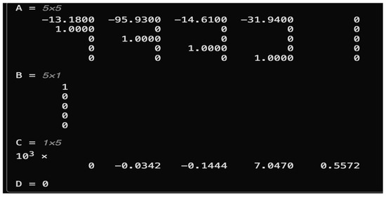
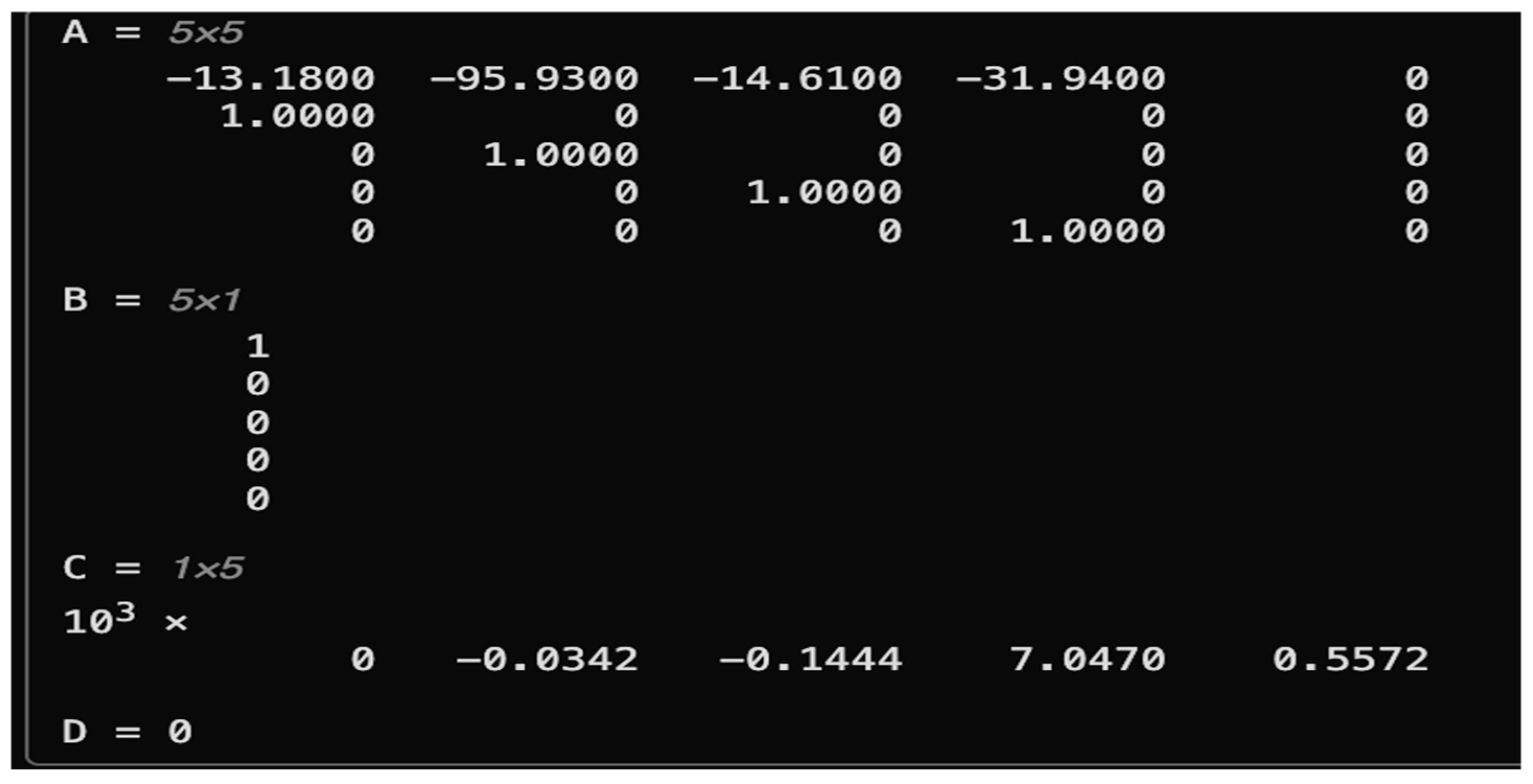
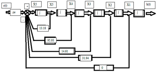
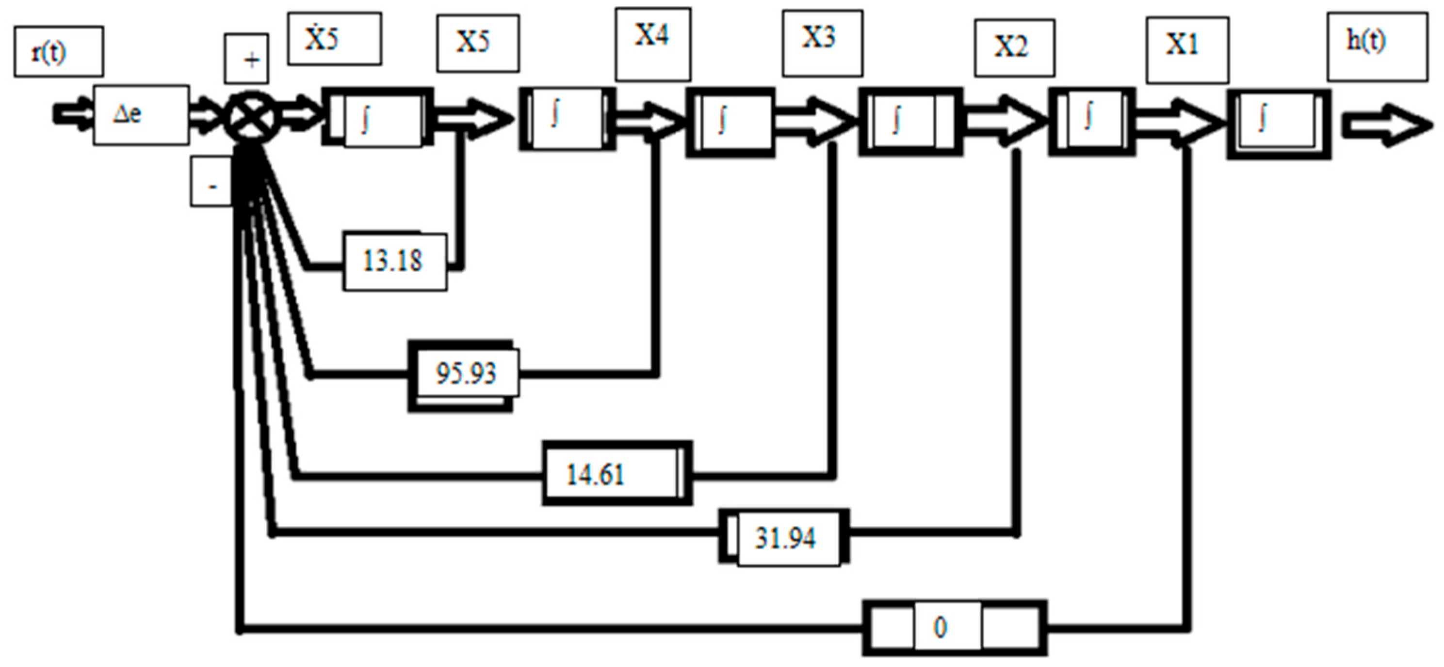
We obtained State-Space representation through MATLAB, mathematically shown in Figure 1 and block diagram representation in Figure 2 by using the Transfer Function.

Figure 1. MATLAB computation of transfer function and state-space matrices.

Figure 2. Block Diagram of the state-space realization.

4.1. Block Diagram from State Space

Denominator Characteristic Equation:

s⁵ + 13.18s⁴ + 95.93s³ + 14.61s² + 31.94s = 0

Let variables:

ẋ₁ = x₂

ẋ₂ = x₃

ẋ₃ = x₄

ẋ₄ = x₅

ẋ₅ = −13.18x₅ − 95.93x₄ − 14.61x₃ − 31.94x₂ − 0·x₁ + B₅·δₑ

State Space Equation:

ẋ₅ = −13.18x₅ − 95.93x₄ − 14.61x₃ − 31.94x₂ + [B₅]δₑ

4.2. Unity Feedback

Transfer Function:

$$v={\displaystyle \frac{-34.16s^3-144.4s^2+7047s+557.2}{s^5+13.18s^4+61.77s^3-129.8s^2+7079s+557.2}}$$

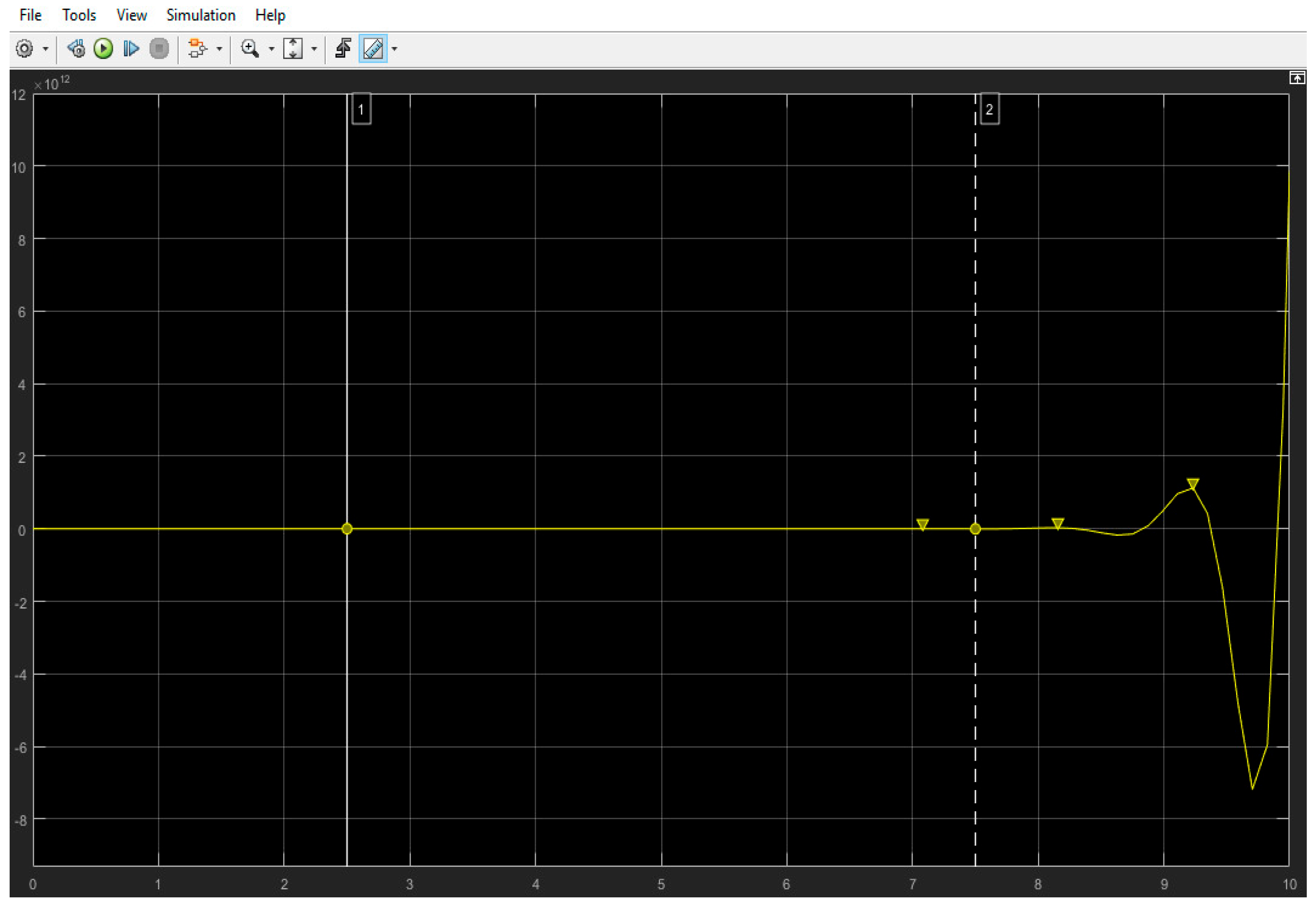
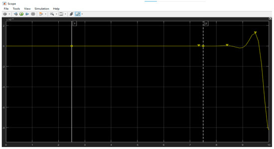
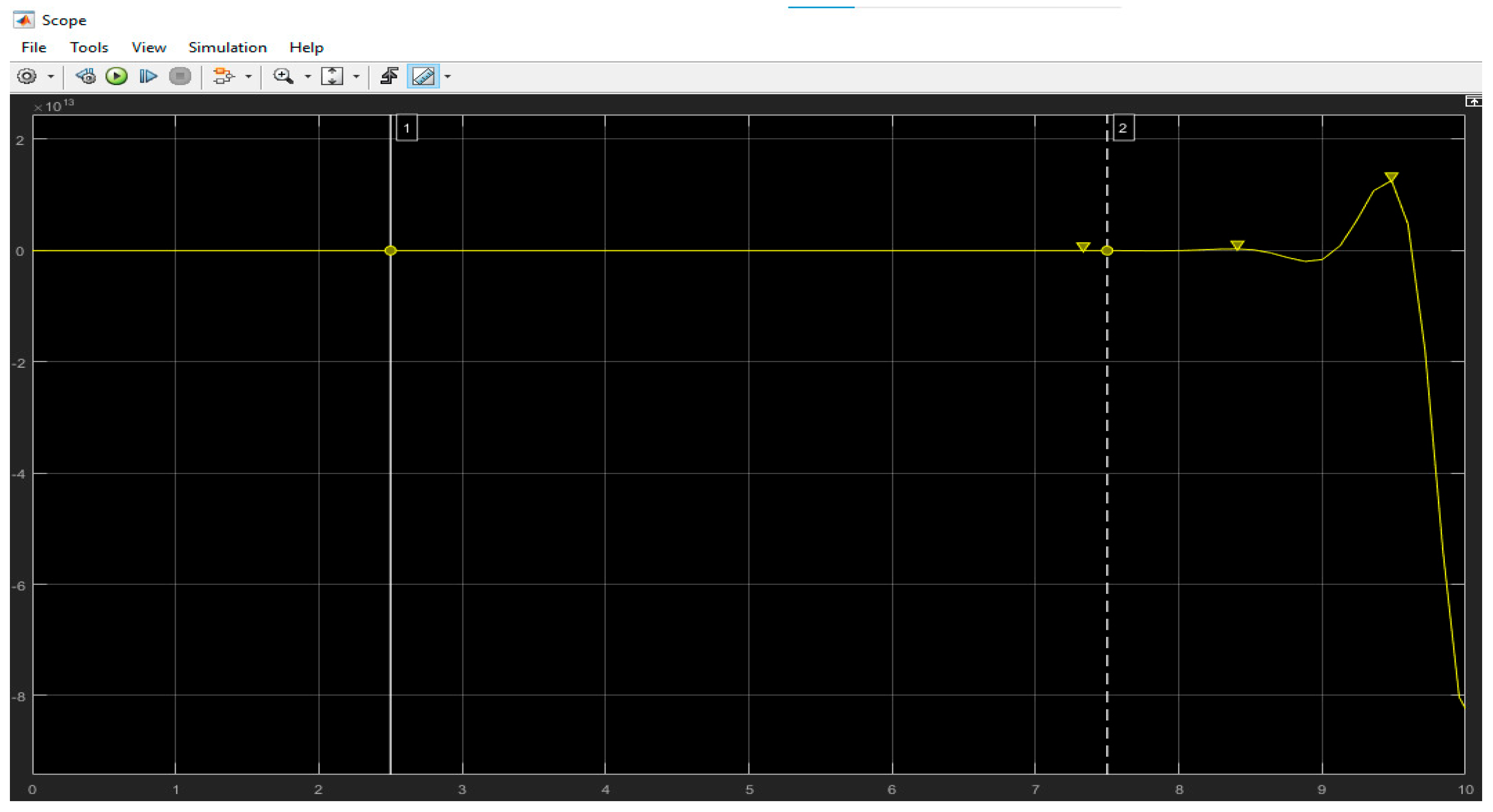
Results Figure 3 demonstrates system response for step input, indicating system instability for the proposed transfer function.

Step Input:

Figure 3. System response for Step-input.

Figure 3. System response for Step-input.

4.3. Characteristics

Results computed and shown in Table 1, indicates damping ratio being negative which shows system has poles on the right half of the plane leading to instability.

Table 1. Time-domain response characteristics of the uncompensated elevator–altitude channel under a step input.

Characteristic	Response
Transient Response	Zero (0)
Steady-State achievement	After many fluctuations
Stability	Not achieved

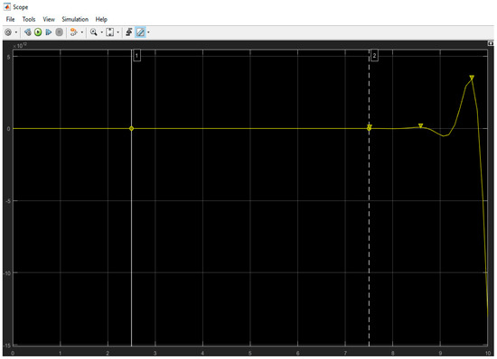
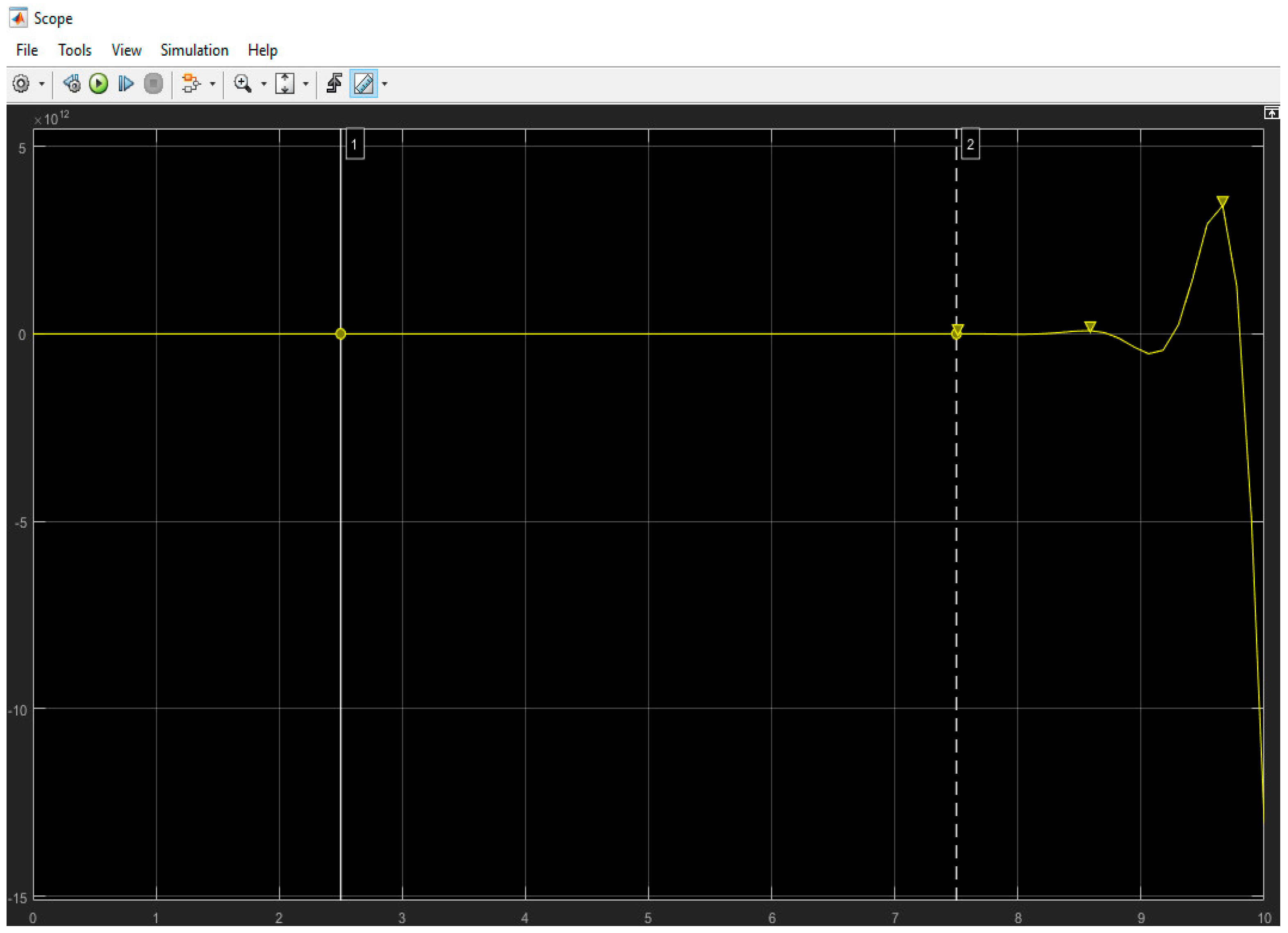
Figure 4 demonstrates response for Ramp Input.

Figure 4. System response for Ramp Input.

Figure 5 demonstrates response for Parabolic Input.

Figure 5. System Response for Parabolic Input.

Table 2 represents characteristics for uncompensated system under parabolic input and Table 3 represents characteristics for reduced second order model.

Table 2. Time-domain response characteristics of the uncompensated elevator–altitude channel under a parabolic input.

Characteristic	Response
Transient Response	Zero (0)
Steady-State achievement	After many fluctuations
Stability	Not achieved

Reduced Second order Transfer Function:

$$\mathit{G}\left(\mathit{s}\right)={\displaystyle \frac{0.3137s^2-6.377s+46.27}{s^2-6.927s+46.27}}$$

G(s) shows continuous-time transfer function for reduced second order.

Table 3. Characteristics of the reduced second-order model.

Characteristic	Values
Settling Time	System Unstable
Overshoot	Unbounded Response
Damping Ratio	Positive Real Poles

Table 3. Characteristics of the reduced second-order model.

Characteristic	Values
Settling Time	System Unstable
Overshoot	Unbounded Response
Damping Ratio	Positive Real Poles

4.4. Root Locus

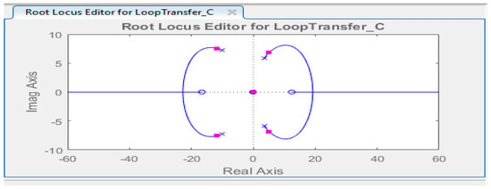
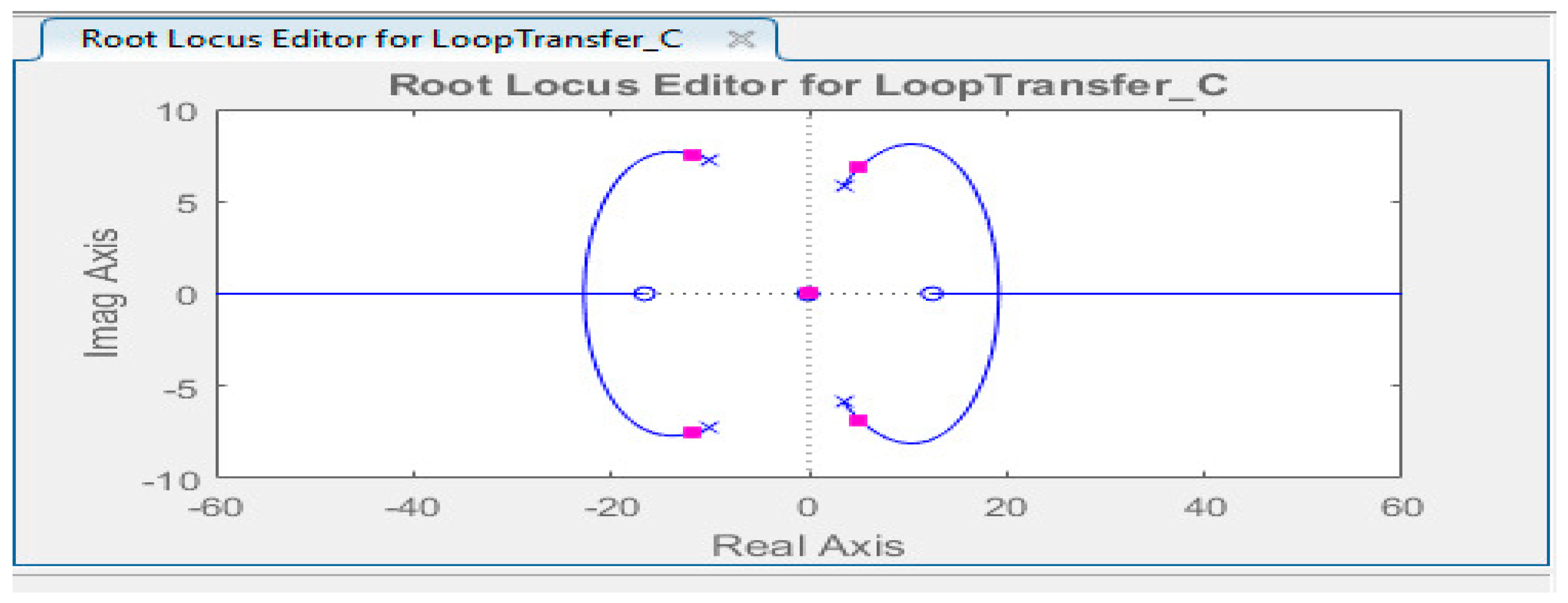
Root Locus is another way to judge the stability of the system. Figure 6 clearly shows that the Root Locus for the transfer function yields a system which is unstable.

Figure 6. Root locus of the uncompensated elevator–altitude channel, showing pole migration into the right-half plane and confirming instability under unity feedback.

The elevator–altitude channel plant is:

$$P\left(s\right)={\displaystyle \frac{-34.16{\mathrm{s}}^3-144.4{\mathrm{s}}^2+7047\mathrm{s}+557.2}{{\mathrm{s}}^5+13.18{\mathrm{s}}^4+95.93{\mathrm{s}}^3+14.61{\mathrm{s}}^2+31.94\mathrm{s}}}$$

Designing PID for Disturbance Rejection

The closed loop Transfer Function is:

$$C\left(s\right)=Kp+{\displaystyle \frac{Ki}{s}}+Kd·s={\displaystyle \frac{Kd·s^2+Kp·s+Ki}{s}}$$

With numerical values:

$$K_p=9.3393\times {10}^{-7}, K_i=9.339262088013577\times {10}^{-7}, \mathrm{and} K_d=0.$$

Practically, the controller acts as a PI law with negligible proportional and integral gains and no derivative term.

With the above plant and controller, the unity-feedback closed-loop transfer function is:

$$\mathrm{T}\left(\mathrm{s}\right)={\displaystyle \frac{\mathrm{C}\left(\mathrm{s}\right)\mathrm{P}\left(\mathrm{s}\right)}{1+\mathrm{C}\left(\mathrm{s}\right)\mathrm{P}\left(\mathrm{s}\right)}}$$

Substituting the above gains into C(s) and forming T(s) in MATLAB yields the closed-loop model used for the time-response plots in Figure 4, Figure 5 and Figure 6 and the performance metrics.

Using MATLAB, this becomes numerically

$$T\left(s\right)={\displaystyle \frac{6\left(s+5\right)}{\left(s+1\right)\left(s+2\right)\left(s+3\right)\left(s+4\right)}}$$

Having poles at −1, −2, −3 and −4

$$G\left(s\right)={\displaystyle \frac{6\left(s+5\right)}{\left(s+1\right)\left(s+2\right)\left(s+3\right)\left(s+4\right)}}$$

The transfer function consists of single zero and four poles that are modelled in MATLAB with output delay of 1 unit and gain of 6 units.

$$\text{The 4th-order model} G\left(s\right)={\displaystyle \frac{6\left(s+5\right)}{\left(s+1\right)\left(s+2\right)\left(s+3\right)\left(s+4\right)}}$$

This is used only as an illustrative benchmark for desired pole locations; the actual closed-loop dynamics with the implemented gains $\left(K_p,K_i,K_d\right)$ are obtained numerically via MATLAB from $T\left(s\right)=C\left(s\right)P\left(s\right)/\left(1+C\left(s\right)P\left(s\right)\right)$.

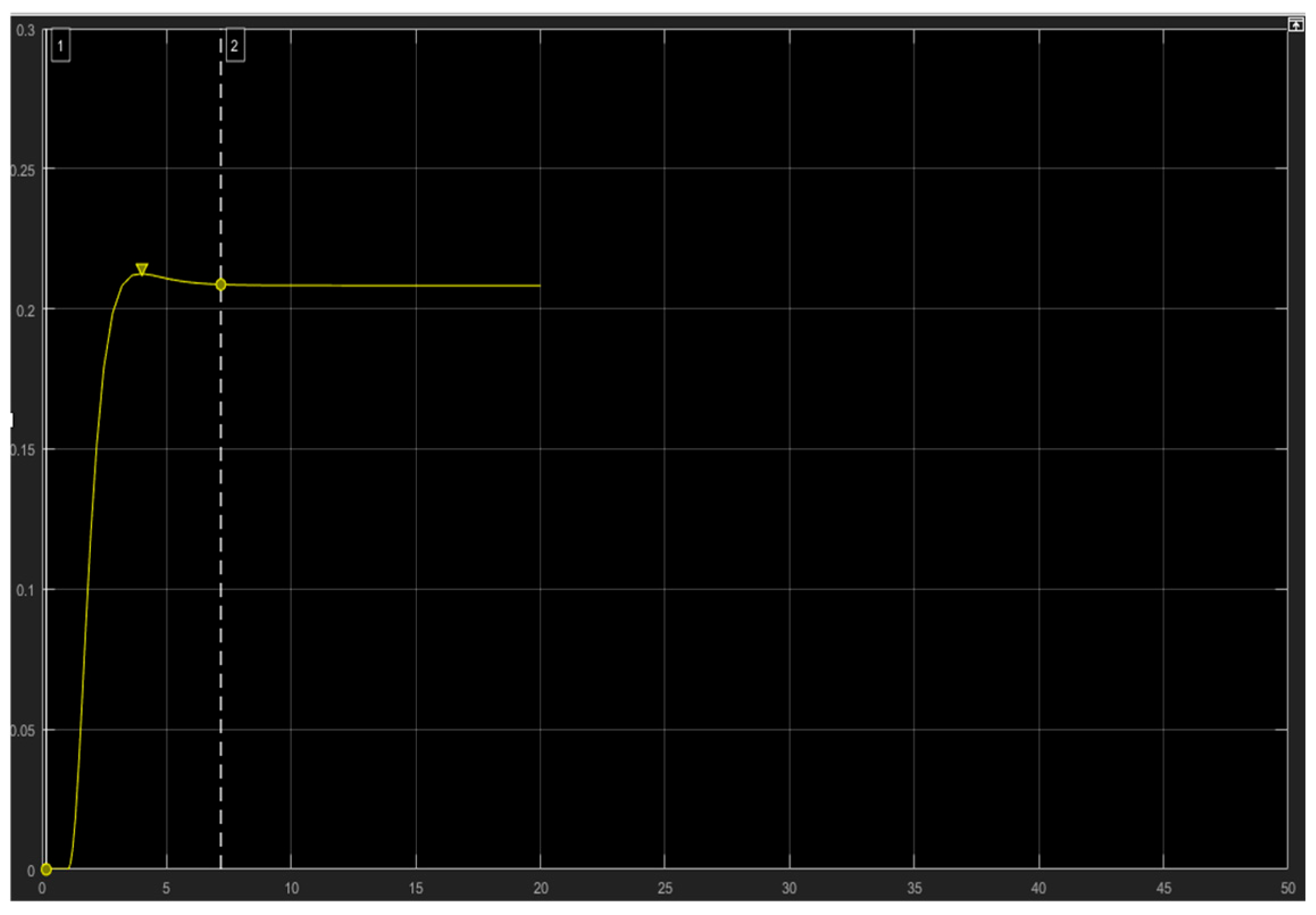
When step input is applied to system having PID controller it reaches the stability with very less steady state error which is suitable for our problem i.e., system is stable with step input as shown in Figure 4. The step input function response shown in Figure 7 computed on the transfer function using MATLAB demonstrates that the system reaches stability.

Step Input given to G(s):

Figure 7. Step response of the PI-controlled elevator–altitude channel, showing a stable response with low steady-state error.

Figure 7. Step response of the PI-controlled elevator–altitude channel, showing a stable response with low steady-state error.

Ramp Input:

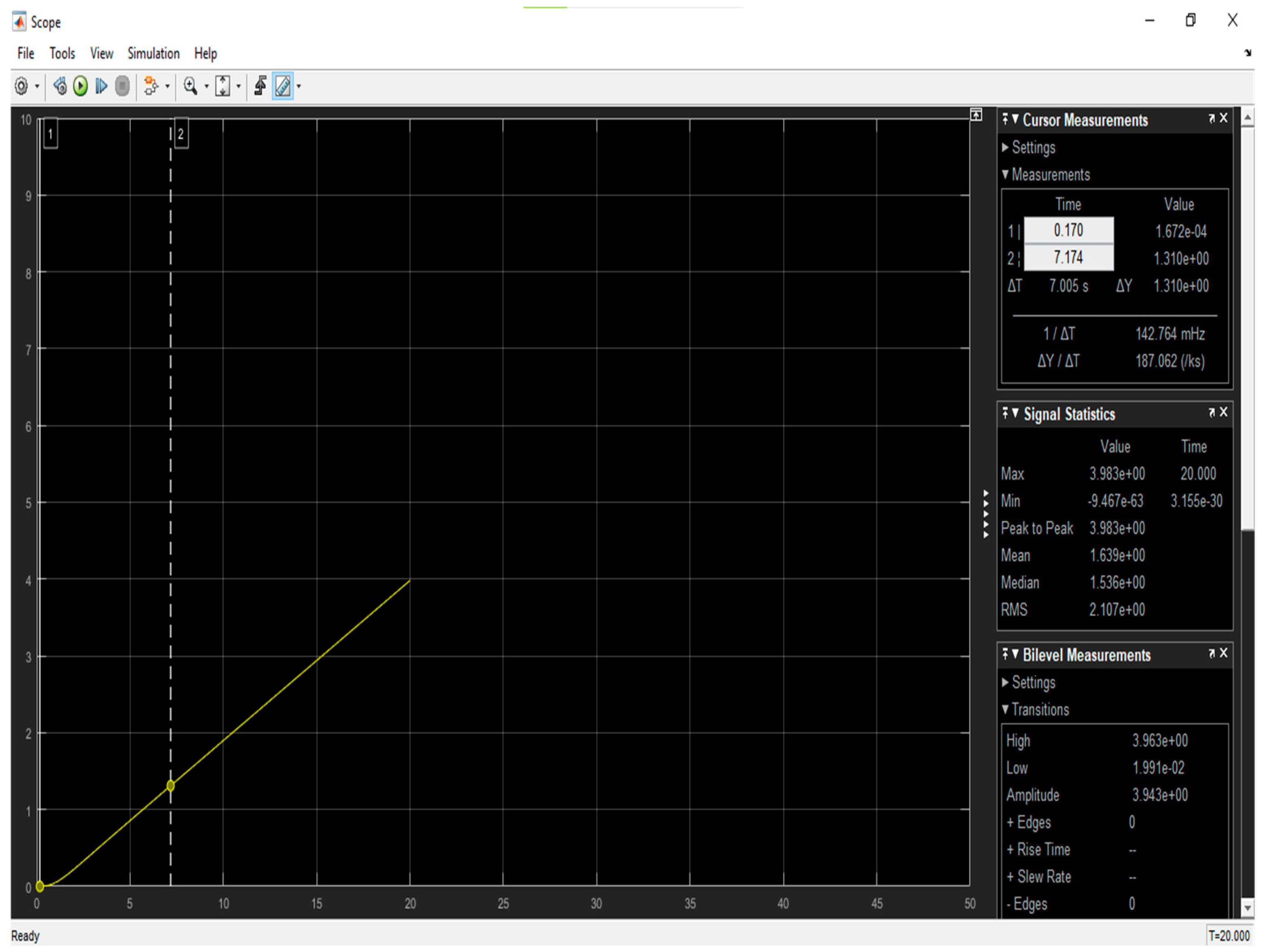
When a ramp input is applied to the system, output constantly increases as the input is increased. Because the ramp input is such that the input is constantly increasing i.e., the system approaches instability and steady state error becomes infinite. Below Table 2 shows the results for the ramp input shown in Figure 8, indicate a settling time of 7.174 for the system to reach stability.

Response:

Figure 8. Ramp response of the PI-controlled system, showing bounded transient behavior but nonzero steady-state tracking error, consistent with a type-0 system.

Figure 8. Ramp response of the PI-controlled system, showing bounded transient behavior but nonzero steady-state tracking error, consistent with a type-0 system.

When parabolic input is given to system it approaches instability and steady state error becomes infinite as shown in Figure 9 and characteristics identified in Table 4.

Parabolic Input:

Figure 9. Parabolic response of the PI-controlled system, showing divergence in tracking error for a higher-order input, consistent with the steady-state error analysis.

Figure 9. Parabolic response of the PI-controlled system, showing divergence in tracking error for a higher-order input, consistent with the steady-state error analysis.

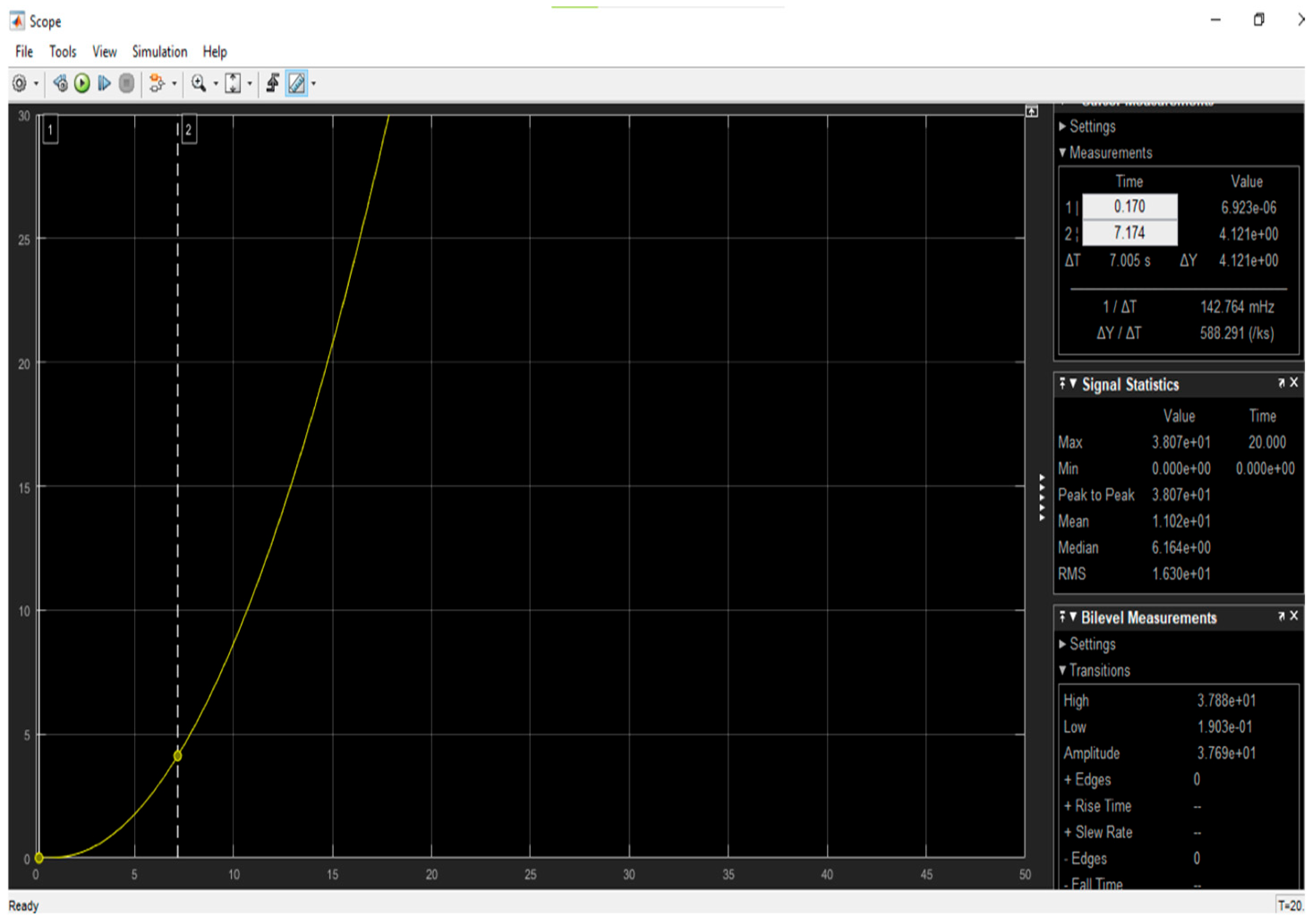
Table 4. Time-domain performance indices of the PI-controlled elevator–altitude channel under a ramp input.

Characteristic	Response
Settling Time	7.174
Peak Time	4 s
Percentage Overshoot	1.5%
Rise time	1.288 s

Table 4. Time-domain performance indices of the PI-controlled elevator–altitude channel under a ramp input.

Characteristic	Response
Settling Time	7.174
Peak Time	4 s
Percentage Overshoot	1.5%
Rise time	1.288 s

5. Stability

For finding the stability, we are using closed loop transfer function. From Routh table, Table 5, the s¹ row element is 50 − 8K. For stability, all elements in the first column of the Routh table must be positive. This yields the inequalities 50 − 8K > 0, i.e., K < 6.25, and 24K > 0, i.e., K > 0. Therefore, the admissible stability range is 0 < K < 6.25.

Table 5. Routh array for the closed-loop characteristic polynomial.

$\mathrm{G}\left(\mathrm{s}\right)={\displaystyle \frac{6\left(\mathrm{s}+30\right)\mathrm{K}}{{\mathrm{s}}^4+10{\mathrm{s}}^3+35{\mathrm{s}}^2+50\mathrm{s}+24\mathrm{K}}}$

$\left(\begin{array}{ccc}1& 35& 24\hspace{0.17em}K\\ 10& 50& 0\\ 30& 24\hspace{0.17em}K& 0\\ 50-8\hspace{0.17em}K& 0& 0\\ 24\hspace{0.17em}K& 0& 0\end{array}\right)$

In the simulations we select K = 3, which lies well inside this range and provides a compromise between fast response and robustness to parameter variations.

Steady State Error:

In order to find the steady state error, the step input is applied to the system. We consider a unity-feedback configuration where G(s) denotes the open-loop transfer function after compensation, and the closed-loop transfer function is $T\left(s\right)=G\left(s\right)/1+G\left(s\right)$ [8]. The error calculated as:

$${lim}_{s\to 0}\mathrm{G}\left(\mathrm{s}\right)={\displaystyle \frac{180 K}{24K}}={\displaystyle \frac{180}{24}}=7.5$$

The factor K cancels and the DC gain is independent of the choice of $K$ within the stability range.

For a unit step input in unity feedback, the steady-state error is:

$$\mathrm{e}\left(\mathrm{\infty }\right)={\displaystyle \frac{1}{1+{lim}_{s\to 0}\mathrm{G}\left(\mathrm{s}\right)}}={\displaystyle \frac{1}{1+7.5}}=0.118$$

For the ramp input the steady state error will be:

$$\mathrm{e}\left(\mathrm{\infty }\right)={\displaystyle \frac{1}{{lim}_{s\to 0}\mathrm{G}\left(\mathrm{s}\right)\mathrm{s}}}=\mathrm{\infty }$$

For the parabolic input the steady state error will be:

$$\mathrm{e}\left(\mathrm{\infty }\right)={\displaystyle \frac{1}{{lim}_{s\to 0}{s}^2\mathrm{G}\left(\mathrm{s}\right)}}=\mathrm{\infty }$$

Root Locus

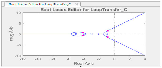
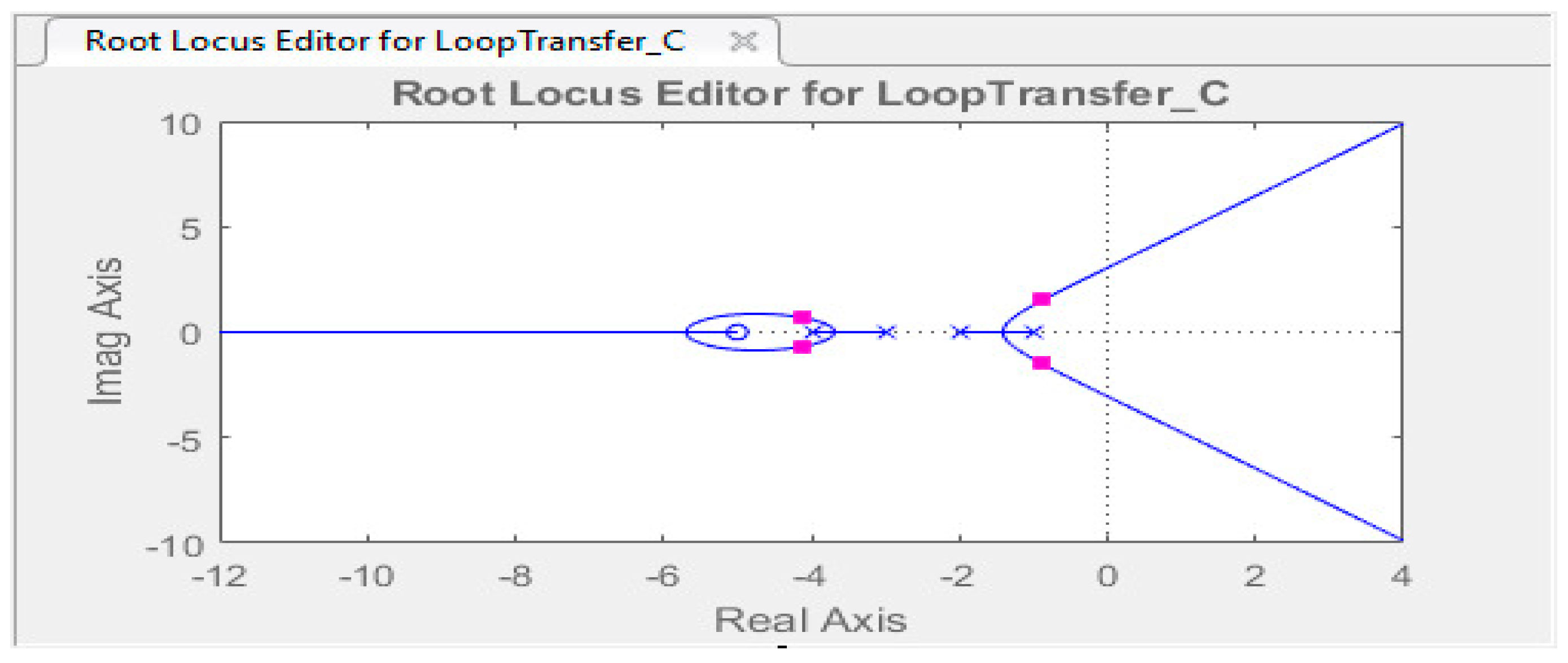
Figure 10 shows a stable Root Locus for the PID-Controller, indicating the system is stable. The system has reached stability after the introduction of PID-Controller.

Figure 10. Root locus of the PI-compensated system for the selected gain, showing that the dominant poles remain in the left-half plane.

6. Conclusions

Almost all existing autopilots use PID-based controllers for altitude regulation. In this paper, altitude control through elevator deflection was studied using a linearized fixed-wing UAV model. The uncompensated elevator–altitude channel was shown to be unstable under unity feedback, while the compensated system achieved improved transient response and a finite steady-state error for step commands. The present results should be interpreted as a baseline linear design for altitude hold around a trim condition. Extending this framework to explicitly nonlinear or time-varying controllers for larger operating envelopes is an important direction for future work. Overall, the study demonstrates that a PI-based elevator controller can stabilize the altitude channel of a UAV modeled via a linearized transfer function and can provide a practical benchmark for future work in advanced UAV control design.

References

- Harden, M.C.; Shin, J.Y. Controlling Elevator to Stabilizer Offload in Fly-By-Wire Aircraft Systems. U.S. Patent No. 20180037313, 8 February 2018. [Google Scholar]
- Nise, N.S. Control Engineering Nice, 7th ed.; Wiley: New York, NY, USA, 2015. [Google Scholar]
- Cui, Y.; Liang, Y.; Luo, Q.; Shu, Z.; Huang, T. Resilient Consensus Control of Heterogeneous Multi-UAV Systems with Leader of Unknown Input Against Byzantine Attacks. IEEE Trans. Autom. Sci. Eng. 2025, 22, 5388–5399. [Google Scholar] [CrossRef] [Scilit]
- Cui, Y.; Cheng, L.; Basin, M.; Wu, Z. Distributed Byzantine-Resilient Learning of Multi-UAV Systems via Filter-Based Centerpoint Aggregation Rules. IEEE/CAA J. Autom. Sin. 2025, 12, 1056–1058. [Google Scholar] [CrossRef] [Scilit]
- Imran, I.H.; Alyazidi, N.M.; Eltayeb, A.; Ahmed, G. Robust Adaptive Fault-Tolerant Control of Quadrotor Unmanned Aerial Vehicles. Mathematics 2024, 12, 1767. [Google Scholar] [CrossRef] [Scilit]
- Khanzada, H.R.; Maqsood, A.; Basit, A. Artificial Intelligence in UAV Flight Controls: Deep Reinforcement Learning Based Altitude-Hold Strategies for Fixed-Wing UAVs. IEEE Access 2025, 13, 109670–109686. [Google Scholar] [CrossRef] [Scilit]
- Yang, F.; Yuan, R.; Yi, J.; Fan, G.; Tan, X. Direct adaptive type-2 fuzzy neural network control for a generic hypersonic flight vehicle. Soft Comput. 2013, 17, 2053–2064. [Google Scholar] [CrossRef] [Scilit]
- Li, C.; Yi, J.; Wang, M.; Zhang, G. Monotonic type-2 fuzzy neural network and its application to thermal comfort prediction. Neural Comput. Appl. 2012, 23, 1987–1998. [Google Scholar] [CrossRef] [Scilit]
- Ngoc, H.T.B.; Binh, B.V. Investigation of aerodynamics and longitudinal stability of unmanned aerial vehicle with elevator deflection. Vietnam. J. Mech. 2019, 41, 89–103. [Google Scholar] [CrossRef] [Scilit] [PubMed]
- Ma, H.; Gao, Y.; Yang, Y.; Xu, S. Improved Nonlinear Model Predictive Control Based Fast Trajectory Tracking for a Quadrotor Unmanned Aerial Vehicle. Drones 2024, 8, 387. [Google Scholar] [CrossRef] [Scilit]
- He, H.; Huo, M.; Duan, H.; Deng, Y.; Wei, C. Distributed Cooperative Control of Human–UAV Swarm Based on State Observation. IEEE Trans. Syst. Man. Cybern. Syst. 2025, 55, 7335–7345. [Google Scholar] [CrossRef] [Scilit]
Disclaimer/Publisher’s Note: The statements, opinions and data contained in all publications are solely those of the individual author(s) and contributor(s) and not of MDPI and/or the editor(s). MDPI and/or the editor(s) disclaim responsibility for any injury to people or property resulting from any ideas, methods, instructions or products referred to in the content. |
© 2026 by the authors. Licensee MDPI, Basel, Switzerland. This article is an open access article distributed under the terms and conditions of the Creative Commons Attribution (CC BY) license.