Reinforcement Learning for Plasma Control: A Proof of Concept for NTM Suppression

Abstract

Neoclassical tearing modes (NTMs) are magnetohydrodynamic instabilities that generate magnetic islands in tokamak plasmas, degrading confinement and potentially limiting high-performance operation. Their stabilization typically requires precise alignment and appropriate injection of electron cyclotron (EC) power beams, making real-time control a challenging task. In this work, we present a proof-of-principle study aimed at investigating the potential role of neural networks in the control of plasma instabilities. The objective is not the design of a controller for a specific machine, but rather to study how a learning-based agent can autonomously discover effective stabilization strategies through reinforcement learning. A synthetic environment based on a tokamak scenario is used as a test bed for this investigation; the specific scenario plays no essential role in the methodological conclusions. The controller is trained using reinforcement learning techniques and operates solely on a representation of the magnetic island width, without relying on equilibrium reconstruction or explicit knowledge of the deposition location relative to the island. Two control tasks are considered: pure angular alignment and combined angular alignment with power control. The strategies that autonomously emerge are consistent with hand-designed approaches reported in the literature, while the framework remains flexible for incorporating additional objectives such as power minimization. This exploratory study establishes a framework for assessing the potential advantages of data-driven approaches in magnetic island control and provides a basis for future investigations aimed at improving alignment and suppression strategies in fusion plasmas.

1. Introduction

In a tokamak, the plasma equilibrium is described on nested toroidal magnetic surfaces. Each surface is characterized by a safety factor q, defined as the local ratio of the toroidal and poloidal angular increments along a magnetic field line. Surfaces on which q takes a rational value $m/n$ are called rational surfaces: on these, the field lines close on themselves after m toroidal turns and n poloidal turns. These surfaces are particularly susceptible to magnetohydrodynamic (MHD) instabilities. Neoclassical tearing modes (NTMs) are MHD instabilities that arise on these rational surfaces in tokamak plasmas [1,2,3,4]. When destabilized, NTMs lead to the formation of magnetic islands that perturb the magnetic topology and degrade energy confinement. If left uncontrolled, their growth can significantly reduce plasma performance and, in severe cases, trigger a complete loss of equilibrium (disruption). The relevance of NTMs for tokamak operation is well documented. A survey of unintentional disruptions at the Joint European Torus (JET) performed by de Vries et al. [5] reported that approximately 16% of the analyzed disruptions were associated with the presence of NTMs, making them the single most frequent identified cause among the considered cases. Real-time detection and control of NTMs are, therefore, of fundamental importance for ensuring stable plasma operation. This is particularly critical in high-performance regimes, characterized by elevated plasma pressure (high $\beta$), where the operational margins are reduced, and the impact of magnetic islands is more severe. The issue becomes even more pressing for next-generation devices such as ITER, where the machine is designed to tolerate only a limited number of disruptions over its operational lifetime [6]. The amplitude of an NTM can be controlled by driving a localized current at the O-point of the magnetic island. This externally driven current compensates for the deficit in bootstrap current, which constitutes the primary drive of the island during its nonlinear evolution phase [7]. By restoring the current profile locally, the destabilizing mechanism can be mitigated and the island growth arrested. In practice, this control strategy is implemented through the injection of electron cyclotron (EC) power beams, which enable localized current drive and heating. In future machines, NTM suppression will have more demanding requirements on ECH/CD alignment. Nowadays, real-time control systems for NTM suppression typically rely on a sequence of coordinated operations: the detection of the magnetic island, the identification of its radial position through equilibrium reconstruction, and the subsequent alignment of the EC launcher so that the injected power is deposited at the island O-point [8,9]. Achieving accurate alignment requires establishing the relationship between the beam deposition location and the poloidal injection angle $\alpha$. The overall control architecture, therefore, depends on the consistent interaction of diagnostic measurements, equilibrium reconstruction, wave propagation modeling, and actuator control. In this work, we propose to investigate a neural-network-based controller trained through reinforcement learning for the stabilization of magnetic islands. The application of reinforcement learning to NTM control has been performed before [10], but focusing on global $\beta$ control to prevent the triggering conditions for an NTM.

Different active NTM control strategies not using equilibrium reconstruction have been addressed using the response of the islands to the EC as the main control command. The ‘Search and suppress’ scheme, as in [11], uses an MHD sensitivity marker to stop a predefined angular scan of the ECRH launcher close to the rational surface. Alignment can be refined using optimum seeking methods, as the one implemented in [12]. Merging the two algorithms would require the implementation of logic (state machine) switching between the two functionalities. Nevertheless, these kinds of algorithms are limited to just steering the ECH launcher, not to optimizing the amount of the injected power, which will be essential in future machines like DTT and ITER, where several launchers and power sources are installed. In [13], a physics-driven estimation of the power requested is proposed by running in real-time the equations governing the island evolution. However, this calculation, again, requires information from equilibrium and ray/beam tracing codes. In this work, we investigate whether reinforcement learning can provide a tool in which these aspects are integrated within a single policy. Firstly, we develop an RL to properly align the ECH/CD injection at fixed power; then, we study the possibility of introducing ECH/CD power optimization in the RL control task. The objective is not to provide a device-specific control solution, but rather to conduct a proof-of-concept study within a synthetic environment, with the aim of assessing both the potential and the limitations of this approach. For this reason, we exploited the Proximal Policy Optimization (PPO) [14] algorithm, a policy-based, model-free reinforcement learning method that directly optimizes a stochastic policy through interaction with the environment. By avoiding the construction of an explicit model of the system dynamics, PPO reduces the dependence on a specific analytical representation of the plasma. The controller is trained to act on two control variables: the injected power and the poloidal injection angle. As feedback, the agent receives an estimate of the magnetic island amplitude. This can be obtained using a diagnostic signal proportional to the amplitude of the instability. The magnetic measurements and cyclotron emission have been proven to be suitable within this scope [15,16,17]. In this framework, the behavior of the controller is not dictated by an explicit control model. Rather, it is shaped through the reward function provided by the environment. By modifying the reward structure, different control objectives and constraints can be enforced, allowing the learning process to autonomously converge toward optimized stabilization strategies. In Section 2, the reinforcement learning framework is introduced. A description of the problem and the training process is given in Section 3 and Section 4. In Section 5, the agent is optimized in order to minimize the power used to stabilize the magnetic island.

2. Reinforcement Learning Framework

The system under consideration, namely, the magnetic island evolving under the plasma conditions, is a dynamic system whose behavior can be influenced through external actuators. The role of the controller is to manipulate the suppression system in order to drive the island toward a desired state, typically complete stabilization. Such a setting can be formally described within the framework of a Markov Decision Process (MDP). An MDP provides a mathematical representation of sequential decision-making in a dynamic environment, where a decision maker (agent) interacts with the system over time [18]. In this formalism, at each discrete time step t, the decision-maker observes the current state $s_t$ of the system and selects an action $a_t$. The action influences the subsequent evolution of the dynamic system, leading to a new state $s_{t+1}$. At each time step t, the agent selects an action $a_t$ according to a policy $\pi \left(a_t\right|s_t)=P(a_t\mid s_t)$, a function that specifies the probability of executing a certain action, given that the system is in state $s_t$ at time t. The objective of the decision-maker is to select actions so as to optimize system performance $G_{\gamma }\left(t\right)$ over future states. $\gamma \in (0,1]$ is a free parameter, named the discount factor, that quantifies how the effect of an action taken at time t propagates into future states by weighting the contribution of subsequent rewards. For $\gamma =0$, system performance is determined solely by the instantaneous reward. Conversely, when $\gamma =1$, all rewards throughout the process are weighted equally. The policy ${\pi }^{*}\left(a\right|s)$ that, at each time step t, selects actions so as to maximize the expected return $G_{\gamma }\left(t\right)$ is referred to as the optimal policy. In the present context, the magnetic island dynamics and the status of the actuators (power source and launching angle) represent the environment, while the controller acts as the decision-maker. The control problem is, therefore, recast as a sequential decision process in which the policy determines how the actuator should be operated, based on the current state. Within this framework, the agent is implemented as a neural network that, by virtue of its well-known universal approximation capability [19], is able to approximate the optimal policy ${\pi }^{*}\left(a\right|s)$ through a dedicated training procedure known as reinforcement learning [20,21]. This section introduces the reinforcement learning framework underlying the present work and describes the components of the learning system. Section 2.1 formalizes the control problem as a Markov decision process and outlines the general reinforcement learning loop. Section 2.2 describes the environment, including the physical model used to evolve the magnetic island (Section 2.2.1) and the reward function designed to drive the agent toward suppression (Section 2.2.2). Section 2.3 introduces the Proximal Policy Optimization algorithm adopted for training, together with the structure of the loss function (Section 2.3.1). Finally, Section 2.4 details the neural network architecture.

2.1. Reinforcement Learning

In reinforcement learning, the policy ${\pi }_{\theta }\left(a_t\right|s_t)$ is represented by a neural network, where $\theta$ denotes the set of trainable parameters of the model. The network maps the current state of the system to a probability distribution over the available actions ${\pi }_{\theta }\left(a_t\right|s_t)=P_{\theta }(a_t\mid s_t)$. During training, the parameters $\theta$ are iteratively updated so as to optimize (minimize) a loss function $L\left({\pi }_{\theta }\left(a_t\right|s_t)\right)$. The update is performed by moving in the direction opposite to the gradient ${\nabla }_{\theta }L\left({\pi }_{\theta }\left(a_t\right|s_t)\right)$, according to standard gradient-based optimization procedures. The loss function is constructed such that its minimization corresponds to the maximization of the expected return $G_{\gamma }\left(t\right)$. The training process consists of a sequence of parameter updates, here referred to as iterations. At the i-th iteration, the policy is denoted as ${\pi }_{\theta }^{\left(i\right)}\left(a_t\right|s_t)$, reflecting the current set of parameters ${\theta }^{\left(i\right)}$. As training progresses, successive updates modify the policy in order to increase the expected return. Under suitable conditions and for a sufficiently large number of iterations, the sequence of policies may converge toward an optimal policy: ${\pi }_{\theta }^{\left(i\right)}\left(a_t\right|s_t)\to {\pi }^{*}\left(a_t\right|s_t)\mathrm{as}i\to \infty .$ In this way, adjusting the network parameters through gradient descent leads the policy to progressively improve its long-term performance. This approach belongs to the class of policy-based methods, in which the policy itself is directly parameterized and optimized. In order to enlarge as much as possible the portion of the state–action space explored by the agent, each training iteration i includes a rollout phase during which multiple episodes are executed using the current policy ${\pi }_{\theta }^{\left(i\right)}$. An episode corresponds to one complete rollout of the agent–environment interaction, from initialization to termination. During each episode, trajectories are collected in the form of sequences of state–action transitions. More precisely, for $t=1,\dots ,T_{\mathrm{episode}}$, a trajectory is a set of $\left\{s_t,a_t,{\pi }_{\theta }^{\left(i\right)}\left(a_t\right|s_t),G_{\gamma }\left(t\right)\right\}$, where $T_{\mathrm{episode}}$ denotes the episode length. These trajectories of an iteration constitute the dataset used to estimate the loss function $L\left({\pi }_{\theta }^{\left(i\right)}\right)$ and compute the gradient update of the policy parameters. The trajectories collected during the rollout phase are generated through the interaction between the agent and the environment. At each time step t within an episode, the agent selects an action $a_t$, sampled following the current policy, the environment evolves to a new state, and a reward $r_t$ is returned according to a predefined reward function. The reward $r_t$ provides an instantaneous evaluation of system performance at time t, based on criteria established in the formulation of the control objective. In this sense, the reward function encodes the performance metrics that define what constitutes desirable behavior for the controlled system. For each trajectory, the return $G_{\gamma }\left(t\right)$ is then computed as an aggregation of the reward $r_t$ at each time step. In particular, it is defined as the discounted sum of future rewards:

$$G_{\gamma }\left(t\right)={\displaystyle \sum _{k=0}^{T_{\mathrm{episode}}-t}}{\gamma }^k{r}_{t+k}.$$

(1)

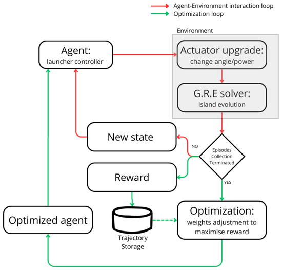
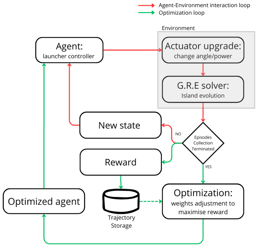
As summarized in Figure 1, reinforcement learning provides a framework for training an agent to follow an optimal control strategy for a given task by iteratively adjusting its policy based on the rewards returned by the environment at each time step.

Figure 1. Illustration of the interaction loop between agent and environment (red) and the optimization loop that trains the agent (green).

In the present work, the environment is represented by the numerical model that evolves the magnetic island dynamics, explicitly accounting for the influence of the injected power on its temporal evolution.

The agent is implemented as a neural network composed of a Long Short-Term Memory (LSTM) layer, followed by fully connected layers.

The reward function is designed to promote island suppression: the agent receives positive reinforcement when the island width decreases and negative feedback otherwise. In addition, the reward includes penalty terms enforcing physical constraints, in particular, limiting the admissible angular excursion of the launcher. The policy parameters are optimized using the Proximal Policy Optimization (PPO) algorithm.

2.2. Environment

The environment consists of a synthetic model that simulates the temporal evolution of the magnetic island. The dynamics are discretized in time steps of 10 ms. At each time step, the agent selects an action, corresponding to a modification of the injected power or the poloidal angle. This action is applied to the simulation environment, and its effect is incorporated into the island evolution over the subsequent 10 ms interval. The updated state of the island (width and growth rate) is then returned to the agent, closing the interaction loop. A simulation (episode) terminates either when a maximum of 300 time steps is reached or when the island width decreases below a predefined threshold of 1 mm, which is taken as a condition for complete suppression. The evolution is based on the DTT [22] full power scenario [23], in which there will be 8 MW of power coming from the upper launcher dedicated to the control and suppression of NTMs. The EC power deposition from the upper launcher used for NTM suppression is computed using the GRAY ray-tracing code [24]. A preliminary scan over the poloidal injection angle is performed to compute the EC power deposition profile corresponding to each angle. The resulting deposition profiles are subsequently retrieved during the simulation through a lookup table. The considered angles span the interval between 7° and 26°. Within this range (assumed to represent the admissible angular excursion of the launcher), the network is allowed to adjust the injection angle, changing it by a quantity $\delta \alpha$ at each step. The island evolution is computed under the assumption of a fixed-plasma equilibrium. In particular, the feedback of the magnetic island on global plasma transport is neglected, so that the background equilibrium profiles are kept constant throughout the simulation. This assumption enables the construction of a computationally lightweight simulation environment, which can be iterated over a large number of times during training. In the following section, the physical model for the evolution of the NTM will be explained.

2.2.1. NTM Evolution Model

The temporal evolution of the magnetic island width is modeled through a generalized Rutherford equation [25], which relates the growth rate of the island to the combined effect of destabilizing and stabilizing contributions acting on the local current density. In this framework, the island dynamic is governed by a first-order nonlinear ordinary differential equation of the form [26,27]:

$${\displaystyle \frac{dW}{dt}}={\displaystyle \frac{r_s^2}{{\tau }_r{g}_1}}\left({\Delta }_0^{\prime }\left(W\right)+{\Delta }_{bs}^{\prime }\left(W\right)-{\Delta }_{GGJ}^{\prime }\left(W\right)-{\Delta }_{stab}^{\prime }(W,P_{ec},\alpha )\right),$$

(2)

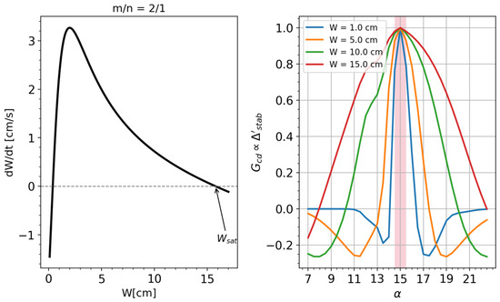
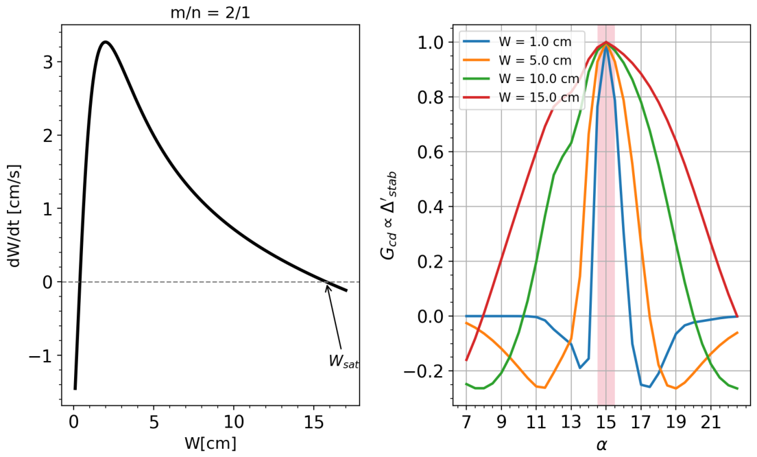
where W denotes the island width, $r_s$ the radial position of the resonant surface, ${\tau }_r$ the resistive time and $g_1=0.82$ [26,28]. The various ${\Delta }^{\prime }$ terms represent the physical mechanisms contributing to the island evolution. The term ${\Delta }_0^{\prime }\left(W\right)$ accounts for the classical tearing stability index [1] and decreases with increasing island width [29]. The bootstrap-driven contribution ${\Delta }_{bs}^{\prime }\left(W\right)$ [2] represents the destabilizing effect associated with the reduction in bootstrap current inside the island due to profile flattening. Stabilizing contributions include the Green–Glasser–Johnson [30] curvature term ${\Delta }_{GGJ}^{\prime }\left(W\right)$ and the active control term ${\Delta }_{stab}^{\prime }(W,P_{ec},\alpha )$. Both the definition of ${\Delta }_{bs}^{\prime }$ and ${\Delta }_{GGJ}^{\prime }$ follow the definition provided by Lazzaro et al. [26]. It is noteworthy that, while ${\Delta }_{GGJ}^{\prime }$ depends on stabilizing phenomena naturally occurring in a tokamak, the ${\Delta }_{stab}^{\prime }$ term depends on the poloidal injection angle $\alpha$ and the injected power. Indeed, this term models the stabilizing effect of the heating ${\Delta }_h^{\prime }$ and that of the current drive ${\Delta }_{cd}^{\prime }$. The definitions of the terms ${\Delta }_{cd}^{\prime }$ and ${\Delta }_h^{\prime }$ are taken from De Lazzari et al. [31]. Figure 2 provides an overview of the model and the physical problem underlying Neoclassical Tearing Mode (NTM) evolution. The left panel illustrates the free evolution curve in the phase space composed of $(\dot{W},W)$ for the $2/1$ mode. It is worth noting that the physical model implies that the evolution of the mode is inherently a nonlinear problem. The right panel depicts the $G_{CD}$ term. This parameter is proportional to ${\Delta }_{stab}^{\prime }$ and accounts for the misalignment between the power deposition location $r_{dep}$ and the position of the rational surface $r_s$. In the control problem is a function of the poloidal injection angle $\alpha$.The curve has a bell shape, peaked at the optimal alignment ${\alpha }_{opt}\simeq 15°$, and this narrows as W decreases. Given the chosen control resolution $\delta \alpha =1°$, the maximum residual misalignment compatible with this discretization is half a degree, corresponding to the angular interval $[14.5°,15.5°]$ highlighted by the red shaded band. In the worst case ($W=1$ cm $<W_{cd}$), the stabilizing term retains approximately $93\%$ of its peak value within this band, which we consider acceptable. This argument supports the choice of $\delta \alpha =1°$ as a sufficient control resolution. The relationship between $r_{dep}$ and $\alpha$, along with other $\alpha$-dependent quantities (deposition width, current drive/heating efficiency and equilibrium quantities related to the effect of the EC), was previously computed using GRAY code and incorporated into the simulation via a lookup table. All the quantities entering the generalized Rutherford equation are computed from equilibrium parameters characterizing the reference plasma scenario. In the present study, these parameters are extracted from a single time snapshot of a DTT integrated simulation performed in [23] with the JETTO–JINTRAC suite [32]; the general features of the scenario are summarized in Table 1.

Figure 2. (Left) Free evolution of the magnetic island width W, obtained from Equation (2) in the absence of external stabilization, for the 2/1 mode. (Right) Stabilizing contribution $G_{cd}\propto {\Delta }_{stab}^{\prime }$ as a function of the poloidal injection angle $\alpha$, evaluated at three values of the island width ($W=1$, 10, 15 cm) for the $2/1$ mode. The red shaded band corresponds to the angular interval of width $\delta \alpha =1°$ centered on the optimal alignment, representing the largest residual misalignment compatible with the chosen control resolution.

Table 1. Reference plasma parameters and NTM characteristics used in this work. The top section reports the global equilibrium parameters of the DTT full-power scenario [23]; the bottom section reports the parameters specific to the 2/1 mode.

Equilibrium Parameters
Toroidal field $B_T$ [T]	5.85
Plasma current $I_p$ [MA]	5.5
Poloidal beta ${\beta }_p$	0.33
Heating scheme	EC (32.0) + ICRH (8.0) + NBI (10.0)
EC power available for NTM control [MW]	8
Confinement time [s]	0.134
NTM Parameters
	2/1 mode
Resonant surface position $r_s$ [m]	0.562
Saturated island width $W_{sat}$ [cm]	16
Optimal injection angle ${\alpha }_{opt}$ [deg]	15
Minimum suppression power [MW]	2.81
Resistive time [s]	0.223
Saturation time [s]	7.5

The equilibrium profiles provide the necessary information on quantities such as the safety factor, pressure gradients, and geometric factors, which determine the various ${\Delta }^{\prime }$ contributions governing the island evolution. In this configuration, the 2/1 island saturates to a $W_{sat}\simeq 16$ cm (as shown in Figure 2(left)), and the power required to fully suppress the saturated island is $2.81$ MW using a continuous injection perfectly aligned with the O-point. This power corresponds to the marginal power computed following Lazzaro et al. [26], at which the island settles at the marginal width. At this point, the suppression time formally becomes infinity: any practical operating point requires a finite margin above this value. Furthermore, angular misalignment between the deposition and the O-point further raises the power requirements. The equilibrium quantities entering these terms are kept fixed, while the stabilizing contribution ${\Delta }_{stab}^{\prime }$ depends on the control actions selected by the agent, namely, the injected power and the poloidal injection angle. The fixed-equilibrium approximation neglects the back-reaction of the island on the global kinetic profiles. The EC deposition profile is weakly sensitive to such perturbations, while the associated degradation of confinement is partially accounted for by reducing $\beta$ as a function of the island width, capturing the dominant feedback on the bootstrap drive. Keeping the equilibrium quantities fixed also enables the rapid and repeated execution of the code, which is necessary for training the agent. At the beginning of each episode, the magnetic island is initialized with a width of 10 cm. This setup represents a control scenario in which no pre-emptive stabilization strategy is applied, and the suppression process begins after the island has already grown to a significant amplitude. At each time step, the selected action modifies the stabilizing term, and the generalized Rutherford equation is integrated over a 10 ms interval to obtain the updated island width.

2.2.2. Reward Function

The scalar reward is computed in the environment as the sum of three active components: (i) a distance-to-target variation term, (ii) a growth-rate magnitude term, and (iii) a launcher-angle threshold penalty. The total reward is defined as

$$r\left(t\right)=r_{\delta W}\left(t\right)+r_{\delta \dot{W}}\left(t\right)+p_{\alpha }\left(t\right).$$

(3)

The first component measures the variation of the absolute distance from the target width:

$$r_{\delta W}\left(t\right)=5\times {10}^2\left(W(t-1)-W\left(t\right)\right).$$

(4)

This term rewards reductions in the distance to $W=0$. It is positive when the island approaches the target and negative when it moves away. Its magnitude depends on how fast the island approaches zero. The second component promotes large island growth-rate magnitude:

$$r_{\delta \dot{W}}\left(t\right)=-10\left(\left|\dot{W}(t-1)\right|-\left|\dot{W}\left(t\right)\right|\right)$$

(5)

This formulation encourages the agent to prioritize dynamically evolving regimes over steady-state saturation. This term represents a shaping potential $\mathsf{\Phi }\left(t\right)=|\dot{W}\left(t\right)|$, a specific functional form that has been theoretically proven to preserve the optimal policy [33]. In practice, this term effectively eliminates the local minima that often lead the neural network to accept island saturation as an acceptable outcome.

An additional penalty term is introduced to discourage persistent attempts to move the launcher beyond its admissible angular limits. Let $n_{\mathrm{viol}}\left(t\right)$ denote the number of consecutive time steps up to time t during which the agent attempts to move the launcher outside the allowed angular range. If such a violation occurs, the following penalty is applied:

$$p_{\alpha }\left(t\right)=-0.2n_{\mathrm{viol}}\left(t\right).$$

(6)

If no violation is detected at time t, the counter is reset:

$$n_{\mathrm{viol}}\left(t\right)=1$$

(7)

This mechanism introduces a progressively increasing cost for repeated boundary violations. Unlike a fixed penalty applied independently at each time step, the linear accumulation in $n_{\mathrm{viol}}$ penalizes persistent boundary-pushing behavior more severely than isolated events. From a control perspective, this term promotes the learning of admissible control strategies within operational constraints. The three coefficients in Equation (3) enforce a hierarchy between the reward components. The coefficient $5\times {10}^2$ of $r_{\delta W}$ is calibrated so that the term produces values of order unity per step (given typical per-step variations of W of ∼${10}^{-2}$ cm), making it the dominant signal driving the optimization. The coefficient 10 of $r_{\delta \dot{W}}$ is intentionally smaller, consistent with its role as a shaping regularizer rather than a primary objective. The coefficient $0.2$ of $p_{\alpha }$ is chosen so that the cumulative penalty remains below the magnitude of the main reward, even after several consecutive boundary violations, preventing the agent from minimizing the penalty at the expense of stabilization. These scales were tuned empirically.

2.3. Training Algorithm

The Proximal Policy Optimization (PPO) algorithm [14] is a policy-based and model-free reinforcement learning method. This formulation naturally supports stochastic policies, which favor exploration of the action space. Moreover, policy-based methods allow the straightforward incorporation of intrinsic motivation mechanisms, such as curiosity-driven exploration [34], enabling the agent to discover novel strategies beyond those induced solely by the external reward. PPO is also a model-free algorithm. In this setting, the agent does not construct or approximate an explicit model of the environment dynamics, i.e., it does not estimate the transition probability distribution $P(s_{t+1}\mid s_t,a_t)$. This characteristic reduces the dependence of the controller on a specific analytical representation of the system dynamics. In complex systems such as plasmas, different operating conditions and physical parameters may lead to a qualitatively different response of the system. Designing a controller based on an explicit model tailored to a particular configuration can, therefore, limit its applicability to other scenarios. A model-free approach mitigates this issue, as the policy is learned directly from interaction data rather than being tied to a predefined transition model of a specific plasma configuration. PPO is typically implemented within an actor–critic architecture [35]. In this framework, the learning system is composed of two complementary components: the actor, which represents the policy, and the critic, which evaluates its performance. In the present implementation, both components are incorporated within a single neural network using a multi-head structure. A shared part of the network processes the input state, after which two distinct output branches are defined. The actor head outputs the stochastic policy ${\pi }_{\theta }\left(a\right|s)$, i.e., the probability distribution over the available actions. The critic head provides an estimate of the expected return, commonly referred to as the value function:

$$V_{\theta }\left(s_t\right)={\mathbb{E}}_{{\pi }_{\theta }}\left[G_{\gamma }\left(t\right)\mid s_t\right],$$

(8)

The critic, therefore, supplies an estimate of the long-term performance associated with a given state. The critic plays a central role in guiding the policy update. Its output $V_{\theta }\left(s_t\right)$ represents the expected return conditioned on the current state, i.e., the performance that the network anticipates when the system is in a given configuration. In other words, for a fixed state $s_t$, the critic estimates how well the agent is expected to perform in the future if it continues to follow the current policy. Based on this estimate, the advantage function is introduced to quantify how beneficial a specific action is compared to this expectation. For a given time step t, the advantage is defined as

$$A_t=G_{\gamma }\left(t\right)-V_{\theta }\left(s_t\right),$$

(9)

where $G_{\gamma }\left(t\right)$ is the realized (discounted) return and $V_{\theta }\left(s_t\right)$ is the critic’s estimate. The advantage, therefore, measures the discrepancy between the actual performance obtained along a trajectory and the performance predicted by the critic. If $A_t>0$, the executed action has led to better-than-expected performance and is, thus, advantageous. Conversely, if $A_t<0$, the action has degraded performance relative to the critic’s expectation. The magnitude of $A_t$ determines how strongly the policy should be reinforced or penalized: the larger the positive difference between $G_{\gamma }\left(t\right)$ and $V_{\theta }\left(s_t\right)$, the more the corresponding action should be encouraged during the policy update. The advantage is directly used to calculate the loss function of the network.

2.3.1. Loss Function

The training objective of the network is defined as a weighted sum of three components:

$$L\left(t\right)=c_1{L}_{\mathrm{critic}}\left(t\right)+c_2{L}_{\mathrm{actor}}\left(t\right)+c_3\left(i\right)L_{\mathrm{entropy}}\left(t\right),$$

(10)

where $c_1$, $c_2$, and $c_3$ are scalar coefficients controlling the relative contribution of each term. As in standard machine learning procedures, training proceeds by minimizing the total loss L through gradient-based optimization. The critic is trained to approximate the expected return associated with a given state. Its loss function, therefore, measures the discrepancy between the predicted value $V_{\theta }\left(s_t\right)$ and the empirical return $G_{\gamma }\left(t\right)$. This is typically expressed as a distance according to a chosen metric. We considered the mean squared error:

$$L_{\mathrm{critic}}\left(t\right)={\left(V_{\theta }\left(s_t\right)-G_{\gamma }\left(t\right)\right)}^2,$$

(11)

Minimizing $L_{\mathrm{critic}}$ encourages the critic to provide an increasingly accurate estimate of the return.

The actor loss is constructed to reinforce actions that yield a positive advantage while preventing excessively large policy updates. In PPO, this is achieved through the clipped surrogate objective:

$$L_{\mathrm{actor}}=-min\left({\displaystyle \frac{{\pi }_{\theta }^{\left(i\right)}(a_t\mid s_t)}{{\pi }_{\theta }^{(i-1)}(a_t\mid s_t)}}{A}_t,\mathrm{clip}\left({\displaystyle \frac{{\pi }_{\theta }^{\left(i\right)}(a_t\mid s_t)}{{\pi }_{\theta }^{(i-1)}(a_t\mid s_t)}},1-ϵ,1+ϵ\right)A_t\right),$$

(12)

The clipping operator constrains the magnitude of policy updates between successive iterations. Specifically, the ratio ${\displaystyle \frac{{\pi }^{\left(i\right)}(a_t\mid s_t)}{{\pi }^{(i-1)}(a_t\mid s_t)}}$ is limited by the clipping operator, defined as the function of the hyperparameter $ϵ=0.2$ [14]. This operation restricts the ratio to lie within the interval $[1-ϵ,1+ϵ]$, thereby preventing excessively large deviations of the updated policy from the previous one.

In this formulation, the sign of the advantage directly determines the direction of the policy update. If $A_t>0$, the surrogate objective encourages an increase in the probability ${\pi }_{\theta }^{\left(i\right)}\left(a_t\right|s_t)$ of the sampled action, reinforcing behaviors that have produced better-than-expected returns. Conversely, if $A_t<0$, the optimization step reduces the probability of that action, discouraging decisions that have led to lower-than-expected performance. In this way, the actor updates are guided by a relative performance signal: actions are not rewarded or penalized in absolute terms, but according to how much they improve or degrade performance with respect to the critic’s expectation. PPO achieves a balance between policy improvement and training stability: the advantage signal drives the direction of the update, while the clipping function ensures that the step size remains conservative.

The final contribution to the loss function is the entropy term, introduced to promote exploration during training [36]. For a discrete action space with $N_{\mathrm{actions}}$ possible actions, the entropy of the policy at time t is defined as

$$L_{\mathrm{entropy}}=-{\displaystyle \frac{1}{N_{\mathrm{actions}}}}{\displaystyle \sum _{i=1}^{N_{\mathrm{actions}}}}{\pi }_{\theta }^{\left(i\right)}(a_i\mid s_t)log{\pi }_{\theta }^{\left(i\right)}(a_i\mid s_t).$$

(13)

The corresponding loss contribution is constructed so as to maximize this entropy. The entropy term prevents the probability distribution over actions from collapsing prematurely toward a nearly deterministic policy. Without this regularization, the agent may converge too early to a suboptimal strategy, thereby reducing exploration and increasing the risk of being trapped in a local optimum. By maintaining sufficient stochasticity in the action-selection process, the entropy term supports a broader exploration of the control space during training. It is important to note that the coefficient determining the magnitude of the $L_{\mathrm{entropy}}$ depends on the iteration number i. The term $c_3$ decreases linearly from a maximum (larger exploration) at the beginning of the training to a minimum (less exploration) reached at 80% of the training process.

2.4. Neural Network Architecture

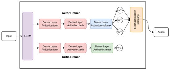
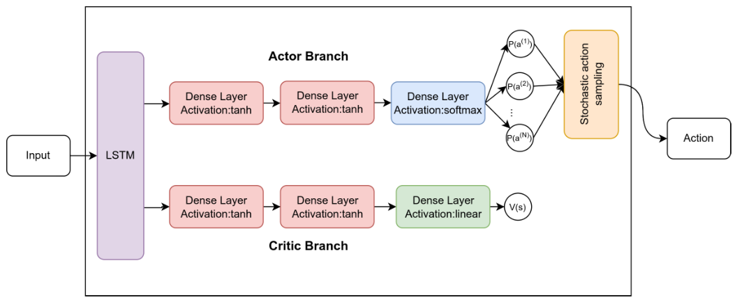
The architecture of the neural network is shown in Figure 3. The input layer of the network is connected to a Long Short-Term Memory (LSTM) module [37,38]. LSTM units are a class of recurrent neural networks specifically designed to handle sequential data. They incorporate internal memory mechanisms that allow the network to conserve and update information over both short and long temporal horizons. Importantly, the parameters governing these memory mechanisms are not predefined: the corresponding weights are learned during training so that the network autonomously determines which features are relevant for the control task. In the present implementation, the LSTM layer is composed of 64 hidden units. The hidden state dimension, therefore, corresponds to 64 features. This configuration enables the network to maintain an expressive internal representation of the temporal evolution of the system. At each time step t within an episode, the LSTM cell receives both the current input observation and its own hidden state $h(t-1)$ from the previous step, producing an updated hidden state $h\left(t\right)$ that encodes the temporal evolution of the system. The hidden state is initialized at the beginning of each episode and is reset at episode termination.

Figure 3. Illustration of the structure of the network. The input is entered in the LSTM module, and then the output of the layer is split into two branches. The Actor branch, composed of a sequence of Dense layers (hyperbolic tangent activation and $\mathrm{softmax}\left(x_i\right)=e^{x_i}/{\sum }_{j=1}^N{e}^{x_j}$ activation), outputs the probability of taking a certain action. The Critic branch, whose structure is the same as the actor branch, outputs the value used to calculate the loss function. The output of the actor branch is used to sample an action to be performed on the environment.

Following the LSTM module, the network splits into two fully connected branches implementing the actor and the critic (multi-head architecture). Both branches take as input the LSTM output and consist of two dense layers with 64 neurons each and a hyperbolic tangent as the activation function. The final layer of the actor branch (actor head) has $N_{\mathrm{actions}}$ output units and a softmax activation layer, whose output integrates to 1, consistent with the meaning of action probability distribution ${\pi }_{\theta }\left(a\right|s)$. The critic branch follows an analogous structure, but its output head consists of a single neuron with linear activation, returning the scalar value estimate $V_{\theta }\left(s\right)$. During both training and evaluation, actions are sampled stochastically from the output of the actor branch, which represents the policy distribution ${\pi }_{\theta }\left(a\right|s)$ [39].

3. Alignment Task with Fixed Power

In this configuration, the agent operates in a discrete action space composed of three possible commands acting on the poloidal launcher angle. At each time step, the agent can either increase the angle by a fixed increment $\delta \alpha$, decrease it by the same amount, or leave it unchanged. The angular step $\delta \alpha$ defines the control resolution and remains constant throughout the training. The state (input) of the system is the island width $W\left(t\right)$, its growth rate $\Delta W/\Delta t=\left(W\left(t\right)-W(t-dt)\right)/dt$, the last executed action $a(t-dt)$, and a binary flag indicating whether the launcher angle was modified at the previous time step (1 if moved, 0 otherwise). The input of the neural network is a 4-dimensional vector. Input quantities and action space is listed in Table 2. The inclusion of the previous action $a(t-dt)$ and the binary flag in the input vector are motivated by two considerations. Since actions are sampled stochastically from the policy, the previous action is not uniquely determined by the previous state, and providing it explicitly improves the consistency of the input representation. The binary flag, in turn, informs the agent whether the previously commanded action was actually executed or inhibited by the angular boundary. The power level injected in the plasma is taken to be fixed and equal to $P=6$ MW. Under these conditions, the learning task was reduced to a pure alignment problem: the agent was required to steer the deposition location toward the resonant surface without being responsible for managing the power. This configuration allows a clear assessment of the agent’s capability to learn optimal angular steering strategies independently of power effects.

Table 2. Action space and state vector (neural network input) used in the angular-only control configuration. The injected power is fixed at $P=6\mathrm{MW}$ and is, therefore, not included as a state variable.

Action Space
Action ID	Command	Description
0	$+\delta \alpha$	Increase launcher angle
1	$-\delta \alpha$	Decrease launcher angle
2	0	Keep launcher angle unchanged
State Vector (Neural Network Input)
Input #	Symbol	Description
1	$W\left(t\right)$	Magnetic island width at time t
2	$\Delta W/\Delta t$	Island growth rate
3	$a(t-dt)$	Last executed action
4	${\mathrm{flag}}_{\alpha }$	1 if launcher angle was updated at previous step, 0 otherwise

3.1. Training

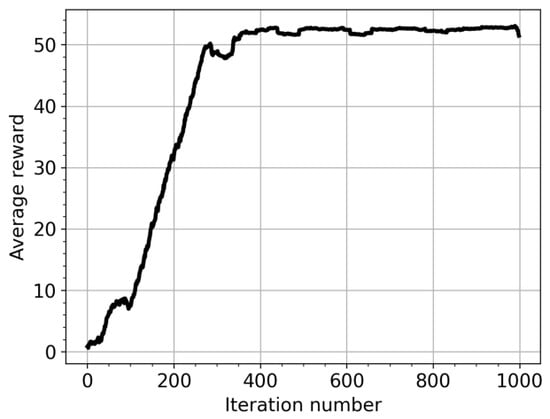
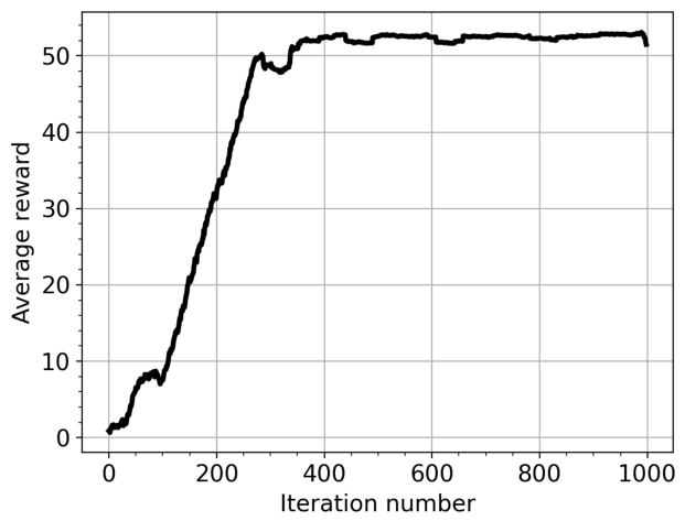
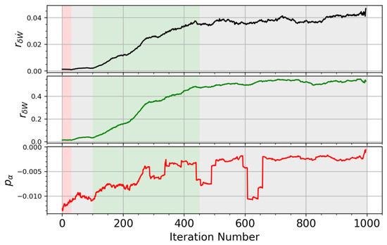
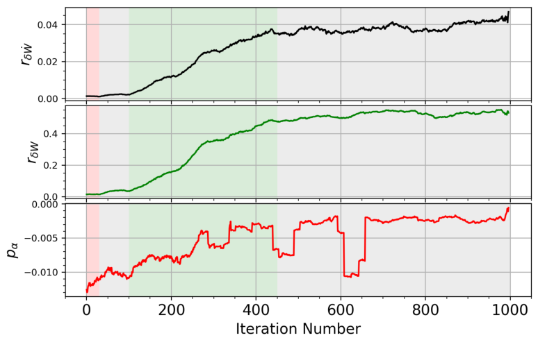
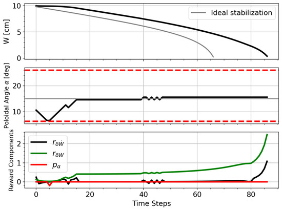
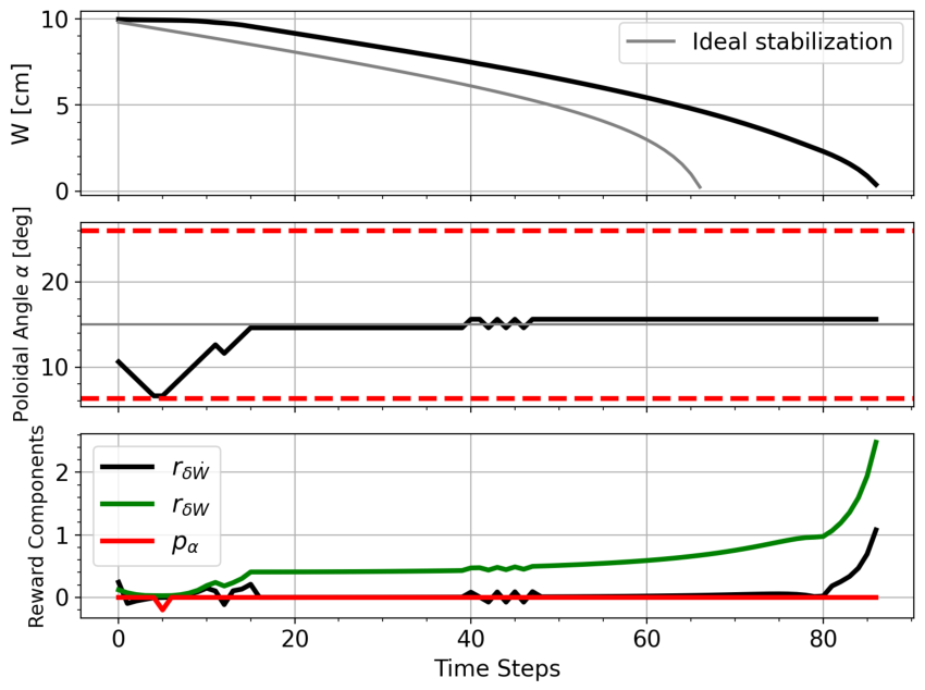
The training dataset is generated during the training itself from the interaction between the agent and the environment, with each iteration producing a new set of trajectories sampled according to the current policy. At the beginning of each training episode, the initial launcher angle is randomly sampled from two intervals, $\alpha \in [7°,12°]$ and $\alpha \in [18°,23°]$. These intervals are deliberately chosen to be far from the optimal alignment so that the agent is never initialized in the vicinity of the optimum during training. The training consists of 1000 iterations, each composed of the rollout of 5 episodes. An episode corresponds to an island evolution until suppression or $t_{max}=3\mathrm{s}$. As a consequence, the agent was never initialized in the vicinity of the optimal angle during training. Training under these constraints was successful and showed stable convergence. Figure 4 shows the progression throughout the training, expressed in terms of the average reward on all the episodes. In particular, a consistent optimal policy emerged after approximately 300–400 training iterations. Above this point, the reward saturates at a value slightly above 50. Figure 5 shows the evolution of the three individual reward components during training. For each iteration, each component is computed by averaging its value over all the time steps collected in the rollout of that iteration. The top plot represents the shaping contribution $r_{\delta \dot{W}}$ aimed at discouraging island saturation, the middle plot corresponds to the main stabilization term $r_{\delta W}$, and the plot at the bottom denotes the angular constraint penalty $p_{\alpha }$. The dominant contribution throughout training is the main stabilization term (green), which drives the overall reward signal. Its evolution closely follows the trend of the total reward, exhibiting a progressive increase as the agent improves its alignment strategy and achieves more effective island suppression. The gradual growth of this component reflects the increasing ability of the policy to produce consistent reductions in island width. Four distinct phases of the learning process can be identified, highlighted by the colored bands in Figure 5. In the first phase (iterations 0–30, red band), only the angular penalty $p_{\alpha }$ shows a clear evolution, progressively decreasing in magnitude, while the two stabilization-related components remain nearly constant and close to zero. In this initial phase, the agent is still moving randomly in the action space, and its first learning achievement is to identify the admissible angular region and avoid persistent boundary violations. The subsequent phase (iterations 30–100, first gray band) corresponds to an exploration regime in which the agent searches the action space without yet producing consistent improvements in any of the reward components. The third phase (iterations 100–450, green band) is the actual policy-learning phase: over approximately 350 iterations, the two stabilization-related terms $r_{\delta W}$ and $r_{\delta \dot{W}}$ grow consistently, while the angular penalty continues to decrease in magnitude. Finally, after iteration ∼450 (second gray band), the reward components saturate, indicating that the policy has converged. Figure 6 shows a representative simulation obtained after the training. At this stage, the training process is close to completion, and the agent is expected to have converged toward the optimal policy. The top panel displays the time evolution of the island width W, the middle panel the poloidal launcher angle at each time step, and the bottom panel the individual components of the reward function. During the first ∼5 time steps, the agent explores the angular space. In this phase, the launcher angle is progressively decreased, moving away from the optimal alignment, until the lower angular boundary is reached. At that point, the agent attempts to further decrease the angle; however, since the physical limit has been reached, the angle no longer changes. When the lower angular boundary is reached, the agent may still select the action corresponding to a further decrease in the launcher angle. However, the actuator saturates at the physical limit, and the commanded action produces no actual angular displacement. This effect is explicitly observable by the agent through the angle flag included in the state vector, which is set to 1 only when the launcher angle is effectively updated and is set to 0 otherwise. Therefore, the agent can learn during the training process that the selected control direction is not feasible because the action does not translate into state evolution, despite being repeatedly chosen. In addition, the reward signal includes the angular penalty term (red curve in the bottom panel), which provides a negative reinforcement for persistent attempts to exceed the admissible angular range and further discourages this behavior. Subsequently, the agent reverses the steering direction and begins increasing the launcher angle. After approximately 10 time steps, the island width starts to decrease, indicating that the deposition is moving toward the resonant surface. From this point onward, the agent consistently reinforces this control direction, steering the launcher toward the optimal alignment and eventually stabilizing around the corresponding angle. The reward components reflect this learning behavior. In the initial phase, strategies leading to island saturation are penalized, as evidenced by the negative contribution of the $r_{\delta \dot{W}}$ term (black line, third plot). Once proper alignment is achieved, the main reward component becomes positive and progressively increases. A sharp growth in the total reward is observed when the island suppression accelerates, highlighting the dominance of the stabilization term as the island approaches complete suppression.

Figure 4. Average reward per iteration over the training process of the network in the angular-only control configuration.

Figure 5. Per-step contribution of the three reward components averaged over each training iteration. From (top) to (bottom): the saturation-avoidance shaping term $r_{\delta \dot{W}}$ (black), the main stabilization term $r_{\delta W}$ (green), and the angular constraint penalty $p_{\alpha }$ (red). The shaded regions highlight different training phases: penalty reduction (red), reward improvement (green), and stationary phases (gray).

Figure 6. Typical behavior of the controller in the alignment task for the stabilization of the 2/1 mode. (Top) Evolution of the island width; The horizontal red lines represents the angular limits of the controller (Middle) value of the injection poloidal angle $\alpha$; (Bottom) components of the rewards.

3.2. Test and Discussion

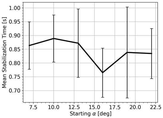
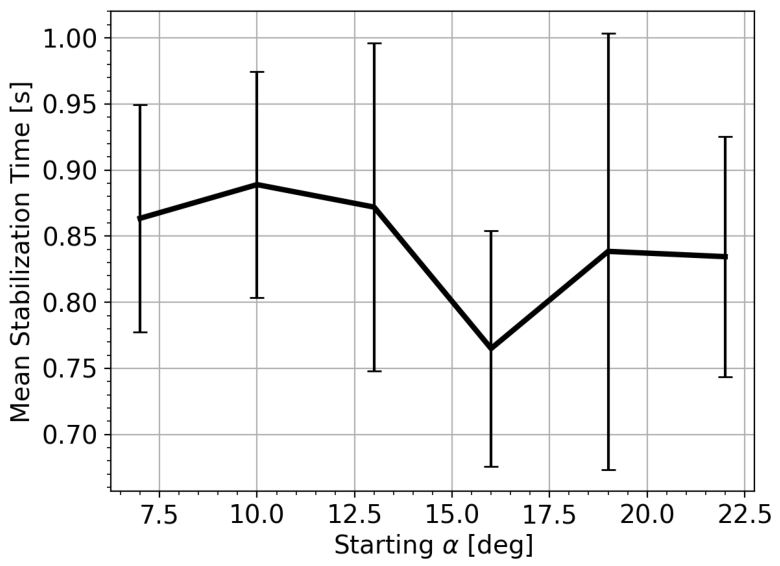
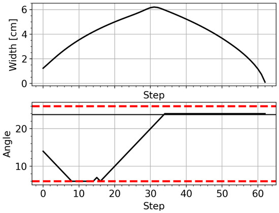
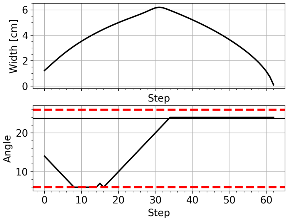
The gray trace in Figure 6 (Top) represents the trajectory of the island in the case of ideal stabilization, i.e., $\alpha =15$ aligned with the O-point of the island, for the same power level. In this case, the island is stabilized in around $0.65$ s. For testing, the suppression time is evaluated on a regular grid of initial launcher angles spanning the entire operational range $\alpha \in [7°,23°]$. This grid includes the central interval $\alpha \in [12°,18°]$ that was never sampled as an initial state during training, allowing the assessment of the agent’s ability to generalize beyond the angular distribution observed in the training phase. For each initial condition, the stabilization time is computed as the average over a statistical ensemble of 20 independent episodes (Figure 7). A clear minimum is observed in the vicinity of $\alpha \simeq 15°$, which corresponds to the optimal alignment with the island O-point. When the initial angle is close to this value, the agent requires minimal corrective action, and stabilization is achieved in the shortest time. Moving away from the optimal angle in either direction results in a progressive increase in the stabilization time. A larger initial angular misalignment implies that the launcher must explore a wider radial region before reaching the optimal deposition location. Consequently, the agent requires additional control steps to identify and reach the stabilization configuration. It is noteworthy that the presence of a well-defined minimum around $\alpha \simeq 15°$ indicates that the learned policy extends coherently across the angular domain, rather than being confined to the regions explored during training. It is important to emphasize that the agent was not provided with any prior information regarding the optimal alignment position. As an assessment of the generalization capability of the trained policy beyond the configuration it was trained on, the same agent was applied without retraining to the suppression of a different magnetic island, namely, a 3/2 mode characterized by a different saturated width, a different radial position of the resonant surface, and an optimal alignment angle of ${\alpha }_{opt}\simeq 23.75°$. An angular scan was performed on a regular grid of initial angles spanning the operational range, with 20 independent rollouts per initial angle. The agent successfully suppressed the 3/2 island in 100% of the rollouts across all tested initial angles (Figure 8 shows an example), despite the optimal alignment being substantially different from that of the 2/1 scenario used for training.

Figure 7. Average stabilization time as a function of the initial launcher angle $\alpha$ for the angular-only control configuration. Each point is computed as the average over a statistical ensemble of 20 independent rollouts of the trained network. Error bars represent the standard deviation across the ensemble.

Figure 8. Representative stabilization trajectory of a 3/2 magnetic island obtained by applying the policy trained on the 2/1 mode without retraining. Top: Time evolution of the island width W. Bottom: Time evolution of the poloidal injection angle $\alpha$; the black horizontal line indicates the optimal alignment angle for the 3/2 mode (${\alpha }_{opt}\simeq 23.75°$); the red dashed lines denote the angular boundaries.

This first test demonstrates that the reinforcement learning framework is capable of autonomously identifying the optimal geometric alignment strategy when the control space is reduced to angular steering alone. The emergence of a stable optimal policy indicates that the reward formulation provides a sufficiently informative and well-shaped learning signal. The agent is able to identify and reinforce the correct alignment strategy without requiring additional heuristic adjustments. Consequently, for the subsequent extensions of the control problem, no structural modification of the reward function is introduced.

4. Alignment Task with Power Control

In this extended configuration, the agent is allowed to control both the launcher angle and the injected EC power. The action space is, therefore, expanded to five discrete actions, acting either on the angular alignment or on the power level. At each time step, the policy may: increase the launcher angle by a fixed increment $\delta \alpha =1°$, decrease it by the same amount, increase the injected power by $1\mathrm{MW}$, decrease it by $1\mathrm{MW}$, or leave both quantities unchanged. The present model does not account for the physical constraints of the gyrotron actuators, such as power ramp rate limits, response delays, and finer power discretization. The chosen $\delta P=1\mathrm{MW}$ per 10 ms step is, therefore, a methodological simplification. A more realistic representation of the actuator dynamics, including these constraints, will be required to assess the deployability of the proposed approach on real systems. The injected power is initialized to zero at the beginning of each episode. Consequently, the agent must not only identify the correct geometric alignment, but also determine when and how rapidly to increase the power in order to suppress the island. The enlargement of the action space increases the complexity of the control task. The state (input) of the system is defined by the island width $W\left(t\right)$, its growth rate $\Delta W/\Delta t=\left(W\left(t\right)-W(t-dt)\right)/dt$, the last executed action $a(t-dt)$, the previously injected power $P(t-dt)$, and a binary flag indicating whether the launcher angle was modified at the previous time step (1 if moved, 0 otherwise). The actions and inputs are summarized in Table 3. Importantly, the reward formulation remains unchanged so that any difference in learning behavior can be attributed to the higher-dimensional control space rather than to modifications of the optimization objective.

Table 3. Action space and state vector (neural network input) used in the alignment task with power control. Compared to the angular-only configuration, the action space is extended to five commands, and the previously injected power $P(t-dt)$ is added as an additional state variable.

Action Space
Action ID	Command	Description
0	$+\delta \alpha =1°$	Increase launcher angle
1	$-\delta \alpha =-1°$	Decrease launcher angle
2	$+\delta P=1\mathrm{MW}$	Increase injected power
3	$-\delta P=-1\mathrm{MW}$	Decrease injected power
4	/	No changes in power and angle
State Vector (Neural Network Input)
Input #	Symbol	Description
1	$W\left(t\right)$	Magnetic island width at time t
2	$\Delta W/\Delta t$	Island growth rate
3	$a(t-dt)$	Last executed action
4	$P(t-dt)$	Previously injected power
5	${\mathrm{flag}}_{\alpha }$	1 if launcher angle was updated at previous step, 0 otherwise

4.1. Training

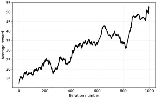
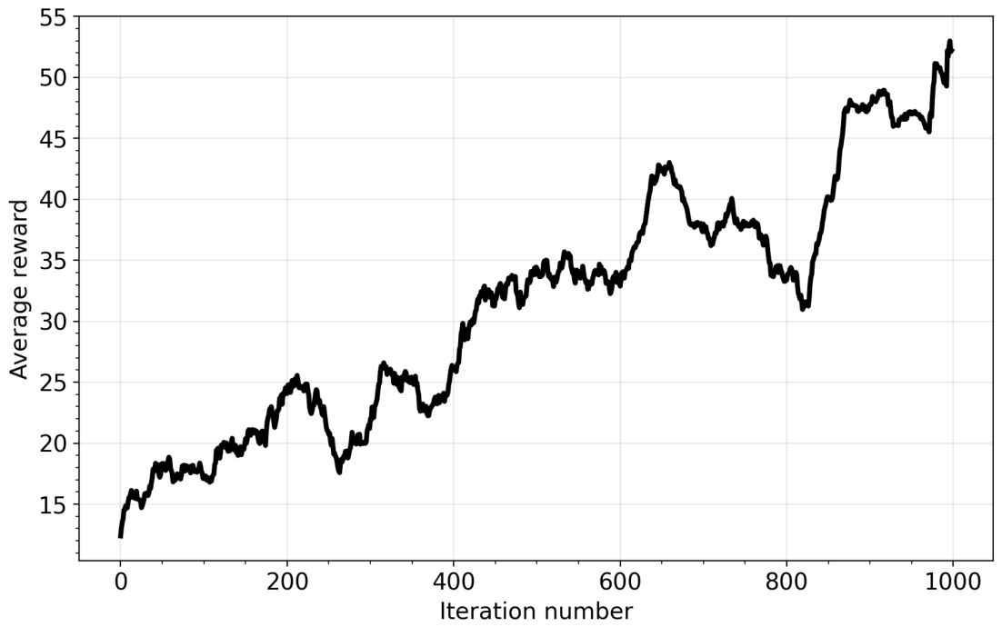
Figure 9 shows the evolution of the average reward during training in the joint angular and power control configuration. The reward function is identical to the one used in the alignment-only task, and training is run for the same number of iterations; the reward magnitudes obtained in the two configurations can, therefore, be compared on the same scale. Relative to the fixed-power case, learning is slower and less stable. The enlarged action space adds complexity to the exploration phase, and the reward consequently exhibits stronger fluctuations and a more gradual improvement over iterations. Even in the late iterations, the reward does not reach the stability observed in the fixed-power case, indicating that convergence is less robust under the current hyperparameter configuration. A marked drop appears around iteration 800, followed by a steep recovery over the final iterations, at the end of which the reward attains values comparable to those of the angular-only configuration. The final performance is not yet optimal, but the controller improves over iterations and provides a viable basis for further refinement.

Figure 9. Average reward per iteration through a complete training process for the alignment task with power control.

4.2. Test and Discussion

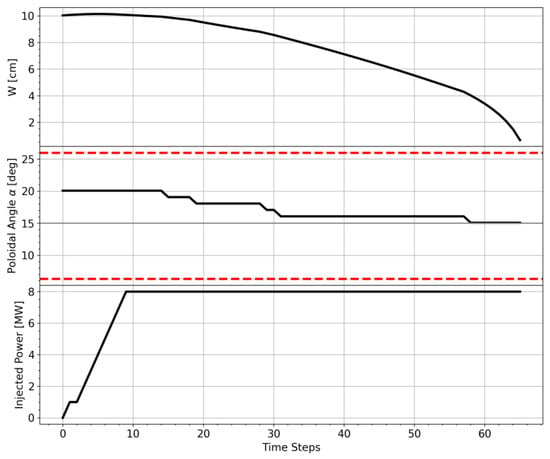
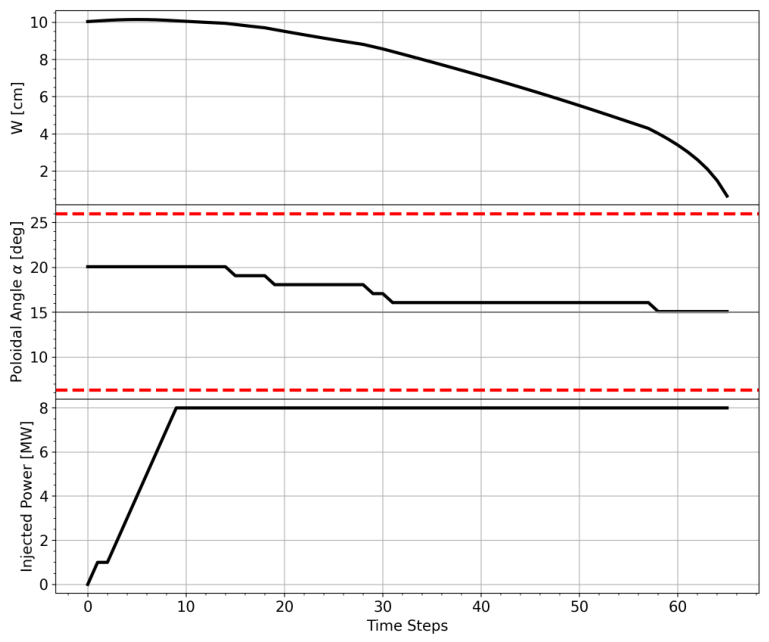
Figure 10 illustrates a representative example of the controller operating under the joint angular and power control configuration at the end of training. During the first ∼10 time steps, the agent increases the injected power in discrete steps of $1\mathrm{MW}$, progressively ramping it up to the maximum available level of 8 MW. In this initial phase, the launcher angle remains essentially unchanged, indicating that the policy prioritizes establishing a sufficient stabilization drive before refining the alignment. Once the power has reached its maximum value, the agent begins adjusting the launcher angle. A reduction in the angle by one increment $\delta \alpha$ produces a measurable decrease in the island width, indicating that the steering direction is correct. The policy then consistently continues to move the launcher in the same direction, applying successive 1° corrections until optimal alignment is reached. After convergence to the optimal angular region, the angle remains approximately constant while the island width decreases monotonically toward suppression. A notable feature of this behavior is that the agent maintains the injected power at its maximum level throughout the stabilization phase. While this strategy is effective in achieving suppression, it is not necessarily optimal from an energetic standpoint. The early and sustained ramp-up of power suggests that the current policy prioritizes rapid stabilization over power efficiency. The optimal policy can be improved, for instance, by delaying the power ramp-up until near-optimal alignment is achieved, thereby reducing unnecessary power usage while preserving stabilization performance.

Figure 10. Typical behavior of the controller in the alignment task for the 2/1 mode. (Top) Evolution of the island width; (Middle) value of the injection poloidal angle $\alpha$. The horizontal red lines represents the angular limits of the controller; (Bottom) value of the injected power.

5. Power Optimization

In order to promote a more energy-efficient control strategy, the reward function was further modified by introducing an additional cost term penalizing the use of high injected power. Starting from the previously trained network controlling both poloidal angle and injected power, a new training phase was performed with the modified reward function. The additional power cost is formulated as a hinge-like function, i.e., a piecewise-linear term that remains zero below a prescribed threshold and increases beyond it,

$$C_p=-\lambda max{\left(0,P-P_{\mathrm{th}}\right)}^2,$$

(14)

where P is the injected power, $P_{\mathrm{th}}$ is a predefined threshold, and $\lambda$ controls the strength of the penalty. The threshold $P_{th}$ is set at $40\%$ of the maximum available power ($3.2$ MW out of 8 MW), slightly above the marginal suppression power (∼2.8 MW, Section 2.2). This small margin allows the agent to reach the power level actually required for suppression, while penalizing only the excess beyond this operationally relevant value. The maximum power available for the stabilization is 8 MW, and the threshold power above which the network is penalized is set to be at 40% of the maximum power. The quadratic dependence ensures moderate power exceedances are only mildly discouraged, whereas significantly high power levels are strongly penalized. This modification is intended to discourage unnecessarily large power levels while still allowing the agent to exploit them when strictly required for stabilization.

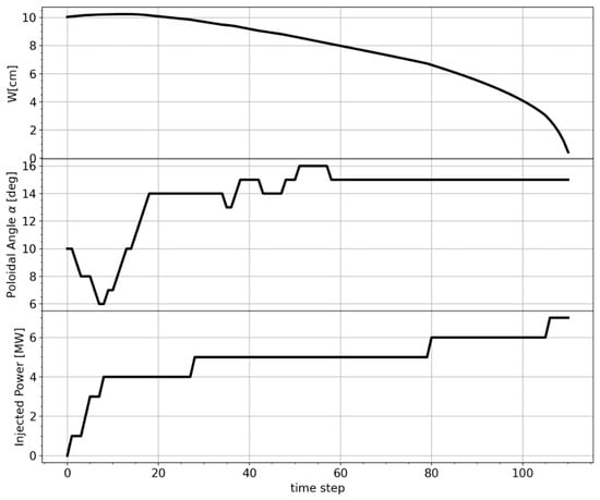
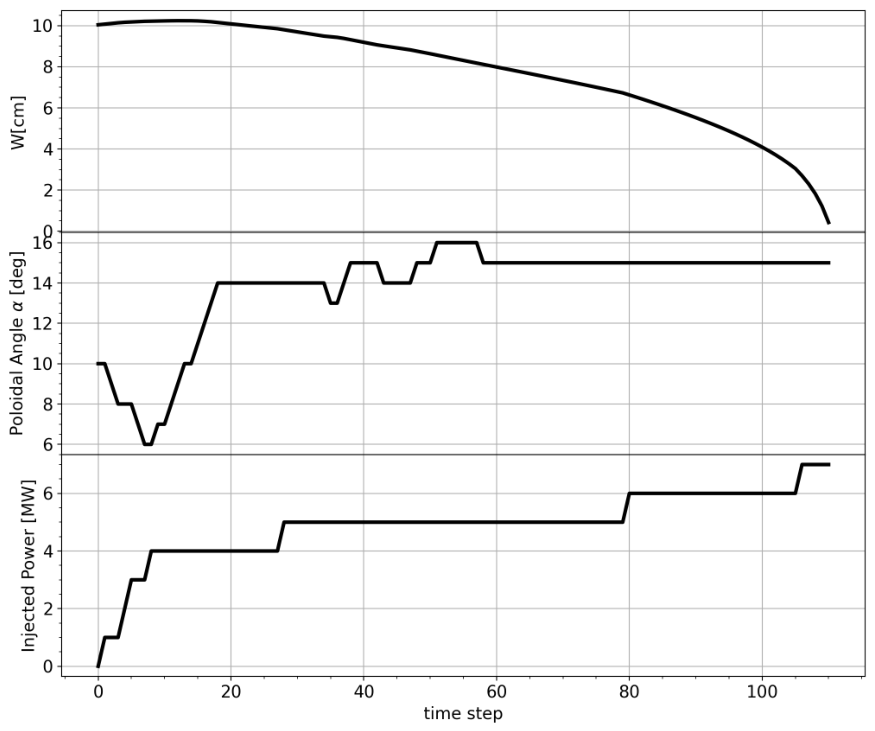
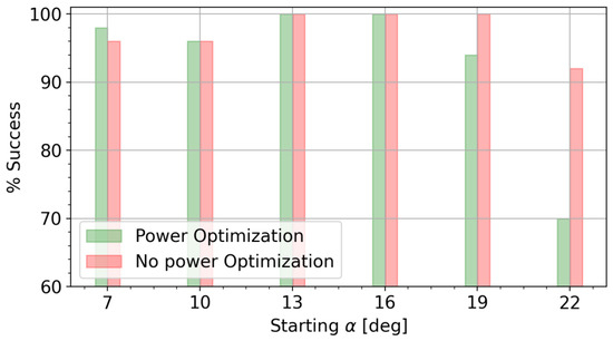
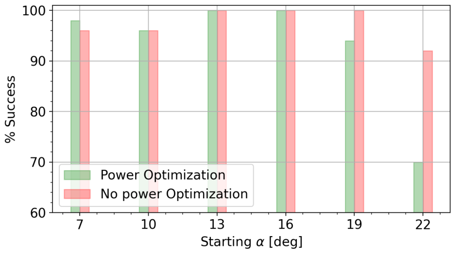
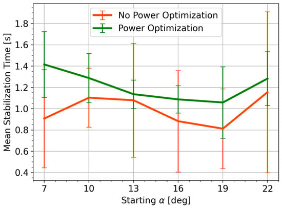
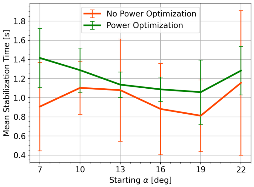
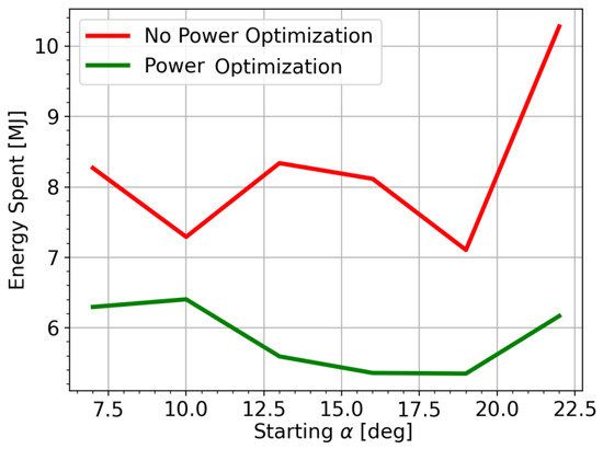
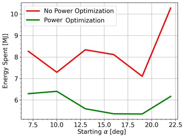
In this way, the agent was allowed to refine its strategy under the additional constraint of power minimization, without altering the underlying architecture or learning algorithm. Figure 11 illustrates a representative stabilization trajectory obtained with the reward function, including the quadratic power penalty. The simulation starts from an initial poloidal angle of 10°. The upper panel shows the evolution of the island width, which is progressively reduced until complete suppression. The middle panel reports the evolution of the launcher poloidal angle, while the lower panel displays the injected EC power. During the initial phase, the agent performs the alignment process while increasing the injected power only up to approximately 4 MW. Once the launcher approaches the optimal alignment, the power is increased further, first by 1 MW, and finally reaching the maximum level only in the final stage of the suppression process. Figure 12 compares the suppression success rate of the two policies, defined as the fraction of runs reaching complete suppression, as a function of the initial injection angle $\alpha$. The success rate is calculated on a set of 50 independent simulations. Both reach 100% at $\alpha$ = 13° and $\alpha$ = 16° and stay between 96% and 98% at the lowest angles. The policies separate for large angles. At $\alpha$ = 19°, the success rate of the power-optimized controller decreases to about 94%, while the non-optimized one still suppresses the island in every run; at $\alpha$ = 22°, the optimized policy succeeds in roughly 70% of the runs, against about 92% for the non-optimized one. For large initial angles, the policy struggles to converge to an optimal solution, which produces the drop in accuracy observed at the edge of the angular range. The cause lies in the distance from the optimal alignment: far from ${\alpha }_{opt}$, the island responds weakly to the deposited power, so the feedback driving the policy update is correspondingly weak, and the training converges more slowly. Several routes could recover this performance: extending the training, tuning the training hyperparameters, or biasing the distribution of initial angles slightly toward large values so that the agent samples the more difficult configurations more often during training. Figure 13 compares the mean stabilization time of the two policies as a function of the initial injection angle $\alpha$. Over the test interval, the power-optimized controller is slower than the non-optimized one. The longer stabilization time of the optimized controller follows from its staged power ramp-up, which keeps the injected power low during the alignment phase and delays the increase until the launcher approaches ${\alpha }_{opt}$. Figure 14 presents a comparison of the mean energy expenditure as a function of the initial poloidal angle, with and without power optimization. For each initial condition, the reported value corresponds to the average energy spent during the stabilization process. The optimized controller consistently reduces the total energy consumption across all considered starting angles. The effect is particularly pronounced for initial angles larger than 20°, where the non-optimized strategy exhibits a marked increase in energy usage, while the optimized controller maintains significantly lower values. The suppression in the optimized controller takes longer, but the lower injected power compensates for the added duration, so the total energy spent is reduced across the whole suppression trajectory. The penalty on injected power, thus, trades a modest, statistically marginal increase in stabilization time for a consistent saving in energy.

Figure 11. Trajectory of the 2/1 island width (Top), the injection angle (Middle) and the power level (Bottom) in an episode for the optimized policy.

Figure 12. Comparison between optimized (green bar) and non-optimized (red bar) agents for the success rate. The statistics are taken from an ensemble of 50 episodes where the training policy acted.

Figure 13. Comparison of suppression times between power-optimized (green) and non-optimized (red) policies. The statistics were taken from an ensemble of 50 trajectories.

Figure 14. Energy consumption for island suppression as a function of the poloidal starting angle $\alpha$. A comparison between the optimized (green line) and non-optimized network (red line).

6. Conclusions

In this work, a reinforcement-learning-based controller for magnetic island stabilization is investigated within a synthetic environment. The objective was to explore, in a controlled and interpretable setting, the potential of neural network-based strategies for the suppression of neoclassical tearing modes. The controller developed in this work is intentionally blind: it does not receive any information about the deposition location, the position of the resonant surface, or the relative alignment between launcher and island. The input state is solely represented by the magnetic island amplitude and its growth rate, implementing a kind of optimum-seeking RL-based controller. Different from ‘optimum seeking’ algorithms, different features can be performed by the architecture proposed here. The controller takes into account the limited operational angular range of the launcher, as implemented in Section 3. Further, it can also be trained to deal with power sources, as in Section 4. In Section 5, it is shown that it is possible to adopt an additional policy of saving power consumption for the training of the controller. Two control tasks were considered. In the first case, the agent was trained to perform pure angular alignment, demonstrating rapid convergence toward an optimal stabilization strategy. The network autonomously discovers effective stabilization strategies without the need for externally imposed control laws, showing a good capability to generalize the control strategy to different conditions. In particular, the network shows the capability of stabilizing a 3/2 mode (Figure 8), even if it was trained on a 2/1 dynamic. In the extended configuration, where both angular steering and power control were included, the learning process became more complex but still led to coherent stabilization behaviors. In particular, an incomplete convergence of the training process leads to a reduction in accuracy when the initial starting angle becomes larger. This is due to the reduced feedback from the island, which makes the learning process harder in that region. However, the agent was able to identify a good control sequence that allows for the full suppression of the island. The third development of the agent demonstrated the possibility of optimizing power usage within the control strategy. By introducing a quadratic cost associated with high injected power levels, the reward structure was modified so as to explicitly penalize excessive energy expenditure. As a consequence, the agent adapted its behavior, progressively biasing its strategy toward minimizing the utilized power while preserving stabilization capability. This modification resulted in a reduction in the total energy required for mode suppression, highlighting the flexibility of the reward-based framework in shaping controller behavior according to specific operational objectives. Further work is required to assess the response of the network to modifications of the environment. In particular, it will be necessary to evaluate the robustness of the learned policy with respect to perturbations such as variations in density and temperature and shifts in the resonant surface. Furthermore, we could improve the environment model used in the training loop, for instance, by including the effect of the magnetic island on transport or by training the agent on a plasma in a transient phase, such as a current ramp-down. The actuator model should likewise be made more realistic, in particular, by introducing the delay between measurement acquisition and action execution, which can alter the behavior of the agent. A suitable real-time estimator of island amplitude must also be identified, for example, from Mirnov or ECE signals, providing a quantity that scales monotonically with island width. The robustness of the policy to noise in this estimate must then be characterized, since a noisy signal can mislead the agent, an effect that becomes most severe for small islands. High-frequency diagnostic noise is mitigated by the 10 ms control step, over which it can be averaged, whereas low-frequency components survive such averaging, and their effect on the policy is left for future work.

References

- Furth, H.; Rutherford, P.; Selberg, H. Tearing mode in the cylindrical tokamak. Phys. Fluids 1973, 16, 1054–1063. [Google Scholar] [CrossRef] [Scilit]
- Gorelenkov, N.; Budny, R.; Chang, Z.; Gorelenkova, M.; Zakharov, L. A threshold for excitation of neoclassical tearing modes. Phys. Plasmas 1996, 3, 3379–3385. [Google Scholar] [CrossRef] [Scilit]
- Fitzpatrick, R. Helical temperature perturbations associated with tearing modes in tokamak plasmas. Phys. Plasmas 1995, 2, 825–838. [Google Scholar] [CrossRef] [Scilit]
- Buttery, R.; Günter, S.; Giruzzi, G.; Hender, T.; Howell, D.; Huysmans, G.; La Haye, R.; Maraschek, M.; Reimerdes, H.; Sauter, O.; et al. Neoclassical tearing modes. Plasma Phys. Control. Fusion 2000, 42, B61–B73. [Google Scholar] [CrossRef] [Scilit]
- De Vries, P.; Johnson, M.; Alper, B.; Buratti, P.; Hender, T.; Koslowski, H.; Riccardo, V.; Contributors, J.E. Survey of disruption causes at JET. Nucl. Fusion 2011, 51, 053018. [Google Scholar] [CrossRef] [Scilit]
- Lehnen, M.; Aleynikova, K.; Aleynikov, P.; Campbell, D.; Drewelow, P.; Eidietis, N.; Gasparyan, Y.; Granetz, R.; Gribov, Y.; Hartmann, N.; et al. Disruptions in ITER and strategies for their control and mitigation. J. Nucl. Mater. 2015, 463, 39–48. [Google Scholar] [CrossRef] [Scilit]
- Sauter, O.; Henderson, M.; Ramponi, G.; Zohm, H.; Zucca, C. On the requirements to control neoclassical tearing modes in burning plasmas. Plasma Phys. Control. Fusion 2010, 52, 025002. [Google Scholar] [CrossRef] [Scilit]
- Stober, J.; Barrera, L.; Behler, K.; Bock, A.; Buhler, A.; Eixenberger, H.; Giannone, L.; Kasparek, W.; Maraschek, M.; Mlynek, A.; et al. Feedback-controlled NTM stabilization on ASDEX Upgrade. In EPJ Web of Conferences; EDP Sciences: Les Ulis, France, 2015; Volume 87, p. 02017. [Google Scholar]
- Humphreys, D.; Ferron, J.; La Haye, R.; Luce, T.; Petty, C.; Prater, R.; Welander, A. Active control for stabilization of neoclassical tearing modes. Phys. Plasmas 2006, 13, 056113. [Google Scholar] [CrossRef] [Scilit]
- Seo, J.; Kim, S.; Jalalvand, A.; Choi, W.H.; Linder, B.; Kolemen, E. Avoiding fusion plasma tearing instability with deep reinforcement learning. Nature 2024, 626, 746–751. [Google Scholar] [CrossRef] [Scilit]
- Sozzi, C.; Galperti, C.; Alessi, E.; Nowak, S.; Apruzzese, G.; Belli, F.; Bin, W.; Boncagni, L.; Botrugno, A.; Bruschi, A.; et al. Experiments on magneto-hydrodynamics instabilities with ECH/ECCD in FTU using a minimal real-time control system. Nucl. Fusion 2015, 55, 083010. [Google Scholar] [CrossRef] [Scilit]
- Cha, M.; Woo, M.; Hahn, S.-H.; Park, Y.S.; Choi, M.J.; Park, J.K.; Park, B.-H.; Na, Y.S. First application of minimum island width growth rate seeking feedback controller for neoclassical tearing mode stabilization. Fusion Eng. Des. 2025, 212, 114850. [Google Scholar] [CrossRef] [Scilit]
- Kong, M.; Felici, F.; Sauter, O.; Galperti, C.; Vu, T.; Ham, C.; Hender, T.; Maraschek, M.; Reich, M.; the TCV team; et al. Physics-based control of neoclassical tearing modes on TCV. Plasma Phys. Control. Fusion 2022, 64, 044008. [Google Scholar] [CrossRef] [Scilit]
- Schulman, J.; Wolski, F.; Dhariwal, P.; Radford, A.; Klimov, O. Proximal policy optimization algorithms. arXiv 2017, arXiv:1707.06347. [Google Scholar] [CrossRef] [Scilit]
- Wilson, H. Neoclassical tearing modes. Fusion Sci. Technol. 2002, 41, 107–116. [Google Scholar]
- Salzedas, F.; Schüller, F.C.; Oomens, A.A.M.; the RTP Team. Exponentially growing tearing modes in Rijnhuizen tokamak project plasmas. Phys. Rev. Lett. 2002, 88, 075002. [Google Scholar] [CrossRef] [Scilit]
- Pucella, G.; Alessi, E.; Auriemma, F.; Buratti, P.; Falessi, M.; Giovannozzi, E.; Zonca, F.; Baruzzo, M.; Challis, C.; Dumont, R.; et al. Beta-induced Alfvén eigenmodes and geodesic acoustic modes in the presence of strong tearing activity during the current ramp-down on JET. Plasma Phys. Control. Fusion 2022, 64, 045023. [Google Scholar] [CrossRef] [Scilit]
- Puterman, M.L. Markov decision processes. Handb. Oper. Res. Manag. Sci. 1990, 2, 331–434. [Google Scholar]
- Hornik, K.; Stinchcombe, M.; White, H. Multilayer feedforward networks are universal approximators. Neural Netw. 1989, 2, 359–366. [Google Scholar] [CrossRef] [Scilit]
- Kaelbling, L.P.; Littman, M.L.; Moore, A.W. Reinforcement learning: A survey. J. Artif. Intell. Res. 1996, 4, 237–285. [Google Scholar] [CrossRef] [Scilit]
- Belousov, B.; Abdulsamad, H.; Klink, P.; Parisi, S.; Peters, J. Reinforcement Learning Algorithms: Analysis and Applications; Springer: Cham, Switzerland, 2021. [Google Scholar]
- Ambrosino, R. DTT-Divertor Tokamak Test facility: A testbed for DEMO. Fusion Eng. Des. 2021, 167, 112330. [Google Scholar] [CrossRef] [Scilit]
- Casiraghi, I.; Mantica, P.; Ambrosino, R.; Aucone, L.; Baiocchi, B.; Balbinot, L.; Barberis, T.; Castaldo, A.; Cavedon, M.; Frassinetti, L.; et al. Core integrated simulations for the Divertor Tokamak Test facility scenarios towards consistent core-pedestal-SOL modelling. Nucl. Fusion 2023, 63, 036017. [Google Scholar] [CrossRef] [Scilit]
- Farina, D. A quasi-optical beam-tracing code for electron cyclotron absorption and current drive: GRAY. Fusion Sci. Technol. 2007, 52, 154–160. [Google Scholar] [CrossRef] [Scilit]
- Rutherford, P.H. Nonlinear growth of the tearing mode. Phys. Fluids 1973, 16, 1903. [Google Scholar] [CrossRef] [Scilit]
- Lazzaro, E.; Borgogno, D.; Brunetti, D.; Comisso, L.; Fevrier, O.; Grasso, D.; Lutjens, H.; Maget, P.; Nowak, S.; Sauter, O.; et al. Physics conditions for robust control of tearing modes in a rotating tokamak plasma. Plasma Phys. Control. Fusion 2017, 60, 014044. [Google Scholar] [CrossRef] [Scilit]
- Zohm, H. Stabilization of neoclassical tearing modes by electron cyclotron current drive. Phys. Plasmas 1997, 4, 3433–3435. [Google Scholar] [CrossRef] [Scilit]
- Basiuk, V.; Huynh, P.; Merle, A.; Nowak, S.; Sauter, O.; Contributors, J.; Team, E.I. Towards self-consistent plasma modelisation in presence of neoclassical tearing mode and sawteeth: Effects on transport coefficients. Plasma Phys. Control. Fusion 2017, 59, 125012. [Google Scholar] [CrossRef] [Scilit]
- White, R.B.; Monticello, D.; Rosenbluth, M.N.; Waddell, B.V. Saturation of the Tearing Mode; Technical Report; Princeton University, Plasma Physics Laboratory: Princeton, NJ, USA, 1976. [Google Scholar] [CrossRef] [Scilit]
- Glasser, A.; Greene, J.; Johnson, J. Resistive instabilities in general toroidal plasma configurations. Phys. Fluids 1975, 18, 875–888. [Google Scholar] [CrossRef] [Scilit]
- De Lazzari, D.; Westerhof, E. On the merits of heating and current drive for tearing mode stabilization. Nucl. Fusion 2009, 49, 075002. [Google Scholar] [CrossRef] [Scilit]
- Romanelli, M.; Corrigan, G.; Parail, V.; Wiesen, S.; Ambrosino, R.; Belo, P.D.S.A.; Garzotti, L.; Harting, D.; Köchl, F.; Koskela, T.; et al. JINTRAC: A system of codes for integrated simulation of tokamak scenarios. Plasma Fusion Res. 2014, 9, 3403023. [Google Scholar] [CrossRef] [Scilit]
- Ng, A.Y.; Harada, D.; Russell, S. Policy invariance under reward transformations: Theory and application to reward shaping. In Proceedings of the ICML; Citeseer: University Park, PA, USA, 1999; Volume 99, pp. 278–287. [Google Scholar]
- Pathak, D.; Agrawal, P.; Efros, A.A.; Darrell, T. Curiosity-driven exploration by self-supervised prediction. In Proceedings of the International Conference on Machine Learning; PMLR: New York, NY, USA, 2017; pp. 2778–2787. [Google Scholar]
- Konda, V.; Tsitsiklis, J. Actor-critic algorithms. In Advances in Neural Information Processing Systems; NeurIPS Foundation: San Diego, CA, USA, 1999; Volume 12. [Google Scholar]
- Haarnoja, T.; Zhou, A.; Abbeel, P.; Levine, S. Soft actor-critic: Off-policy maximum entropy deep reinforcement learning with a stochastic actor. In Proceedings of the International Conference on Machine Learning; PMLR: New York, NY, USA, 2018; pp. 1861–1870. [Google Scholar]
- Hochreiter, S.; Schmidhuber, J. Long short-term memory. Neural Comput. 1997, 9, 1735–1780. [Google Scholar] [CrossRef] [Scilit]
- Staudemeyer, R.C.; Morris, E.R. Understanding LSTM—A tutorial into Long Short-Term Memory Recurrent Neural Networks. arXiv 2019, arXiv:1909.09586. [Google Scholar]
- Wang, H.; Zariphopoulou, T.; Zhou, X.Y. Reinforcement learning in continuous time and space: A stochastic control approach. J. Mach. Learn. Res. 2020, 21, 1–34. [Google Scholar]
Disclaimer/Publisher’s Note: The statements, opinions and data contained in all publications are solely those of the individual author(s) and contributor(s) and not of MDPI and/or the editor(s). MDPI and/or the editor(s) disclaim responsibility for any injury to people or property resulting from any ideas, methods, instructions or products referred to in the content. |
© 2026 by the authors. Licensee MDPI, Basel, Switzerland. This article is an open access article distributed under the terms and conditions of the Creative Commons Attribution (CC BY) license.