Hemolysis in Pulsed Field Ablation: A Mathematical–Physical Model

Abstract

Pulsed Field Ablation (PFA) is an emerging technique for the treatment of cardiac arrhythmias based on the irreversible electroporation of cardiomyocytes. It is rapidly replacing conventional thermal ablation owing to its tissue selectivity. However, its widespread clinical adoption has also highlighted several procedure-related complications. Although PFA is generally regarded as tissue-selective, increasing evidence indicates that exposing circulating blood to intense electric fields may induce red blood cell (RBC) damage and hemolysis. In this work, we develop a physics-based mathematical model to predict the extent of hemolysis during PFA procedures. The model combines a simplified representation of the electric field generated by a bipolar PFA catheter with experimentally derived hemolysis–response relationships, allowing the volume of damaged blood and free hemoglobin (fHb) release to be predicted as functions of pulse amplitude, pulse number, and device geometry. The proposed framework is consistent with both classical electroporation theory and recent clinical observations reporting a dose-dependent increase in hemolysis following PFA. The results provide a mechanistic interpretation of blood damage during PFA. Despite several simplifying assumptions, the proposed framework yields a quantitative tool for assessing hemolytic risk and may support the optimization of future PFA protocols.

1. Introduction

Pulsed Field Ablation (PFA) has recently emerged as a promising alternative to conventional radiofrequency and cryoablation for the treatment of atrial fibrillation (AF) (see [1,2]). Its mechanism of action relies on the delivery of short high-voltage electrical pulses that induce irreversible electroporation of cardiomyocytes while largely preserving surrounding tissues. The applied electric field creates permanent nano-scale pores in cell membranes, causing cell death, a phenomenon known as irreversible electroporation (IRE) (see, e.g., [3,4,5,6]). Most authors claim that PFA operates on the basis of tissue selectivity (see, e.g., [7] and references therein). This means that the electric field is optimized to target cardiac tissue (cardiomyocytes) while sparing adjacent structures such as the esophagus, vasculature, and phrenic nerve, thereby reducing the risk of collateral damage. However, some recent publications (see [8,9,10,11,12,13]) have pointed out that various complications may arise. For instance, Joule heating may increase the local tissue temperature well above physiological levels, potentially leading to irreversible injury of adjacent critical structures such as the esophageal wall. Moreover, electric fields may activate platelets, leading to blood coagulation. Hemolysis has also emerged as a potential complication and has been associated with acute kidney injury [14]. In fact, exposure of circulating blood to strong electric fields may also damage red blood cells (RBCs). Experimental evidence dating back to classical electroporation studies has shown that erythrocytes undergo membrane permeabilization and eventual lysis when subjected to transient electric fields [15,16,17]. Recent clinical studies have confirmed that hemolysis is frequently observed after PFA procedures, with measurable increases in plasma free hemoglobin (fHb) and related biomarkers in a large fraction of patients [18,19,20]. The extent of hemolysis appears to be correlated with pulse number and delivered energy, suggesting a cumulative damage mechanism [21].

From a mechanistic perspective, RBC injuries result from a complex interplay between electroporation, membrane resealing dynamics, and hydrodynamic stresses [22,23]. However, current models (see, e.g., [18,19,24,25,26]) remain largely empirical and do not encompass the coupled effects of electric fields, flow transport, and biological heterogeneity. It should be remarked that hemolysis (or RBC damage more generally [27]) due primarily to mechanical–chemical failure of the membrane is a complex phenomenon to describe (see [28,29,30,31,32,33,34,35]). Indeed, RBCs are essentially fluid-filled sacs enclosed by a thin and flexible membrane supported by a cytoskeletal network, allowing the large deformations needed to pass through narrow capillaries. As a consequence, there are several processes that can lead to the death of a red blood cell, including mechanical stress (shear forces stretching the membrane), osmotic imbalance leading to an increase in intracellular pressure until membrane rupture, and thermal or chemical disruption.

Recent meta-analyses have confirmed that PFA provides efficacy and safety broadly comparable to that of conventional ablation modalities, with potential advantages in AF burden reduction and procedural efficiency, while also showing that early post-PFA atrial tachyarrhythmia recurrences are strongly predictive of late recurrence (see [36]). Against this broader clinical background, increasing attention is being directed towards procedure-related complications, including PFA-induced hemolysis (see [37,38]). In [39], the authors identified PFA-induced hemolysis as a clinically relevant device- and dose-dependent adverse effect. However, they did not provide a quantitative mechanistic framework linking electric field exposure, catheter geometry, and pulse number to the resulting volume of damaged blood and free hemoglobin release.

The main objective of the present work is to develop a mathematical–physical model for PFA-induced hemolysis in order to provide quantitative predictions about its occurrence. More precisely, we investigate the electric field generated by a typical device used in PFA procedures for the treatment of atrial fibrillation. The electric field is produced by a generator and delivered via catheter, which can be shaped into a basket or flower configuration. There are several commercialized devices with different technical parameters; here, we mostly refer to Farapulse (by Boston Scientific), as already done in our other work [9]. The applied pulses are bipolar, meaning that they are generated between electrodes on the catheter; thus, its action is confined to the vicinity of the targeted tissue. The biphasic nature (pulses of alternate polarity) is designed to improve efficiency. The system delivers short high-voltage pulses up to 2.0 kV. These pulses create nanopores in the membranes of cardiomyocytes, leading to irreversible cell injury and cell death, thereby eliminating the source of ectopic heart stimuli.

Our model is consistent with both classical electroporation theory (see [4,16]) and recent clinical observations in PFA (see [18,19]), and explains the dependence of hemolysis on pulse number and energy delivery [21]. However, it has several limitations. First, the geometrical setting has been simplified in order to reduce the computational complexity. Second, the model validation is based on representative experimental trends rather than direct quantitative datasets. While the model captures key qualitative behaviors, systematic experimental validation will be required for quantitative predictions. Despite these limitations, the proposed framework provides a mechanistic foundation for understanding hemolysis in PFA and offers a flexible basis for future developments.

The rest of the paper is organized as follows: Section 2 presents the mathematical–physical framework developed in this work; in Section 2.1, we present a simplified model of the electric field generated by a typical PFA ablator; in Section 2.2, we identify a criterion for the occurrence of hemolysis following the studies reported in [15,16,40] concerning the dielectric breakdown of RBCs; in Section 2.3, we discuss the relationship between membrane poration, resealing, and Hb release; in Section 2.4 and Section 2.5, we provide an estimate of the hemolyzed volume, first from a general perspective and then specifically for a PFA session; Section 3 is devoted to a comparison between model predictions and data available in the literature; finally, Section 4 presents some concluding remarks, while most of the mathematical details are confined to Appendix A.1.

2. Methods

2.1. Electric Field Distribution in the PFA Framework

The physical regime relevant to PFA is quasi-static. Let us define $t_p$ as the characteristic pulse duration, c as the speed of light, and d as the characteristic length of the physical device. For the reader’s convenience, Table 1 lists the most relevant physical parameters together with their dimensions and typical values in the present context.

Table 1. List of parameters, dimensions in SI units, and typical values in the PFA context.

Parameter	Meaning	Unit	SI Dimension	Value
$\mathcal{V}$	applied voltage	V	$\left[\mathrm{k}\mathrm{g}{\mathrm{m}}^2{\mathrm{A}}^{-1}{\mathrm{s}}^{-3}\right]$	$(1.8$–$2.2) \times {10}^3$
$\varphi$	hematocrit	% (in volume)	[−]	40–50
$v_{\mathrm{RBC}}$	mean RBC volume	fL	$\left[{\mathrm{m}}^3\right]$	$9\times {10}^{-17}$
$t_p$	pulse duration	s	[s]	(0.5–1)$\times {10}^{-4}$
${\tau }_p$	pulse-train period	s	[s]	$0.5$
${\tau }_b$	heartbeat period	s	[s]	$\approx 1$
c	light speed	$\mathrm{m}{\mathrm{s}}^{-1}$	[$\mathrm{m}{\mathrm{s}}^{-1}$]	$\approx 3\times {10}^8$
d	dipole length	m	[m]	(0.8–1)$\times {10}^{-3}$
${\epsilon }_0$	vacuum permittivity	F/m	[${\mathrm{kg}}^{-1}{\mathrm{m}}^{-3}{\mathrm{s}}^4{\mathrm{A}}^2]$	$\approx 8.85\times {10}^{-12}$
${\epsilon }_r$	blood permittivity	—	$[-]$	≈(5–7)$\times {10}^3$
$\sigma$	electric conductivity	$\mathrm{S}{\mathrm{m}}^{-1}$	[$\mathrm{k}{\mathrm{g}}^{-1}{\mathrm{m}}^{-3}{\mathrm{s}}^3{\mathrm{A}}^2$]	≈0.7

Since $t_p=\mathcal{O}\left({10}^{-4}\mathrm{s}\right)$ and $d=\mathcal{O}\left({10}^{-3}\mathrm{m}\right)$ (see, e.g., [9]), we have

$${\displaystyle \frac{\omega }{c}}d\ll 1,$$

(1)

where $\omega =2\pi /t_p$. In order to establish that we may consider the electric field to be quasi-static, we regard a single pulse of duration $t_p$ as part of a sequence of pulses having the same period. This kind of sequence would generate a wave of length $\lambda =2\pi c/\omega$. The condition under which the electric field is quasi-static is $d\ll \lambda$, which is largely fulfilled because of (1). Therefore, propagation and retardation effects are negligible and the electric field can be described using a quasi-static approximation. However, quasi-static does not mean purely electrostatic, since a major role in PFA is played by the dipolar current. This current destabilizes the lipid structure of the cell membrane (which behaves as a dielectric) until pores are created, leading to cell death.

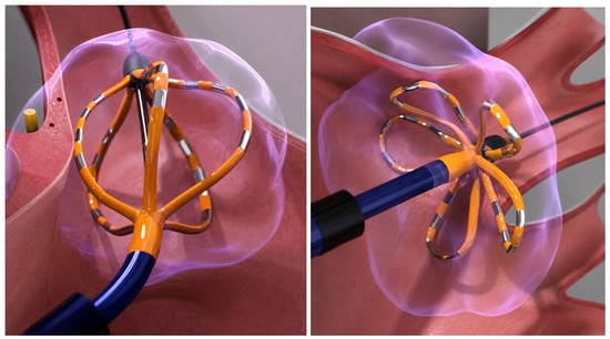
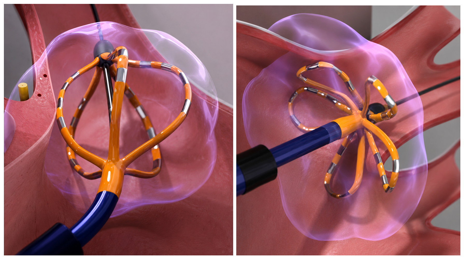
The real devices used in a PFA session possess complex geometry. One of the most common, Farapulse by Boston Scientific, consists of five splines, each carrying four electrodes separated by an insulator. The device can be set in two different configurations, “basket” and “flower” (see Figure 1), both of which are used during a complete clinical treatment.

Figure 1. Basket (left panel) and flower (right panel) configurations of the Farapulse ablator (schematic illustration generated with the assistance of OpenAI ChatGPT (GPT-5.5)).

For the purposes of the present paper, we model the two electrodes as a pair of charged conducting spheres. This choice allows for representation of both the field potential and the electric field. Appendix A.1 reports the technical details.

Let d be a reference length scale and $(x,y,z)$ a Cartesian orthogonal reference frame. The two spheres have radius $a=d/4$ and their centers are placed at $(\pm 3d/4,0,0)$, respectively. The two spheres are kept at potential

$${\Phi }_{\mathrm{left}}=+{\displaystyle \frac{\mathcal{V}}{2}},{\Phi }_{\mathrm{right}}=-{\displaystyle \frac{\mathcal{V}}{2}}.$$

(2)

Therefore, the voltage difference between the two metallic spheres is $\mathcal{V}$. Since the potentials of the two conductors are prescribed, in the quasi-static approximation the electric field is obtained from the electrostatic potential as

$$\mathit{E}=-\nabla \Phi .$$

(3)

We now suppose that the two metallic spheres are immersed in a homogeneous and isotropic biological tissue with constant and uniform electrical conductivity $\sigma$. A typical value is $\sigma \simeq 0.7\mathrm{S}{\mathrm{m}}^{-1}$ (see [41,42]). In a conductive medium, the current density is related to the electric field by Ohm’s law $\mathit{J}=\sigma \mathit{E}.$ In the quasi-static regime, if the conductivity is uniform, charge conservation gives $\nabla ·\mathit{J}=0.$ Since $\mathit{J}=\sigma \mathit{E}=-\sigma \nabla \Phi$, the function $\Phi$ satisfies Laplace’s equation outside the two spheres:

$${\nabla }^2\Phi =0.$$

(4)

The dielectric permittivity ${\epsilon }_r{\epsilon }_0$ of blood does not appear explicitly in $\mathit{E}$ when the boundary conditions are imposed, instead determining the amount of charge induced on the conductors. In summary, the electric field is controlled by the imposed voltage and by the geometry, while the current density is obtained by multiplying the field by the tissue conductivity.

Equation (4) with the boundary conditions in (2) can be solved explicitly using bi-spherical coordinates [43] (the reader is referred to Appendix A.6 for details). For the purposes of the present paper, we use only the average $\overline{E}$ of $\left|\mathit{E}\right|$ over the full solid angle at fixed r, that is,

$$\overline{E}\left(r\right)={\displaystyle \frac{1}{4\pi }}{\int }_{4\pi }\left|\mathit{E}(r,\theta ,\varphi )\right|d\Omega .$$

(5)

A power series expansion of (5) in $d/r$ yields

$$\overline{E}\left(r\right)={\displaystyle \frac{\left|\mathcal{V}\right|}{d}}\left[C_1{\left({\displaystyle \frac{d}{r}}\right)}^3+C_3{\left({\displaystyle \frac{d}{r}}\right)}^5+O\left({\displaystyle \frac{d^7}{r^7}}\right)\right],$$

(6)

with $C_1\simeq 0.31$ and $C_3\simeq -0.040$. The leading approximation is

$$\overline{E}\left(r\right)\simeq 0.31{\displaystyle \frac{\left|\mathcal{V}\right|d^2}{r^3}}.$$

(7)

We remark that the maximum estimated relative error ${\Delta }_{\max }$ is obtained at $r=d$, that is, ${\Delta }_{\max }\simeq 0.13.$

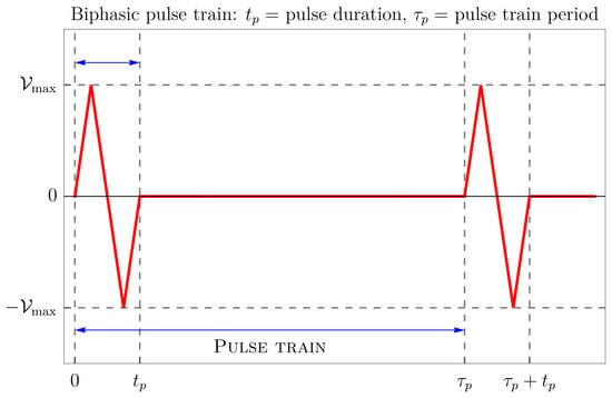
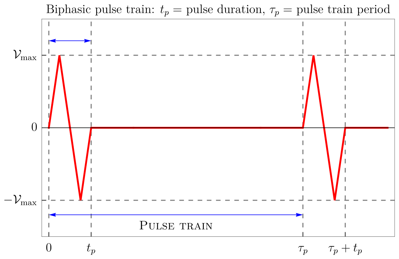
Now, focusing only on a single individual pulse train (see Figure 2), we can write

$$\mathcal{V}\left(t\right)=\left\{\begin{array}{cc}{\mathcal{V}}_{\max }\sin \left(\omega t\right),\hfill & 0\le t\le t_p,\hfill \\ \hfill & \\ 0,\hfill & t_p<t\le {\tau }_p\hfill \end{array}\right.$$

with

$$\omega ={\displaystyle \frac{2\pi }{t_p}}.$$

(8)

Recalling (7), we have

$$\overline{E}\left({\displaystyle \frac{r}{d}}\right)\simeq 0.31{\displaystyle \frac{{\mathcal{V}}_{\max }}{d}}{\left({\displaystyle \frac{r}{d}}\right)}^{-3}.$$

(9)

Figure 2. Schematic representation of a possible biphasic pulse train (the waveform shown is illustrative; in the mathematical model, the elementary pulse is represented by a sinusoidal waveform). The pulse train period is ${\tau }_p$. Note that the electrical pulse has a duration $t_p$ which is significantly less than the period ${\tau }_p$ with which the pulse train is repeated. In the present paper, we set ${\tau }_p\approx 0.5\mathrm{s}$, while $t_p$ ranges between $5\times {10}^{-5}\mathrm{s}$ and ${10}^{-4}$ s.

Note that the real geometry can only be roughly simulated by a pair of charged spheres. A reasonable approximation is to assume that the volume of the electrodes–insulator system equals the volume of a sphere of radius d which contains the two metallic spheres representing a single pair of ablator electrodes. In other words, if ${\mathfrak{V}}_{\mathrm{device}}$ is the volume of the device (a pair of metal pins separated by an insulating cylinder), then $d=\sqrt[3]{3{\mathfrak{V}}_{\mathrm{device}})/\left(4\pi \right)}$. This is because we treat the sphere of radius d which encloses the two metallic spheres as impermeable to blood, in analogy with the electrode–insulator assembly, i.e., the region from which blood is excluded. Specifically, using typical characteristic data of the elementary Farapulse electrode–insulator–electrode element, we find $d\simeq 0.9$ mm.

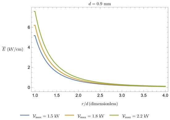
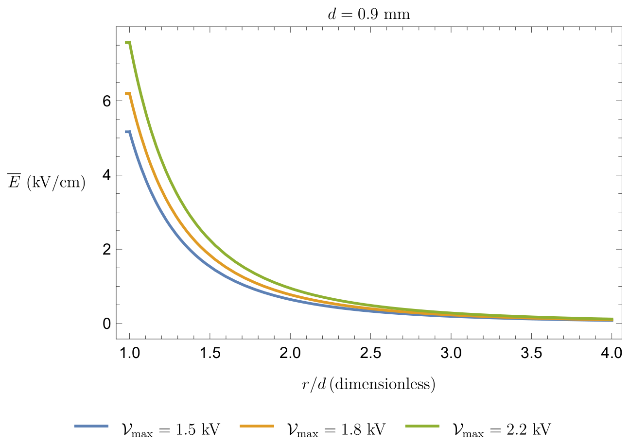
Formula (9) is sufficiently accurate only for $r\ge d$, that is, the region available to blood. In any case, we are interested in calculating the volume in which $\overline{E}$ exceeds some threshold value; if this happens for distances on the order of d, then it will be certainly true for $r<d$. Figure 3 shows the behavior of $\overline{E}\left(\xi \right)$ for $\xi =r/d>1$.

Figure 3. Mean electric field intensity $\overline{E}\left(\xi \right)$ (in kV/cm) as a function of the normalized distance $\xi =r/d$ for $\xi \ge 1$ and $d=0.9$ mm for some typical values of ${\mathcal{V}}_{\max }$ (in kV).

2.2. Hemolysis Dynamics

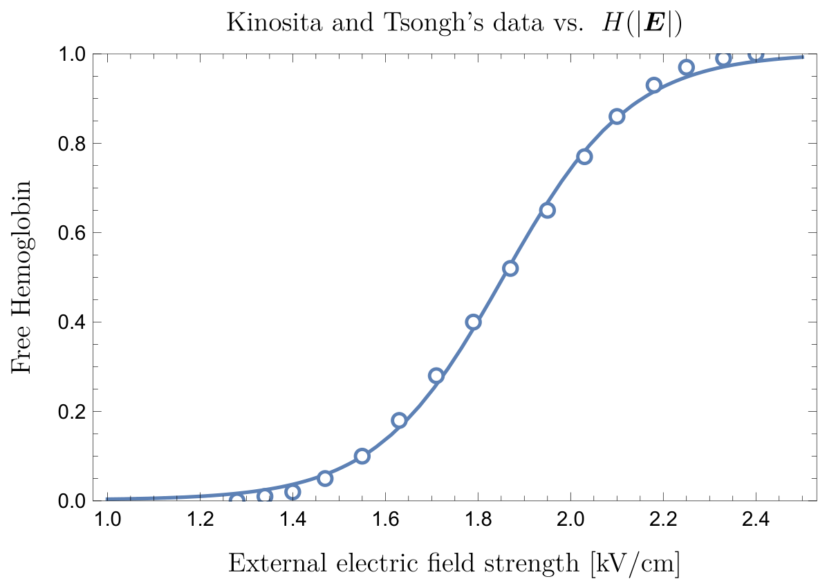
To identify a criterion for the occurrence of hemolysis, we follow [15,16,40], which investigated dielectric breakdown of cell membranes in RBCs and bacteria under applied electric fields. RBC damage is usually monitored through the release of Hb or other specific biomarkers (for example potassium) in the supernatant. The key finding from these studies is that the relationship between hemolysis and electric field strength follows a sigmoidal curve, indicating a threshold-like process. In particular, the onset of hemolysis occurs when the applied electric field is larger than $E_{\mathrm{lys}}$. This value can be estimated (see [44]) to be on the order of 1–2 kV/cm. However, this value depends on the cell orientation and shape as well as the duration of the electric field application, denoted as $t_A$.

We remark that in a general context the peak field, pulse duration, transferred charge, and pulse train structure are not interchangeable quantities; however, in the framework established in [15,16], damage to RBCs is primarily determined by two combined conditions: the electric field magnitude must exceed a critical threshold, and it must remain above that threshold for a sufficiently long exposure time. Thus, the relevant exposure measure is not the total transferred charge or the waveform but the intensity of the electric field.

In a constant and uniform electric field $\mathit{E}$ applied for a time interval $t_A$, a simple analytical model for the density $n_{\mathrm{dam}}\left(t\right)$ of damaged RBCs per unit volume at time $t\le t_A$ is

$$n_{\mathrm{dam}}\left(t\right)=n_{0}H\left(\left|\mathit{E}\right|,t,t_A\right),$$

(10)

where $n_0$ is the total RBC density (note that $n_0$ is linked to the hematocrit $\varphi$ through $n_0=\varphi /v_{\mathrm{RBC}}$, with $v_{\mathrm{RBC}}$ the average volume of a single RBC), i.e., number of RBCs per unit volume, and (see [45])

$$H\left(\left|\mathit{E}\right|,t,t_A\right)={\displaystyle \frac{1}{2}}\left[1+tanh\left({\displaystyle \frac{\left|\mathit{E}\right|-E_{50}\left(t_A\right)}{\delta \left(t_A\right)}}\right)\right]\left(1-e^{-t/{\tau }_{\mathrm{m}}}\right),$$

(11)

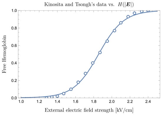
where $E_{50}$ is the value corresponding to 50% hemolysis and $\delta \left(t_A\right)$ is the width of the transition region. Figure 4 shows both the data in [40] and their fit through a function of type (11) for $t\gg {\tau }_{\mathrm{m}}$.

Figure 4. Reproduction of Figure 4a in [40]. A nonlinear fitting procedure shows that the data from Kinosita and Tsong can be simulated by (11) with $E_{50}\left(t_A\right)\approx 1.85$ kV/cm, $\delta \left(t_A\right)\approx 0.27$ kV/cm, and $t\gg {\tau }_{\mathrm{m}}$.

The experiments in [15,16,26,40] showed that both $E_{50}$ and the transition width $\delta$ depend on $t_A$. Model (11) assumes that damage does not occur instantaneously, meaning that the number of damaged cells per unit volume caused by a field of intensity $\left|\mathit{E}\right|$ is reached along a time ${\tau }_{\mathrm{m}}$. The characteristic time ${\tau }_{\mathrm{m}}$ corresponds to the membrane charging time constant. Its value can be estimated in the range $0.1–1\mathsf{\mu }\mathrm{s}$ (see, e.g., [15,16,40]), while the time t we are interested in is on the same order of $t_p$, that is, $50–100\mathsf{\mu }\mathrm{s}.$ Therefore, the exponential term in (11) can be safely neglected, meaning that each RBC membrane is damaged almost instantaneously. Concerning $E_{50}\left(t_A\right)$ and $\delta \left(t_A\right)$, we refer to [40]. In particular, Figure 4a in [40] shows that the hemolysis occurs at ∼1 kV/cm; however, 50% hemolysis is observed only at about 1.8 kV/cm, and saturation occurs above 2.5 kV/cm. We note that $\delta$ is small enough to make the transition from no hemolysis to full hemolysis a rather sharp one.

In addition, Kinosita and Tsong in [17] carried out fundamental experimental studies providing quantitative relationships between the intensity of the applied electric field and damage to RBCs.

Within the context of PFA, the pulse duration $t_A$ is nothing but $t_p$, and the order of magnitude of the pulse duration in the experiment in [15,40] is on the same order as that used in standard PFA protocols. However, the experimental setting used by the authors is somehow different from typical PFA conditions. Therefore, the consistency of the model must be assessed a posteriori based on the amount of fHb predicted by our model and that measured after a real PFA procedure.

For a biphasic electric field, (11) must be modified to account for the irreversibility of membrane breakdown. Thus, the relevant variable is the maximum electric field intensity $\mathit{E}$, i.e., $\overline{E}\left(r\right)$, as given by (9). Hence, assuming that there are no damaged cells at time $t=0$, the local density of damaged cells in one time period $t_p$ is

$$n_{\mathrm{dam}}\left(r\right)=n_{0}H\left(\overline{E}\left(r\right)\right),$$

(12)

where H is given by (11), dropping the exponential term.

To assess the effect of the radial-mean approximation, we performed a numerical comparison between

$$H\left(\overline{E}\left(r\right)\right)\mathrm{and}\overline{H}\left(r\right)={\displaystyle \frac{1}{4\pi }}{\int }_{4\pi }H\left(\left|\mathbf{E}\right(r,\theta ,\varphi \left)\right|\right)d\Omega ,$$

since the electric field is available in analytical form (see Appendix A.5). This allows the angular average of the nonlinear response to be evaluated directly. The test showed that the difference between the two formulations is negligible and results in no significant change in the estimated damaged volume, confirming that the radial-mean field approximation is adequate for the present geometric model.

2.3. Hb Release and RBC Resealing: How Are They Connected?

When the intensity of the electric field exceeds $E_{\mathrm{lys}}$, poration of the RBC’s membrane begins. However, poration may be non-uniform, meaning that some pores may not be large enough to allow for complete Hb release. Membrane resealing may occur if the pulses are sufficiently separated in time, thereby reducing the damage. In other words, neglecting the recovery effect may lead to overestimation of the final amount of Hb released.

Resealing has been investigated by Saulis et al. [22], who showed that it is a multiscale process. Once the electric field is removed, pore dimension reduces more or less with an exponential time decay, with the relevant interval ranging from less than 1 s to more than 1 h. This aspect should be taken into account in interpretation. For example, to correctly interpret the work of Kinosita and Tsong [17], where their sigmoids represent the damage that escapes resealing, the resealing time scale of interest in PFA needs to be on the order of one second, since two subsequent pulses are separated by a time interval having the same order of magnitude. The work of Saulis et al. suggests that part of the damage induced by the electric field decays rather rapidly once the device is switched off.

A natural question following from this is how small the pores must be in order to prevent Hb release. The Hb diameter $D_{\mathrm{Hb}}\approx 5.5$ nm, so an Hb molecule can escape only if the pore radius $r_p\gtrsim 2.75$ nm. Unfortunately, it seems that there are no experimental data directly measuring Hb release after a single pulse of electroporation of erythrocytes with a temporal resolution sufficient to evaluate the time over which the pores remain permeable to Hb. The pioneering study by Kinosita and Tsong suggests that Hb is not released directly through electroporation-induced membrane pores; rather, the pores initially allow for ionic transport, resulting in osmotic imbalance that causes cell swelling, and ultimately in colloidal hemolysis of the erythrocyte. Clinical studies on PFA [18,26,46] typically measure fHb either immediately after the procedure or 24 h later, rather than at the millisecond or second timescales required to characterize the kinetics of hemoglobin release.

2.4. Estimate of Hemolyzed Blood in a Sample of Volume

We now examine a volume $\mathfrak{V}$ of blood exposed to the electric field (9) with the aim of estimating the volume of damaged blood ${\mathfrak{V}}_{\mathrm{dam}}$. We assume that the middle point of the dipole is located at the origin of the reference frame and sufficiently far from the boundary of $\mathfrak{V}$. We also assume that the density $n_0$ is uniform in the volume $\mathfrak{V}$. For the purpose of estimating the volume of hemolyzed blood, what matters is the mean field intensity during a single pulse at a distance r from the dipole, namely, $\overline{E}$, given by (9). The local density of damaged RBCs in a period is given by (12), and the corresponding local fraction is $H\left(\overline{E}\left(r\right)\right).$ Therefore, an effective measure of ${\mathfrak{V}}_{\mathrm{dam}}$ in one time period is obtained by spatial averaging:

$${\mathfrak{V}}_{\mathrm{dam}}=\mathfrak{V}{F}_{\mathrm{dam}},\mathrm{with}{F}_{\mathrm{dam}}={\displaystyle \frac{1}{\mathfrak{V}}}{\int }_{\mathfrak{V}}H\left(\overline{E}\left(r\right)\right)d\mathit{x}.$$

(13)

Assuming, for example, that $\mathfrak{V}$ is a sphere of radius R centered at the origin and excluding a core with diameter d, we have

$$F_{\mathrm{dam}}\left(R\right)={\displaystyle \frac{3}{R^3}}{\int }_d^{R}H\left(\overline{E}\left(r\right)\right)r^{2}dr,$$

(14)

or equivalently,

$$F_{\mathrm{dam}}\left({\displaystyle \frac{R}{d}}\right)={\displaystyle \frac{3d^3}{R^3}}{\int }_1^{R/d}H\left(\overline{E}\left(d\xi \right)\right){\xi }^{2}d\xi .$$

(15)

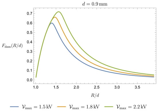
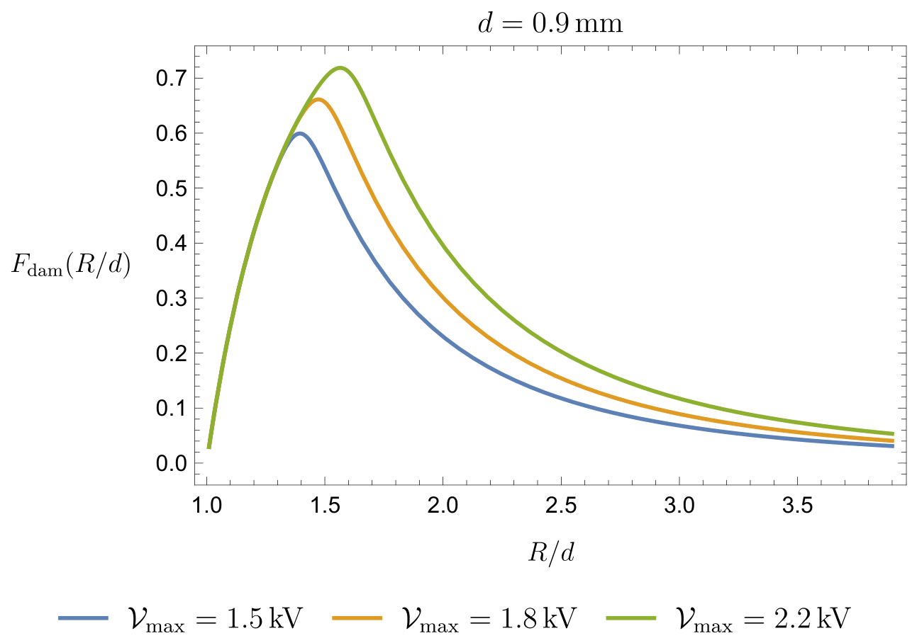
The function $F_{\mathrm{dam}}$ is shown in Figure 5.

Figure 5. Fraction of damaged blood as a function of $R/d$ for $E_{50}\approx 1.85$ kV/cm and $\delta =0.27$ kV/cm.

Thus, using (13)–(15), we find that the volume of damaged blood is given by

$${\mathfrak{V}}_{\mathrm{dam}}=4\pi d^3{\int }_1^{R/d}H\left(\overline{E}\left(d\xi \right)\right){\xi }^{2}d\xi .$$

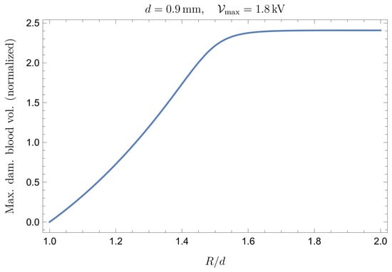
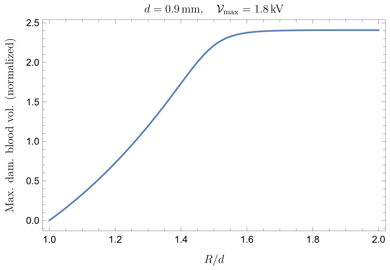
In Figure 6, we show the volume ${\mathfrak{V}}_{\mathrm{dam}}$, normalized with respect to the volume of the sphere of radius d (the sphere which is not accessible to blood) as a function of $R/d$, i.e.,

$${\displaystyle \frac{{\mathfrak{V}}_{\mathrm{dam}}\left(R/d\right)}{4/3\pi d^3}}=3{\int }_1^{R/d}H\left(\overline{E}\left(d\xi \right)\right){\xi }^{2}d\xi .$$

Figure 6. Volume ${\mathfrak{V}}_{\mathrm{dam}}$ normalized with respect to the volume of the sphere of radius d (the sphere which is not accessible to blood) as a function of $R/d$ for ${\mathcal{V}}_{\max }=1.8$ kV.

As expected, when R becomes much larger than d, the normalized volume approaches an asymptotic value.

It is worth emphasizing that Equation (13)may be misleading if interpreted superficially, as it could suggest that the hemolyzed blood volume is simply proportional to the total volume $\mathfrak{V}$. This is not the case; the relevant contribution comes only from the portion of blood sufficiently close to the dipole, where the electric field exceeds the threshold value $E_{50}$. Therefore, ${\mathfrak{V}}_{\mathrm{dam}}$ may coincide with $\mathfrak{V}$ only when $\mathfrak{V}$ is sufficiently small, so that the electric field intensity remains above $E_{50}$ throughout the entire volume. Conversely, when $\mathfrak{V}$ is very large, the dipole field becomes negligible within most of the volume, and ${\mathfrak{V}}_{\mathrm{dam}}$ approaches an asymptotic value. This limiting value corresponds in practice to the spatial region in which $\overline{E}>E_{50}$.

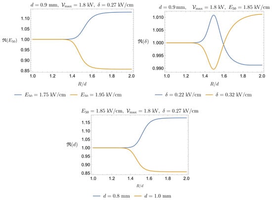
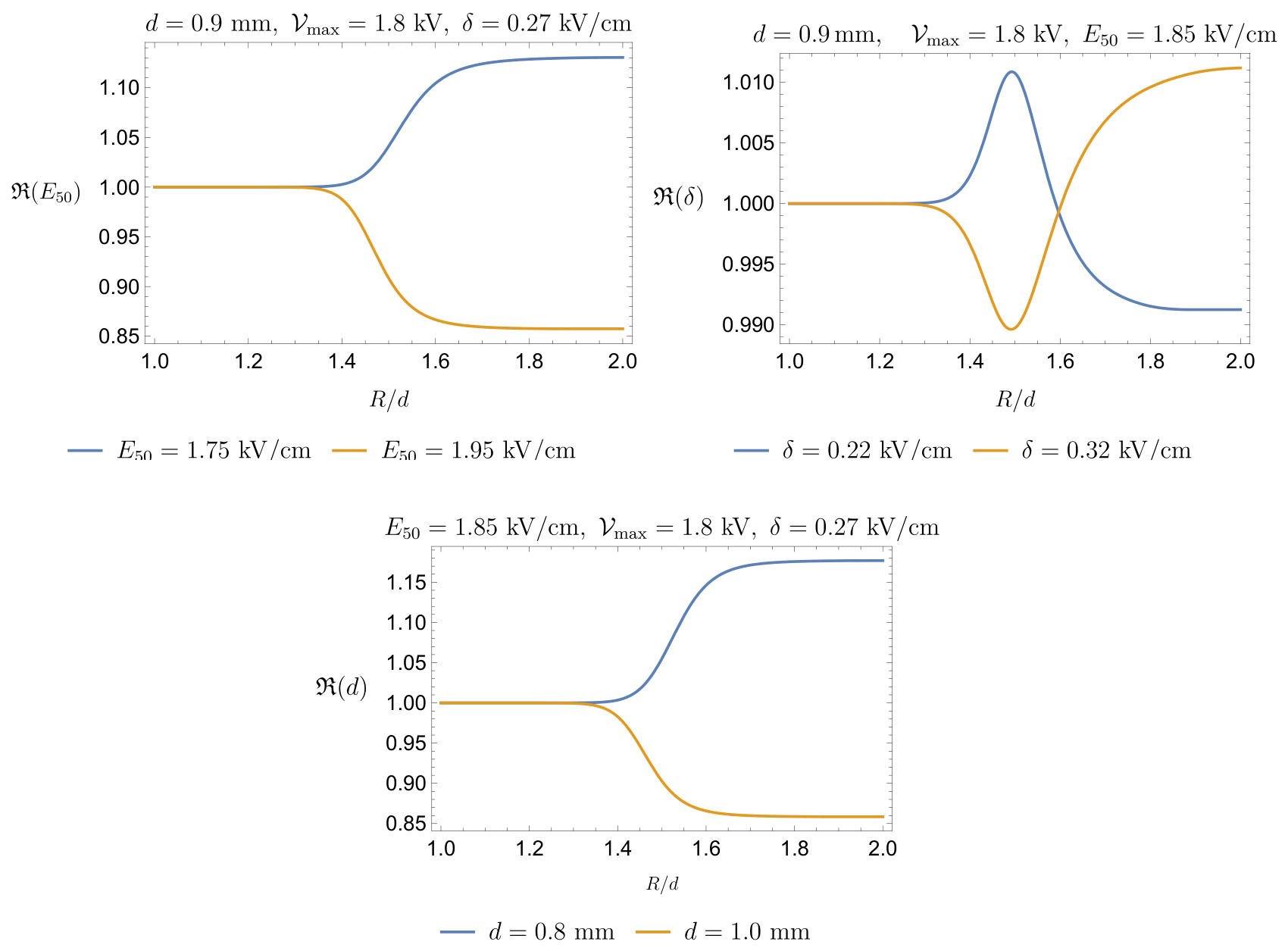
Figure 6 is based on the assumptions that $d=0.9$ mm, $E_{50}\approx 1.85$ kV/cm, and $\delta \approx 0.27$ kV/cm (see Figure 4). Since these parameter values are subsequently used to estimate the expected amount of fHb released during a standard PFA clinical treatment, it is natural to assess the sensitivity of ${\mathfrak{V}}_{\mathrm{dam}}$ to their variation. To this end, we define ${\mathfrak{V}}_{\mathrm{dam},\mathrm{ref}}$ as the function shown in Figure 6 and introduce the following ratios.

$$\mathfrak{R}\left(E_{50}\right)={\displaystyle \frac{{\mathfrak{V}}_{\mathrm{dam}}\left(E_{50}\right)}{{\mathfrak{V}}_{\mathrm{dam},\mathrm{ref}}}}\mathfrak{R}\left(\delta \right)={\displaystyle \frac{{\mathfrak{V}}_{\mathrm{dam}}\left(\delta \right)}{{\mathfrak{V}}_{\mathrm{dam},\mathrm{ref}}}}\mathfrak{R}\left(d\right)={\displaystyle \frac{{\mathfrak{V}}_{\mathrm{dam}}\left(d\right)}{{\mathfrak{V}}_{\mathrm{dam},\mathrm{ref}}}}$$

(16)

For each ratio, one parameter is varied while the other two are kept fixed. Figure 7 illustrates the behavior of the functions in (16) with respect to $R/d$. The sensitivity analysis indicates that the predicted volume of damaged blood is relatively robust with respect to the three parameters considered here. The model shows a moderate sensitivity to $E_{50}$ and d, with variations of ${\mathfrak{V}}_{\mathrm{dam}}$ remaining below approximately 15%, whereas the dependence on $\delta$ is negligible, with variations below 1%. Therefore, the uncertainty associated with the precise choice of these parameters does not substantially affect the predicted order of magnitude of the damaged blood volume. Additionally, the markedly different sensitivities to $E_{50}$ and $\delta$ indicate that the predicted volume of damaged blood is primarily controlled by the characteristic field threshold for hemolysis, whereas the precise width of the transition region has a negligible effect on the final estimate.

Figure 7. Upper Left Panel: Sensitivity of ${\mathfrak{V}}_{\mathrm{dam}}$ to $E_{50}$; the influence of $E_{50}$ does not exceed 15%. Upper Right Panel: Sensitivity of ${\mathfrak{V}}_{\mathrm{dam}}$ to $\delta$; the influence of $\delta$ remains within 1%. Lower Panel: Sensitivity of ${\mathfrak{V}}_{\mathrm{dam}}$ to d; its influence is very similar to that of $E_{50}$ and remains below 15%.

2.5. Estimate of Hemolyzed Blood in a PFA Application

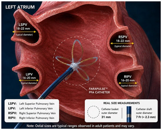
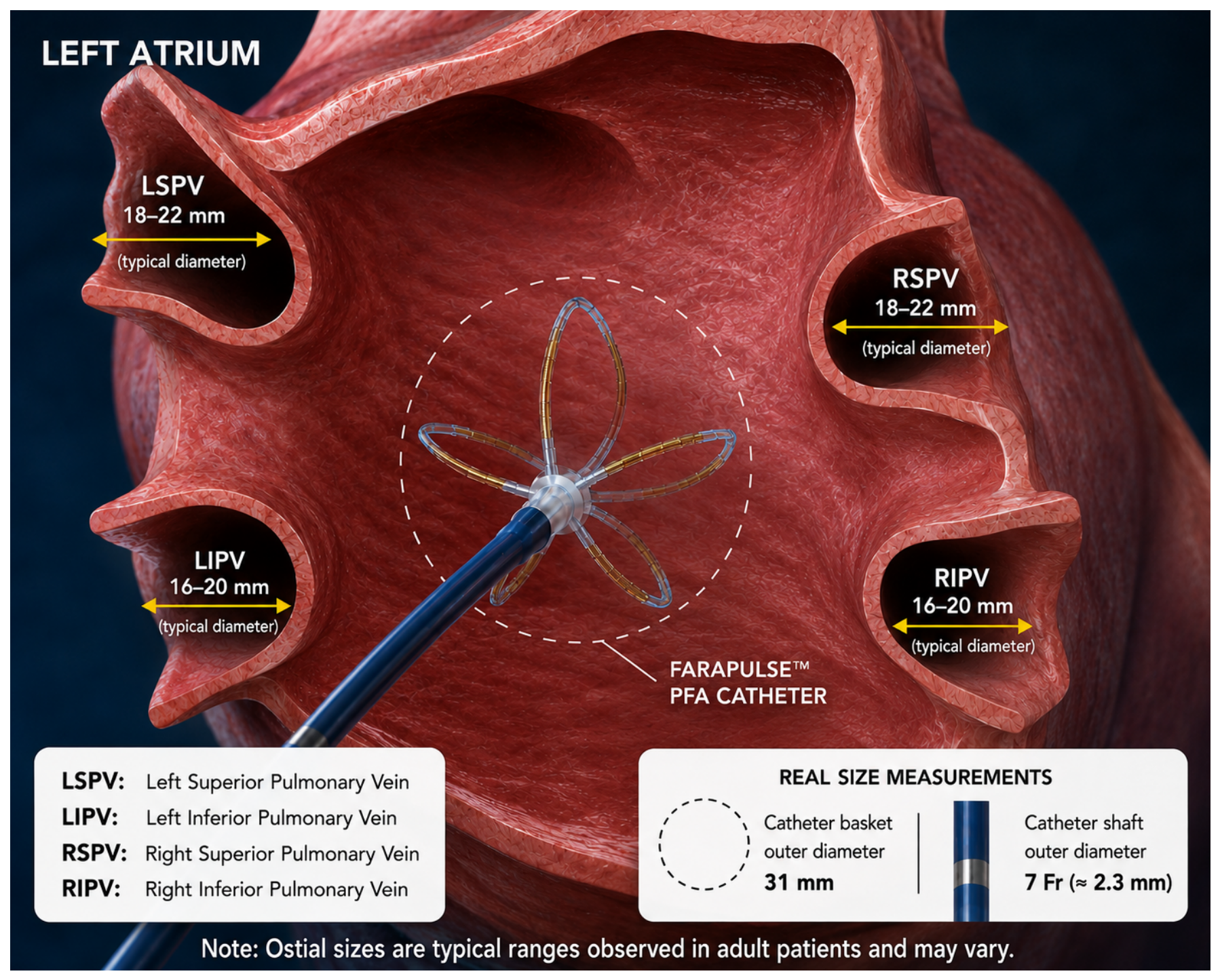
Figure 8 illustrates a realistic PFA setting, emphasizing the posterior chamber of the left atrium as well as the catheter within it. The scope of the present section is to provide an order-of-magnitude estimate of the volume of blood damaged during a PFA procedure. Therefore, to keep the level of complexity as low as possible, we model the chamber as a sphere of volume ${\mathfrak{V}}_{\mathrm{ch}}$, the radius of which is

$$R_{\mathrm{ch}}=\sqrt[3]{{\displaystyle \frac{3{\mathfrak{V}}_{\mathrm{ch}}}{4\pi }}}.$$

The volume ${\mathfrak{V}}_{\mathrm{ch}}$ fluctuates throughout the cardiac cycle, and reference values are sex-dependent. A reasonable estimate for ${\mathfrak{V}}_{\mathrm{ch}}$ is approximately 30 mL, so that $R_{\mathrm{ch}}\approx 19$ mm.

Figure 8. The FARAWAVE basket catheter can be modeled at first approximation as an array of approximately ten equivalent electric dipoles distributed over a quasi-spherical surface. The mean diameter of pulmonary veins is on the order 1.5–2.0 cm. The FARAWAVE basket is specifically designed to adapt to pulmonary vein ostia with diameters of approximately 15–30 mm, which are compatible with the typical dimensions of the pulmonary veins (schematic illustration generated with the assistance of OpenAI ChatGPT (GPT-5.5)).

We first estimate the volume of blood hemolyzed by a single pulse delivered by one pair of electrodes, i.e., a single dipole. The volume of damaged blood is

$${\mathfrak{V}}_{\mathrm{dam}}={\mathfrak{V}}_{\mathrm{ch}}{F}_{\mathrm{dam}}\left(R_{\mathrm{ch}}\right)$$

where, recalling (14),

$$F_{\mathrm{dam}}\left(R_{\mathrm{ch}}\right)={\displaystyle \frac{3}{2R_{\mathrm{ch}}^3}}{\int }_d^{R_{\mathrm{ch}}}H\left(\overline{E}\left(r\right)\right)r^{2}dr,$$

(17)

where the factor 1/2 reflects the fact that in a real PFA procedure blood occupies approximately only half of the region affected by the electric field, since each electrode of the device is in direct contact with the cardiac tissue.

We remark that the factor $0.5$ adopted in the present model should be interpreted as a nominal blood exposure coefficient rather than as a validated physiological constant. It represents an intermediate configuration between complete exposure of the electrodes to circulating blood and extensive catheter–tissue contact.

The introduction of such a correction factor is qualitatively supported by the study of Nies et al. [21], where the authors showed that hemolysis increases with the number of applications and is more pronounced when the catheter is fully exposed to blood than when it is in direct contact with tissue. After four applications, the measured free plasma hemoglobin concentration was $0.12\pm 0.03, \mathrm{g}/\mathrm{dL}$ in the no-contact configuration and $0.05\pm 0.03, \mathrm{g}/\mathrm{dL}$ in the contact configuration. These findings support the use of a blood exposure correction, although they do not provide a quantitative justification for selecting a $50\%$ reduction factor.

Recent clinical studies by Gianni et al. [19] and Kuraoka et al. [47] have also reported substantial differences among PFA platforms. These results indicate that voltage amplitude and application count cannot be considered as universal exposure descriptors, since they depend on catheter geometry, waveform, electrode configuration, and catheter–tissue contact. A quantitative assessment of the influence of all these factors would require detailed finite-element simulations based on platform- and patient-specific geometries, which is beyond the scope of the present work. The proposed framework is intended as a mathematically and physically consistent order-of-magnitude model aimed at identifying the principal scaling relationships among electric field intensity, device length scale, blood exposure, and number of deliveries rather than as a patient- or platform-specific treatment planning model.

We next consider the number $N_{\mathrm{elc}}$ of electrodes of the device (see Figure 8). If each $\left(-,+\right)$ electrode pair is regarded as a local dipole, the number of active dipoles is $N_{\mathrm{elc}}/2$. We note that the electric fields generated by adjacent electrode pairs partially overlap. However, to keep the model as simple as possible, we neglect this effect and approximate the total contribution as the sum of the individual contributions (if $l_i$ ($i=1,4$) are the four electrodes on a spline, we assume, again for simplicity, that the pair $(l_1,l_2)$ is independent by $(l_3,l_4)$). Therefore, the total fraction of damaged blood in one single pulse can be estimated as ${\displaystyle \frac{N_{\mathrm{elc}}}{2}}{F}_{\mathrm{dam}}\left(R_{\mathrm{ch}}\right)$. Consequently, the total volume of damaged blood in one single pulse is

$${\mathfrak{V}}_{\mathrm{dam},\mathrm{pulse}}={\displaystyle \frac{N_{\mathrm{elc}}}{2}}{F}_{\mathrm{dam}}\left(R_{\mathrm{ch}}\right){\mathfrak{V}}_{\mathrm{ch}},$$

(18)

with $F_{\mathrm{dam}}\left(R_{\mathrm{ch}}\right)$ given by (17).

To effectively apply (18) and obtain a reliable estimate of the total volume ${\mathfrak{V}}_{\mathrm{dam},\mathrm{tot}}$ of blood damaged during a complete PFA application, a few additional technical specifications are required.

For clarity, we distinguish the different levels of the PFA delivery hierarchy. An elementary biphasic pulse is a single voltage waveform with total duration $t_p$. A pulse train (or burst/packet) is a sequence of elementary biphasic pulses delivered during one activation of a given electrode pair (see Figure 2). A clinical application is a platform-specific sequence of electrode pair activations; for the system considered here, one application consists of five pulse trains. Catheter rotation is a mechanical repositioning performed between applications or groups of applications, and does not represent an additional electrical delivery; accordingly, ${\mathcal{N}}_{\mathrm{pulse}}$ denotes the total number of pulse trains rather than the number of elementary biphasic pulses.

We recall that ${\tau }_p$ is the time interval between the respective onsets of two consecutive pulse trains. We denote by ${\tau }_b$ the mean cardiac cycle duration. The model implicitly assumes uniform blood mixing; in reality, however, vortices within the left atrium and left atrial appendage, stagnation zones, and the complex geometry of the pulmonary veins may lead to incomplete blood renewal between consecutive pulses. Cardiac output is approximately $Q_{\mathrm{blood}}\approx 80$ mL/s, and the volume ${\mathfrak{V}}_{\mathrm{LA}}$ of the left atrium is ≈100–150 mL. Therefore, over a time interval of $0.5$ s, about 40 mL of blood flows through the atrium, which is a significant fraction of the whole atrium volume. This makes the assumption of “fresh” blood entering between successive pulses plausible. The ratio ${\tau }_p/{\tau }_b$ provides a simplified estimate of the fraction of pulse trains acting on freshly renewed and previously unexposed blood. Since ${\tau }_p<{\tau }_b$ in standard clinical practice, several consecutive trains act on substantially the same blood volume; for example, ${\tau }_p/{\tau }_b=0.5$ implies that approximately two trains are delivered within one cardiac cycle. Therefore, the effective number of trains acting on newly arrived blood is approximated as ${\mathcal{N}}_{\mathrm{pulse}}min\left(1,{\tau }_p/{\tau }_b\right).$ This expression is intended as an effective blood renewal correction within a simplified bounding model, and does not represent a substitute for a fully-resolved flow or residence time description.

We remark that electric pulses may also be delivered when the cardiac valves are open and the blood is moving. However, in order to obtain a conservative estimate of the volume of damaged blood, we consider the blood to be stationary within the atrial chamber.

Clearly, the previous reasoning provides only a rough estimate and has limited quantitative significance. Nevertheless, we believe that it yields a lower-bound estimate of the total volume of blood hemolyzed during a PFA session. Therefore, considering ${\tau }_p/{\tau }_b<1$, we estimate ${\mathfrak{V}}_{\mathrm{dam},\mathrm{tot}}$ as

$${\displaystyle \frac{{\tau }_p}{{\tau }_b}}{\mathcal{N}}_{\mathrm{pulse}}{\mathfrak{V}}_{\mathrm{dam},\mathrm{pulse}}\lesssim {\mathfrak{V}}_{\mathrm{dam},\mathrm{tot}}\lesssim {\mathcal{N}}_{\mathrm{pulse}}{\mathfrak{V}}_{\mathrm{dam},\mathrm{pulse}},$$

(19)

with ${\mathfrak{V}}_{\mathrm{dam},\mathrm{pulse}}$ given by (18). We remark that the present formulation is largely insensitive to the detailed waveform of the elementary pulse. Indeed, the specific pulse shape plays only a secondary role, affecting the predicted electric field through a numerical prefactor of order unity, provided that the peak voltage and pulse duration are comparable, since the model uses the peak electric field intensity as the relevant exposure measure. Consequently, triangular, rectangular, or sinusoidal waveforms lead to comparable order-of-magnitude estimates. The dominant source of uncertainty is instead the temporal spacing ${\tau }_p$ between consecutive elementary pulses relative to the cardiac cycle. For this reason, lower and upper bounds of the hemolyzed volume are obtained by considering different assumptions on blood renewal between pulses. Concerning ${\tau }_p$, in the what follows we refer to the caption of Figure 2.

The clinical protocol to isolate the four pulmonary veins generally requires several applications. To fix some numbers, we can reasonably assume four applications for each vein (the device is rotated four times each time), hence sixteen applications for the four veins. Each application consists in a train of five pulses, so we have a total ${\mathcal{N}}_{\mathrm{pulse}}\sim 80$ (note that these numbers are operator- and patient-dependent, and can change significantly).

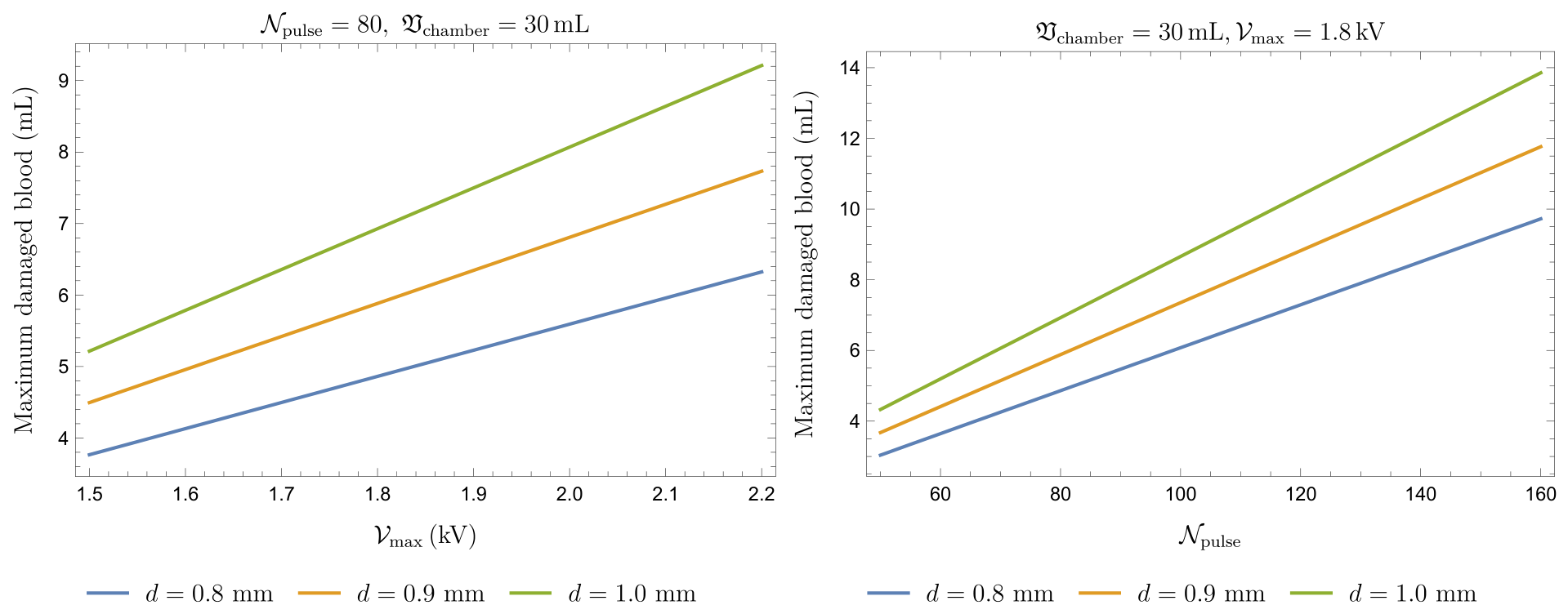
Figure 9 shows the maximum amount of damaged blood (in mL) under different choices of the operational parameters. More precisely, we observe the effects of varying the voltage for a given number of pulses (left panel) and varying the number of delivered pulses at a fixed voltage (right panel). In both cases, the volume of the chamber is fixed at 30 mL. The minimum amount of damaged blood is obtained by scaling the graphs in Figure 9 by a factor ${\tau }_b/{\tau }_p\approx 1/2$. Note that ${\mathfrak{V}}_{\mathrm{chamber}}$ is a physiological parameter that is fully patient-dependent and that d depends on the device manufacturer, whereas the applied voltage ${\mathcal{V}}_{\max }$ and the number of pulses ${\mathcal{N}}_{\mathrm{pulse}}$ dependent on the medical operator.

Figure 9. Maximum damaged blood (in mL) at the end of a complete clinical treatment while keeping some parameter fixed (see the upper plotlabel in each panel) and varying another specific one. Left Panel: Damage when varying ${\mathcal{V}}_{\max }\in (1.5,2.2)$ (kV). Right Panel: Damage when varying ${\mathcal{N}}_{\mathrm{pulse}}\in (50,160)$.

To compare ${\mathfrak{V}}_{\mathrm{dam},\mathrm{tot}}$ with clinical data, it is necessary to convert this value into the amount of fHb. Denoting by $v_{\mathrm{RBC}}$ the volume of a single RBC (typically $v_{\mathrm{RBC}}\approx 9\times {10}^{-11}{\mathrm{cm}}^3$) and by $\varphi$ the hematocrit (where normal values correspond to $\varphi \approx 0.45$), the number of RBCs in a given volume ${\mathfrak{V}}_{\mathrm{blood}}$ of blood is given by

$$N_{\mathrm{RBC}}\left({\mathfrak{V}}_{\mathrm{blood}}\right)\approx {\displaystyle \frac{\varphi }{v_{\mathrm{RBC}}}}{\mathfrak{V}}_{\mathrm{blood}}.$$

Assuming that each RBC contains approximately the same Hb mass $\gamma$ (typically $\gamma \approx 3\times {10}^{-11}$ g) and that all damaged RBCs are completely lysed, the concentration of Hb in plasma (i.e., fHb) with respect to the baseline level can be estimated as follows:

$$\Delta \mathrm{fHb}={\displaystyle \frac{\gamma }{(1-\varphi ){\mathfrak{V}}_{\mathrm{ref}}}}{\displaystyle \frac{\varphi }{v_{\mathrm{RBC}}}}{\mathfrak{V}}_{\mathrm{dam},\mathrm{tot}}$$

(20)

where ${\mathfrak{V}}_{\mathrm{dam},\mathrm{tot}}$ lies within the interval specified in (19) and ${\mathfrak{V}}_{\mathrm{ref}}$ is a reference volume (typically 5 L).

In Table 2, we report the estimated $\Delta$fHb (in g/L) when changing ${\mathcal{N}}_{\mathrm{pulse}}$ for ${\mathcal{V}}_{\max }=1.8$ (kV) and ${\mathcal{V}}_{\max }=2.2$ (kV), $d=0.9$ (mm), ${\mathfrak{V}}_{\mathrm{chamber}}=30$ (mL), $t_p=50$$\mathsf{\mu }$s, and $\varphi =0.45$. Table 3 shows the estimated $\Delta$fHb (in g/L) when changing ${\mathcal{V}}_{\max }$ (kV) for ${\mathcal{N}}_{\mathrm{pulse}}=120$, $d=0.9$ (mm), ${\mathfrak{V}}_{\mathrm{chamber}}=30$ (mL), $t_p=50$$\mathsf{\mu }$s, and $\varphi =0.45$. Finally, Table 4 shows the estimated $\Delta$fHb (in g/L) when changing ${\mathcal{V}}_{\max }$ for three values of $\varphi$, with ${\mathcal{N}}_{\mathrm{pulse}}=120$, $d=0.9$ (mm), ${\mathfrak{V}}_{\mathrm{chamber}}=30$ (mL), and $t_p=50$$\mathsf{\mu }$s.

Table 2. Estimated $\Delta$fHb (in g/L) for ${\mathcal{V}}_{\max }=1.8$ and 2.2 (kV) when changing ${\mathcal{N}}_{\mathrm{pulse}}$ with $d=0.9$ (mm), ${\mathfrak{V}}_{\mathrm{chamber}}=30$ mL, and $\varphi =0.45$.

${\mathcal{N}}_{\mathbf{pulse}}$	${\mathfrak{V}}_{\mathbf{dam},\mathbf{tot}}^{\left(\max \right)}$ (mL at 1.8 kV)	$\Delta$fHb	${\mathfrak{V}}_{\mathbf{dam},\mathbf{tot}}^{\left(\max \right)}$ (mL at 2.2 kV)	$\Delta$fHb (g/L)
30	2.21	0.12	2.9	0.16
40	2.94	0.16	3.87	0.21
50	3.68	0.20	4.83	0.26
60	4.41	0.24	5.8	0.32
70	5.15	0.28	6.77	0.37
80	5.88	0.32	7.73	0.42
90	6.62	0.36	8.7	0.47
100	7.35	0.40	9.67	0.53
110	8.09	0.44	10.63	0.58
120	8.82	0.48	11.6	0.63

Table 3. Estimated $\Delta$fHb (in g/L) when changing ${\mathcal{V}}_{\max }$ (kV) for ${\mathcal{N}}_{\mathrm{pulse}}=80$, $d=0.9$ (mm), ${\mathfrak{V}}_{\mathrm{chamber}}=30$ (mL), and $\varphi =0.45$.

${\mathcal{V}}_{\mathbf{max}}$	${\mathfrak{V}}_{\mathbf{dam},\mathbf{tot}}^{\left(\max \right)}$ (mL)	$\Delta$fHb (g/L)
1.5	4.5	0.25
1.6	4.96	0.27
1.7	5.42	0.3
1.8	5.88	0.32
1.9	6.35	0.35
2.	6.81	0.37
2.1	7.27	0.4
2.2	7.73	0.42

Table 4. Estimated $\Delta$fHb (in g/L) when changing ${\mathcal{V}}_{\max }$ for three values of $\varphi$, with ${\mathcal{N}}_{\mathrm{pulse}}=80$, $d=0.9$ (mm), ${\mathfrak{V}}_{\mathrm{chamber}}=30$ (mL), $t_p=50$$\mathsf{\mu }$s.

${\mathcal{V}}_{\mathbf{max}}$	${\mathfrak{V}}_{\mathbf{dam},\mathbf{tot}}$ (mL)	$\Delta {\mathbf{fHb}}_{\mathit{\varphi }=0.4}$	$\Delta {\mathbf{fHb}}_{\mathit{\varphi }=0.45}$	$\Delta {\mathbf{fHb}}_{\mathit{\varphi }=0.5}$
1.5	4.5	0.20	0.25	0.30
1.6	4.96	0.22	0.27	0.33
1.7	5.42	0.24	0.30	0.36
1.8	5.88	0.26	0.32	0.39
1.9	6.35	0.28	0.35	0.42
2.	6.81	0.3	0.37	0.45
2.1	7.27	0.32	0.40	0.48
2.2	7.73	0.34	0.42	0.52

So far as we know, the measured values of $\Delta$fHb in the framework of a standard PFA complete treatment range from 0.1 to 1 g/L (in procedures with a large number of deliveries; for example, see Figure 3 in [18]). From this point of view, the predictions of the mathematical model appear to be close to clinical data.

However, it is important to remark that the estimate in (20) is largely approximate. There are several reasons for this: first, the geometric simplifications introduced to make the model tractable inevitably reduce its accuracy; second, the assumption that each pulse interacts with a completely new blood volume is likely unrealistic, as incomplete mixing, recirculation, and stagnation zones may lead to repeated exposure of the same blood; third, in clinical PFA some erythrocytes may undergo only reversible or sublethal membrane damage; finally, the non-uniform electric field distribution and several physiological processes, including systemic dilution, haptoglobin binding, renal and macrophage-mediated clearance, hydration, redistribution, baseline free hemoglobin, and sampling time, are not included in the present model. These mechanisms may influence the relationship between the released hemoglobin mass and the clinically measured free hemoglobin concentration. They are mentioned here solely as limitations of the current formulation, and are not invoked as post hoc explanations for any discrepancies between model predictions and experimental data.

3. Comparison with Clinical and Experimental Data

There are relatively few papers aimed at providing quantitative estimates of blood damage induced by high-intensity electric fields. Besides the seminal works by Zimmermann [15] and Kinosita and Tsong [40], we note the studies by Montoya et al. [46], Popa et al. [18], Fiserova et al. [26], Kuraoka et al. [47], and Gianni et al. [19].

The study by Montoya et al. [46] is primarily based on PFA computational modeling. In that work, a single 2 kV pulse was applied to a blood sample, though the exposed blood volume was not specified by the authors. The estimated hemolyzed blood volume was approximately 38 $\mathsf{\mu }$L (for the case of electrodes not in direct contact with endocardial tissue and exposed to the blood pool). Since our model estimates the amount of hemolyzed blood as a fraction of the total blood volume, it cannot be directly compared with the data in [46]. However, starting from (9), we can estimate the volume in which the electric field exceeds the threshold $E_{50}$, which can be taken as the hemolysis threshold (we note, however, that Montoya et al. did not specify the value of $E_{50}$). Hence, by solving $\overline{E}\left(\xi \right)=E_{50}$, we determine ${\xi }_{\mathrm{hem}}$, i.e.,

$${\xi }_{\mathrm{hem}}=\sqrt[3]{{\displaystyle \frac{0.31{\mathcal{V}}_{\max }}{d{E}_{50}}}},$$

and consequently the radius of the sphere within which almost 50% of the blood is hemolyzed, denoted by $R_{\mathrm{hem}}={\xi }_{\mathrm{hem}}d$. Therefore, the hemolyzed blood volume in a single pulse, ${\mathfrak{V}}_{\mathrm{hem}}$, is

$${\mathfrak{V}}_{\mathrm{hem}}={\displaystyle \frac{4}{3}}\pi d^3\left({\xi }_{\mathrm{hem}}^3-1\right),$$

which we compare with the 38 $\mathsf{\mu }$L reported by Montoya et al. For $E_{50}=1.85$ (kV/cm), our model underestimates the values of Montoya et al. [46] by a factor of 4–5 (see Table 5). However, it should be noted that Montoya et al. provided no indication of the relationship used to correlate the electric field with the percentage of hemolyzed blood. A lower effective hemolysis threshold would substantially increase the predicted hemolyzed volume. Therefore, the missing exposure–response relationship in [46] represents an important source of uncertainty, as clearly emphasized by Table 5.

Table 5. Comparison with the computational estimate of Montoya et al. [46] by varying ${\mathcal{V}}_{\max }$ and $E_{50}$ with $d=0.9$ mm for a single pulse delivery.

	${\mathit{E}}_{50}=1.85$ (kV/cm)	${\mathit{E}}_{50}=1.45$ (kV/cm)	${\mathit{E}}_{50}=1.05$ (kV/cm)
${\mathcal{V}}_{\mathbf{max}}$	${\mathfrak{V}}_{\mathbf{hem}}\mathbf{(}\mathbf{\mu }\mathrm{L}\mathbf{)}$	${\mathfrak{V}}_{\mathbf{hem}}\mathbf{(}\mathbf{\mu }\mathbf{L}\mathbf{)}$	${\mathfrak{V}}_{\mathbf{hem}}\mathbf{(}\mathbf{\mu }\mathbf{L}\mathbf{)}$
1.8	7.18	10.03	15.88
1.9	7.75	10.73	15.93
2.0	8.32	11.45	17.98
2.1	8.89	12.18	19.03
2.2	9.45	12.9	20.09

The clinical study by Popa et al. [18] investigated hemolysis following PFA using a FARAWAVE catheter (Boston Scientific Corporation, Marlborough, MA, USA) operated at 2 kV. The authors reported a mean fHb concentration of $0.6\pm 0.3$ g/L immediately after the procedure, with an average of $61.6\pm 27.4$ PFA deliveries. Furthermore, a significant positive correlation was observed between fHb levels and the number of PFA applications, indicating a dose-dependent increase in hemolysis. Their findings provide a useful benchmark for the proposed model. Our model predicts 0.4 g/L of fHb after 70 pulses (see Table 2), which is comparable to the values reported by Popa et al. Even at the extreme values of the number of deliveries reported in [18], our predictions remain within the same order of magnitude. Moreover, considering the experimentally observed correlation between hemolysis and the number of PFA deliveries, any discrepancy may be partly explained by physiological mechanisms such as dilution, recirculation, haptoglobin binding, and hemoglobin clearance, which are not explicitly included in the current formulation. In conclusion, comparison with the clinical data of Popa et al. suggests that our model provides a realistic order-of-magnitude estimate of PFA-induced hemolysis and supports its use as a first quantitative framework for predicting free hemoglobin release during PFA procedures.

Unlike the computational study of Montoya et al., the work of Fiserova et al. [26] is largely based on experimental measurements and provides an empirical relationship between free hemoglobin concentration and electric field intensity. Their data show negligible hemolysis at 0.75 kV/cm, whereas free hemoglobin increases to approximately 2.2 g/L at 1 kV/cm and 5.7 g/L at 1.5 kV/cm. However, their experimental protocol differs substantially from clinical PFA practice, employing 20 bursts of 216 bipolar pulses (2 $\mathsf{\mu }$s duration, 5 $\mathsf{\mu }$s inter-pulse interval) repeated 20 times, for a total of 4320 pulses. Owing to these significant differences in pulse structure and total delivered dose, a direct quantitative comparison with the present model is difficult.

As far as the study by Kuraoka et al. is concerned, the present model cannot be directly validated against the data reported in [47] because it estimates the cumulative free hemoglobin concentration from the hemolyzed blood volume generated by each individual PFA pulse, whereas the clinical study in [47] reports only the final post-procedural biomarker levels. Nevertheless, the predicted cumulative fHb concentrations are in satisfactory agreement with the clinical observations in terms of order of magnitude.

A similar consideration applies to the study by Gianni et al. [19]. The present model is not intended to reproduce patient-specific clinical measurements; rather, it provides a physics-based estimate of the cumulative free hemoglobin released during the procedure. Consequently, a direct quantitative comparison is not feasible. Nevertheless, the predicted post-procedural fHb concentrations are consistent with the values reported in the clinical study in terms of order of magnitude.

Overall, the present model estimates hemolysis from the spatial distribution of the electric field and the resulting hemolyzed blood volume generated by each pulse, whereas the available clinical studies report only cumulative hemolysis biomarkers measured at the end of the procedure. Therefore, the comparison should be regarded as qualitative rather than quantitative, with agreement being assessed primarily in terms of the predicted order of magnitude of the final fHb concentration.

4. Conclusions

Pulsed Field Ablation (PFA) has been increasingly adopted as a non-thermal strategy (although some caution remains warranted) for the treatment of cardiac arrhythmias. Although its primary mechanism relies on the selective irreversible electroporation of cardiomyocytes, exposure of circulating blood to intense electric fields may induce red blood cell injury and hemolysis. Understanding the magnitude of this effect is important both for the interpretation of clinical biomarkers and for the optimization of future PFA protocols.

In this work, we develop a simplified mathematical–physical model aimed at estimating the amount of hemolyzed blood and the corresponding release of free hemoglobin during PFA procedures. The model combines a dipolar representation of the electric field generated by the catheter with experimentally derived hemolysis–response relationships obtained from classical electroporation studies. Particular attention is devoted to the distinction between membrane poration and actual hemoglobin release, which motivated the choice of Kinosita and Tsong’s experimental data.

The analysis indicates that clinically relevant hemolysis is expected only within a limited region surrounding the electrodes, where the electric field exceeds a threshold of a few kV/cm. Model predictions suggest free hemoglobin concentrations generally ranging from approximately 0.1 to 0.6 g/L for typical PFA operating conditions, in reasonable agreement with currently available clinical observations. For example, the predicted dependence of hemolysis on pulse number and delivered electrical dose is consistent with the trends reported in recent clinical studies.

The proposed framework is intentionally simplified and should be regarded primarily as an order-of-magnitude model. Several potentially important mechanisms are not included, including detailed catheter geometry, blood flow dynamics, pulse-to-pulse resealing, heterogeneous field distributions, erythrocyte deformation, and physiological clearance of free hemoglobin; consequently, the quantitative predictions should be interpreted with caution.

Despite these limitations, the proposed framework provides a mechanistic link between electric field exposure and free hemoglobin release, offering a qualitative tool for estimating the order of magnitude of the volume of blood damaged during PFA, though not a precise quantitative prediction. Future developments should incorporate realistic catheter geometries, patient-specific atrial anatomies, and dedicated experimental measurements of hemoglobin release under PFA-like conditions. Such improvements could contribute to the definition of safer treatment protocols and to a deeper understanding of the biological effects of cardiac electroporation.

We remark that generative AI has been used in our study only for the preparation of some schematic illustrations (clearly declared in their specific captions), and never contributed to the scientific analysis. However, we think that physics-based models and AI should not be regarded as competing approaches. The present equations offer interpretability, mechanistic constraints, and the possibility of extrapolating from established biophysical principles. Conversely, machine learning methods could help to estimate uncertain model parameters, construct computationally efficient surrogate models of complex electric field distributions, integrate patient-specific anatomy and procedural data, and identify nonlinear interactions that are not captured by the present simplified geometry. Hybrid physics-informed or mechanistically constrained AI models may provide a useful future direction, particularly after sufficiently large experimental and clinical datasets become available (see, e.g., [48]).

Appendix A.1

The content of this section relies mostly on the classical theory of electromagnetism [43]. Nevertheless, it has been added to help the reader familiar with PFA but not equally so with PDE to understand the use of Formula (9) in Section 2.1.

Appendix A.2. Geometry of the Problem

We consider spherical coordinates

$$x=r\sin \theta \cos \varphi ,y=r\sin \theta \sin \varphi ,z=r\cos \theta$$

with $r>0$, $0<\theta <\pi$, $-\pi <\varphi <\pi$, and consider two identical metallic spheres of radius $a=d/4$ placed symmetrically with respect to the origin and with their centers on the x-axis. The centers of the two spheres are respectively

$${\mathit{r}}_1=-\left({\displaystyle \frac{d}{4}}+{\displaystyle \frac{d}{2}}\right){\mathit{e}}_x=-{\displaystyle \frac{3d}{4}}{\mathit{e}}_x,{\mathit{r}}_2=+\left({\displaystyle \frac{d}{4}}+{\displaystyle \frac{d}{2}}\right){\mathit{e}}_x=+{\displaystyle \frac{3d}{4}}{\mathit{e}}_x.$$

Therefore, the distance between the two centers is $3d/2$, while the distance between the two closest points of the two spheres is d. The surface of the left sphere is kept at potential $+\mathcal{V}/2$, whereas the surface of the right one is kept at potential $-\mathcal{V}/2$. Therefore, the voltage difference between the two metallic spheres is $\mathcal{V}$. Since the potentials of the two conductors are prescribed, the electric field in the quasi-static approximation is obtained from the electrostatic potential as $\mathit{E}=-\nabla \Phi .$ For a homogeneous medium, the function $\Phi$ satisfies Laplace’s equation outside the two spheres: ${\nabla }^2\Phi =0.$

Appendix A.3. Bispherical Coordinates

The natural coordinates for this problem are bispherical coordinates with the axis along the Cartesian x-axis (see Figure A1).

Figure A1. Geometrical representation of bispherical coordinate lines in the plane (schematic illustration generated with the assistance of OpenAI ChatGPT (GPT-5.5)).

Figure A1. Geometrical representation of bispherical coordinate lines in the plane (schematic illustration generated with the assistance of OpenAI ChatGPT (GPT-5.5)).

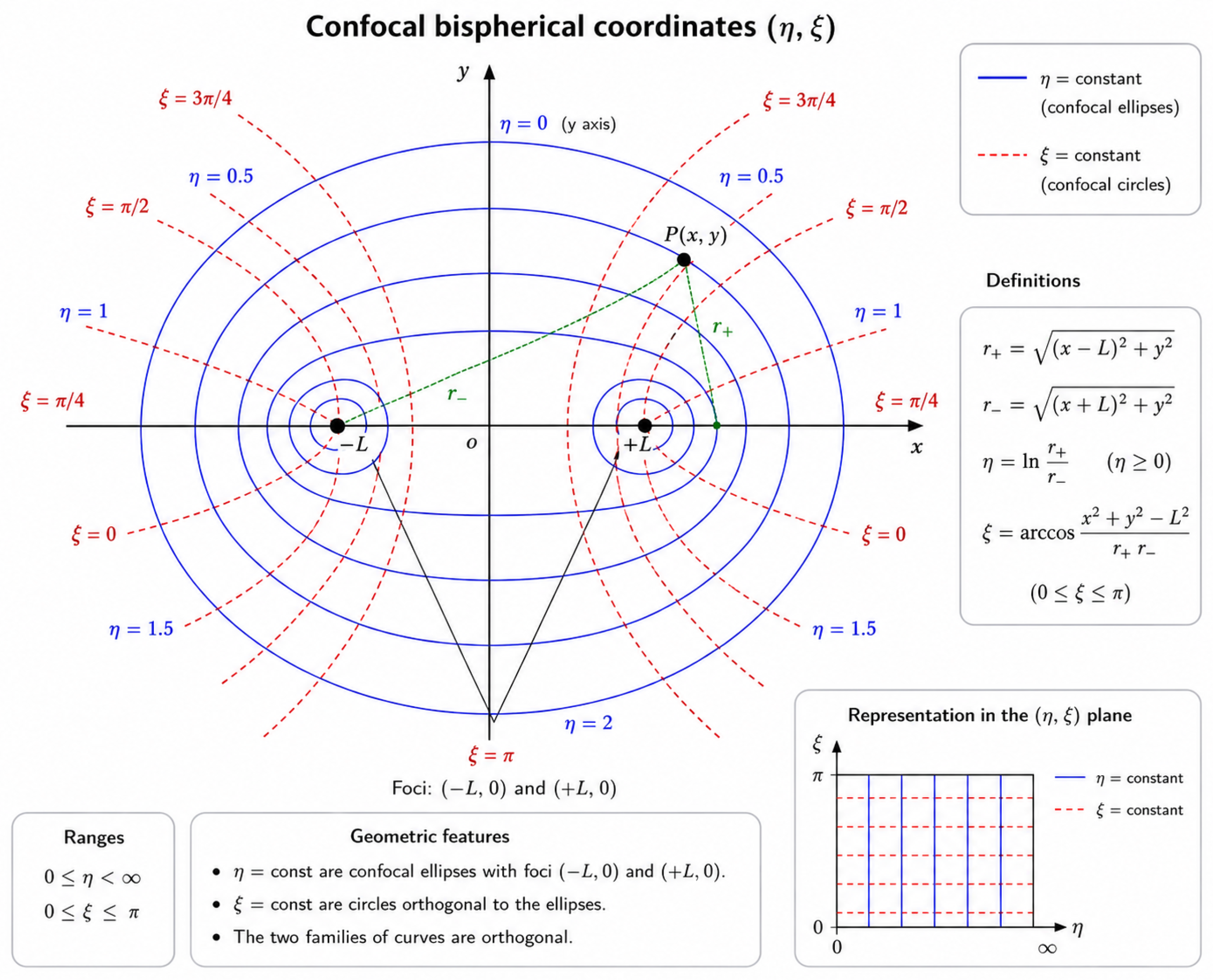
Let $h=3d/4$, placing the centers of the two spheres are at $x_c=\pm h$. Set $a=d/4$ (radius of the spheres) and define $\mathsf{\ell }=\sqrt{h^2-a^2}$. Then, $\mathsf{\ell }=d/\sqrt{2}$. The bispherical coordinates $(\xi ,\eta )$ are defined as

$$x={\displaystyle \frac{\mathsf{\ell }sinh\eta }{\cosh \eta -\cos \xi }}$$

and

$$\rho =\sqrt{y^2+z^2}={\displaystyle \frac{\mathsf{\ell }\sin \xi }{\cosh \eta -\cos \xi }}.$$

We also define $\cosh {\eta }_0=h/a.$ Then, in bispherical coordinates, the two spherical surfaces are respectively represented by ${\eta }_{\mp }=\pm {\eta }_0$. Their geometrical parameters are $a=\mathsf{\ell }/sinh{\eta }_0$ and $x_c=\pm \mathsf{\ell }coth{\eta }_0$, respectively.

Appendix A.4. Electrostatic Potential

The electrostatic potential outside the two spheres is [43]

$$\Phi (\eta ,\xi )=\sqrt{D}{\displaystyle \sum _{n=0}^{\infty }}{A}_{n}sinh\left[\left(n+{\displaystyle \frac{1}{2}}\right)\eta \right]P_n\left(\cos \xi \right),$$

where $P_n$ are Legendre polynomials and $D=\cosh \eta -\cos \xi$. Let us define $k_n=n+1/2$; then,

$$A_n=-{\displaystyle \frac{\mathcal{V}}{\sqrt{2}}}{\displaystyle \frac{exp(-k_n{\eta }_0)}{sinh\left(k_n{\eta }_0\right)}}.$$

With this choice, $\Phi (-{\eta }_0,\xi )=+\mathcal{V}/2$ and $\Phi (+{\eta }_0,\xi )=-\mathcal{V}/2$; also, $\Phi \to 0$ as $r\to \infty .$

Appendix A.5. Electric Field

The electric field $\mathit{E}=-\nabla \Phi$ in bispherical coordinates is given by

$$\mathit{E}=-{\displaystyle \frac{D}{\mathsf{\ell }}}\left[{\displaystyle \frac{\partial \Phi }{\partial \eta }}{\mathit{e}}_{\eta }+{\displaystyle \frac{\partial \Phi }{\partial \xi }}{\mathit{e}}_{\xi }\right].$$

The two derivatives of the potential are

$$\begin{array}{cc}\hfill {\displaystyle \frac{\partial \Phi }{\partial \eta }}& ={\displaystyle \frac{sinh\eta }{2\sqrt{D}}}{\displaystyle \sum _{n=0}^{\infty }}{A}_{n}sinh\left(k_n\eta \right)P_n\left(\cos \xi \right)+\sqrt{D}{\displaystyle \sum _{n=0}^{\infty }}{A}_n{k}_n\cosh \left(k_n\eta \right)P_n\left(\cos \xi \right)\hfill \end{array}$$

and

$$\begin{array}{cc}\hfill {\displaystyle \frac{\partial \Phi }{\partial \xi }}& ={\displaystyle \frac{\sin \xi }{2\sqrt{D}}}{\displaystyle \sum _{n=0}^{\infty }}{A}_{n}sinh\left(k_n\eta \right)P_n\left(\cos \xi \right)-\sqrt{D}\sin \xi {\displaystyle \sum _{n=0}^{\infty }}{A}_{n}sinh\left(k_n\eta \right)P_n^{\prime }\left(\cos \xi \right).\hfill \end{array}$$

Therefore, the exact electric field outside the two metallic spheres is

$$\mathit{E}=-{\displaystyle \frac{D}{\mathsf{\ell }}}\left[{\displaystyle \frac{\partial \Phi }{\partial \eta }}{\mathit{e}}_{\eta }+{\displaystyle \frac{\partial \Phi }{\partial \xi }}{\mathit{e}}_{\xi }\right].$$

The magnitude $E=\left|\mathit{E}\right|$ of the electric field is obtained directly in bispherical coordinates:

$$E={\displaystyle \frac{D}{\mathsf{\ell }}}{\left[{\left({\displaystyle \frac{\partial \Phi }{\partial \eta }}\right)}^2+{\left({\displaystyle \frac{\partial \Phi }{\partial \xi }}\right)}^2\right]}^{1/2}.$$

Appendix A.6. Angular Average of the Field Magnitude

We want to find the average of E over the full solid angle at fixed r:

$$\overline{E}\left(r\right)={\displaystyle \frac{1}{4\pi }}{\int }_{4\pi }\left|\mathit{E}(r,\theta ,\varphi )\right|d\Omega .$$

Because the system is axially symmetric around the x-axis, the magnitude of the field depends on the angles only through $u=\sin \theta \cos \varphi .$ Therefore,

$$\overline{E}\left(r\right)={\displaystyle \frac{1}{2}}{\int }_{-1}^1\left|\mathit{E}(r,u)\right|du.$$

For each value of r and u, define

$$\Gamma (r,u)={\left[{\left(r^2+{\mathsf{\ell }}^2\right)}^2-4{\mathsf{\ell }}^2{r}^2{u}^2\right]}^{1/2}.$$

Then,

$$\cosh \eta (r,u)={\displaystyle \frac{r^2+{\mathsf{\ell }}^2}{\Gamma (r,u)}},sinh\eta (r,u)={\displaystyle \frac{2\mathsf{\ell }ru}{\Gamma (r,u)}},\cos \xi (r,u)={\displaystyle \frac{r^2-{\mathsf{\ell }}^2}{\Gamma (r,u)}}.$$

Moreover,

$$D(r,u)=\cosh \eta (r,u)-\cos \xi (r,u).$$

Hence,

$$\begin{array}{cc}\hfill \overline{E}\left(r\right)& ={\displaystyle \frac{1}{2}}{\int }_{-1}^1{\displaystyle \frac{D(r,u)}{\mathsf{\ell }}}{\left[{\left({\displaystyle \frac{\partial \Phi }{\partial \eta }}\right)}^2+{\left({\displaystyle \frac{\partial \Phi }{\partial \xi }}\right)}^2\right]}^{1/2}du.\hfill \end{array}$$

In this formula, the derivatives are evaluated at $\eta =\eta (r,u),\xi =\xi (r,u).$ This is the exact angular average of the field magnitude for $r>d$.

Appendix A.7. Power-Series Expansion in d/r

Let us examine the region $r>d$, more specifically, the far-field regime ${\displaystyle \frac{d}{r}}\ll 1.$ Since the two metallic spheres are kept at symmetric potentials $+\mathcal{V}/2$ and $-\mathcal{V}/2,$ the total charge of the system is zero, so the monopole term is absent. The leading far-field term is dipolar. Consequently, $\overline{E}\left(r\right)$ scales as $1/r^3.$ For the special geometry $a=d/4,$ the angular average has the expansion

$$\overline{E}\left(r\right)={\displaystyle \frac{\left|\mathcal{V}\right|}{d}}\left[C_1{\left({\displaystyle \frac{d}{r}}\right)}^3+C_3{\left({\displaystyle \frac{d}{r}}\right)}^5+O\left({\displaystyle \frac{d^7}{r^7}}\right)\right].$$

When rounded to two significant digits, the numerical coefficients are

$$C_1\simeq 0.31,C_3\simeq -0.040.$$

Factoring out the leading term gives

$$\overline{E}\left(r\right)\simeq 0.31{\displaystyle \frac{\left|\mathcal{V}\right|d^2}{r^3}}\left[1-0.13{\left({\displaystyle \frac{d}{r}}\right)}^2\right].$$

Thus, the leading approximation is

$$\overline{E}\left(r\right)\simeq 0.31{\displaystyle \frac{\left|\mathcal{V}\right|d^2}{r^3}}.$$

If only the first term of the expansion is kept, the neglected relative correction is approximately

$$\Delta \overline{E}\left(r\right)\simeq 0.13{\left({\displaystyle \frac{d}{r}}\right)}^2.$$

Since we are considering $r>d,$ the maximum estimated relative error is obtained near $r=d$, that is, ${\Delta }_{\max }\simeq 0.13.$ For example, for $r=2d$ we have $\Delta \simeq 3.3\%$; similarly, for $r=3d$ we have $\Delta \simeq 1.4\%$.

References

- Verma, A.; Asivatham, S.J.; Deneke, T.; Castellvi, Q.; Neal, R.E. Primer on pulsed electrical field ablation: Understanding the benefits and limitations. Circ. Arrhythmia Electrophysiol. 2021, 14, e010086. [Google Scholar]
- Chun, K.-R.J.; Miklavčič, D.; Vlachos, K.; Bordignon, S.; Scherr, D.; Jais, P.; Schmidt, B. State-of-the-art pulsed field ablation for cardiac arrhythmias: Ongoing evolution and future perspective. Europace 2024, 26, euae134. [Google Scholar] [CrossRef] [Scilit] [PubMed]
- Weaver, J.C. Electroporation theory: Concepts and mechanisms. Methods Mol. Biol. 1995, 55, 3–28. [Google Scholar] [CrossRef] [Scilit] [PubMed]
- Weaver, J.C.; Chizmadzhev, Y.A. Theory of electroporation: A review. Bioelectrochem. Bioenerg. 1996, 41, 135–160. [Google Scholar] [CrossRef] [Scilit]
- Weaver, J.C. Electroporation of cells and tissues. IEEE Trans. Plasma Sci. 2002, 28, 24–33. [Google Scholar]
- Kotnik, T.; Kramar, P.; Pucihar, G.; Miklavcic, D.; Tarek, M. Cell membrane electroporation-part 1: The phenomenon. IEEE Electr. Insul. Mag. 2012, 28, 14–23. [Google Scholar] [CrossRef] [Scilit]
- Grimaldi, M.; Di Monaco, A.; Gomez, T.; Berman, D.; Datta, K.; Sharma, T.; Govari, A.; Altmann, A.; Di Biase, L. Time course of irreversible electroporation lesion development through short-and long-term follow-up in pulsed-field ablation–treated hearts. Circ. Arrhythmia Electrophysiol. 2022, 15, e010661. [Google Scholar] [CrossRef] [Scilit] [PubMed]
- Kirstein, B.; Heeger, C.-H.; Vogler, J.; Eitel, C.; Feher, M.; Phan, H.-L.; Mushfiq, I.; Traub, A.; Hatahet, S.; Samara, O.; et al. Impact of pulsed field ablation on intraluminal esophageal temperature. J. Cardiovasc. Electrophysiol. 2024, 35, 78–85. [Google Scholar] [CrossRef] [Scilit] [PubMed]
- Farina, A.; Fasano, A.; Grimaldi, M.; Rosso, F. Heat delivery accompanying pulsed field ablation. J. Theor. Biol. 2025, 610, 112145. [Google Scholar] [CrossRef] [Scilit] [PubMed]
- Mercado-Montoya, M.; Gomez-Bustamante, T.; Mickelsen, S.R.; Kulstad, E.; González-Suárez, A.; Overzet, L.J. Thermal side effects during pulsed field ablation: An analysis using computer modelling. Europace 2025, 27, euaf035. [Google Scholar] [CrossRef] [Scilit] [PubMed]
- Nies, M.; Koruth, J.S.; Mlček, M.; Petru, J.; Tibenská, V.C.; Watanabe, K.; Královec, Š.; Hala, P.; Tejkl, L.; Neuzil, P.; et al. Is the esophagus spared during pulsed field ablation? early histopathology and in vivo esophageal retraction. Heart Rhythm 2026, 23, 788–799. [Google Scholar] [CrossRef] [Scilit] [PubMed]
- Di Monaco, A.; Fasano, A.; Farina, A.; Rosso, F.; Grimaldi, M. Is the esophagus spared during pulsed field ablation? Pacing Clin. Electrophysiol. 2026, 49, 665–668. [Google Scholar] [CrossRef] [Scilit] [PubMed]
- Kocharian, A.A.; Murthy, M.K.; Patel, A.; Venkataraman, R.; Mathuria, N.S.; Lador, A.; Fahed, J.; Valderrábano, M. Luminal esophageal temperature rises with pulsed field ablation. Clin. Electrophysiol. 2025, 11, 1033–1035. [Google Scholar] [CrossRef] [Scilit] [PubMed]
- Lei, D.; Xiang, B.; Qi, Y.; Liu, Y.; Zhang, K.; Jiang, Z.; Yu, F.; Zhang, H.; Tang, M. Hemolysis and kidney injury after catheter ablation for atrial fibrillation: Microsecond vs nanosecond pulsed field ablation. Heart Rhythm 2026, 23, e1897–e1906. [Google Scholar] [CrossRef] [Scilit] [PubMed]
- Zimmermann, U.; Pilwat, G.; Riemann, F. Dielectric breakdown of cell membranes. Biophys. J. 1974, 14, 881–899. [Google Scholar] [CrossRef] [Scilit] [PubMed]
- Kinosita, K., Jr.; Tsong, T.T. Hemolysis of human erythrocytes by transient electric field. Proc. Natl. Acad. Sci. USA 1977, 74, 1923–1927. [Google Scholar] [CrossRef] [Scilit] [PubMed]
- Kinosita, K.; Ashikawa, I.; Saita, N.; Yoshimura, H.; Itoh, H.; Nagayama, K.; Ikegami, A. Electroporation of cell membrane visualized under a pulsed-laser fluorescence microscope. Biophys. J. 1988, 53, 1015–1019. [Google Scholar] [CrossRef] [Scilit] [PubMed]
- Popa, M.A.; Venier, S.; Menè, R.; Della Rocca, D.G.; Sacher, F.; Derval, N.; Hocini, M.; Dulucq, S.; Caluori, G.; Combes, S.; et al. Characterization and clinical significance of hemolysis after pulsed field ablation for atrial fibrillation: Results of a multicenter analysis. Circ. Arrhythmia Electrophysiol. 2024, 17, e012732. [Google Scholar] [CrossRef] [Scilit] [PubMed]
- Gianni, C.; Al-Ahmad, A.; Elchouemi, M.; Mirco La Fazia, V.; Mohanty, S.; Allison, J.D.; Bassiouny, M.A.; Bode, W.D.; Burkhardt, J.D.; Coffeen, P.C.; et al. Pulsed field ablation–related hemolysis: Comparison between technologies. Circ. Arrhythmia Electrophysiol. 2026, 18, e014021. [Google Scholar] [CrossRef] [Scilit] [PubMed]
- Venier, S.; Vaxelaire, N.; Jacon, P.; Carabelli, A.; Desbiolles, A.; Garban, F.; Defaye, P. Severe acute kidney injury related to haemolysis after pulsed field ablation for atrial fibrillation. Europace 2024, 26, euad371. [Google Scholar] [CrossRef] [Scilit] [PubMed]
- Nies, M.; Koruth, J.S.; Mlček, M.; Watanabe, K.; Tibenská, V.C.; Královec, Š.; Tejkl, L.; Neuzil, P.; Reddy, V.Y. Hemolysis after pulsed field ablation: Impact of lesion number and catheter-tissue contact. Circ. Arrhythmia Electrophysiol. 2024, 17, e012765. [Google Scholar] [CrossRef] [Scilit] [PubMed]
- Saulis, G.; Venslauskas, M.S.; Naktinis, J. Kinetics of pore resealing in cell membranes after electroporation. J. Electroanal. Chem. Interfacial Electrochem. 1991, 321, 1–13. [Google Scholar] [CrossRef] [Scilit]
- Giersiepen, M.; Wurzinger, L.J.; Opitz, R.; Reul, H. Estimation of shear stress-related blood damage in heart valve prostheses-in vitro comparison of 25 aortic valves. Int. J. Artif. Organs 1990, 13, 300–306. [Google Scholar] [CrossRef] [Scilit]
- Bruss, J.; Kueffer, T.; Tanner, H.; Noti, F.; Haeberlin, A.; Thalmann, G.; Asenov Kozhuharov, N.; Kovacs, B.; Spahiu, V.; Herrera Siklody, C.; et al. Hemolysis induced by pulsed-field ablation of atrial arrhythmias: A comparative analysis of current systems. J. Cardiovasc. Electrophysiol. 2025, 36, 2498–2506. [Google Scholar] [CrossRef] [Scilit] [PubMed]
- Cersosimo, A.; Pierucci, N.; Mariani, M.V.; Matteucci, A.; Parato, A.G.; La Fazia, V.M.; Natale, A. Hemolysis in pulsed field ablation for atrial fibrillation: A narrative review. Rev. Cardiovasc. Med. 2026, 27, 46485. [Google Scholar] [CrossRef] [Scilit] [PubMed]
- Fiserova, I.; Fiser, O.; Novak, M.; Trnka, J.; Gibalova, A.; Kvapil, D.; Bacova, B.; Hozman, M.; Herman, D.; Benesova, K.; et al. Significant hemolysis is present during irreversible electroporation of cardiomyocytes in vitro. Heart Rhythm 2025, 22, 466–474. [Google Scholar] [CrossRef] [Scilit] [PubMed]
- Borsi, I.; Farina, A.; Fasano, A.; Rajagopal, K.R. Modelling the combined chemical and mechanical action for blood clotting. In Nonlinear Phenomena with Energy Dissipation; Colli, P., Ed.; Gakkotosho: Tokio, Japan, 2008; Volume 29. [Google Scholar]
- Fricke, H.; Curtis, H.J. The electric impedance of hemolyzed suspensions of mammalian erythrocytes. J. General. Physiol. 1935, 18, 821–836. [Google Scholar] [CrossRef] [Scilit] [PubMed]
- Glaser, R.W.; Leikin, S.L.; Chernomordik, L.V.; Pastushenko, V.F.; Sokirko, A.I. Reversible electrical breakdown of lipid bilayers: Formation and evolution of pores. Biochim. Biophys. Acta Biomembr. 1988, 940, 275–287. [Google Scholar] [CrossRef] [Scilit] [PubMed]
- Pucihar, G.; Miklavcic, D.; Kotnik, T. A time-dependent numerical model of transmembrane voltage inducement and electroporation of irregularly shaped cells. IEEE Trans. Biomed. Eng. 2009, 56, 1491–1501. [Google Scholar] [CrossRef] [Scilit] [PubMed]
- Goldberg, E.; Suárez, C.; Alfonso, M.; Marchese, J.; Soba, A.; Marshall, G. Cell membrane electroporation modeling: A multiphysics approach. Bioelectrochemistry 2018, 124, 28–39. [Google Scholar] [CrossRef] [Scilit] [PubMed]
- Kotnik, T.; Miklavčič, D. Theoretical evaluation of voltage inducement on internal membranes of biological cells exposed to electric fields. Biophys. J. 2006, 90, 480–491. [Google Scholar] [CrossRef] [Scilit] [PubMed]
- Krassowska, W.; Filev, P.D. Modeling electroporation in a single cell. Biophys. J. 2007, 92, 404–417. [Google Scholar] [CrossRef] [Scilit] [PubMed]
- Pavšelj, N.; Miklavčič, D. Finite element modeling of in vivo electroporation. In Irreversible Electroporation; Springer: Berlin/Heidelberg, Germany, 2010; pp. 183–202. [Google Scholar]
- Stewart, D.A.; Gowrishankar, T.R.; Weaver, J.C. Transport lattice approach to describing cell electroporation: Use of a local asymptotic model. IEEE Trans. Plasma Sci. 2004, 32, 1696–1708. [Google Scholar] [CrossRef] [Scilit]
- Karakasis, P.; Fragakis, N.; Tzeis, S.; Frontera, A.; Siontis, K.C.; Antoniadis, A.P.; Pamporis, K.; Giannopoulos, G.; Sacher, F.; Chun, J.K.R.; et al. Comparative efficacy and safety of catheter ablation energy modalities for atrial fibrillation: A network meta-analysis of randomized trials. Heart Rhythm 2026, in press. [Google Scholar] [CrossRef] [Scilit] [PubMed]
- Pamporis, K.; Tsiachris, D.; Jais, P.; Boveda, S.; Tsioufis, K.; Kordalis, A.; Karakasis, P.; Theofilis, P.; Fitzgerald, J.L.; Kneizeh, K.; et al. Association between early and late atrial tachyarrhythmia recurrences after pulsed field ablation for atrial fibrillation: A systematic review and meta-analysis. Heart Rhythm 2026, 23, e1408–e1418. [Google Scholar] [CrossRef] [Scilit] [PubMed]
- Hammadeh, B.M.; Aldib, L.; Challa, A.; Gerlt, D.; Al Mubaid, A.; Kohli, U. Real-world adverse events of pulsed field ablation for atrial fibrillation: A comprehensive analysis of the fda maude database. Heart Rhythm 2026, in press. [Google Scholar] [CrossRef] [Scilit] [PubMed]
- Kuhne, M.; Badertscher, P.; Andrade, J.G.; Anic, A.; Chun, J.; Dello Russo, A.; Jais, P.; Kautzner, J.; Lehrmann, H.; Martin, C.; et al. Pulsed field ablation for the interventional treatment of atrial fibrillation: A scientific statement of the european heart rhythm association of the european society of cardiology, the heart rhythm society, the asia pacific heart rhythm society, the latin american heart rhythm society, and the canadian heart rhythm society. Europace 2026, 28, euag080. [Google Scholar] [CrossRef] [Scilit] [PubMed]
- Kinosita, K., Jr.; Tsong, T.Y. Voltage-induced pore formation and hemolysis of human erythrocytes. Biochim. Biophys. Acta Biomembr. 1977, 471, 227–242. [Google Scholar] [CrossRef] [Scilit] [PubMed]
- Gabriel, C. Compilation of the Dielectric Properties of Body Tissues at RF and Microwave Frequencies; Technical report; King’s College: London, UK, 1996. [Google Scholar]
- Peters, J.; Stinstra, G.; Hendriks, M. Estimation of the electrical conductivity of human tissue. Electromagnetics 2001, 21, 545–557. [Google Scholar] [CrossRef] [Scilit]
- Morse, P.M.; Feshbach, H. Methods of Theoretical Physics; McGraw-Hill: New York, NY, USA, 1953; Volumes 1–2. [Google Scholar]
- Schwan, H.P. Electrical properties of tissue and cell suspensions. In Advances in Biological and Medical Physics; Lawrence, J.H., Tobias, C.A., Eds.; Academic Press: New York, NY, USA, 1957; Volume 5, pp. 147–209. [Google Scholar]
- Zimmermann, U. Electric field-mediated fusion and related electrical phenomena. Biochim. Biophys. Acta Biomembr. 1982, 694, 227–277. [Google Scholar] [CrossRef] [Scilit] [PubMed]
- Mercado Montoya, M.; Gomez Bustamante, T.; Jessen, M.; Kulstad, E.; Mickelsen, S.; Overzet, L. Quantification of hemolysis rates from pulsed field ablation. Eur. Heart J. 2024, 45, ehae666.387. [Google Scholar] [CrossRef] [Scilit]
- Kuraoka, S.; Nozoe, M.; Mannoji, H.; Miyake, R.; Uchikawa, T.; Ishikita, A.; Nagatomo, D.; Suematsu, N.; Kubota, T. Differential subclinical hemolysis after pulsed field ablation using the farapulse pentaspline catheter versus the pulseselect circular multielectrode array catheter. Heart Rhythm O2 2025, 6, 1911–1918. [Google Scholar] [CrossRef] [Scilit] [PubMed]
- Cipollone, P.; Pierucci, N.; Matteucci, A.; Palombi, M.; Laviola, D.; Bruti, R.; Vinciullo, S.; Bernardi, M.; Spadafora, L.; Cersosimo, A.; et al. Artificial intelligence in cardiac electrophysiology: A comprehensive review. J. Pers. Med. 2025, 15, 532. [Google Scholar] [CrossRef] [Scilit] [PubMed]
Disclaimer/Publisher’s Note: The statements, opinions and data contained in all publications are solely those of the individual author(s) and contributor(s) and not of MDPI and/or the editor(s). MDPI and/or the editor(s) disclaim responsibility for any injury to people or property resulting from any ideas, methods, instructions or products referred to in the content. |
© 2026 by the authors. Licensee MDPI, Basel, Switzerland. This article is an open access article distributed under the terms and conditions of the Creative Commons Attribution (CC BY) license.