


Abstract
This paper presents an adaptive outer-loop neural PID control scheme with asymmetric saturation and clamping anti-windup for a quadcopter drone, using online training based on the Extended Kalman Filter. This proposal mitigates the effects of actuator saturation and maintains operational feasibility under physical constraints. Multirotors possess distinct aerodynamic capacities, requiring continuous thrust for vertical gravity compensation versus tilt-induced forces for horizontal translation. Therefore, the proposed framework incorporates coupled asymmetric saturation limits to prevent directional vector distortion alongside a clamping-based anti-windup mechanism and dynamic tuning for controller gains.
1. Introduction
1.1. Motivation and Context
The field of unmanned aerial vehicles (UAVs) has experienced a decade of sustained growth driven by advances in propulsion, sensor miniaturization, and lightweight materials [1]. This technological progress has significantly expanded the operational scope of multirotors in critical areas such as public safety, environmental monitoring, industrial inspection, and precision agriculture, to mention a few applications [1,2].
Among the various UAV configurations [3], the quadcopter stands out due to its Vertical Take-Off and Landing (VTOL) capability, high maneuverability, and stable hover characteristics [1]. This set of distinct features makes the aircraft exceptionally versatile for operations in both confined indoor spaces and complex outdoor environments [4].
1.2. Problem Formulation and Limitations of Existing Methods
The design of effective control strategies for quadcopters poses significant challenges arising from their inherently nonlinear, unstable and underactuated nature [3]. This spatial movement is governed by complex dynamics where a combination of parametric uncertainty and high susceptibility to disturbances, such as wind gusts, severely compromise operational precision [5]. Consequently, the development of control methods that ensure stability and robustness remains a central objective in aerial robotics [5].
Historically, the literature has widely proposed solutions based on linear control frameworks [5], the proportional–integral–derivative (PID) controller being the most prevalent strategy due to its balance between simplicity and practical performance [6]. Each advanced alternative method, such as the Linear Quadratic Regulator (LQR) [7], Linear Model Predictive Control (LMPC) [8], or the control [7], has also been thoroughly documented. Nevertheless, the effectiveness of such strategies is fundamentally constrained to a local linear operating region [9], thereby inherently degrading performance during aggressive maneuvers outside the nominal equilibrium point, which is typically defined by the hovering state [10].
To overcome such limitations, research has evolved toward nonlinear control strategies [9], including Backstepping, Sliding Mode Control (SMC), and Model Predictive Control (MPC) [9]. Although these approaches exhibit superior robustness against perturbations [9], their practical implementation is typically conditioned on an exact mathematical model of vehicle dynamics and expensive parameter identification procedures [5]. This dependency substantially increases the computational cost, frequently exceeding the real-time processing capabilities of resource-constrained embedded flight computers [5].
Within this context, intelligent control strategies based on artificial neural networks (ANNs) provide a practical alternative by learning complex nonlinear mappings and adapting to changing flight conditions without an exact a priori mathematical model [11,12]. Previous research has successfully applied neural and fuzzy adaptive structures, such as radial basis function (RBF) networks and single-neuron PID architectures, to compensate for unmodeled dynamics, aerodynamic uncertainties, and external disturbances [13,14,15]. Recent studies have also introduced fuzzy wavelet fault-tolerant control [16] and distributed prescribed-time formation control [17] with guaranteed convergence. However, a major limitation in most intelligent control literature is the assumption of direct torque and full access to low-level routines [16,17]. This assumption does not hold for standard commercial and industrial UAVs [18]. Proprietary systems (such as DJI platforms) and industrial open-source flight management units (such as Pixhawk/NXP hardware running PX4 or ArduPilot) encapsulate inner-loop attitude and motor mixing dynamics inside certified, closed firmware [19,20]. Consequently, outer-loop controllers must operate as supervisory systems generating high-level velocity commands.
When linear outer-loop controllers, such as baseline P or fixed-gain PID schemes, are deployed in these cascaded systems, their inability to adapt online under wind disturbances drives control inputs into actuator saturation [5,15]. As a result, conventional bounding and anti-windup methods often cause integral accumulation, directional distortion of the control vector, and parameter divergence [21,22]. This creates the practical need for a lightweight outer-loop architecture that synthesizes velocity commands, interfaces with commercial autopilots via standard telemetry protocols, and enforces physical feasibility through asymmetric saturation mechanisms.
Table 1 compares the most relevant quadcopter control paradigms with the proposed methodology in terms of algorithmic structure, model dependence, saturation handling, and computational cost.
Table 1.
Comparative analysis of representative quadcopter control schemes, operational constraints, and implementation complexities.
1.3. Proposed Approach and Main Contributions
This paper addresses the problem of robust position regulation under the constraint of an inaccessible inner loop. To tackle the combined challenges of disturbance rejection and bounded control authority, a condition that frequently triggers severe integral windup and trajectory divergence, this paper introduces a novel outer-loop neural adaptive PID control scheme enhanced with coordinate-coupled asymmetric saturation limits and a clamping-based anti-windup mechanism. The gain vector of the controller is dynamically optimized online via an Extended Kalman Filter (EKF) driven by the regulation innovation error. In the context of artificial neural network learning, the EKF effectively manages noisy measurements and unstructured data [23]. By operating as a second-order gradient optimization algorithm, it prevents premature stagnation and reduces the probability of converging to local minima, enabling fast online parameter adaptation [23].
Compared to existing methods in the bibliography, this paper makes four main contributions:
- Formulation of a supervisory gain-adaptation strategy that dynamically synthesizes proportional, integral, and derivative actions in real time, effectively eliminating the need for heuristic manual tuning or complex gain-scheduling look-up tables under changing operational environments.
- Introduction of coordinate-coupled saturation boundaries that constrain horizontal translational velocities independently of vertical axis, accurately mapping the asymmetric lift and drag capabilities of multirotor platforms into control loop.
- Integration of a conditional clamping-based anti-windup mechanism explicitly coupled with estimation cycle to safeguard EKF algorithm against parameter and covariance divergence during sustained actuator saturation.
- Rigorous experimental validation conducted entirely within a high-fidelity Hardware-in-the-Loop (HIL) simulation environment, which directly executes production PX4 autopilot firmware on physical flight microcontrollers embedded with the Gazebo physics engine to evaluate resilience under severe wind disturbances.
1.4. Paper Organization
The remainder of this paper is organized as follows: Section 2 details the quadcopter kinematics and problem setup. Section 3 describes the proposed neural adaptive architecture, EKF training algorithm and asymmetric saturation anti-windup loop. Section 4 outlines the HIL methodology and experimental test bench. Section 5 presents the obtained results and a comparative discussion; Section 6 outlines conclusions and future directions.
2. Quadcopter Kinematics and Control Foundations
This section establishes the discrete-time coordinate systems and translational position regulation structure of the quadcopter. It presents a simplified kinematic formulation in the inertial frame to define the tracking problem, framing the position regulation task as an external supervisory reference generator for a closed-loop autopilot system.
2.1. Spatial Coordinate Systems
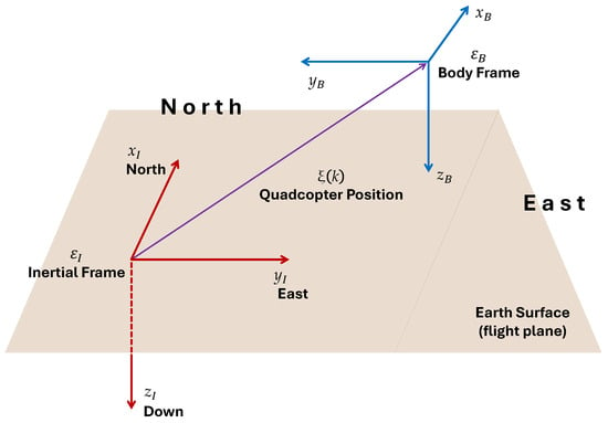
The description of the spatial movement of a quadcopter requires a dual coordinate system since the vehicle operates as a rigid body within a six-degree-of-freedom (6-DoF) space [15]. The navigation setup utilizes a local inertial reference frame that adheres to the standard North–East–Down (NED) aeronautical convention [15]. Complementarily, a body-fixed reference frame represents onboard workspace, whose origin is rigidly attached to the vehicle center of mass [15].
The geometric interaction between these systems is illustrated in Figure 1, where the flat surface represents a local tangent flight plane, establishing a flat-Earth kinematic approximation [24]. This assumption remains valid since the operational range of a quadcopter is structurally localized, rendering effects of Earth curvature and Coriolis accelerations negligible [24].
Figure 1.
Geometric relationship between local inertial frame and the body-fixed frame , illustrating instantaneous translational state vector under a flat-Earth approximation.
Within this setup, the Cartesian state defines the instantaneous position of the center of mass, operating as a time-varying vector expressed in the global reference system at discrete step k:
The spatial orientation of the body frame relative to inertial frame is determined by conventional Euler angle vector , where represents the roll angle, denotes the pitch angle and corresponds to the yaw angle [24]. However, because the external offboard routine commands translation velocities directly within the local tangent plane, complex rotational transformation matrices are governed internally and transparently by native autopilot firmware [15,25].
2.2. Translational Guidance Kinematics
Assuming a forward-Euler discretization scheme with a sampling period [24], the discrete-time translational mechanics of the quadcopter center of mass can be modeled directly within an inertial framework. This relationship maps the high-level position state updates as follows:
where represents the linear velocity control vector synthesized by the external guidance algorithm. This formulation bypasses rotational rigid-body transformations at the supervisory layer, establishing a direct kinematic foundation for the position regulation objective.
2.3. Position Regulation Objective
The control objective requires the mathematical formulation of a robust guidance scheme capable of executing precise point-to-point regulation under adverse flight conditions. The reference generator defines the target coordinates in three-dimensional space, which is represented as the desired constant position vector :
where operates as a static step command during position regulation experiments designed to evaluate transient and steady-state responses under actuator constraints [26].
The tracking error variable yields the absolute algebraic discrepancy between the active reference target and the estimated position feedback of the aircraft:
The primary task of the intelligent controller is to synthesize a bounded velocity strategy that drives the tracking error asymptotically to the origin [27]. This implies satisfying the condition for a given stationary target, ensuring high precision and rejection of environmental perturbations.
2.4. Baseline Autopilot Cascaded Control Architecture
The cascaded paradigm establishes a hierarchical structure where the inner loop directly governs the fast rotational dynamics, thereby allowing the outer loop to focus entirely on translational behavior [15,25]. In this standard configuration [18,20], the native position control loop operates as the primary stage, translating spatial deviations into local kinematic targets while bypassing low-level multirotor actuation details.
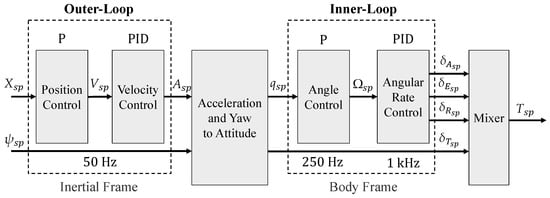
To provide a comprehensive operational overview, Figure 2 outlines the sequential signal propagation throughout the default embedded flight system.
Figure 2.
Signal propagation pipeline and multi-rate execution frequencies within the native PX4 firmware [20].
The initial translation task begins in the inertial frame, where the proportional (P) position control block processes the three-dimensional tracking error defined in the previous subsection alongside the desired yaw heading setpoint . For stable stationary regulation, this heading is maintained at a constant zero reference. This loop filters the spatial deviations to synthesize the native velocity reference vector , acting as the target input for the subsequent stages:
where its individual components define the target translational velocities along the North, East, and Down directions, respectively.
As illustrated in the control loop hierarchy depicted in Figure 2, the subsequent velocity control block utilizes a PID scheme to process these references, calculating an intermediate acceleration setpoint at a frequency of 50 Hz [20]. The firmware then executes a coordinate transition through the acceleration-and-yaw-to-attitude module, converting these translational demands into a target attitude quaternion mapped to the body-fixed at 250 Hz [20]. Within this inner loop structure, a proportional (P) angle controller computes the commanded angular rate vector , subsequently driving the high-frequency angular rate PID module operating at 1 kHz [20].
Finally, this internal rate stage outputs the normalized aerodynamic control demands for roll, pitch, yaw and thrust, which are denoted as , , and , respectively [20]. The mixer module processes these scaled variables to generate the collective motor commands transmitted to the physical electronic speed controllers [20]. The offboard control routine exploits this routing configuration by serializing its custom supervisory signals in real time into MAVLink communication packets, setting the stage for advanced tracking optimization [20].
3. Adaptive Neural PID Control with Asymmetric Saturation
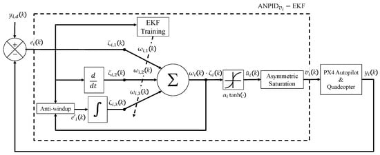
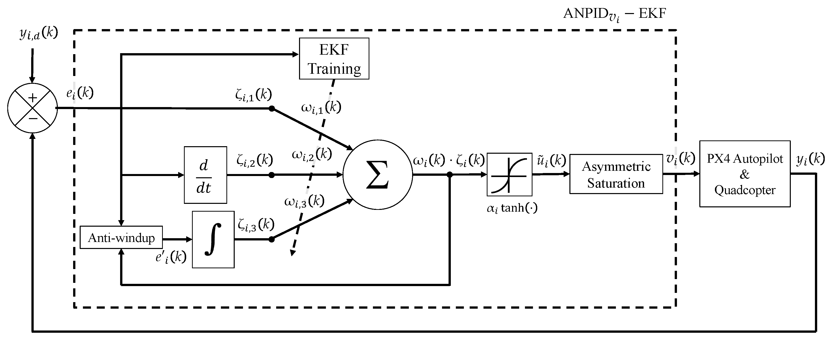
This section details the theoretical design and mathematical formulation of the proposed intelligent outer-loop guidance strategy. To establish a rigorous baseline for this framework, its foundational control paradigms are defined as follows: (i) Neural PID control expands classical tracking by substituting static gains with time-varying synaptic parameters optimized online, enabling real-time adaptation against unmodeled dynamics [14,27,28]; (ii) Asymmetric saturation dictates that signal boundaries are non-uniform and axis-dependent, preventing vector distortion when physical constraints vary across different operational domains [22,29]; (iii) Anti-windup denotes the broader class of control compensation methods designed to mitigate the transient response degradation caused by actuator or velocity saturation [22]; and (iv) Clamping, or conditional integration, is a specific anti-windup mechanism that dynamically freezes the integrator state the instant saturation is detected, eliminating residual overshoot [21]. By synthesizing these distinct principles, the proposed scheme utilizes a single-neuron architecture optimized via an Extended Kalman Filter (EKF) to safely generate bounded translational velocity commands. The block diagram of the proposed control strategy is shown in Figure 3.
Figure 3.
Block diagram of the proposed supervisory control loop for the i-th operational axis.
3.1. Single-Neuron State Mapping and Activation
The intelligent controller acts directly upon the tracking deviations expressed in the local tangent flight plane. At each discrete-time step k, the tracking error vector establishes the fundamental feedback loop. To avoid notation conflicts with standard plant states and spatial coordinates, an augmented error vector is constructed for each operational axis :
where characterizes the discrete-time backward difference derivative mapping [26]:
and denotes the unconstrained accumulation of the error channel [21,26]:
The adjustable synaptic weight vector substitutes the static proportional, derivative and integral gains of a conventional PID controller, respectively [28]. This single-neuron architecture is specifically selected over deep multi-layer networks to guarantee the deterministic low-latency execution on embedded microcontrollers and to preserve the physical interpretability of the control gains. The preliminary velocity command is computed from the inner product of the weights and the augmented error vector, which is bounded by a nonlinear activation mapping. The hyperbolic tangent function is selected to introduce nonlinearity into the neural structure. Unlike purely linear unbounded functions, this mapping provides a continuously differentiable boundary necessary to compute the EKF Jacobian without singularities, inherently restricts the maximum command amplitude, and preserves ideal linear PID behavior near the equilibrium point:
where represents the scaling parameter associated with the physical velocity limits of the multirotor system.
3.2. Extended Kalman Filter Weight Optimization
The continuous adaptation of the synaptic parameters relies on an active Extended Kalman Filter routine executing concurrently at the supervisory layer. Following a state-space formulation, the EKF treats the adjustable control gains as the state vector of an artificial dynamical system governed by a random-walk model [12,28]. The measurement update phase utilizes the tracking error to drive this online learning mechanism.
To linearize the nonlinear activation response within the estimation loop, the algorithm derives an instantaneous Jacobian via the partial differentiation of with respect to the weights:
The error covariance matrix estimates parameter uncertainty throughout the flight routine. The algorithm computes the innovation variance and the optimal time-varying Kalman gain vector using the following expressions [12,28]:
where represents the constant measurement noise variance.
The correction phase updates the active weights online by blending the Kalman allocation strategy with localized learning rates , accelerating adaptation along the gradient of the error:
where ⊙ denotes the element-wise Hadamard product. Finally, the covariance matrix is updated according to the discrete Riccati equation [12,28]:
where denotes the diagonal process-noise matrix designed to maintain continuous filter alertness [12,28]. Unlike batch-trained algorithms, this recursive estimation process does not retain historical data buffers. At each discrete time step k, exactly one newly collected measurement is incorporated to update the weights, and the sample is immediately discarded.
3.3. Asymmetric Saturation and Conditional Anti-Windup Clamping
To ensure operational safety during large setpoint steps, the control signals are conditioned through a strict directional stabilization process before transmission. Since quadcopter platforms possess asymmetric velocity constraints across different axes, conventional axis-decoupled clipping can cause severe vector distortion [15]. Consequently, the proposed strategy executes a coupled, direction-preserving saturation routine implemented across the horizontal flight plane while maintaining a separate clamping constraint for the vertical lifting mechanics [15,20].
In the horizontal domain, the saturation mechanism monitors the coupled magnitude of the forward and lateral demands. If the Euclidean norm of these translational signals exceeds the maximum velocity threshold , the preliminary commands are scaled proportionally to preserve the original guidance vector direction:
Concurrently, the vertical velocity command is restricted by a strict clamping constraint defined by the independent physical limit :
To prevent trajectory degradation caused by integral windup during saturation intervals, the single-neuron structure implements a conditional integration rule [21,29]. This accumulation process depends directly on the argument of the activation function with the integral state updated as follows:
where the filtered error variable responds to the following logical constraint:
This structural arrangement effectively freezes the integral action once the argument of the activation function indicates a saturation condition, enabling an immediate recovery without residual overshoot when the quadcopter returns to nominal tracking thresholds [21].
3.4. Parameters and Tuning Guidelines
The dynamic response and numerical stability of the scheme depend directly on the selection of parameters:
- Measurement Noise Covariance (R): sets the filter confidence regarding tracking error measurements. A small R accelerates gain adaptation but increases sensitivity to sensor noise, generating high-frequency chattering in the synthesized velocity commands. Conversely, an excessively large R slows down parameter convergence, degrading disturbance rejection under wind gusts.
- Process Noise Covariance (): dictates the parameter variation rate. Higher values preserve filter alertness against non-stationary aerodynamic forces, preventing the covariance matrix from decaying to zero. But excessively large values induce gain drift during steady-state tracking.
- Learning Rates Vector (): scales the gradient descent step along individual error channels. The proportional () and integral () rates primarily govern rise time and steady-state error compensation, while the derivative rate () provides damping against transient overshoot.
- Scaling Bounds (): restrict velocity demands to the physical limits of the multirotor platform. When tracking errors exceed these operational thresholds, the clamping logic freezes error accumulation, directly safeguarding the EKF update cycle against covariance divergence.
The initial synaptic weights are set to conservative linear PID gains to ensure stable initial hovering prior to online adaptation: and . The scaling parameters m/s and m/s are selected to match the physical kinematics of the tested quadcopter. Finally, the covariance matrices are initialized as and to balance rapid transient adaptation with steady-state noise rejection.
4. Hardware-in-the-Loop (HIL) Simulation Environment
To evaluate the proposed architecture under realistic conditions, an experimental HIL platform has been developed. This setup contrasts with Software-in-the-Loop (SITL) configurations [20,25], where environment-specific firmware runs entirely on a development computer. In HIL, standard PX4 firmware executes directly on the physical flight hardware [20,25].
The main difference between the environments lies in the data injection point [20,25]. SITL relies on simulation drivers to emulate environmental data within a software process [20]. Conversely, HIL forces core firmware modules, such as the commander and sensor suites, to initialize in a startup mode that bypasses physical drivers and accepts external telemetry streams [20]. Therefore, while SITL executes more of the standard low-level system code, HIL validates the control algorithm under the exact processing and timing constraints of the physical microcontroller [20].
4.1. Distributed Embedded Hardware and Physics Co-Simulation Layer
The configuration of the HIL setup is divided into an embedded flight computing platform, a rigid-body physics emulation workspace, and a supervisory intelligent guidance layer. The physical embedded hardware core consists of the NXP MR-VMU-RT1176 Flight Management Unit (FMU) [20]. This specialized aeronautical board integrates a high-performance dual-core crossover processor featuring an ARM Cortex-M7 core operating at 1 GHz and an ARM Cortex-M4 core operating at 400 MHz [20]. The PX4 Autopilot firmware stack (v15.1.0) executes natively within this embedded hardware layer, running high-frequency state estimation via its internal EKF2 module and governing low-level attitude tracking loops [20].
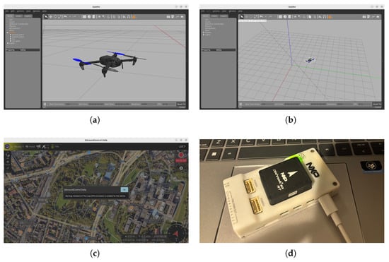
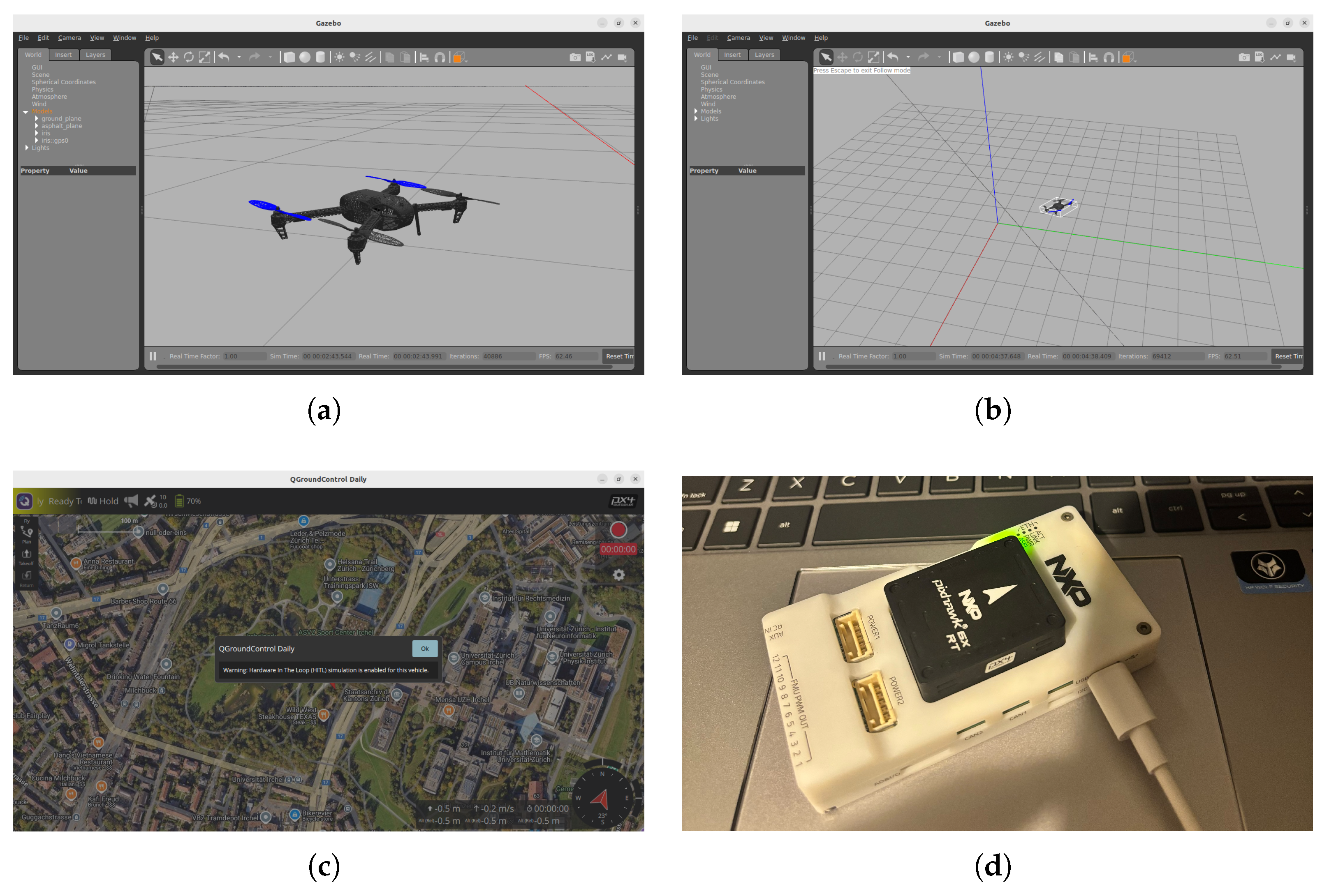
Synchronization across the physical NXP FMU and the virtual environment operates deterministically [20]: Gazebo optimizes high-rate synthetic telemetry outputs, packaging them into HIL_SENSOR and HIL_GPS MAVLink messages transmitted via a high-speed FTDI serial bridge operating at a fixed baud rate of 921,600 bps directly to the physical flight controller. The PX4 stack processes these virtual inputs as raw hardware sensor readings, solves the inner-loop attitude control action and returns the computed normalized actuator demands (HIL_ACTUATOR_CONTROLS) back to the simulator, closing the physical-virtual loop at 250 Hz to preserve real-time flight dynamics [20]. Figure 4 shows the complete layout of the components and the synchronized multi-layer simulation interfaces.
Figure 4.
Experimental platform setup: (a) Visualization of the simulated quadcopter Iris model within the Gazebo physics engine; (b) Global perspective of the flat-Earth localized tangent flight workspace inside the virtual world; (c) QGroundControl graphical user interface displaying the mandatory real-time HIL validation flag; and (d) Embedded NXP hardware platform executing the production autopilot firmware.
4.2. Asynchronous Offboard Command Loop and Telemetry Pipeline
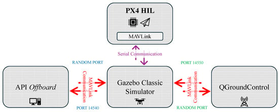
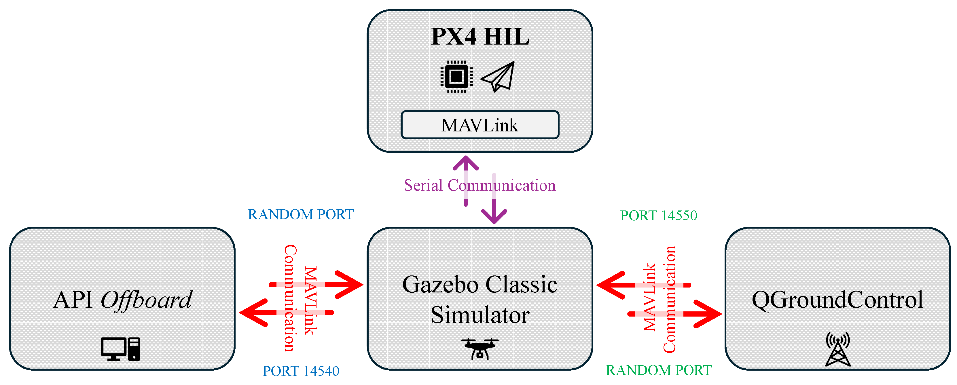
The proposed supervisory intelligent controller executes externally within an independent offboard node implemented in Python 3. Due to the high computational complexity associated with the online update process within the EKF weight optimization routine, the algorithm is deployed on the host companion workstation operating under Ubuntu 22.04 LTS, decoupling the advanced guidance loop from the low-level firmware tasks. The script utilizes the pymavlink library to establish a bidirectional telemetry and command routing interface with the PX4 flight stack via UDP socket serialization through port 14540 [20,30], as detailed in the network routing topology illustrated in Figure 5.
Figure 5.
Block diagram of the offboard communication network.
At each discrete-time step k, the offboard node blocks execution until a valid LOCAL_POSITION_NED message is received from the NXP FMU to extract the position states , and [20]. The routine then evaluates the three-dimensional tracking errors relative to the reference coordinates . Subsequently, the single-neuron mapping functions, backward derivative parameters, and conditional clamping anti-windup laws are solved for each operational channel. The resulting velocity commands are then transmitted back to the autopilot at a sampling frequency of 50 Hz ( s). Empirical testing demonstrates that higher execution frequencies (e.g., 100 Hz or 200 Hz) do not yield substantial improvements in outer-loop translational dynamics and unnecessarily saturate the MAVLink communication bus. Furthermore, 50 Hz aligns exactly with the recommended offboard setpoint injection rate specified by the PX4 architecture [20]. The internal attitude and rate controllers operate under the standard factory optimization provided by the firmware.
To explicitly clarify the computational implementation, the continuous real-time execution loop of the offboard control node is formalized in Algorithm 1.
| Algorithm 1 Real-Time Offboard Execution Loop |
|
4.3. MAVLink Bitmask Configuration for Velocity Command Injection
To inject the velocity vector generated by the single-neuron structure into the native cascaded flight software without firmware modification, the Python node utilizes the 16-bit unsigned integer bitmask (type_mask) within the SET_POSITION_TARGET_LOCAL_NED MAVLink message [20,30]. This field determines which control channels are executed by the internal loops. Following an inverse logic, setting a bit to 1 commands PX4 to bypass the corresponding tracking state, whereas a bit set to 0 activates the channel input.
The offboard routine configures the bitmask value as 3527 (0b110111000111) to isolate velocity control and bypass native position tracking [20,30]. This instructs the autopilot to disable the proportional position controllers and route the intelligent outer-loop outputs directly into the velocity PID stages, ensuring that the quadcopter response depends strictly on the neural adaptive tuning laws.
5. Results and Discussion
This section details the comprehensive performance evaluation of the proposed control scheme through rigorous HIL testing. To establish a robust scientific validation, the adaptive intelligent controller is compared directly against a baseline P controller and a conventional PID controller. Both baselines utilize the exact factory-certified tuning parameters provided by the PX4 firmware. All three control schemes are evaluated under identical initial flight conditions, physics engine step sizes, and deterministic wind disturbance seeds.
5.1. HIL Environmental Parameterization and Virtual Workspace Configuration
To evaluate transient tracking behavior, reference convergence, and actuator saturation mitigation, a representative multi-axis step response testbench is implemented within the distributed HIL workspace. The reference generator commands a simultaneous spatial step defined by the target coordinates m, enforcing a total translation of approximately m along the horizontal navigation plane and a localized 10-meter altitude ascent command executed along the negative Down direction of the local inertial frame.
The physical environment is governed by a custom virtual workspace configured within the Gazebo Classic engine via the hitl_iris_world SDF framework. The mechanical and aerodynamic properties are governed by an Open Dynamics Engine (ODE) solver executing at a maximum step size of s with a real-time update frequency of 250 Hz and a real-time factor equal to 1. The local gravity vector is parameterized as m/s2. The ODE solver constraints utilize a Constraint Force Mixing (CFM) value of 0, an Error Reduction Parameter (ERP) of 0.2, a maximum correcting velocity bound of 100 and a contact surface layer thickness of 0.001 to ensure structural simulation stability. Aerodynamic disturbances are synthesized dynamically through the libgazebo_wind_plugin.so module attached to the vehicle base_link frame.
To rigorously test the operational resilience of each controller, three independent meteorological flight scenarios are evaluated: Nominal Conditions, Moderate Wind, and Gusty Wind.
5.2. Scenario 1: Nominal Environmental Conditions (No Wind Disturbance)
The initial benchmark test evaluates the tracking capability of each framework under an ideal, disturbance-free flight profile (0 m/s). This baseline isolates the geometric tracking error from external forces, verifying the nominal transient response under the target step coordinates m. Table 2 details the quantitative performance metrics computed from the experimental code telemetry for this ideal scenario.
Table 2.
Systematic performance metrics comparison under nominal environmental conditions.
The numerical data compiled in Table 2 confirm that the proposed establishes a superior transient tracking profile even in the absence of external perturbations. In the horizontal North axis (X), the intelligent scheme achieves complete dominance across all indicators, compressing the settling time to s and reducing the maximum overshoot to compared to the exhibited by the conventional PID.
While the fixed-gain architectures present slightly tighter static metrics in isolated channels due to the absence of initial parameter adaptation transience, the neural mapping minimizes the global cumulative error, reducing the Integral Absolute Error (IAE) to m·s (X-axis) and m·s (Y-axis). This configuration validates that the stochastic learning loop introduces no high-frequency oscillations or tracking divergence under nominal conditions.
5.3. Scenario 2: Moderate Wind Conditions (Beaufort 4, 7.0 m/s)
The second flight scenario introduces a steady, continuous crosswind classified as Beaufort 4 (moderate breeze) targeting the step reference coordinates m [31,32]. The wind plugin parameters describe a baseline tridirectional force defined by a mean velocity m/s, a maximum threshold m/s and a magnitude variance . The spatial alignment follows a normalized tridirectional entry vector with a directional angular variance of , inducing continuous turbulence variations of . Table 3 details the quantitative performance metrics computed from the experimental code telemetry.
Table 3.
Systematic performance metrics comparison under Beaufort 4 crosswind conditions.
When continuous aerodynamic disturbances are introduced, fixed-gain architectures suffer from significant performance degradation. As compiled in Table 3, the maximum overshoot in the horizontal plane expands drastically for the baseline controllers with the proportional reaching an overshoot of in the X-axis and the conventional PID reaching .
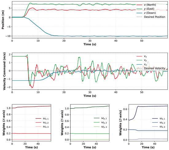
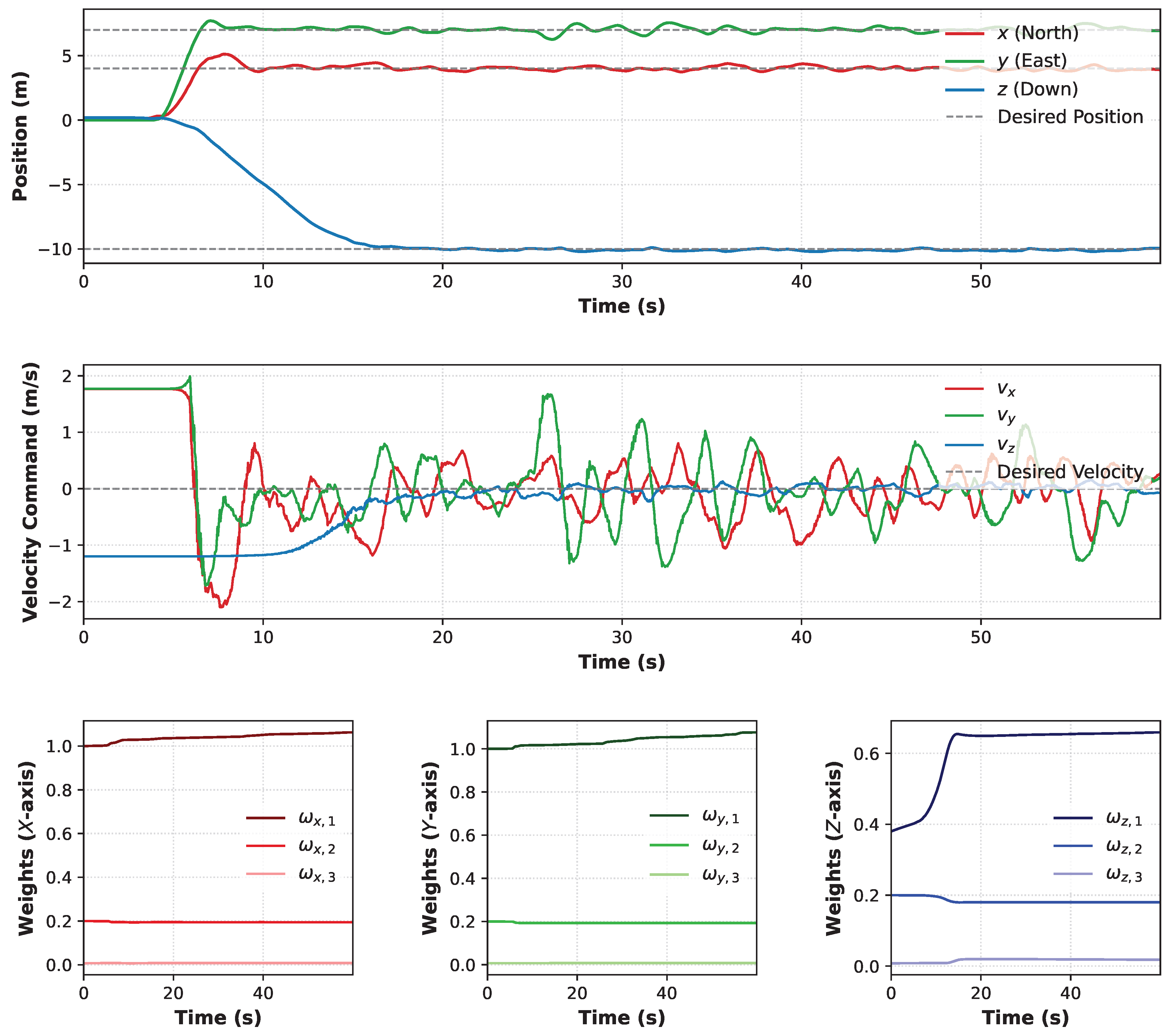
Conversely, the proposed successfully restrains this transient deviation to (X-axis) and (Y-axis). This optimal response confirms that the conditional clamping anti-windup integration loop effectively prevents integral saturation by isolating the error state variables during saturation periods. The online tuning optimization reduces the settling time to s (X-axis) and s (Y-axis), enabling the vehicle to acquire the localized step coordinates faster than the conventional baselines. This complete physical interaction, along with the internal parameter update history, is detailed in Figure 6, showcasing how the synaptic layers reach multi-axis stochastic stability.
Figure 6.
Operational transient responses and parameters update profile of the proposed scheme under Moderate Wind. The top panel illustrates the multi-axis spatial positions tracking relative to the coordinate reference; the middle panel presents the synthesized local velocity command vectors (); and the bottom panels detail the autonomous stochastic convergence of the internal synaptic weight layers across each individual navigational channel.
5.4. Scenario 3: Gusty Wind Conditions (Beaufort 6, 8–14 m/s)
The final and most critical flight experiment subjects the quadcopter to severe atmospheric turbulence corresponding to Force 6 on the Beaufort Scale [31,32] under the target coordinates m. To ensure proper sensor initialization and prevent gyroscope calibration failures within the PX4 firmware stack during the system boot sequence, the simulation environment launches under near-calm nominal conditions ( m/s). The comprehensive, multi-directional strong wind profile is subsequently introduced through the transient gust parameterization framework, which is programmed to trigger precisely at s with a continuous execution duration of s.
This atmospheric burst injects a mean velocity step increment of m/s, bounding the localized operating environment between m/s and m/s, with an internal stochastic turbulence variance configured at . The spatial propagation vector of the gust targets a unidirectional horizontal alignment along the positive East axis (). Table 4 summarizes the performance parameters extracted over the entire flight profile.
Table 4.
Systematic performance metrics comparison under gusty wind conditions, Beaufort 6.
5.5. Methodological Analysis of Non-Stationary Disturbances and Performance Trade-Offs
A critical analytical distinction must be established when interpreting the numerical data from Scenario 3. Under highly non-stationary and stochastic wind fields triggered mid-flight ( s), traditional global metrics such as the Settling Time () and Maximum Overshoot () lose part of their conventional deterministic meaning. Because these parameters convolute the initial step response with the subsequent aerodynamic impact, they must be analyzed in combination with cumulative deviation tracking criteria. In cascaded commercial autopilots, unhandled actuator saturation manifests as severe integral windup. Therefore, and IAE serve as the primary quantitative indicators of saturation mitigation.
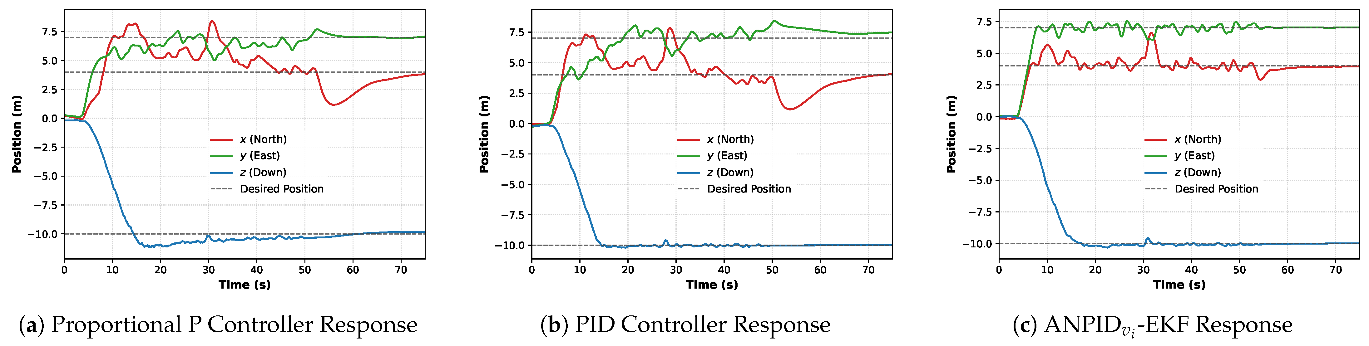
For instance, while the conventional PID controller yields a slightly lower global settling time in the X-axis ( s) and tighter regulation along the vertical Z-axis, it exhibits severe path degradation and drift when the wind burst strikes, as evidenced by the high IAE values ( m·s and m·s) in the horizontal plane.
Considerable structural survival and resilience are provided by the proposed , which compresses the Mean Squared Error (MSE) in the North axis to m2 and restricts the maximum overshoot to compared to the catastrophic overshoot generated by the proportional baseline.
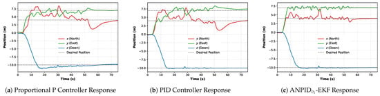
In the East axis (Y), which receives the horizontal perpendicular impact of the gust directly, the proposed controller isolates the cross-axis error completely, minimizing the IAE to m·s and settling the vehicle in just s. This performance confirms that the intelligent layer adapts its tracking behavior on the fly, outperforming classical fixed-gain structures under extreme meteorological transitions. The resulting multi-axis translation responses for all three evaluated control schemes are compared side by side in Figure 7, highlighting the flight path deviations caused by the non-stationary atmospheric burst.
Figure 7.
Response profiles under Scenario 3 (Severe Beaufort 6 Gusty Wind). The transient curves illustrate the spatial regulation capabilities and path variations of each control architecture against stochastic crosswind forces introduced at s.
6. Conclusions
This paper presents an adaptive outer-loop neural PID control framework for autonomous quadrotor position regulation on a conventional PX4 flight stack within a distributed HIL configuration. The proposed controller combines a cascaded PID structure with the online adaptation capability of neural networks, granting continuous adjustment of the outer-loop gains based on an instantaneous tracking error.
The suggested methodology is experimentally validated throughout different scenarios on an HIL platform integrating Gazebo, PX4 and Pixhawk hardware, providing scenarios that closely resemble real flight while maintaining repeatability and operational safety, especially the last scenario, which accounts for wind conditions. Experimental results show that the adaptive neural outer-loop controller improves trajectory-tracking performance in comparison to the conventional P and PID fixed-gain PX4 position controllers, which are the industry baselines.
Overall, the proposed adaptive neural PID outer loop offers a practical alternative for enhancing commercial UAV flight performance through online gain adaptation while preserving the modularity of standard autopilot architectures.
Further studies will focus on trajectory tracking, disturbance rejection, adaptive payload compensation, and fully autonomous outdoor flight experiments.
Author Contributions
Conceptualization, J.O.E. and J.D.R.; methodology, J.O.E. and J.D.R.; software, J.O.E.; validation, J.O.E., J.D.R. and A.Y.A.; formal analysis, J.O.E., J.D.R. and A.Y.A.; investigation, J.O.E.; resources, J.D.R. and A.Y.A.; data curation, J.O.E.; writing—original draft preparation, J.O.E. and J.D.R.; writing—review and editing, J.O.E., J.D.R. and A.Y.A.; visualization, J.O.E.; supervision, J.D.R. and A.Y.A.; project administration, J.D.R. and A.Y.A.; funding acquisition, A.Y.A. All authors have read and agreed to the published version of the manuscript.
Funding
The authors thank the Universidad de Guadalajara for giving us the support to develop this research.
Institutional Review Board Statement
Not applicable.
Informed Consent Statement
Not applicable.
Data Availability Statement
The original contributions presented in this study are included in the article. Further inquiries can be directed to the corresponding author.
Conflicts of Interest
The authors declare no conflicts of interest.
Abbreviations
The following abbreviations are used in this manuscript:
| ANN | Artificial Neural Network |
| CFM | Constraint Force Mixing |
| DoF | Degree of Freedom |
| EKF | Extended Kalman Filter |
| EKF2 | Extended Kalman Filter 2 |
| FMU | Flight Management Unit |
| FTDI | Future Technology Devices International |
| HIL | Hardware-in-the-Loop |
| IAE | Integral Absolute Error |
| LQR | Linear Quadratic Regulator |
| LMPC | Linear Model Predictive Control |
| MAVLink | Micro Air Vehicle Link |
| MSE | Mean Squared Error |
| NED | North–East–Down |
| ODE | Open Dynamics Engine |
| PID | Proportional–Integral–Derivative |
| PX4 | PX4 Autopilot |
| SDF | Simulation Description Format |
| SITL | Software-in-the-Loop |
| SMC | Sliding Mode Control |
| STD | Standard Deviation |
| UAV | Unmanned Aerial Vehicle |
| UDP | User Datagram Protocol |
| VTOL | Vertical Take-Off and Landing |
References
- Mohsan, S.A.H.; Othman, N.Q.H.; Li, Y.; Alsharif, M.H.; Khan, M.A. Unmanned Aerial Vehicles (UAVs): Practical Aspects, Applications, Open Challenges, Security Issues, and Future Trends. Intell. Serv. Robot. 2023, 16, 109–137. [Google Scholar] [CrossRef] [Scilit] [PubMed]
- Teixeira, K.; Miguel, G.; Silva, H.S.; Madeiro, F. A Survey on Applications of Unmanned Aerial Vehicles using Machine Learning. IEEE Access 2023, 11, 117582–117621. [Google Scholar] [CrossRef] [Scilit]
- Hassanalian, M.; Abdelkefi, A. Classifications, Applications, and Design Challenges of Drones: A Review. Prog. Aerosp. Sci. 2017, 91, 99–131. [Google Scholar] [CrossRef] [Scilit]
- Shakhatreh, H.; Sawalmeh, A.H.; Al-Fuqaha, A.; Dou, Z.; Almaita, E.; Khalil, I.; Othman, N.S.; Khreishah, A.; Guizani, M. Unmanned Aerial Vehicles (UAVs): A Survey on Civil Applications and Key Research Challenges. IEEE Access 2019, 7, 48572–48634. [Google Scholar] [CrossRef] [Scilit]
- Sadi, M.A.; Jamali, A.; Kamaruddin, A.M.N.A. Optimizing UAV Performance in Turbulent Environments Using Cascaded Model Predictive Control Algorithm and Pixhawk Hardware. J. Braz. Soc. Mech. Sci. Eng. 2025, 47, 396. [Google Scholar] [CrossRef] [Scilit]
- Ogata, K. Modern Control Engineering, 5th ed.; Prentice Hall: Upper Saddle River, NJ, USA, 2010. [Google Scholar]
- Zhou, K.; Doyle, J.C.; Glover, K. Robust and Optimal Control; Prentice Hall: Upper Saddle River, NJ, USA, 1996. [Google Scholar]
- Rawlings, J.B.; Mayne, D.Q.; Diehl, M.M. Model Predictive Control: Theory, Computation, and Design, 2nd ed.; Nob Hill Publishing: Madison, WI, USA, 2024. [Google Scholar]
- Khalil, H.K. Nonlinear Systems, 3rd ed.; Prentice Hall: Upper Saddle River, NJ, USA, 2002. [Google Scholar]
- Zhang, X.; Li, X.; Wang, K.; Lu, Y. A Survey of Modelling and Identification of Quadrotor Robot. Abstr. Appl. Anal. 2014, 2014, 320526. [Google Scholar] [CrossRef] [Scilit]
- Haykin, S. Neural Networks and Learning Machines, 3rd ed.; Prentice Hall: Upper Saddle River, NJ, USA, 2009. [Google Scholar]
- Rios, J.D.; Alanis, A.Y.; Lopez-Franco, C.; Arana-Daniel, N.; Sanchez, E. Neural Networks Modeling and Control: Applications for Unknown Nonlinear Delayed Systems in Discrete-Time; Elsevier: Amsterdam, The Netherlands, 2020. [Google Scholar] [CrossRef] [Scilit]
- Gómez-Avila, J.; López-Franco, C.; Alanis, A.Y.; Arana-Daniel, N. Control of Quadrotor using a Neural Network based PID. In Proceedings of the 2018 IEEE Latin American Conference on Computational Intelligence (LA-CCI), Guadalajara, Mexico, 7–9 November 2018; pp. 1–6. [Google Scholar] [CrossRef] [Scilit]
- Gomez-Avila, J.; Lopez-Franco, C.; Alanis, A.Y.; Arana-Daniel, N. Neural PD Controller for an Unmanned Aerial Vehicle. Algorithms 2020, 13, 226. [Google Scholar] [CrossRef] [Scilit]
- Lopez-Sanchez, I.; Moyrón, J.; Moreno-Valenzuela, J. Adaptive Neural Network-Based Trajectory Tracking Outer Loop Control for a Quadrotor. Aerosp. Sci. Technol. 2022, 129, 107847. [Google Scholar] [CrossRef] [Scilit]
- Song, X.; Wu, C.; Song, S.; Stojanovic, V.; Tejado, I. Fuzzy Wavelet Neural Adaptive Finite-Time Self-Triggered Fault-Tolerant Control for a Quadrotor Unmanned Aerial Vehicle with Scheduled Performance. Eng. Appl. Artif. Intell. 2024, 131, 107832. [Google Scholar] [CrossRef] [Scilit]
- Song, X.; Wu, C.; Dong, Y.; Song, S.; Shi, H.; Zhu, J.; Yan, B.; Wu, Q. Distributed Optimal Fuzzy Adaptive Prescribed-Time Formation Control for MQUAVs with Flexible Global Quantitative Behaviors. Sci. China Technol. Sci. 2026, 69, 1100313. [Google Scholar] [CrossRef] [Scilit]
- Meier, L.; Honegger, D.; Pollefeys, M. PX4: A Node-Based Multithreaded Open Source Robotics Framework for Deeply Embedded Platforms. In Proceedings of the 2015 IEEE International Conference on Robotics and Automation (ICRA), Seattle, WA, USA, 26–30 May 2015; IEEE: New York, NY, USA, 2015; pp. 6235–6240. [Google Scholar] [CrossRef] [Scilit]
- DJI. DJI Onboard SDK. Available online: https://developer.dji.com/onboard-sdk/ (accessed on 20 August 2026).
- PX4 Development Team. PX4 User Guide. Available online: https://docs.px4.io/main/en/ (accessed on 7 July 2026).
- Åström, K.J.; Hägglund, T. Advanced PID Control; ISA—The Instrumentation, Systems, and Automation Society: Durham, NC, USA, 2006. [Google Scholar]
- Horla, D. Static Anti-Windup Compensator Based on BMI Optimization for Discrete-Time Systems with Directional Change in Controls Avoidance. Bull. Pol. Acad. Sci. Tech. Sci. 2024, 72, e151046. [Google Scholar] [CrossRef] [Scilit]
- Alanis, A.Y. Exploring Kalman Filtering Applications for Enhancing Artificial Neural Network Learning. Algorithms 2025, 18, 587. [Google Scholar] [CrossRef] [Scilit]
- Beard, R.W.; McLain, T.W. Small Unmanned Aircraft: Theory and Practice; Princeton University Press: Princeton, NJ, USA, 2012. [Google Scholar]
- Aliane, N. A Survey of Pixhawk/PX4 Autopilot and Its Impact on Research and Education. Comput. Mater. Contin. 2026, 87, 6. [Google Scholar] [CrossRef] [Scilit]
- Franklin, G.F.; Powell, J.D.; Emami-Naeini, A. Feedback Control of Dynamic Systems, 8th ed.; Pearson: New York, NY, USA, 2019. [Google Scholar]
- Jagannathan, S.; Jagannathan, S. Neural Network Control of Nonlinear Discrete-Time Systems; CRC Press: Boca Raton, FL, USA, 2009. [Google Scholar]
- Hernandez-Barragan, J.; Rios, J.D.; Alanis, A.Y.; Lopez-Franco, C.; Gomez-Avila, J.; Arana-Daniel, N. Adaptive Single Neuron Anti-Windup PID Controller Based on the Extended Kalman Filter Algorithm. Electronics 2020, 9, 636. [Google Scholar] [CrossRef] [Scilit]
- Borase, R.P.; Maghade, D.K.; Sondkar, S.Y.; Pawar, S.N. A Review of PID Control, Tuning Methods and Applications. Int. J. Dyn. Control 2021, 9, 818–827. [Google Scholar] [CrossRef] [Scilit]
- MAVLink. MAVLink Developer Guide. Available online: https://mavlink.io/en/ (accessed on 1 September 2026).
- National Weather Service (NOAA). National Weather Service. Available online: https://www.weather.gov (accessed on 20 August 2026).
- Royal Meteorological Society. Beaufort Wind Scale. Available online: https://www.rmets.org/metmatters/beaufort-wind-scale (accessed on 20 August 2026).

Disclaimer/Publisher’s Note: The statements, opinions and data contained in all publications are solely those of the individual author(s) and contributor(s) and not of MDPI and/or the editor(s). MDPI and/or the editor(s) disclaim responsibility for any injury to people or property resulting from any ideas, methods, instructions or products referred to in the content. |
© 2026 by the authors. Licensee MDPI, Basel, Switzerland. This article is an open access article distributed under the terms and conditions of the Creative Commons Attribution (CC BY) license.