Pumping Power Reduction in Crude-Oil Pipeline Transportation: CFD Validation and Kolmogorov–Arnold Network Surrogate Modelling

Abstract

Precise prediction of pressure drop and drag-reduction performance is essential for improving the hydraulic efficiency and reducing the energy demand of crude-oil pipeline transportations. Therefore, this study aims to develop an integrated computational fluid dynamics (CFD)–machine learning (ML) framework for predicting pressure drop (∆p), drag reduction (DR), pumping power reduction (PPR), energy savings (ES), and flow-rate enhancement (Q) in turbulent crude-oil pipeline flow containing drag-reducing agents (DRAs). The investigated system considers the effect of pipeline length (L), diameter (D), surface roughness (ε), operating temperature (T), and DRA concentration (25–200 ppm). The Reynolds-average Navier–Stokes equations (RANS) were solved using the shear stress transport (SST) k-ω turbulence model approaching near-wall resolution of y⁺ ≈ 1 for DRA3 at 20 ppm. The CFD modelling was first used to validate an experimental benchmark and subsequently used to expand the available dataset over the investigated operating conditions. The combined experimental–CFD dataset was then employed to develop a multi-output Kolmogorov–Arnold network (KAN) surrogate model. The proposed framework predicted DR up to 44.2%, PPR of approximately 55 W, ES of 30%, and flow-rate enhancement up to 5–10(${\displaystyle \frac{\mathrm{L}}{\mathrm{d}\mathrm{a}\mathrm{y}}}$). The KAN model effectively captured the nonlinear relationships among DRA characteristics, pipeline geometry, and operating conditions, achieving R² = 0.9318 for PPR prediction. The novelty of the proposed work lies in integrating a validated, near-wall-resolved SST k-ω CFD model with a multi-output KAN surrogate model, combining physics-based flow analysis with rapid data-driven prediction of hydraulic and energy-performance indicators.

1. Introduction

Pipeline transportation has proven to be the preferred method for transportation at remote locations (i.e., petrol, diesel, crude oil, etc.) because it offers greater cost-effectiveness and reliability than traditional tankers and haul truck systems [1]. Crude oil transportation has become a critical component of the global energy infrastructure, where operational costs and energy consumption are key considerations [2]. A pipeline’s flow behavior is predominantly controlled by the interplay of pressure gradients and gravitational forces. The associated pressure drop constitutes a critical performance parameter, directly influencing both the pumping power (PP) and operational efficacy [3,4]. Turbulent-flow pumping power reduction (PPR) and drag minimization are common goals for many different applications, such as oil and gas transportation, central heating, and commercial distribution of oil and gas off-site.

To overcome these challenges, it is essential to be aware of how turbulent flow induces drag in order to reduce it to a minimum level [5], while understanding the turbulent flow behavior of fluid flow in process engineering interactions is a key problem, particularly for flows involving non-Newtonian fluids. The precise prediction of turbulent shear stress and wall velocity gradients in pipes is important in ensuring efficient design, optimization, and operational analysis of pipe flow systems [3]. The velocity gradient and profile near the wall are the key factors for designing effective pipeline systems, precisely predicting drag, and streamlining multivariable fluid-related engineering operations. It explains how velocity changes across the length of the pipe and flow domain influence the transport of mass, momentum, energy, and complete flow dynamics [6].

Furthermore, the interconnection of the asphaltene–paraffin framework has emerged as a significant challenge for reducing pressure losses and energy consumption in crude oil transportation. Researchers [7] have produced bio-based DRAs which were synthesized enzymatically. Their outcomes improved the transportation of heavy oil by creating a stable oil-in-water (O/W) emulsion. With a low concentration of 100${\displaystyle \frac{\mathrm{m}\mathrm{g}}{\mathrm{L}}}$, viscosity was lowered by almost 70%, and the drag reduction (DR) reached 40% for light crude oil inside the pipeline. They demonstrated real-field applications of these bio-based DRAs in a pipeline 6.3 km in length and 0.219 m in diameter at the well-known Daqing Oilfield. Based on experimental observations, their study offers a pathway for potential energy savings (ES) and reduced operational costs.

Contemporary developments in drag-reducing agents (DRAs) highlight their capability to optimize crude oil transportation through pipelines. Coupled with flow direction adjustments, these agents contribute to a measurable reduction in pressure drop (∆p), directly impacting energy efficiency and operational effectiveness. The numerous studies in this area have been largely driven by the significant drag reduction achieved by minute concentrations of large polymer chain polymers to Newtonian turbulent flows [8,9]. This effect has strong practical importance because it can substantially lower pumping energy requirements and operating costs in agriculture and industrial fluid-transport systems. The use of DRAs has emerged as a robust approach for alleviating frictional resistance in turbulent pipeline flows, concurrently lowering operational costs and pumping power, increasing flow rates, and hence significantly optimizing flow performance [10,11].

Recent developments integrating advanced polymers with non-additives have demonstrated significant insights in enhancing the durability and efficacy of drag-reducing agents (DRAs) under variable flow regimes, effectively addressing fundamental issues including degradation of monomer chains, reusability, and operational variability at different locations in pipelines, in minute amounts, and at various velocities [12]. But experimental investigations into pipeline transport have consistently highlighted challenges associated with pressure drop (∆p), including turbulence-induced friction, flow instabilities, and polymer degradation under varying operational conditions [13]. Over the past few decades, CFD has overcome the experimental challenges by adopting turbulence reduction models at comprehensive levels [14]. Hence, employing CFD turbulence models enables the design of DRA formulations specifically tailored to pipeline geometries and fluid properties. This innovative approach not only mitigates frictional losses but also facilitates substantial energy savings, reduces environmental impacts, and enhances overall flow efficiency [15]. Continuous research into these technologies is essential to further refine their application in complex multiphase flows, ultimately supporting a significantly more efficient and environmentally responsible future in crude-oil pipeline transport [16].

Recent work highlights the role of DRAs in reducing pressure drop and improving flow characteristics in crude and product oil pipelines, but many studies remain largely empirical or limited to base simulation comparisons without rigorous CFD-based physics-informed analysis under varied operational regimes [14,15]. Furthermore, investigations into the nonlinear interactions among DRA concentrations (ppm), Reynolds numbers (Re), and pipeline conditions (i.e., temperature, flow rate, roughness, etc.) are scarce, and computational frameworks integrating turbulence effects with predictive modelling remain limited [17,18,19].

As a result, systematic, data-driven approaches to evaluate and optimize DRA performance in long-distance crude-oil pipelines are still lacking, particularly those that can provide both predictive accuracy and physical interpretability.

The objectives of the present work are (1) to reduce the pumping power (PP), pressure drop (∆p), and drag reduction (DR) and validate them against experimental benchmarks in non-Newtonian turbulent crude-oil flow by using an SST k-ω-based CFD framework; and (2) to develop and independently evaluate a KAN-based surrogate multi-output regression model for predicting the experimentally supported output variables (∆p, DR, and PPR).

The novelty of this study lies in developing an integrated CFD–machine learning coupled framework involving (1) a validated SST k-ω turbulence model to resolve near-wall turbulence (y⁺ ≤ 1), shear stress transport, pressure losses, and PPR in DRA-assisted crude-oil pipelines, providing a unified assessment of PPR; and (2) a KAN model developed and tested for prediction performance to capture the nonlinear effects of polymer characteristics (concentration and nature) and pipe flow dynamics (length, diameter, and operating conditions).

2. Governing Equations

2.1. Continuity Equation

Equation (1) represents conservation of mass in the flow. The first term represents local density change, and the second term represents the convective transport of mass [20]:

$${\displaystyle \frac{\partial \mathsf{\rho }}{\partial t}}+\nabla \cdot \left(\mathsf{\rho }u\right)=0\hspace{1em}$$

(1)

For incompressible fluid flow (e.g., water and polymers), the above equation ($\mathsf{\rho }$ = constant) reduces to:

$$\nabla \cdot u=0$$

(2)

where

ρ is the fluid density (${\displaystyle \frac{\mathrm{k}\mathrm{g}}{{\mathrm{m}}^3}}$);

t is time of fluid flow (s);

u is the fluid velocity (${\displaystyle \frac{\mathrm{m}}{\mathrm{s}}}$);

∇ is the divergence operator.

2.2. Navier–Stokes Equation

Turbulent flow is characterized by fluctuating velocities and is written as follows;

$$u=\overline{u}+\acute{u}$$

(3)

where $\overline{u }$ is the time-averaged mean velocity, (${\displaystyle \frac{\mathrm{m}}{\mathrm{s}}}$); $\acute{u}$ is the fluctuating velocity, (${\displaystyle \frac{\mathrm{m}}{\mathrm{s}}}$).

Equation (4) governs momentum conservation [21,22]. The left-hand term, $\rho \left({\displaystyle \frac{\partial u}{\partial t}}+\left(u.\nabla \right)u\right)$, accounts for local and convective acceleration, while the right-hand side, $\left(-{\nabla }^2\mathrm{p}+\mu {\nabla }^{2}u+F\right)$, accounts for pressure forces, viscous forces, and external body forces (i.e., gravity).

$$\mathsf{\rho }\left({\displaystyle \frac{\partial u}{\partial t}}+\left(u\cdot \nabla \right)u\right)=-{\nabla }^{2}p+\mathsf{\mu }{\nabla }^{2}u+F$$

(4)

where ρ is the fluid density (${\displaystyle \frac{\mathrm{k}\mathrm{g}}{{\mathrm{m}}^3}}$); u is the fluid velocity, (${\displaystyle \frac{\mathrm{m}}{\mathrm{s}}}$); p is the pressure, (Pa); μ is the dynamic viscosity, (Pa.s); and F is the body force, (${\displaystyle \frac{\mathrm{N}}{{\mathrm{m}}^3}}$).

Substituting Equation (3) into Equation (4) gives Equation (5), which shows that turbulent stresses are the key complexity in modelling turbulent pipe flow:

$$\mathsf{\rho }\left({\displaystyle \frac{\partial \overline{u}}{\partial t}}+\left(\overline{u}\cdot \nabla \right)\overline{u}\right)=-{\nabla }^{2}p+\mathsf{\mu }{\nabla }^2\overline{u}-\mathsf{\rho }\nabla \cdot \overline{\acute{u\stackrel{´}{u}}}+F\hspace{1em}$$

(5)

where ρ is the fluid density (${\displaystyle \frac{\mathrm{k}\mathrm{g}}{{\mathrm{m}}^3}}$); $\overline{u}$ is the average velocity, (${\displaystyle \frac{\mathrm{m}}{\mathrm{s}}}$); p is the pressure, (Pa); $\acute{u}$ is the fluctuating velocity, (${\displaystyle \frac{\mathrm{m}}{\mathrm{s}}}$); and F is the body force, (${\displaystyle \frac{\mathrm{N}}{{\mathrm{m}}^3}}$).

2.3. Viscoelastic Models for Polymer Drag Reduction (DR %)

Momentum Equation with Polymer Extra Stress

Equation (6) presents the momentum equation with the polymer extra stress term [23]:

$$\mathsf{\rho }\left({\displaystyle \frac{\partial u}{\partial t}}+u\cdot \nabla u\right)=-\nabla p+\nabla \cdot \left(2{\mathsf{\eta }}_{s}D+{\mathsf{\tau }}_p\right)$$

(6)

$$D={\displaystyle \frac{1}{2}}\left(\nabla u+{\left(\nabla u\right)}^T\right)$$

(7)

where $\rho$ is the fluid density, (${\displaystyle \frac{\mathrm{k}\mathrm{g}}{{\mathrm{m}}^3}}$); $u$ is the fluid velocity, (${\displaystyle \frac{\mathrm{m}}{\mathrm{s}}}$); p is the pressure, (${\displaystyle \frac{\mathrm{N}}{{\mathrm{m}}^2}}$); ${\mathsf{\eta }}_s$ is solvent dynamic viscosity, (${\displaystyle \frac{\mathrm{k}\mathrm{g}}{\mathrm{m}\mathrm{s}}}$); $D$ is the rate of strain tensor, (${\displaystyle \frac{1}{\mathrm{s}}}$); and ${\mathsf{\tau }}_p$ is the polymer extra stress tensor, (Pa).

During the numerical solution, the momentum equation is discretized over each computational control volume and solved iteratively with the pressure–velocity coupling algorithm. The velocity, pressure, and polymer-stress fields are successfully updated until the specified residual convergence criteria and stable monitored values of pressure drop and velocity are achieved.

2.4. Power-Law Rheological Model

PEO solution with water exhibits non-Newtonian shear-thinning behavior. Hence, the polymer solutions <1 usually indicate shear-thinning behavior, where viscosity decreases with increasing shear rate, are well treated with the Power-Law Rheological Model [24]. This model effectively represents the viscosity reduction of PEO solution under increased shear rate during turbulent flow.

$$\mathsf{\tau }=K\dot{{\mathsf{\gamma }}^n}$$

(8)

$${\mathsf{\mu }}_{app}=K\mathsf{\gamma }\dot{}(\mathrm{n}-1)$$

(9)

where $\mathsf{\tau }$ is the shear stress, (Pa); $K$ flow consistency index; $\mathsf{\gamma }\dot{}$ is the shear rate, (${\displaystyle \frac{1}{\mathrm{s}}}$); and $\mathrm{n}$ is the flow behavior index.

In the numerical procedure, the local shear rate is obtained from the calculated velocity-gradient field, after which the apparent viscosity is updated in every computational cell. The momentum equation is then resolved using the updated viscosity, and this iterative process continues until both the rheological properties and the flow variables reach convergence.

3. Turbulence Models

3.1. Direct Numerical Simulation (DNS)

In this approach, it is possible to resolve all fluctuations in the flow. However, this approach requires a sufficiently refined computational grid and an extremely small timestep [25]. The complexity of these requirements escalates with the increase in the Reynolds number. In practice, this approach is limited to research applications involving low-Reynolds-number flows and is confined to supercomputing resources. Consequently, its applications to real-world, high-Reynolds-number flows remain impractical with current computational capabilities. The Navier–Stokes equation is given as follows:

$${\displaystyle \frac{\partial u}{\partial t}}+\left(u\cdot \nabla \right)u=-{\displaystyle \frac{1}{\mathsf{\rho }}}\nabla p+\mathsf{\nu }{\nabla }^{2}u+F$$

(10)

where u is the fluid velocity (${\displaystyle \frac{\mathrm{m}}{\mathrm{s}}}$); t is the time, (s); p is the pressure, (Pa); $\rho$ is the fluid density, (${\displaystyle \frac{\mathrm{k}\mathrm{g}}{{\mathrm{m}}^3}}$); $\nu$ is the kinematics viscosity, (${\displaystyle \frac{{\mathrm{m}}^2}{\mathrm{s}}}$); and $F$ is the body force (N).

3.2. Reynolds-Averaged Navier–Stokes (RANS)

This model is widely used by engineers in the industry to deal with turbulent flow losses and energy dissipation rates. Various turbulence models (i.e., Spalart–Allmaras (1 equation), k-ε, k-ω, transition k-kl-omega (3-equation), SST k-ω (2 equation), etc.) are used to deal with turbulent flow [26]. All the equations are resolved to analyze the time-averaged flow characteristics and quantify the turbulence fluctuations. A comprehensive comparison of all turbulence models is given in Table 3.

3.3. Shear Stress Transport (SST k-ω) 2-Equation Model

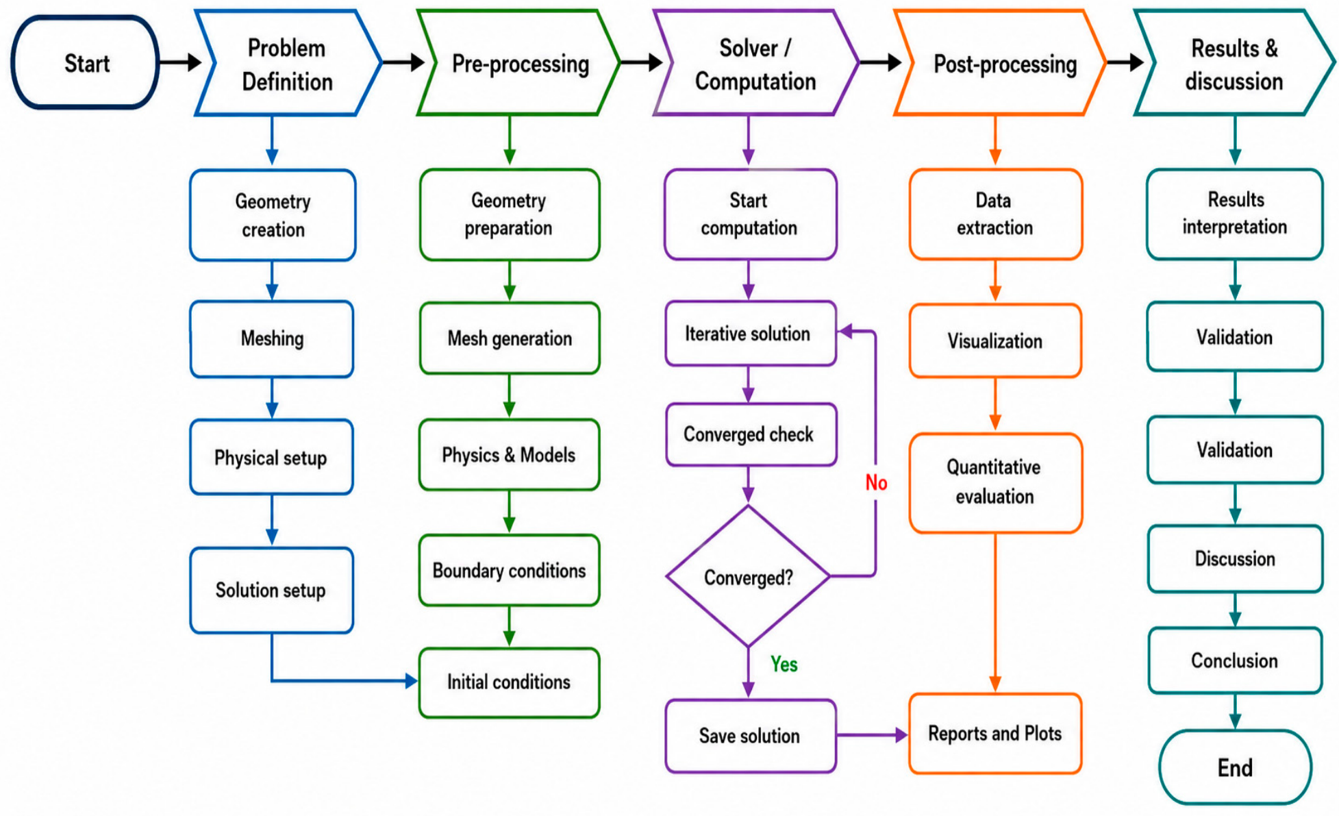
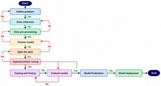
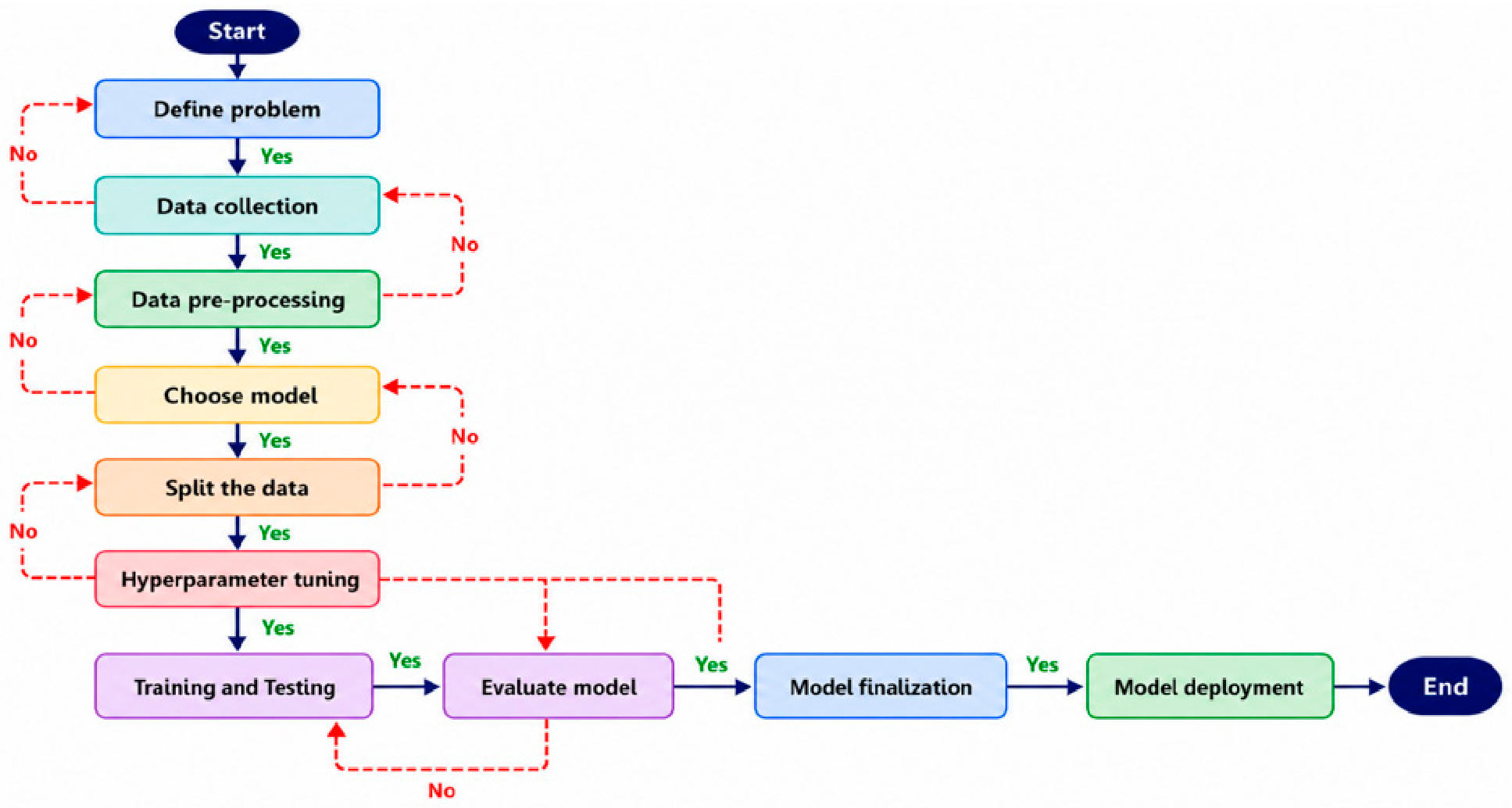
The Shear Stress Transport (SST k-ω) 2-equation model combines the standard k-ω formulation near walls with the k-ε formulation in the free stream using a blending function, providing robust prediction of adverse pressure gradients and separation [27]. Figure 1 shows the numerical flowchart for pumping power reduction (PPR) by using various steps of numerical simulation.

3.3.1. Turbulent Kinetic Energy (k) Equation

Equation (11) presents the kinetic energy transport equation, which describes the evolution of turbulent kinetic energy (k) in the flow involving a polymer solution. This reflects the work presented in [28,29,30], as given below:

$${\displaystyle \frac{\partial \left(\mathsf{\rho }k\right)}{\partial t}}+{\displaystyle \frac{\partial \left(\mathsf{\rho }k{\mathit{u}}_{\mathit{i}}\right)}{\partial x_i}} ={\displaystyle \frac{\partial }{\partial x_j}}\left[\left(\mathsf{\mu }+{\mathsf{\sigma }}_k{\mathsf{\mu }}_t \right){\displaystyle \frac{\partial k}{\partial x_j}}\right] +P_k-{\mathsf{\beta }}^{*}\rho k\omega$$

(11)

where $\rho$ is the fluid density, (${\displaystyle \frac{\mathrm{k}\mathrm{g}}{{\mathrm{m}}^3}}$); $k$ is the turbulent kinetic energy, (${\displaystyle \frac{{\mathrm{m}}^2}{{\mathrm{s}}^2}}$); $u_i$ is the fluid velocity, (${\displaystyle \frac{\mathrm{m}}{\mathrm{s}}}$); $\mathsf{\mu }$ is the kinematics viscosity, (${\displaystyle \frac{\mathrm{k}\mathrm{g}}{\mathrm{m}\mathrm{s}}}$); $P_k$ is the production of turbulent kinetic energy, (${\displaystyle \frac{\mathrm{k}\mathrm{g}}{\mathrm{m}{\mathrm{s}}^3}}$); $\mathsf{\beta }$ is the model constant; and $\omega$ is the specific dissipation rate, (${\displaystyle \frac{1}{\mathrm{s}}}$).

Figure 1. Numerical simulation flowchart for pumping power reduction.

Figure 1. Numerical simulation flowchart for pumping power reduction.

3.3.2. Turbulent Dissipation Rate ($\omega$) Transport Equation

Equation (12) presents the turbulent dissipation rate transport equation when the non-Newtonian flow is considered. This work is presented in [28,29] and given as follows:

$${\displaystyle \frac{\partial \left(\mathsf{\rho }\mathsf{\omega }\right)}{\partial t}}+{\displaystyle \frac{\partial \left(\mathsf{\rho }{u}_j\mathsf{\omega }\right)}{\partial x_j}}={\displaystyle \frac{\partial }{\partial x_j}}\left(\mathsf{\mu }+{\mathsf{\sigma }}_{\mathsf{\omega }}{\mathsf{\mu }}_t\right){\displaystyle \frac{\partial \mathsf{\omega }}{\partial x_j}}+\mathsf{\gamma }{\displaystyle \frac{\mathsf{\rho }{P}_k}{{\mathsf{\mu }}_t}}-\mathsf{\beta }\mathsf{\rho }{\mathsf{\omega }}^2+2\left(1-F_1\right)\mathsf{\rho }{\mathsf{\sigma }}_{\mathsf{\omega }2}{\displaystyle \frac{1}{\mathsf{\omega }}}{\displaystyle \frac{\partial k}{\partial x_j}} {\displaystyle \frac{\partial \mathsf{\omega }}{\partial x_j}}$$

(12)

where $\mathsf{\rho }$ is the fluid density, (${\displaystyle \frac{\mathrm{k}\mathrm{g}}{{\mathrm{m}}^3}}$); $\mathsf{\omega }$ is the dissipation rate, (${\displaystyle \frac{1}{\mathrm{s}}}$); t is the time, (sec); $u_j$ is the fluid velocity, (${\displaystyle \frac{\mathrm{m}}{\mathrm{s}}}$); $x_j$ is the distance (m) in i-direction; $\mathsf{\mu }$ is the viscosity, (${\displaystyle \frac{\mathrm{k}\mathrm{g}}{\mathrm{m}\mathrm{s}}}$); ${\mathsf{\mu }}_t$ is the turbulent viscosity, (${\displaystyle \frac{\mathrm{k}\mathrm{g}}{\mathrm{m}\mathrm{s}}}$); and $\mathsf{\omega }$, $\mathsf{\gamma }$, $\mathsf{\beta },{\mathsf{\sigma }}_{\mathsf{\omega }2}$, and $F_1$, are the model constants.

3.4. Machine Learning Model

Machine learning (ML) model is used to predict the pressure drop (∆p), pumping power reduction, energy savings or drag-reduction percentage (DR%) in a pipeline based on the DRA characteristics (i.e., concentration and molecular weight); flow conditions (Reynolds number, fluid density, pipe roughness, pipe diameter, etc.); and operating conditions (i.e., temperature).

The Darcy–Weisbach equation is used to compute the pressure drop in the pipe flow, which depends on the friction factor (ƒ) as given in Equation (13) below [31]:

$$\Delta p=f{\displaystyle \frac{L}{D}}{\displaystyle \frac{\mathsf{\rho }{\mathit{v}}^2}{2}}$$

(13)

where $f$ is the friction factor; $L$ is the length of pipe, (m); $D$ is the pipe diameter, (m); $\mathsf{\rho }$ is the density of fluid, (${\displaystyle \frac{\mathrm{k}\mathrm{g}}{{\mathrm{m}}^3}}$); and $v^2$ is the square of the fluid velocity, (${\displaystyle \frac{\mathrm{m}}{\mathrm{s}}}$).

When a DRA is added, Equation (14) is obtained as below:

$$\Delta p_{DRA}=f_{DRA}\left({\displaystyle \frac{L}{D}}\right){\displaystyle \frac{\mathsf{\rho }{\mathit{v}}^2}{2}}$$

(14)

where $\Delta p_{DRA}$ is the pressure drop, (Pa); and $f_{DRA}$ is the friction factor with the DRA.

Equations (15) and (16) represent the percentage drag reduction.

$$DR\left(\%\right)={\displaystyle \frac{\Delta p_0-\Delta p_{DRA}}{\Delta p_0}}\times 100$$

(15)

$$\mathrm{D}R\left(\%\right)={\displaystyle \frac{{ƒ}_0-{ƒ}_{DRA}}{{ƒ}_0}}\times 100$$

(16)

where $DR$ is the drag reduction; $\Delta p_0$ is the pressure drop, (Pa) with DRA; $\Delta p_{DRA}$ is the pressure drop without DRA, (Pa); ${ƒ}_0$ is the friction factor without DRA; and ${ƒ}_{DRA}$ is the friction factor with DRA.

3.4.1. Input Features for KAN

The input vector for KAN includes the polymer characteristics (Mw and concentration), flow conditions (Re. No.), and geometry conditions (D and L), and is given as follows:

$$X=\left[C,M_w,Re no.,T,\epsilon , D, and L\right]$$

(17)

where $C$ is the polymer concentration, (wppm); $M_w$ is the molecular weight, (Mw); $Re no.$ is the Reynolds number; T is the temperature, (°C); $\mathsf{\epsilon }$ is the pipe roughness (mm); D is the pipe diameter (m); and L is the pipe length, (m).

3.4.2. Target Variables

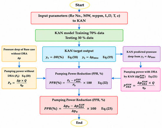
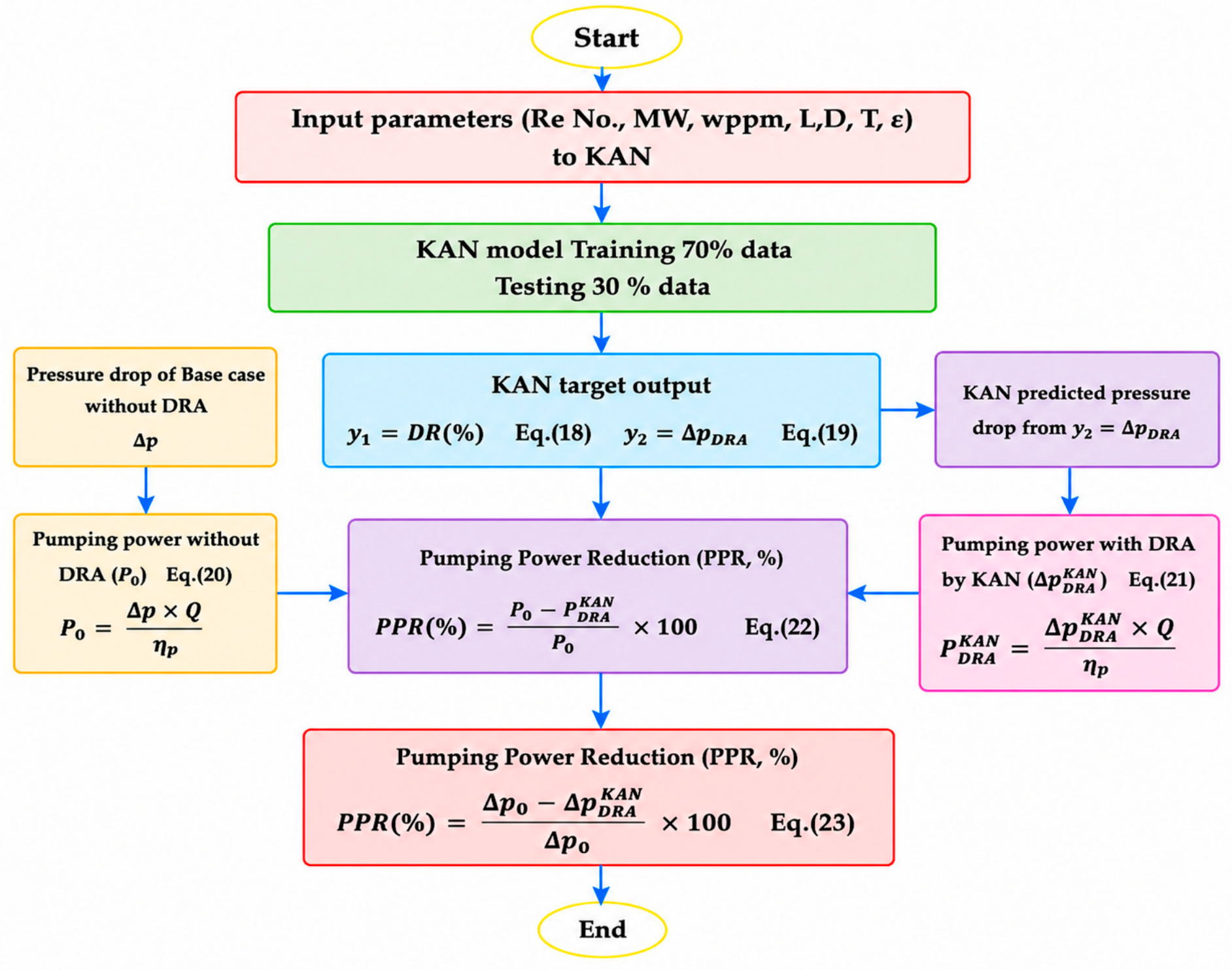
The Kolmogorov–Arnold Network (KAN) model is a neural network (NN) architecture based on the Kolmogorov–Arnold representation theorem, where learnable activation functions replace fixed weights. Figure 2 shows the detailed steps involved from input to target output.

Figure 2. Flowchart for pumping power reduction (PPR) based on the KAN regression model.

The KAN model is trained on the regenerated data by using one or more target outputs. The flowchart in Figure 2 explains the detailed steps, and the equations are given below:

$$y_1=DR\left(\%\right)$$

(18)

$${ y}_2=\Delta p_{DRA}$$

(19)

where $y_1$ is the target output 1 (DR); and $y_2$ is the target output 2, ($\Delta p_{DRA}$).

For energy analysis, pumping power can be calculated from Equations (20) and (21) as below:

$$P_0={\displaystyle \frac{{\Delta p}_0\times Q}{{\mathsf{\eta }}_p}}$$

(20)

$$P_{DRA}^{\mathrm{KAN}}={\displaystyle \frac{\Delta p_{DRA,i}^{\mathrm{KAN}}\times Q}{{\mathsf{\eta }}_p}}$$

(21)

where $P_0$ is the pumping power without DRA, (Watt); $P_{DRA}^{\mathrm{KAN}}$ is the pumping power with DRA predicted by KAN, (Watt); ${\Delta p}_0$ is the pressure drop without DRA, (Pa); $\Delta p_{DRA,i}^{\mathrm{KAN}}$ is the pressure drop with DRA, (Pa); $Q$ is the flow rate, (${\displaystyle \frac{\mathrm{L}}{\mathrm{h}}}$); and ${\mathsf{\eta }}_p$ is the pumping efficiency, (%). The pumping power saving can be calculated by Equation (22) as follows:

$$\% Pumping Power Reduction (W) ={\displaystyle \frac{P_0-P_{DRA}}{P_0}} \times 100$$

(22)

Pumping power reduction (W) by using the pressure drop is given as follows:

$$\% Pumpinp Power Reduction (W) = {\displaystyle \frac{{\Delta p}_0-\Delta p_{DRA,i}^{\mathrm{KAN}}}{{\Delta p}_0}} \times 100$$

(23)

3.4.3. KAN Mathematical Architecture

The mathematical architecture in terms of input features (X) and output target variables (y) can be written as in Equation (24):

$$\widehat{y}=KAN\left(X\right)$$

(24)

For only one input layer, it is given as in Equation (25):

$$x_j^{\left(l+1\right)}=\sum _{i=1}^{n_l}{\varphi }_{ij}^{\left(l\right)}\left(x_i^{\left(l\right)}\right)$$

(25)

where ${\mathsf{\varphi }}_{ij}^{\left(l\right)}\left(x\right)$ represents the learnable spline function between input node i and output node j.

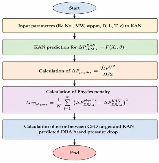
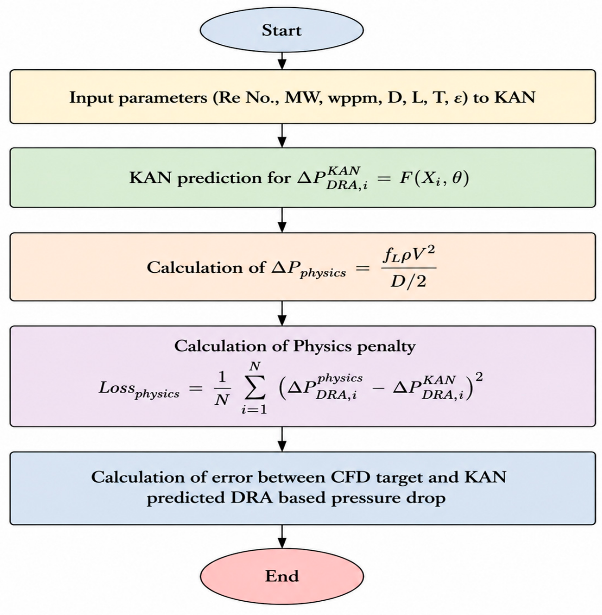
$\Delta P_{DRA,i}^{\mathrm{physics}}$ is the physics-based DRA reference term, which is calculated analytically by using the Darcy–Weisbach equation during the training process. For every training iteration, the predicted pressure drop from the KAN model is compared with the pressure-drop reduction calculated from the Darcy–Weisbach relationship incorporating the polymer-induced friction factor modification. The calculation procedure for Equation (26) is given below in sequential order.

The detailed steps involved in the fundamental understanding of Equation (26) are given in Figure 3, which represents the proposed physics-informed loss function based on the drag-reduction assessment (DRA), which consists of two terms as given below:

$$Loss={\displaystyle \frac{1}{N}}\sum _{i=1}^N{\left(y_i-\widehat{y_i}\right)}^2+\mathsf{\lambda }{\displaystyle \frac{1}{N}}\sum _{i=1}^N{\left(\Delta P_{DRA,i}^{\mathrm{physics}}-\Delta P_{DRA,i}^{\mathrm{KAN}}\right)}^2$$

(26)

where $\mathsf{\lambda }$ is the coefficient that controls the strength of the physical constant; $y_i$ is the CFD-based target value; and $\widehat{y_i}$ is the KAN-predicted DRA values.

Figure 3. Flowchart for loss function calculation using KAN.

This term ensures that the developed model learns the nonlinear relationship between the input parameters and the observed drag-reduction behavior. The second term represents the physics-based penalty component, where $\Delta P_{DRA,i}^{\mathrm{physics}}$ is the physically calculated drag-reduction values; and $\Delta P_{DRA,i}^{\mathrm{KAN}}$ is the DRA predicted by the KAN model. The purpose of this term is to restrict the model predictions within the physically meaningful range and reduce deviations from the governing fluid-flow principles. Figure 3 shows the flowchart for loss function calculation by using KAN.

Equation (27) shows that the dataset is normalized using standard scaling as given below:

$$X_{\mathrm{scaled}}={\displaystyle \frac{X-{\mathsf{\mu }}_X}{{\mathsf{\sigma }}_X}}$$

(27)

where $X_{\mathrm{scaled}}$ is the scaled value; ${\mathsf{\mu }}_{\mathrm{X}}$ is the original data value; $X$ is the average of all x values; and ${\mathsf{\sigma }}_X$ is the standard deviation of x.

4. Methodology

The present study includes a CFD-KAN coupled methodology to validate and predict an experimental benchmark. Karami et al. (2012) [32] particularly included drag reduction (DR) and pumping power reduction (PPR) for crude-oil pipeline systems.

In this study, CFD-based simulations were performed using the SST k-ω 2-equation turbulence model to validate an experimental benchmark and to investigate the turbulent flow behavior of a drag-reducing agent (DRA) solution in crude oil. The DRA solution was treated as a non-Newtonian fluid, in comparison to crude oil as a Newtonian fluid, at high temperature, and a power-law model was adopted to describe its shear-thinning behavior, which is commonly observed in polymer solutions. This rheological representation is important because viscosity variation under shear strongly influences drag reduction (% DR), pressure drop (∆p), pumping power reduction (PPR), energy savings (ES), and overall flow dynamics.

The boundary conditions used in the simulations were selected according to the experimental operating conditions. A constant inlet velocity was specified at the pipe inlet, while a turbulence intensity of 10% was applied to represent turbulent inflow conditions. At the outlet, a pressure outlet boundary condition with zero-gauge pressure was imposed. A no-slip boundary condition was applied at the pipe wall, together with appropriate wall treatment to resolve the near-wall flow behavior. These boundary conditions were chosen to reproduce the realistic turbulent flow conditions associated with polymer drag reduction.

The assumptions employed for CFD modelling are given below:

• The fluid flow was assumed to be steady-state.
• The working fluid was considered incompressible, with negligible density variation during the simulations.
• The flow was assumed to be isothermal, and heat-transfer effects were negligible.
• No-slip conditions were imposed at the pipe wall.
• The pipe wall was treated as impermeable, with no mass transfer through the wall.
• The flow was considered fully developed turbulent flow over the investigated Reynolds number range.
• For multiphase cases, the phases were assumed to follow the selected continuum/multiphase formulations without explicitly resolving molecular-scale interfacial phenomena.
• Polymer degradation or mechanical chain scission due to turbulent eddies were not explicitly modeled.
• The inlet flow conditions were assumed to be uniform and stable for each simulation.
• The simulations assumed that the flow was primarily pressure-driven.
• Gravity effects were neglected where their contribution to the axial pressure drop was insignificant.
• Numerical simulations were assumed to be sufficiently converged once the specified residual and solution-monitor convergence criteria were satisfied.

The details of further assumptions are given below in Table 1 and Table 2. For the numerical solution, the SIMPLE algorithm was employed for pressure–velocity coupling to ensure stable and accurate convergence. Second-order discretization schemes were applied to the momentum and turbulence transport equations in order to improve numerical accuracy and capture the flow gradients more effectively. These solver settings were selected to enhance the reliability of the CFD predictions for complex turbulent flow involving non-Newtonian polymer solutions. Table 3 represents the turbulence models with features.

Table 1. CFD simulation setup and numerical simulations used in ANSYS Fluent 24 academic version using an experimental benchmark [32].

Category	Parameter	Specification
Working fluid properties	Base fluid	Crude oil
	Working fluid	Crude-oil-based drag-reducing polymer solution
	Fluid type	Newtonian (base); non-Newtonian (DRAs)
	Boiling temperature	DRA1 (163.2 °C); DRA2 (150.8 °C); DRA3 (147.3 °C); Crude oil (50 °C)
	Rheological model	Power-law model for DRA polymer solution
	DRAs concentration	25; 75; 100; 150; 200 wppm
Geometry and computational domain	Flow configuration	Internal pipe flow
	Pipe 1 diameter (D)	0.0254 m
	Pipe 2 diameter (D)	0.0254 m
	Pipe 3 diameter (D)	0.0127 m
	All Pipe length (L)	8 m
	Fluid domain	Single continuous fluid region
	Fluid–fluid boundary conversion	Wall boundaries maintained and not converted into internal interfaces
	Share topology	Disabled
	Multizone meshing	Disabled
Flow conditions	Flow regime	Turbulent internal pipe flow
	Reynolds number	6104.88–16,777.77
	Flow assumption	Incompressible steady-state flow
Inlet boundary conditions	Boundary type	Inlet velocity
	Turbulence intensity	10%
	Hydraulic diameter	0.0254 m; 0.0127 m
	Turbulence length scale	Hydraulic diameter-based estimation
Outlet boundary conditions	Boundary type	Pressure outlet
	Gauge pressure	zero
	Pressure profile multiplier	1
	Backflow turbulence viscosity ratio
Wall boundary conditions	Wall assumption	Stationary no-slip wall
	Wall roughness	Smooth wall assumptions
	Energy transfer	Adiabatic conditions
	Phase definition	Mixture phase (water and DRAs)
Multiphase model	Multiphase approach	Volume of fluid (VOF)

Table 2. CFD simulation and numerical parameters used in current study using ANSYS Fluent 24 academic version.

Category	Parameter	Specification
Mesh generation	Meshing software	ANSYS Fluent Meshing
	Mesh type	Polyhedral volume mesh
	Surface mesh methods	Curvature and proximity-based sizing
	Smallest unit dimension	0.001953 m
	Maximum surface element size	0.05 m
	Surface cell generation rate	1.2
	Bend theta	1
	Proximity analysis	Edges
	Boundary separation	Disabled
Boundary layer mesh	Boundary layer generation	Enabled
	Boundary layer method	Smooth transition
	Quantity of layers	3
	TR	0.272
	Boundary generation rate	1.2
	Applied region	Fluid region
	Growth surfaces	Wall surfaces only
Solver settings	CFD software	ANSYS fluent
	Solver type	Pressure-based solver
	Velocity formulation	Absolute velocity
	Time formulation	Steady-state
	Gravity	Neglected
Turbulence models	Turbulence model	SST (2-equation)
	Near-wall treatment	Enhanced wall treatment
Initialization	Initialization method	Hybrid initialization
	Initial velocity field	Based on inlet velocity
	Initial turbulence quantities	Automatically calculated
Convergence criteria	Continuity residual	<10−3
	Momentum residual	<10−3
	Turbulence residual	<10−3
	Monitoring parameters	Friction factor (ƒ), drag reduction (DR), pumping power reduction (PPR), and energy savings (ES)
Output parameters	Friction factor (ƒ)	Obtained from inlet–outlet pressure difference
	Drag reduction (DR)	Calculated relative to water case
	Pumping power reduction (PPR)	Calculated from pressure drop and flow rate
	Energy savings (ES)	Evaluated based on the reduction in PP compared with water case

Table 3. Reynolds-average Navier–Stokes model section [32,33,34,35].

Model	Description
Spalart–Allmaras	A model with a single transport equation that solves directly for a modified turbulent viscosity. It converges at medium to high iterations. Medium CPU and memory requirements. Not suitable for turbulent dissipation rate and kinetic energy.
Standard k-ε	A model with two transport equations solving for turbulent production rate (k) and dissipation rate (ε). This is also called the default k-ε model. Coefficients are empirically derived. It is used only for turbulent flows. It takes time to converge. High CPU and memory requirements.
RNG k-ε	A variant of the standard k-ε model. Variables and equations are analytically derived.
Realizable k-ε	This variant of the standard k-ε model improves its realizability by incorporating modifications that ensure the specific mathematical constraints are satisfied. It is easier and more accurate than the RNG k-ε model.
Standard k-ω	A model with two transport equations solving for k and ω, the specific dissipation rate (${\displaystyle \frac{\epsilon }{k}}$) based on Wilcox (1998) [28]. It is also called the default k-ω model. It takes time to converge at low to high iterations.
SST k-ω (Present study)	Modified form of the standard k-ω model. It integrates the original Wilcox model closer to the wall and the standard k-ε model away from the wall by using a blending function. Best for turbulent dissipation rate and production of turbulent kinetic energy reduction. Convergence is easy at low iterations. Medium CPU and memory requirements (i.e., RAM 32 GB and processor 32 GB)
Reynolds Stresses	Physically the most applicable RANS model. It does not include the isotropic eddy viscosity assumption. It takes too much time to converge due to the close coupling of equations. High-resolution CPU and memory requirements (i.e., more than 128 GB RAM and processor). Best for complex 3D turbulent flows.

To avoid overfitting and data leakage, the datasets for the KAN model were constructed using an original experimental benchmark incorporating crude-oil flow with DRAs under varied operational conditions. In addition, all normalization and scaling parameters were calculated exclusively from the training data and were not estimated using validation or external test observations. The external test results were evaluated only after completion of the model-development process, thereby preventing information from the test dataset from influencing the trained model. Duplicate observations and identical operating conditions records were also checked to ensure that the same data points were not included simultaneously in the training and external-test datasets.

The KAN modelling assumptions adopted are given below:

• The selected input variables were assumed to contain the dominant information required to predict the target response.
• The available experimental and CFD dataset was assumed to be representative of the investigated operating conditions.
• The relationships between the input variables and output response were assumed to be continuous and learnable by the KAN model.
• The training and testing datasets were assumed to originate from the same underlying physical system and parameter domain.
• The KAN predictions were assumed to be reliable mainly within the range of input variables used for model development.
• Extrapolation outside the investigated input range was not assumed to be reliable and was therefore not considered in evaluating model performance.
• The input data were assumed to be sufficiently accurate, with no significant systematic experimental or CFD bias affecting the learnable relationships.
• The selected KAN architecture and hyperparameters were assumed to provide sufficient flexibility to capture nonlinear input–output relationships without excessive overfitting.
• The independent test dataset and 5-fold cross-validation were assumed to provide a suitable assessment of the model’s generalization capacity and prediction stability.
• The predictive uncertainty of the KAN model was assumed to be adequately represented by the independent test-set error metrics, particularly R², RMSE, MAE, and MSE, rather than by training performance alone.

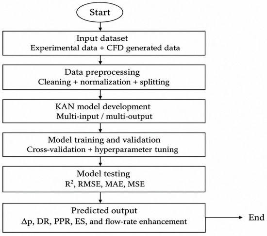
Figure 4 shows the KAN framework involving inputs and target output variables. The KAN workflow uses the combined experimental–CFD-generated dataset, followed by preprocessing, multi-input and output model development, cross-validation, and hyperparameter tuning. Model performance is evaluated using R², RMSE, MAE, and MSE, and the trained KAN predicts ∆p, DR, PPR, ES, and flow-rate enhancement.

Figure 4. KAN framework for the current study.

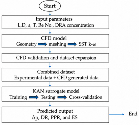
Figure 5 presents the CFD-KAN integrated framework. The proposed framework integrates CFD simulations with experimental data to generate and validate an expanded dataset using key pipeline and DRA operating parameters. The combined dataset is then used to train, test, and cross-validate the KAN surrogate model for predicting pressure drop (∆p), drag reduction (DR), pumping power reduction (PPR), and energy savings (ES).

Figure 5. Integrated CFD-KAN framework.

A total of N = 1000 samples were generated from an experimental benchmark by defining the minimum and maximum values of the experimental input parameters (i.e., Re No., polymer ppm, input velocity, etc.). Latin Hypercube sampling (LHS) is then used to produce well-distributed combinations of these input variables within the experimentally validated ranges. Each generated combination is introduced into a validated Volume of Fluid (VOF) model in ANSYS Fluent as a separate design point, and the corresponding outputs, such as ∆p, DR, PPR, and ES, are calculated. In this way, LHS combined with CFD expands the available datasets efficiently while maintaining physical consistency with the experimental conditions covering a wide range of Reynolds numbers (Re), DRA concentrations, and pipeline operating conditions. The dataset was randomly split into training (80%, 800 samples) and validation (20%, 200 samples) to ensure a robust model.

Overall, the independent test-set performance was used as the primary indication of the expected predicted error for previously unseen data within the investigated parameter range. The uncertainty associated with the CFD predictions arise from factors including mesh resolution, numerical convergence, turbulence, multiphase modelling assumptions, boundary conditions, and uncertainties in the input material and operating parameters. A mesh-independent assessment was performed to minimize the influence of spatial discretization on the reported CFD results. Figure 6 presents the steps involved in KAN model deployment.

Figure 6. Steps involved in KAN model deployment.

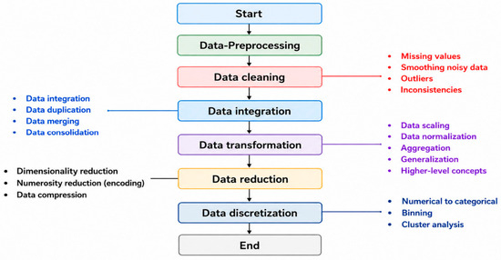
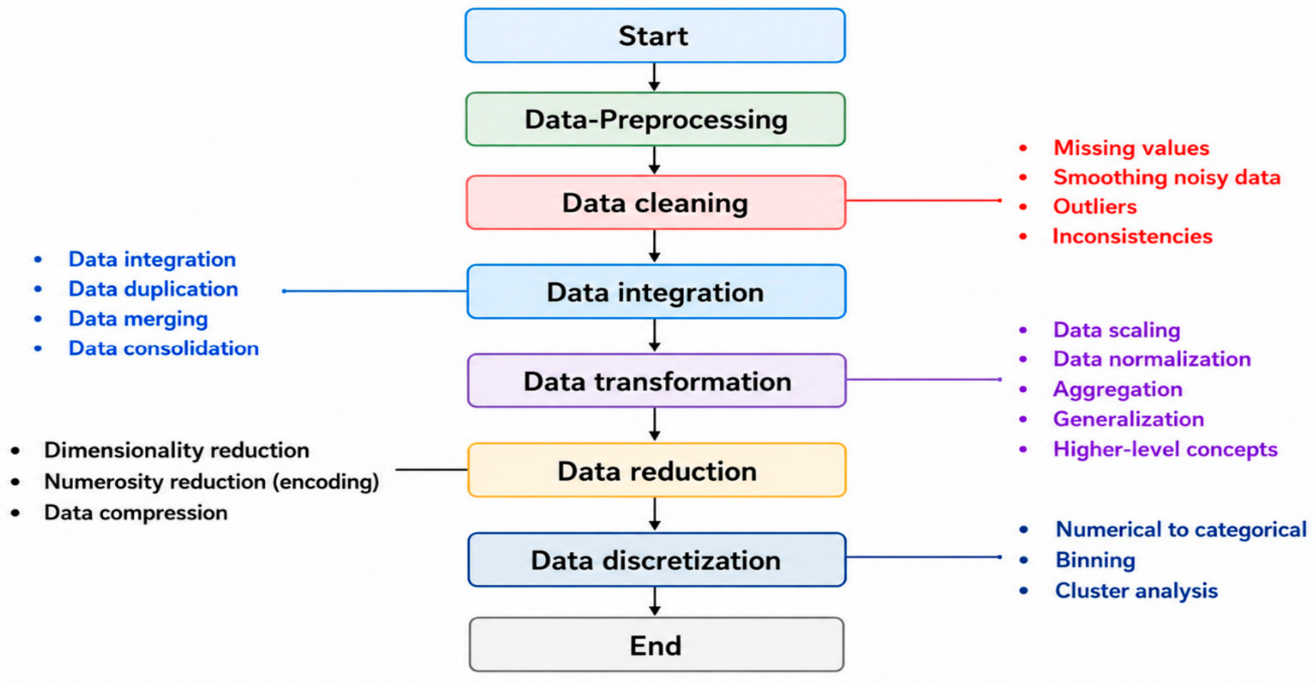
Figure 7 below indicates the steps involved in CFD generation data preprocessing.

Figure 7. Steps involved in CFD-generated data preprocessing.

Table 4 presents the mesh independence based on SST k-ω.

Table 4. Mesh independence table (SST k-ꞷ and polyhedral mesh).

Mesh Case	Number of Elements	Average Element Size (mm)	Mean y+	Max y+	∆p (Pa)	DR (%)	PPR (W)	Remarks
Mesh 1 (Coarse)	5.8 × 104	3.6	37	45	129.5	31.1	35	Initial coarse mesh. Provides a baseline for comparing pressure drop (∆p), drag reduction (DR), and pumping power reduction (PPR)
Mesh 2	8.6 × 104	2.9	33	40	130.50	31.40	35.30	Grid refinement improves the near-wall resolution and reduces the difference from the fine-grid solution
Mesh 3	1.6 × 105	2.3	26	34	131.50	31.65	35.55	∆p, DR, and PPR begin to stabilize, although the near-wall resolution remains insufficient
Mesh 4	2.5 × 105	1.9	5.5	31	132.50	31.85	35.80	Strong stabilization is observed. The variations relative to Mesh 5 are below 1% for all monitored quantities (∆p, DR, and PPR)
Mesh 5 (Fine)	3.8 × 105	1.5	0.55	1	133.1	32	36	Mesh independence confirmed. It provides adequate wall-resolved conditions and the lowest numerical uncertainty. It is selected as the final computational mesh

Table 5 shows the Grid convergence index (GCI) and estimated numerical accuracy.

Table 5. Grid convergence index (GCI) and estimated numerical uncertainty.

Quantity	Coarse Value, Mesh 3	Medium Value, Mesh 4	Fine Value, Mesh 5	Refinement Ratio, r21	Assumed Order, p	Fine-Grid GCI (%)	Estimated Numerical Uncertainty	Remarks
Pressure drops (∆p)	131.50	132.50	133.10	1.267	2.0	0.93	±1.24 Pa	Acceptable pressure-drop uncertainty; fine mesh retained
Drag reduction (DR %)	31.65	31.85	32	1.267	2.0	0.97	±0.31%	Acceptable monotonic convergence with low residual mesh uncertainty
Pumping Power Reduction (PPR)	35.55	35.80	36.00	1.267	2.0	1.15	±0.41 W	Acceptable monotonic convergence with GCI below 3%

Table 6 presents the mesh sensitivity analysis based on the critical parameters.

Table 6. Mesh sensitivity analysis.

Mesh Case	∆p (Pa)	∆p Deviation from Mesh 5 (%)	DR (%)	DR Deviation from Mesh 5 (%)	PPR (W)	PPR Deviation from Mesh 5 (%)	Mesh Sensitivity Assessments
Mesh 1 (coarse)	129.50	2.70	31.10	2.81	35	2.78	All monitored global quantities remain within the prescribed 3% limit, although near-wall resolution is inadequate
Mesh 2	130.50	1.95	31.40	1.88	35.30	1.94	Mesh sensitivity is reduced with deviation below 2%
Mesh 3	131.50	1.20	31.65	1.09	35.55	1.25	The monitored quantities approach the fine-grid solution, with deviation close to 1%
Mesh 4	132.50-	0.45	31.85	0.47	35.80	0.56	The solution is nearly stabilized, with all deviations below 1%
Mesh 5 (Fine)	133.10	0.00	32.00	0.00	36.00	0.00	Final reference mesh providing adequate wall resolution and acceptable uncertainty

Table 7 illustrates the features of turbulence model employed in the current study.

Table 7. Selected turbulence model SST k-ω.

Model	Fundamental Principle	Near-Wall Approach	Strength	Weakness	Multiphase Use	Numerical Stability	Remarks
SST k-ω	Combines the k-ω model near the walls with the k-ε model in the free-stream, creating a hybrid approach for improved accuracy	Captures the viscous sublayer behavior directly without relying on wall functions	Provides reliable predictions for wall shear stress, flow separation, and turbulence control	Requires slightly more computational resources compared to standard models	Compatible with Volume of Fluid (VOF) and Eulerian multiphase modeling techniques	Well-suited for simulations involving polymer-induced drag reduction	Outperforms the conventional k-ε and k-ω models near-wall turbulence scenarios

Table 8 and Table 9 presents the comparison of the results based on experimental and present work.

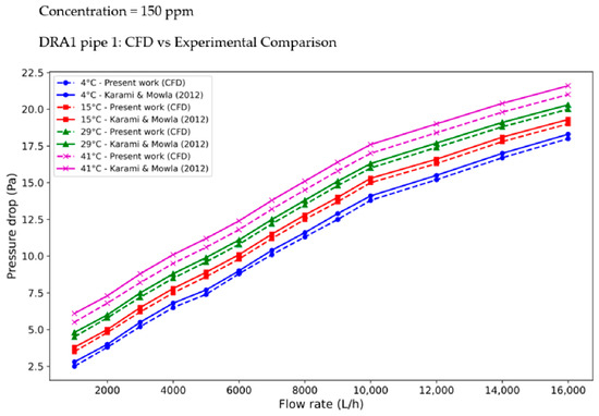
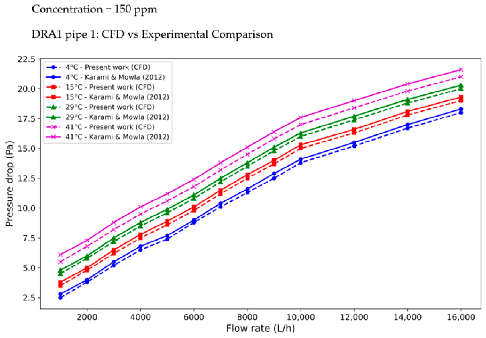
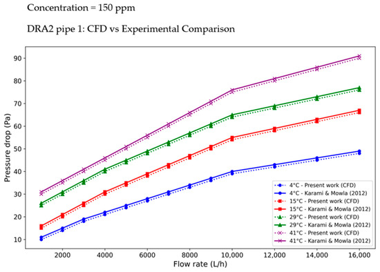
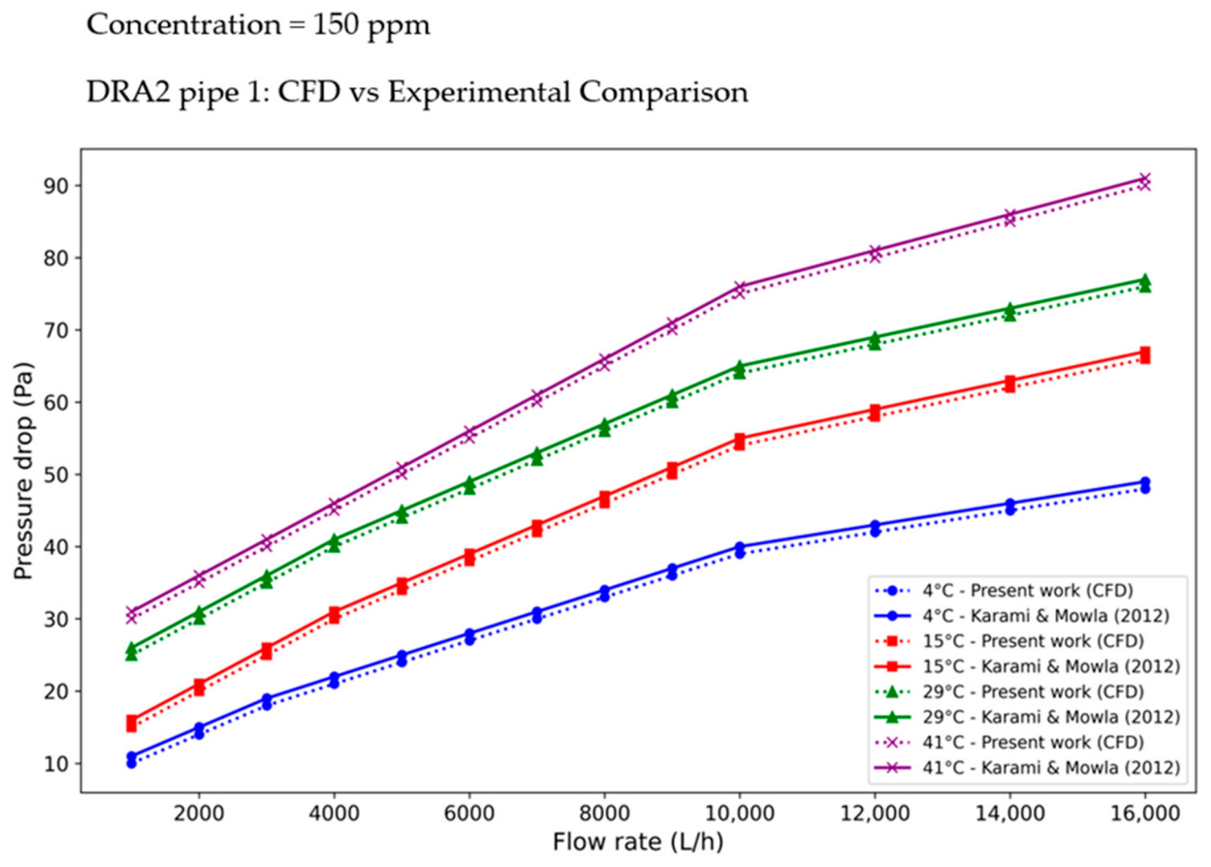
Table 8. Comparison of the results of the present study with those of Karami & Mowla’s (2012) [32] experimental pressure drop (Pa) without DRA.

Q ($\frac{\mathbf{l}}{\mathbf{h}}$)	Reynolds No. (Re)	Experimental [32]	Present Study
		∆p (Pa)	${∆\mathit{p}}_{\mathit{p}\mathit{r}\mathit{e}\mathit{s}\mathit{e}\mathit{n}\mathit{t}\mathit{s}\mathit{t}\mathit{u}\mathit{d}\mathit{y}}$ (Pa)	DR (%)
1775	6104.84	2775.1	2500.9	9.8
2620	9940.11	5213.4	5103.6	2.1
3352	13,535.89	7698.3	7580	1.5
3980	16,777.77	10,262.	10,000	2.5

Table 9. Comparison of the results of the present study with those of Karami & Mowla’s (2012) [32] experimental pressure drop (Pa) with DRA.

Re	C (ppm)	Experimental [32]		Present Study
		∆p (Pa)	DR (%)	${∆\mathit{p}}_{\mathit{P}\mathit{r}\mathit{e}\mathit{s}\mathit{e}\mathit{n}\mathit{t}\mathit{s}\mathit{t}\mathit{u}\mathit{d}\mathit{y}}$ (Pa)	${\mathit{D}\mathit{R}}_{\mathit{p}\mathit{r}\mathit{e}\mathit{s}\mathit{e}\mathit{n}\mathit{t}\mathit{s}\mathit{t}\mathit{u}\mathit{d}\mathit{y}}$ (%)	% Error
6104.84	25	2687.6	3.2	2620.1	5.5	2.5
9940.11	25	4993.9	4.2	4910.3	5.8	1.6
13,535.89	25	7314.9	4.9	7290.1	5.3	0.3
16,777.77	25	9652.1	5.9	9612.5	6.3	0.4
6104.84	50	2669.3	3.8	2613.4	5.8	2.0
9940.11	50	4950.6	5.0	4948.5	5.0	0.1
13,535.89	50	7153.2	7.1	7099.3	7.7	0.7
16,777.77	50	9260.1	9.8	9248.2	9.8	0.1
6104.84	75	2587.5	6.8	2579.6	7.0	0.3
9940.11	75	4742.1	9.0	4712.5	9.6	0.6
13,535.89	75	6776.1	11.9	6773.1	12.0	0.04
16,777.77	75	8731.5	14.9	8712.6	15.1	0.2
6104.84	100	2363.4	14.8	2343.7	15.5	0.8
9940.11	100	4222.2	19.01	4128.5	20.8	2.2
13,535.89	100	6019.9	21.8	6012.8	21.8	0.1
16,777.77	100	7679.4	25.17	7700.2	25.0	0.2
6104.84	150	2084.9	24.87	2078.3	25.1	0.3
9940.11	150	3569.6	31.53	3520.9	32.2	1.3
13,535.89	150	5079.3	34.02	5048.8	34.4	0.6
16,777.77	150	6296.2	38.65	6290.4	38.7	0.1
6104.84	200	2017.7	27.29	2012.8	27.4	0.2
9940.11	200	3405.9	34.67	3400.3	34.7	0.1
13,535.89	200	4755.6	38.22	4700.4	38.9	1.1
16,777.77	200	5741.1	44.06	5721.2	44.2	0.3

5. Results and Discussion

5.1. Five-Fold Cross-Validation

A 5-fold robustness analysis was subsequently performed on the independent external dataset. The experimental observations were divided into five subsets containing 5,5,5, and 4 observations. Model performance was assessed separately within each fold using coefficient of determination (R²), mean squared error (MSE), root mean squared error (RMSE), and mean squared error (MSE). From the five machine learning models (ML), KAN outperforms the prediction with the highest coefficient of determination (R² = 0.9753 and 0.9687), lower mean squared error for DR (%) and PPR (MSE = 3.1512 and 4.2353), lower root mean squared error (RMSE = 1.7751, 2.0580), and lower mean absolute error (MAE = 1.3082 and 1.5669). The results were subsequently expressed as the mean ± standard deviation across the five folds, as given below in Table 10 for drag reduction and in Table 11 for pumping power reduction.

Table 10. 5-fold cross-validation based on DR (%).

Fold	Model	Mean R2 ± Std	Mean MSE ± Std	Mean RMSE ± Std	Mean MAE ± Std
Fold 1	KAN	0.9687 ± 0.0019	4.2353 ± 0.0355	2.0580 ± 0.0086	1.5669 ± 0.0429
Fold 2	ANN	0.9543 ± 0.0021	5.5920 ± 0.1748	2.3645 ± 0.0370	1.8820 ± 0.0526
Fold 3	NAN	0.9607 ± 0.0020	4.9980 ± 0.1366	2.2355 ± 0.0306	1.7620 ± 0.0460
Fold 4	GBR	0.9637 ± 0.0018	4.7500 ± 0.1420	2.1793 ± 0.0326	1.6880 ± 0.0415
Fold 5	SVR	0.9494 ± 0.0020	6.1120 ± 0.1794	2.4720 ± 0.03630	2.0060 ± 0.0573

Table 11. 5-fold cross-validation based on pumping power reduction (PPR).

Fold	Model	Mean R2 ± Std	Mean MSE ± Std	Mean RMSE ± Std	Mean MAE ± Std
Fold 1	KAN	0.9753 ± 0.0022	3.1512 ± 0.0560	1.7751 ± 0.0158	1.3082 ± 0.0562
Fold 2	ANN	0.9628 ± 0.0024	3.8210 ± 0.0912	2.0600 ± 0.0277	1.5400 ± 0.0430
Fold 3	NAN	0.9689 ± 0.0020	3.7500 ± 0.0828	1.9364 ± 0.0214	1.4280 ± 0.0349
Fold 4	GBR	0.9708 ± 0.0019	3.4680 ± 0.0907	1.8621 ± 0.0243	1.3880 ± 0.0349
Fold 5	SVR	0.9581 ± 0.0022	4.7000 ± 0.1000	2.1678 ± 0.0230	1.6400 ± 0.0430

5.2. Network Architecture for ANN, KAN, and NAN Models

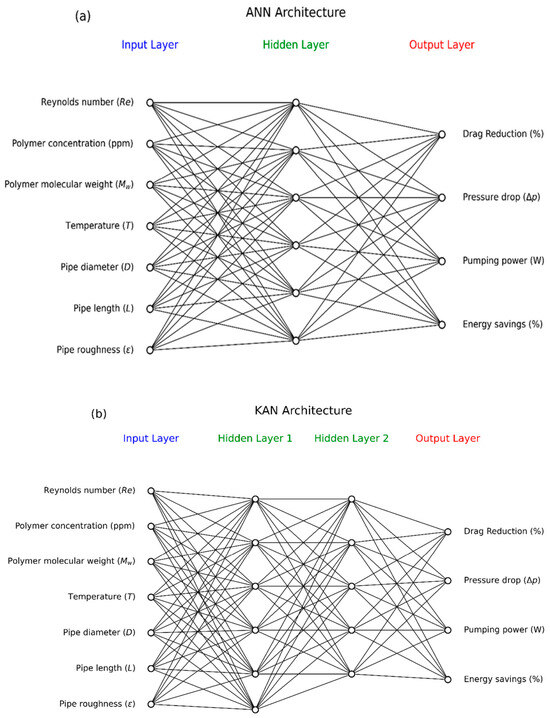
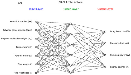
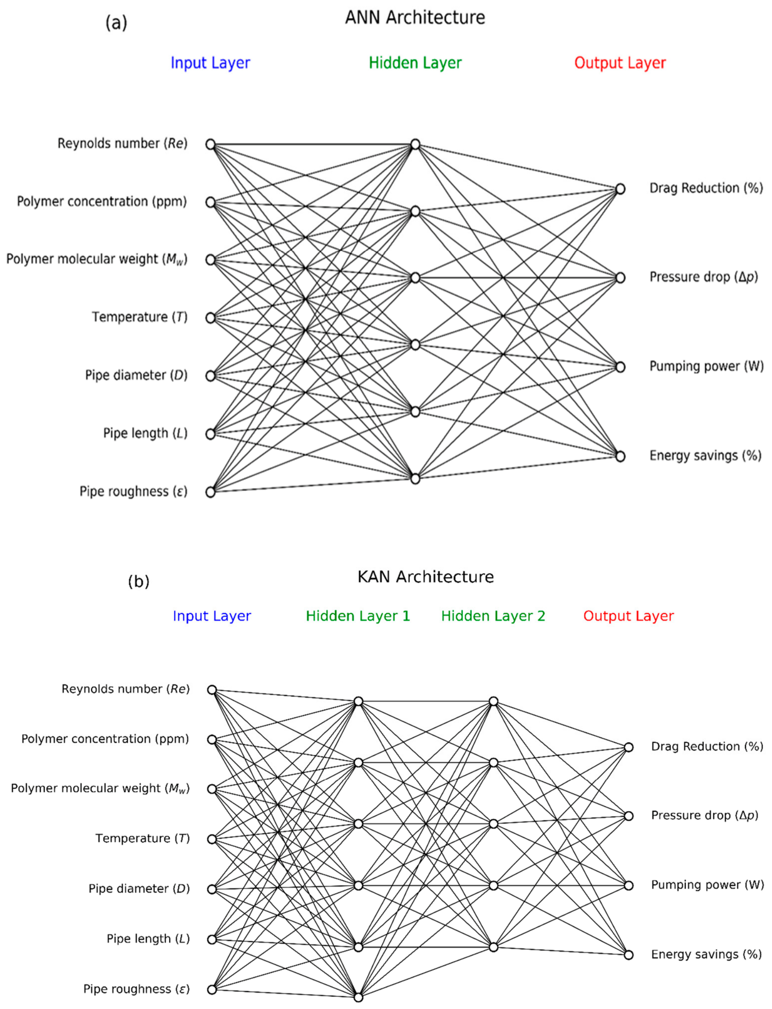
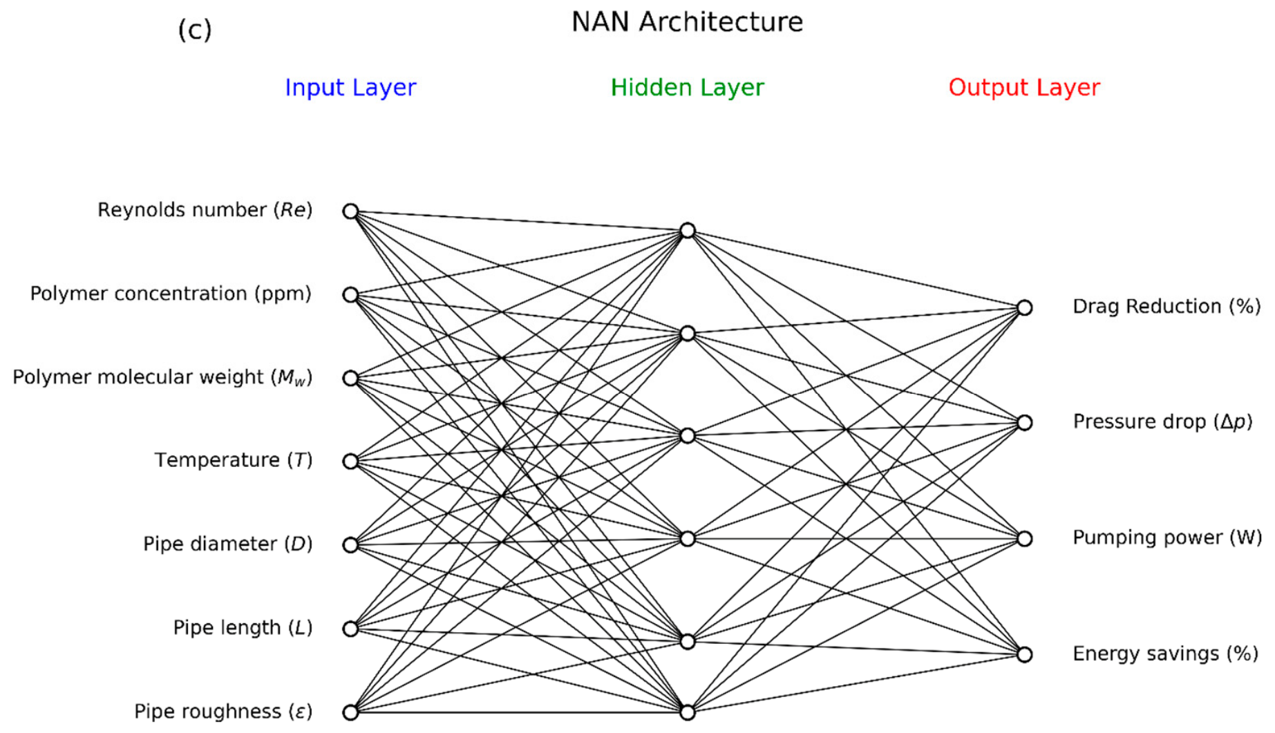
Figure 8 presents a comparison of the comprehensive architectures using an Artificial Neural Network (ANN), a Kolmogorov–Arnold Network (KAN), and an Adaptive Neural Network (NAN). ANN consists of one input layer (7 neurons), one hidden layer (5 neurons) and one output layer (4 neurons), KAN consists of one input layer (7 neurons), two hidden layers (11 neurons) and one output layer (4 neurons), and NAN consists of one input layer (7 neurons), one hidden layer (5 neurons) and one output layer (4 neurons). KAN, with two hidden layers of 11 neurons, provides the highest nonlinear modeling capacity among the neural networks considered, effectively capturing complex interactions in the dataset. It dominates the neural approaches for depth learning ability.

Figure 8. Comparison of the architecture structure with input, hidden, and output layers: (a) ANN; (b) KAN; (c) NAN.

5.2.1. Kolmogorov–Arnold Network (KAN)

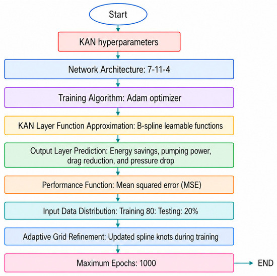
KAN consists of an input layer with 7 nodes representing the Reynolds number (Re), polymer concentration (ppm), polymer molecular weight (Mw), temperature (°C), pipe diameter (D), pipe length (L), and pipe roughness (ε), plus two hidden layers with 11 neurons and an output layer with 4 neurons corresponding to drag reduction (% DR), pressure drop (∆p), pumping power reduction (PPR), and energy savings (ES). All inter-layer connections employed B-spline functions to model smooth nonlinear transformations of inputs. To prevent overfitting, L2 regularization with a coefficient of ʎ = 0.01 was applied to all spline coefficients. The network was trained using an Adam optimizer, a learning rate of 0.001, and early stopping based on validation loss, with the dataset split into 80% training and 20% validation. This detailed description ensures that the KAN model is fully reproducible and aligns with the diagram provided.

5.2.2. KAN Hyperparameter Optimization

Figure 9 illustrates the KAN hyperparameter optimization procedure used for model training and predictions. The KAN network is configured with a 7-11-4 architecture consisting of 7 input neurons, 11 hidden neurons, and 4 output neurons. The model uses the Adam optimizer learnable B-spline functions training–testing splits; and a 1000 epochs to predict energy savings, pumping power, drag reduction, and pressure drop. Performance: The performance function is given as mean squared error.

Figure 9. KAN hyperparameter optimization procedure.

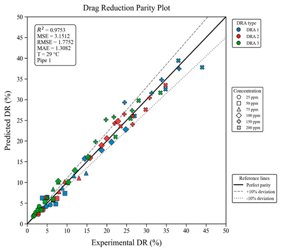
Figure 10 presents the parity plot for drag reduction (DR) at various concentrations (25 ppm–200 ppm). The model explained 97.53% variance in DR (R² = 0.9753) across three DRA types (DRA1, DR2, and DR3) and concentrations of 25–200 ppm at 29 °C in pipe 1. Prediction errors remained low, with MSE = 3.1512, RMSE = 1.7752, and MAE = 1.3082. Most predictions fell within the ±10% deviation bounds. The slight underpredictions at higher DR values, due to the limited number of higher DR observations, weaken its ability to capture nonlinear saturation behavior in extreme drag-reduction conditions.

Figure 10. Drag-reduction parity plot at various DRAs (DRA 1, 2, and 3) and various concentrations (25–200 ppm).

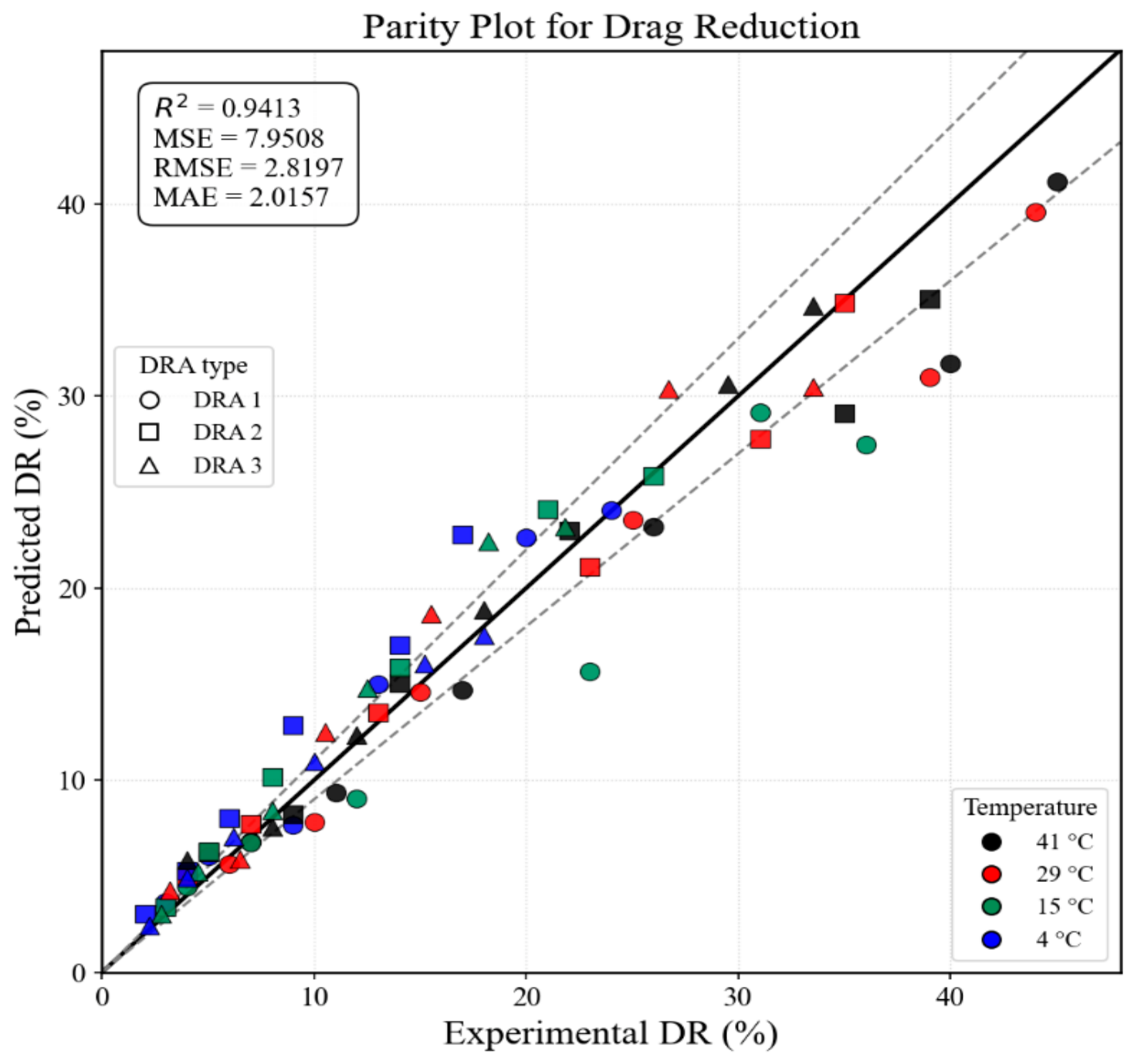
Figure 11 presents the parity plot for DR at various temperatures (i.e., 4, 15, 29, and 41 °C). The model exhibited good predictive accuracy across three DRAs and temperatures 4–41 °C, explaining 94.13% of the variance in DR (R² = 0.9413). The predicted errors remained moderate, with MSE = 7.9508, RMSE = 2.1897, and MAE = 2.0157, while most observations were confined within the deviation lines. A minor deviation reflects sparse high DRA data and stronger nonlinear temperature DRA interactions near the drag-reduction saturation regimes.

Figure 11. Parity plot for drag reduction (DR %) at various temperatures (i.e., 4, 15, 29, and 41 °C) at various drag-reducing agents (i.e., DRA 1, DRA 2, and DRA 3).

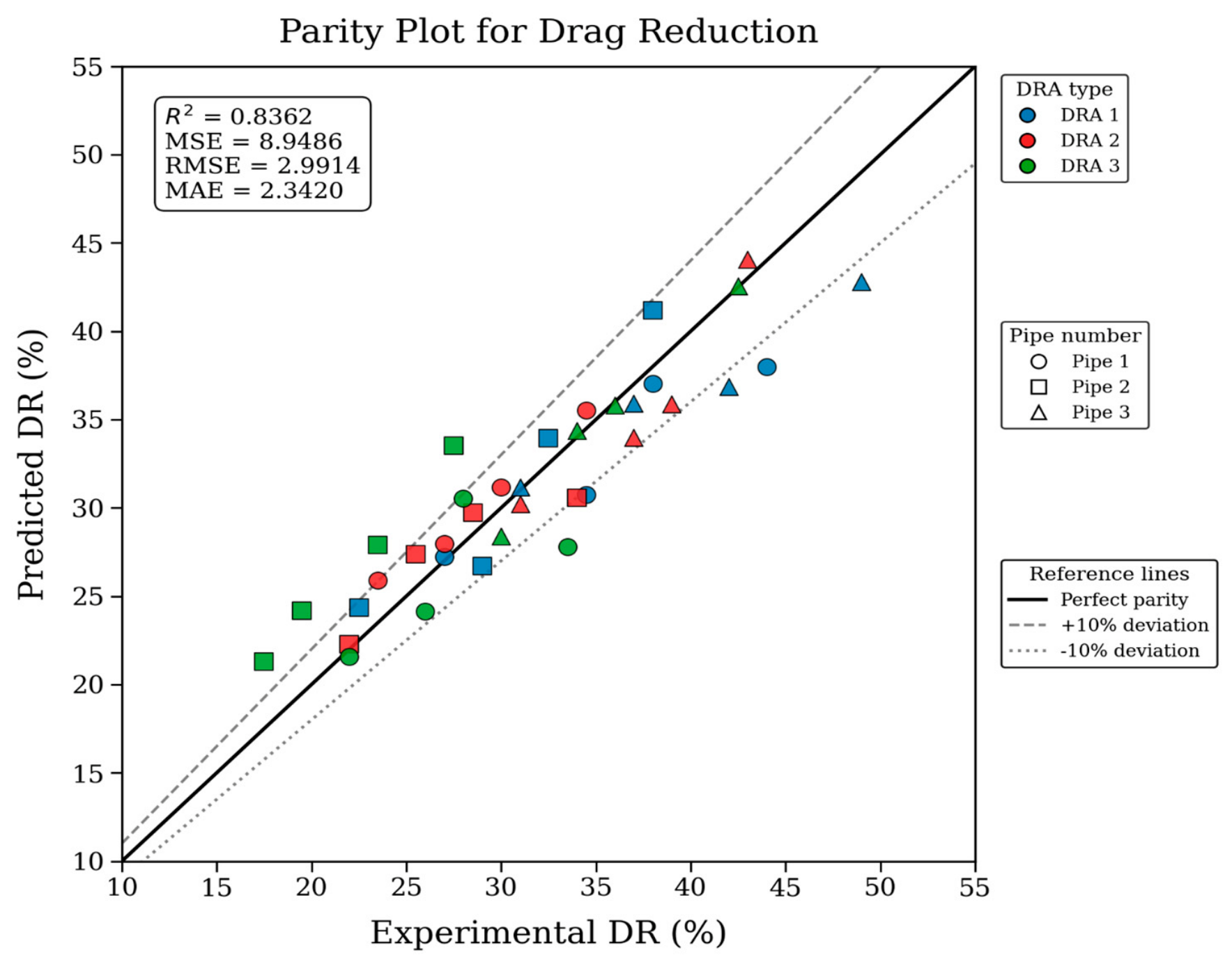
Figure 12 depicts the parity plot for drag reduction (DR) across the three different pipes at constant temperature (i.e., 29 °C). The model captured 83.62% of the DR variance (R² = 0.8362), with MSE = 8.9486, RMSE = 2.9914, and MAE = 2.3420, although some high-DR observations approached or exceeded the ±10% deviation limits. The maximum deviation is primarily attributed to pipe-dependent hydrodynamic heterogeneity, because changes in diameter, wall roughness, and Reynolds number alter wall shear stress, turbulent structures, and DRA–turbulence interactions. At higher DR, nonlinear saturation and possible shear-induced degradation of the drag-reducing molecules further weaken model extrapolation, producing the observed underprediction for data in pipe 3.

Figure 12. Parity plot for drag reduction (DR %) at three different pipes (Pipe 1, Pipe 2, and Pipe 3) and constant temperature (29 °C).

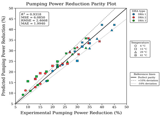
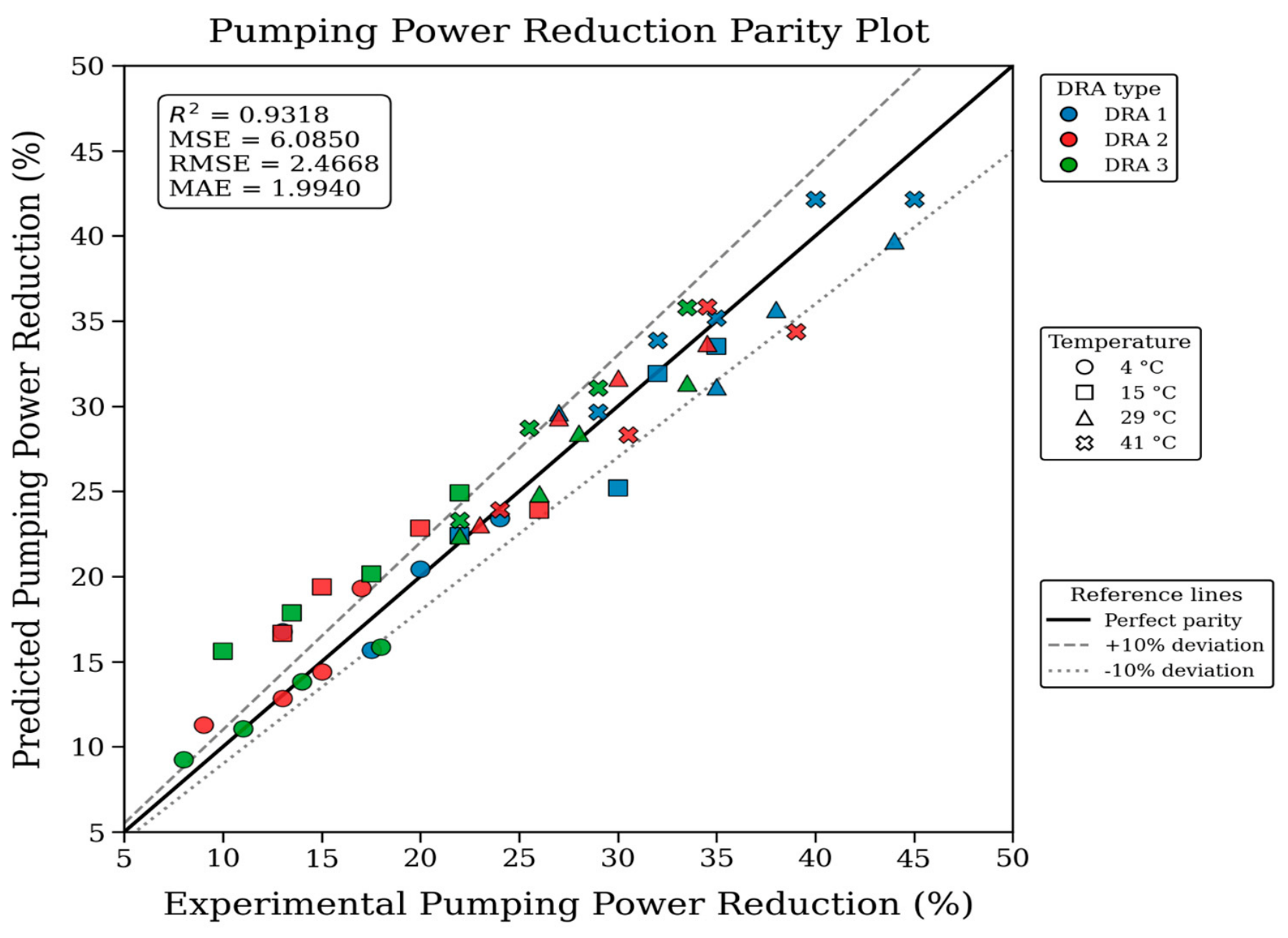
Figure 13 shows the parity plot for pumping power reduction (PPR) with different DRAs and temperatures (4 °C; 15 °C; 29 °C; 41 °C). The parity analysis demonstrates good agreement between experimental and predicted PPR across three different DRA types and temperatures (4–41 °C), yielding R² = 0.9318; MSE = 6.0850; RMSE = 2.4668; MAE = 1.9940, with most observations remaining within the acceptable deviation bounds. The observed variations are attributed to the compound’s sensitivity of PPR to uncertainties in pressure drop and flow rate, coupled with temperature-induced variations in viscosity, wall shear stress, and polymer conformations, which intensify nonlinear polymer–turbulence interactions under high drag-reduction conditions.

Figure 13. Parity plot for pumping power reduction (PPR) at various temperatures (4 °C; 15 °C; 29 °C; 41 °C) and DRAs (DRA 1; DRA 2; DRA 3).

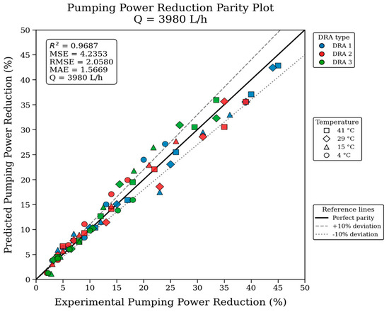
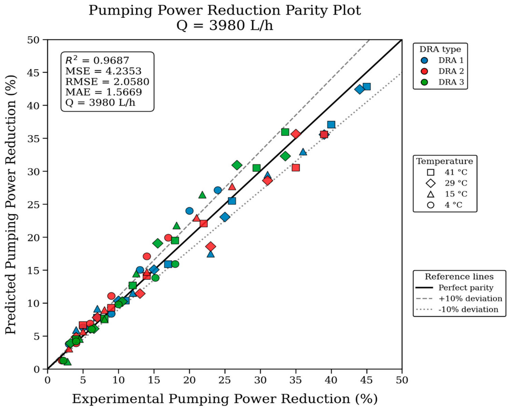
Figure 14 presents the parity plot for PPR at different temperatures (4 °C, 15 °C, 29 °C, and 41 °C) at a constant flow rate (Q = 3980 ${\displaystyle \frac{\mathrm{L}}{\mathrm{h}}}$). The model outperforms the experimental PPR across three different DRAs and temperatures (4–41 °C), achieving R² = 0.9687; MSE = 4.2353; RMSE = 2.0580; MAE = 1.5669. Most predictions remain within the ±10% deviations, confirming that the model captured the principal effect of DRA chemistry and temperature. The fluctuations are mainly attributed to temperature-driven changes in viscosity, velocity profile, polymer relaxation, etc., at the fixed flow rate.

Figure 14. Parity plot for pumping power reduction (PPR) at different temperatures (4 °C; 15 °C; 29 °C; 41 °C) at constant flow rate (Q = 3980 ${\displaystyle \frac{\mathrm{L}}{\mathrm{h}}}$).

5.3. Validation of Experimental Drag Reduction (DR %)

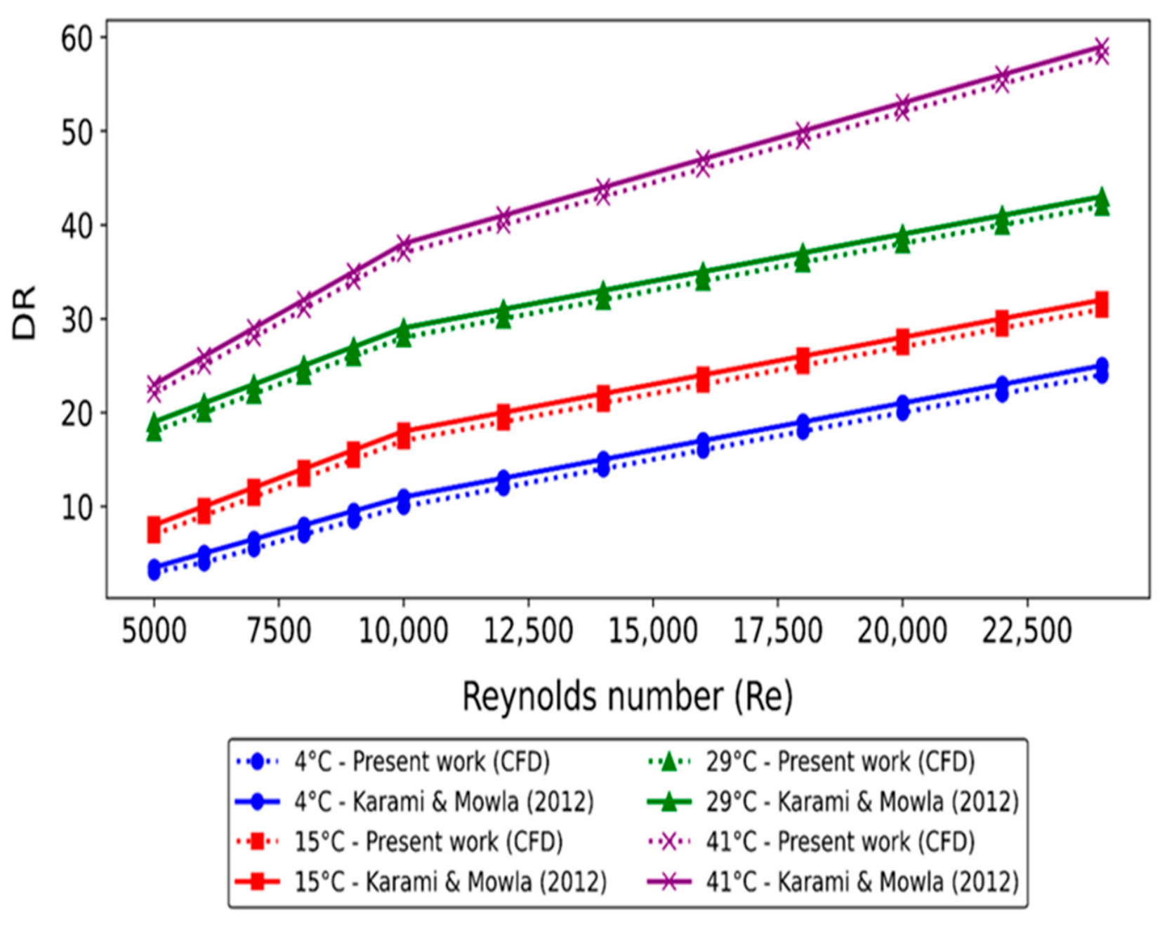
Figure 15 shows the CFD validation of experimental drag reduction (DR %) at different temperatures (4 °C, 15 °C, 29 °C and 41 °C) and different Reynolds numbers (2 × 10³–2.2 × 10⁵) for DRA 1 in pipe 1. From the trend, it is clear that the drag reduction (DR %) increases with increasing temperature from 4–41 °C. At 4 °C, CFD results show that DR increases from 10–38% while experimental values were 12–40% at Reynolds numbers (2 × 10³–2.2 × 10⁵). At 15 °C, DR increases from 15–43%,While the experimental values were 16–44%. At 29 °C, DR increases from 20–48%, while the experimental values were 21–49%. At 41 °C, DR increases from 22–51%, while the experimental values were 21–49%. At the maximum temperature of 41 °C, the CFD results show that DR increases from 22–50%, while the experimental values were 23–51%. This trend indicates that higher temperature enhances DR due to decreased fluid viscosity, which reduces viscous dissipation and facilitates the alignment of a polymer chain that suppresses turbulence near the wall.

Figure 15. CFD validations of experimental drag reduction (DR %) at different temperatures (4–41 °C) and Reynolds numbers (2 × 10³–2.2 × 10⁵) using DRA1 (150 ppm).

Figure 16 presents the CFD validation of experimental drag reduction (DR %) at different temperatures (4 °C, 15 °C, 29 °C and 41 °C) and different Reynolds numbers (2.5 × 10³–2.2 × 10⁴) for DRA2 in pipe 2. At 4 °C CFD-based DR rises from approximately~6–32%, while the experimental DR values were 5.5–31% as the Reynolds number increases from 2.5 × 10³ to 2.2 × 10⁴. At 15 °C, DR increases to ~8–34%, while the experimental values [32] were 7.5–33%. At 29 °C, DR increases from ~12–39%, while the experimental values were ~11–38.5%. Finally, at 41°, DR ranges from ~14–45%, while the experimental values were 13–44.6%. The CFD validations of the experimental data lie in the range of almost ±10–15%. The increase in DR with the increase in temperature is due to the lower viscosity, enhanced turbulence interactions, and optimized near-wall structures.

Figure 16. CFD validations of experimental drag reduction (DR %) at different temperatures (4–41 °C) and Reynolds numbers (2.5 × 10³–2.2 × 10⁴) using DRA2 (150 ppm).

Figure 17 illustrates the CFD validation of experimental drag reduction (DR %) at different temperatures (4 °C, 15 °C, 29 °C and 41 °C) and different Reynolds numbers (2.5 × 10³–2.2 × 10⁴) for DRA3 pipe 3. At 4 °C: CFD results show that DR increases from approximately ~6–32%, while the experimental results were 4.5–31% in the Reynolds number range (2.5 × 10³–2.2 × 10⁴). At 15 °C: DR increases from ~8–34%, while the experimental results were ~7.5–33%. At 29 °C: DR increases from ~12–39%, while the experimental results were ~11–38.5%. At 41 °C: DR increases from ~14–45%, while the experimental values were 13–44% in the Reynolds number range (2.5 × 10³–2.2 × 10⁴). These variations occur due to lower fluid viscosity at higher temperatures, which enhances flow mobility and the effectiveness of the drag-reducing mechanism. Increasing Reynolds number (Re) strengthens turbulent interactions, amplifying DR.

Figure 17. CFD validations of experimental drag reduction (DR %) at different temperatures (4–41 °C) and Reynolds numbers (2.5 × 10³–2.2 × 10⁴) using DRA3 (150 ppm).

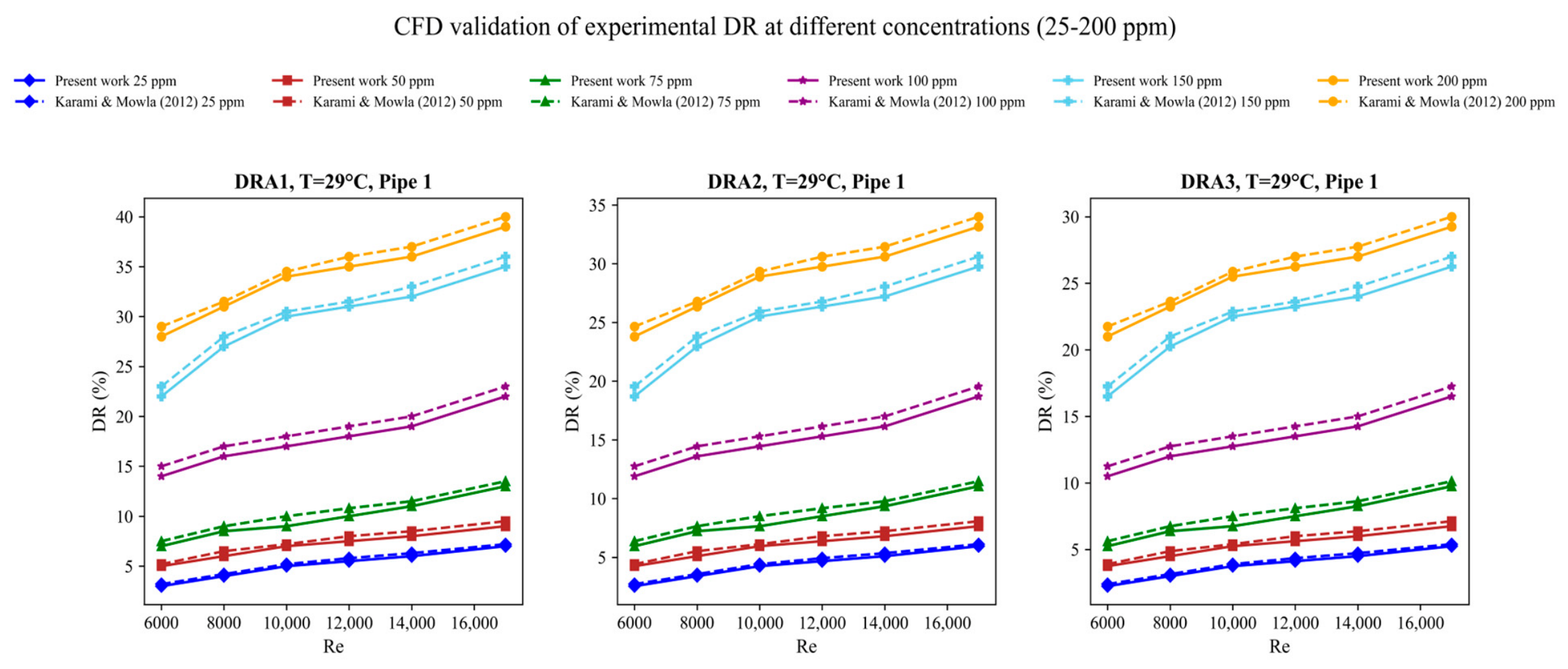
Figure 18 indicates the effect of DRA concentrations (25–200 ppm) on the drag reduction for pipe 1 at a temperature of 29 °C. For pipe 1: at 25 ppm, DR1 experimental DR values were 4, 5, 6, 7, and 8%, while the CFD validation values were 4.1, 5.2, 5.9, 7.2, and 7.9%. At 50 ppm, the experimental values were 5.5, 6, 6.5, 7, and 8, while the CFD values were 5, 5.5, 6, 6.5, 6.8, and 7.8. At 150 ppm, the experimental values were 12, 13, 14, 15, and 19%, while the CFD values were 12.5, 14, 16, and 20%. At 200 ppm, the experimental DR values were 26, 28, 31, 30, and 39%, the CFD values were 27.2, 29.3, 32, and 40.1%

Figure 18. CFD validation of experimental DR at different concentrations (25–200 ppm).

For pipe 2, at 25 and 50 ppm the experimental values were almost similar to the CFD values, while at 100 ppm, 150 ppm, and 200 ppm the experimental values were 14, 15, 14.5, 15, and 16%, 19, 20, 21, 22, and 23%, 21, 23, 25, and 27%, while the CFD validated values were 14.8, 15.7, 15.2, 16, and 17%, 20, 21, 22.1, 23.2, and 24%, 22, 24, 26, and 28%. For pipe 3, at 25, 50, 75, and 100 ppm the experimental values were approximately similar to the CFD values, but at 150 and 200 ppm the experimental values were 15, 17, 19, 18, and 20%, 19, 21, 23, 22, and 25%, while the CFD values we are 16, 17.1, 20, 19.1, and 21%, 20, 22, 24, 23, and 26.2%.

At elevated DRA concentrations, the ±10–15% drag-reduction (DR, %) deviations mainly arise because the power-law model captures only shear-thinning viscosity and neglects polymer elasticity, extensional viscosity, relaxation time, and finite chain extensibility. The SST k-ω further limits accuracy by using a linear eddy-viscosity assumption that cannot fully resolve anisotropic polymer-induced turbulence suppression.

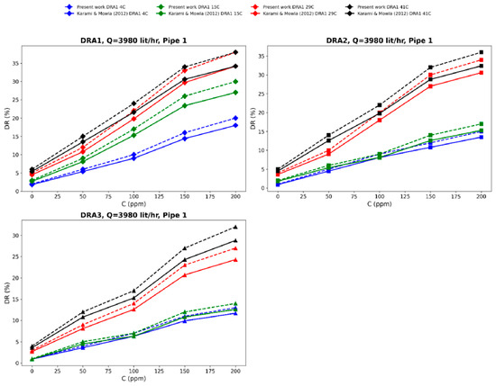
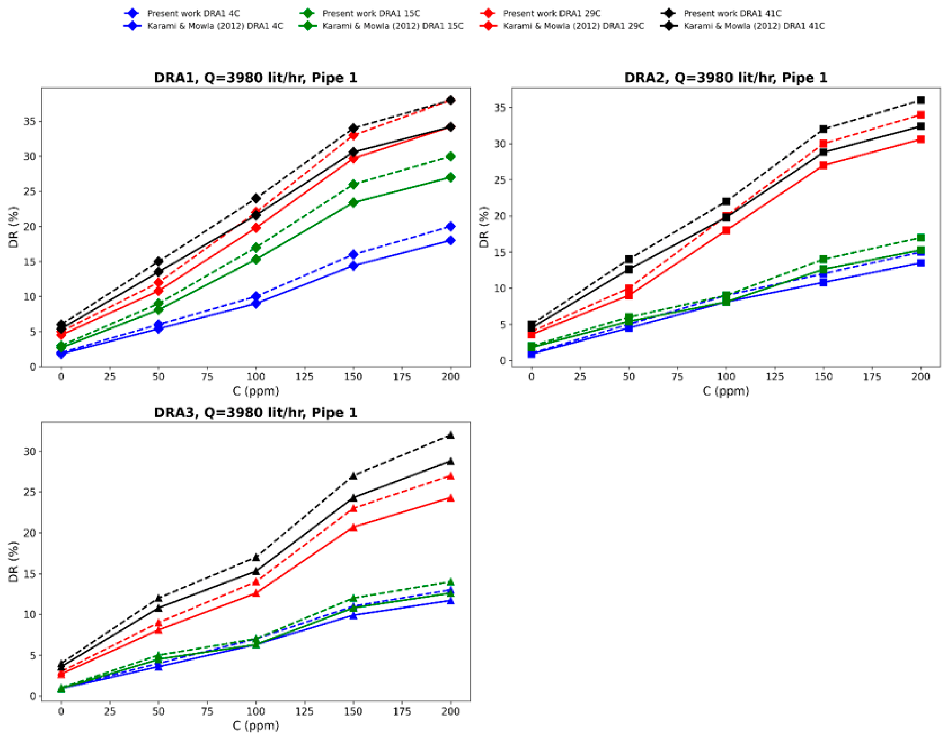
Figure 19 shows CFD validation of experimental drag reduction (DR %) at different DRA temperatures (i.e., 4 °C, 15 °C, 29°, and 41 °C) and a constant flow rate (3980 ${\displaystyle \frac{\mathrm{L}}{\mathrm{h}}}$). For DRA1, within the temperature range (4–41°) and concentration range (0–200) the experimental DR values were 2, 5, 8, 14, and 18%, 4, 8, 14.8, 24, and 28%, 4.9, 9.9, 18.8, and 24.9%, 6, 13, 16, 30, 35, and 36% for DR2, 2, 4.5, 7.5, and 14%, 4, 7, 16, 25, and 28%, while the CFD validated values for DRA1 are 2.5, 4.5, 9, 15, and 19%, 4, 8.3, 15.2, 25, and 29%, 4.9,0.3, 19.3, and 25.3%, 6, 14, 17, 31, 36.1, and 37.1%; for DRA2 they are 2, 4.7, 8.5, and 15%, 4, 8, 16.8, 26, and 29%, 5, 13, 19.2, 29.1, and 35.3%; and for DRA3 they are 2.5, 4.5, 9, 12.8, and 15.3%, 2.6, 5.2, 11, 15, and 25%.

Figure 19. CFD validation for experimental drag reduction (DR) at different concentrations of DRAs.

The CFD model reproduced the overall drag-reduction trend, but the discrepancy increases as polymer concentration and drag-reduction magnitude rise because the linear eddy-viscosity closure does not resolve polymer-induced Reynolds stress anisotropy, turbulent kinetic-energy redistribution, or near-wall vortex attenuation. Moreover, the absence of polymer-stress transport prevents simulation of the nonlinear exchange between polymer elastic energy and turbulent fluctuations. Since DR is derived from a pressure ratio, these modelling errors are amplified in the reported percentage.

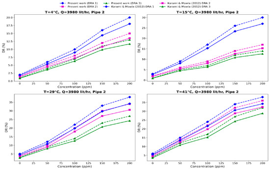
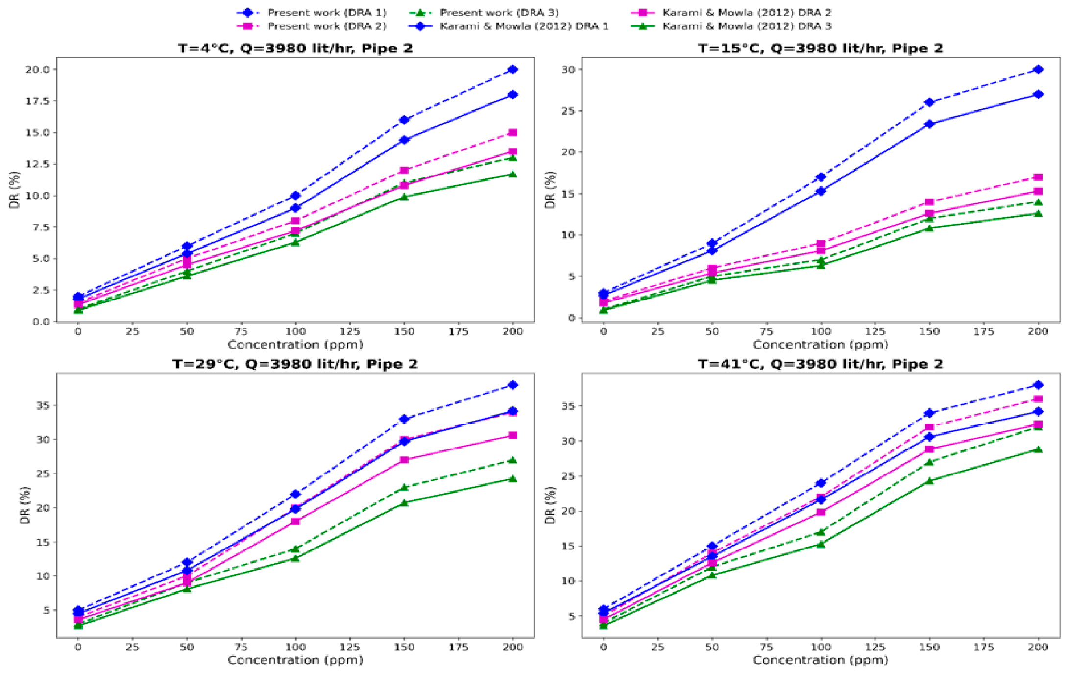
Figure 20 shows the effect of CFD validation of experimental DR (%) for various concentrations of DRAs (0–200 ppm) and a fixed flow rate f. For DRA3, DRA2, and DRA1 at 4 °C, the experimental DR (%) values were 1, 2.6, 6.5, 10, and 11.7, 2, 4.9, 6.6, 10.1, and 12.4, 2.4, 5, 8, 13, and 18, while the CFD values were 1, 2.8, 7.5, 11.2, and 12, 2, 5, 7.7, and 11.2, 2.5, 6, 9, and 14. At 15 °C, the experimental values were 1, 4.9, 5.2, 9.3, and10.2, 2, 4.9, 7, 12, and 14, 3.6, 8.3, 14.5, 24, and 26, while the CFD values were 1, 5.5, 6.3, 10, and 11, 2, 5, 8, and 13.1, 3.6, 9.4, 15, 25, and 27. At 29 °C, the experimental values were 2, 7, 9, 19, and 21, 3, 8, 16, 18, and 23, 3, 8, 16, 26, and 30, 5, 10, 18, 28, and 34, while the CFD values were 2, 8, 10, 20.1, and 22, 3, 9, 17, 19, and 24, 3, 9, 17.1, 27.1 and 31, 5, 11.1, 19.2, 29.1, and 35.2. At 41 °C, the experimental values were 2.5, 8, 13, 21, and 25, 4.5, 12, 18, 28, and 32, 5, 12, 18, and 33, while the CFD validated values were 2.5, 9, 14, 22, and 26, 4.5, 13, 19, 29, and 33, 5, 13.1, 19.1, and 34.2.

Figure 20. CFD validation of experimental DR (%) for various concentrations of DRAs (i.e., 0–200 ppm).

The increased CFD–experimental deviations at higher DRA concentrations can be attributed to shear-induced polymer-chain scission, which reduces the effective molecular weight, relaxation time, and drag-reduction efficiency during experiments. SST k-ω model assumes a homogeneous solution with constant rheological properties and therefore does not represent polymer degradation or concentration non-uniformity. This difference becomes pronounced near the maximum drag-reduction asymptote, where DR responds nonlinearly to small changes in polymer elasticity and molecular integrity.

5.4. CFD-Based Advanced Turbulence Reduction

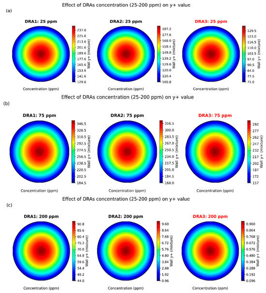
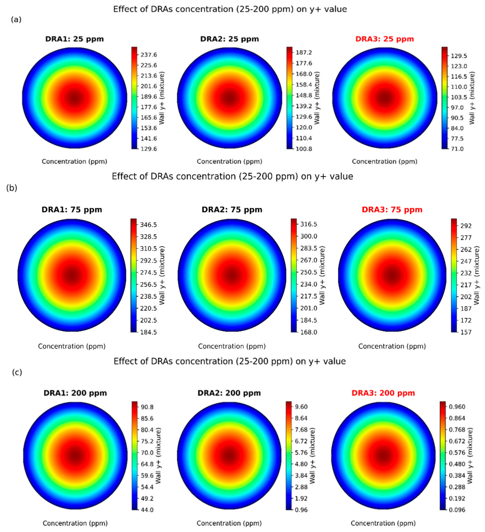
Figure 21 presents the effects of drag-reducing agent (DRA1, DRA2, and DRA3) concentrations (25, 75, and 200 ppm) on wall y plus value. At 25 ppm, the wall y⁺ ranges DRA1: 130–246, DRA2: 101–192, and DRA3: 71–135, showing that DRA3 achieves the finest near-wall resolution within the log-layer, improving wall shear stress and convective mass transfer accuracy. At 75 ppm, Y⁺ increases due to a thicker boundary layer, with DRA1: 185–355, DRA2: 168–323, and DRA3: 157–301, where DRA3 maintains more uniform wall gradients and mitigates excessive wall function reliance. This ensures more accurate simulation of turbulent momentum and scalar transport under high solute loading. At 200 ppm, y⁺ values are reduced for high diffusivity effects, with DRA1: 44–93, DRA2: 63–143, and DR3: 74–173.

Figure 21. (a–c) Effect of DRA concentrations (DRA1, DRA2, and DRA3) (25 ppm, 75 ppm, 200 ppm) on y⁺ value.

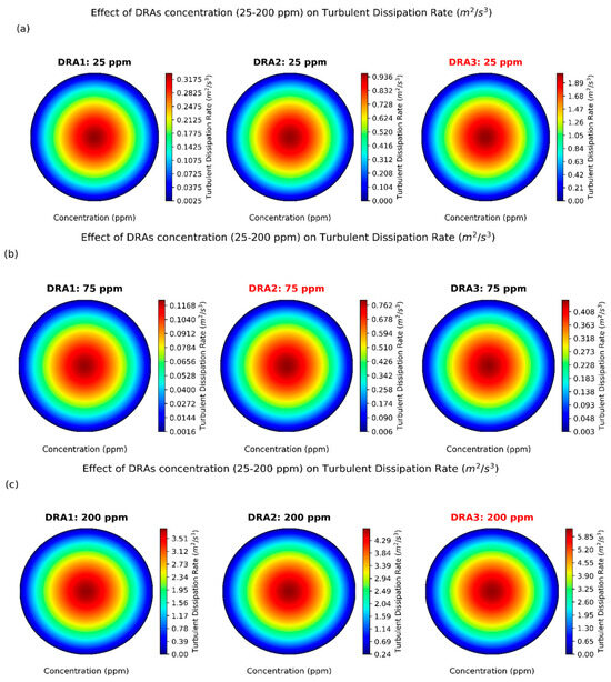
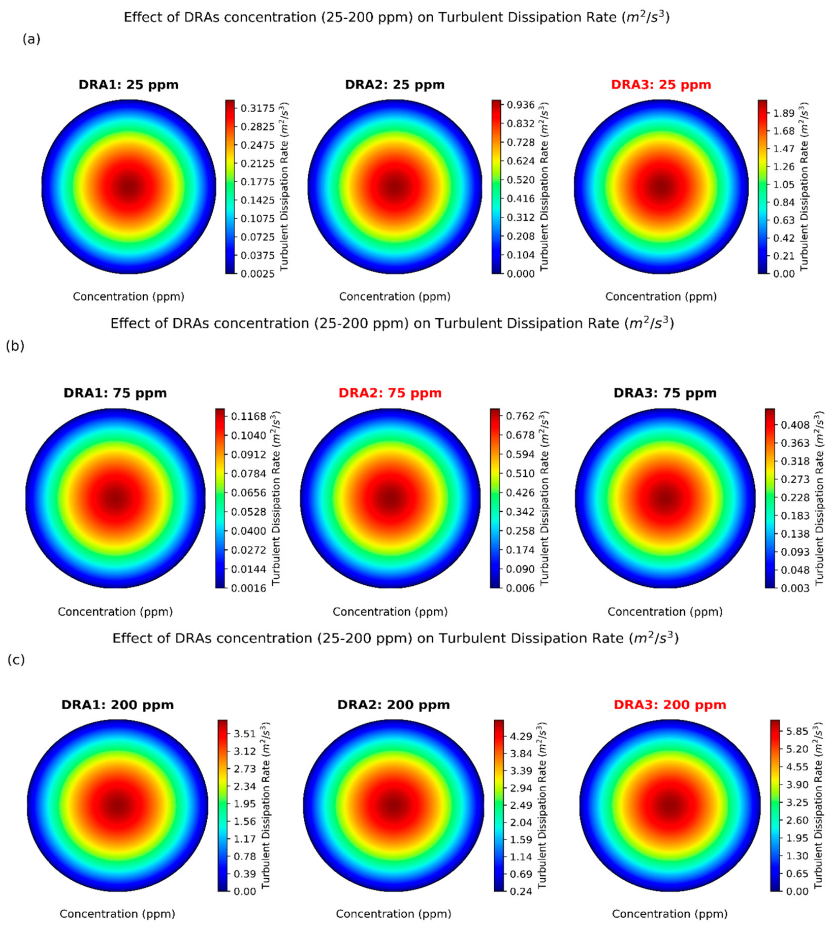
Figure 22 shows the effects of DRA concentrations (25, 75, and 200 ppm) on the turbulent dissipation rate (${\displaystyle \frac{{\mathrm{m}}^2}{{\mathrm{s}}^3}}$). At 25 ppm, the turbulent dissipation rate ranged from 3.09 × 10⁻³–3.32 × 10⁻¹ (${\displaystyle \frac{{\mathrm{m}}^2}{{\mathrm{s}}^3}}$) for DRA1, 6.68 × 10⁻³–9.58 × 10⁻¹ (${\displaystyle \frac{{\mathrm{m}}^2}{{\mathrm{s}}^3}}$) for DRA2, and 1.13 × 10⁻²–2.04 (${\displaystyle \frac{{\mathrm{m}}^2}{{\mathrm{s}}^3}}$) for DRA3. The contour shows a clear increase in dissipation intensity from DRA1 to DRA3 due to a weak velocity gradient and higher turbulence-damping effect. At 75 ppm, the turbulence dissipation rate varied from 1.53 × 10⁻³–1.21 × 10⁻¹ (${\displaystyle \frac{{\mathrm{m}}^2}{{\mathrm{s}}^3}}$)for DRA1, 7.15 × 10⁻³–7.92 × 10⁻¹ (${\displaystyle \frac{{\mathrm{m}}^2}{{\mathrm{s}}^3}}$) for DRA2, and 4.54 × 10⁻³–4.46 × 10⁻¹ (${\displaystyle \frac{{\mathrm{m}}^2}{{\mathrm{s}}^3}}$) for DRA3. At 200 ppm, the maximum turbulent dissipation rate increased from 3.81 (${\displaystyle \frac{{\mathrm{m}}^2}{{\mathrm{s}}^3}}$) for DRA1, 4.71 (${\displaystyle \frac{{\mathrm{m}}^2}{{\mathrm{s}}^3}}$) for DRA2, 6.25 for DRA3. The higher central dissipation observed for DRA3 indicates stronger turbulent energy dissipation compared with DRA1 and DRA2.

Figure 22. (a–c) Effect of drag-reducing agent concentrations (i.e., 25, 75, and 200 ppm) on the turbulent dissipation rate (${\displaystyle \frac{{\mathrm{m}}^2}{{\mathrm{s}}^3}}$).

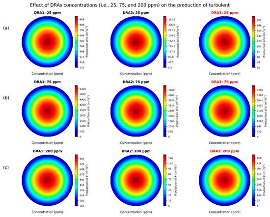
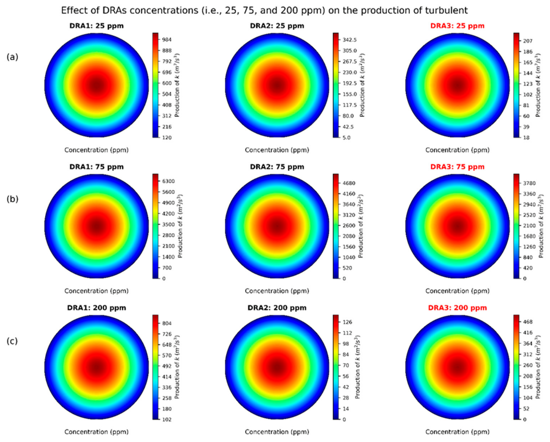
Figure 23 depicts the effect of DRA concentrations on the production of turbulent kinetic energy (k). At 25 ppm, the production of kinetic energy (k) is highest for DRA3 = 2.21 × 10³ ${\displaystyle \frac{\mathrm{k}\mathrm{g}}{\mathrm{m}{\mathrm{s}}^3}}$, followed by DRA1 = 1.04 × 10³ ${\displaystyle \frac{\mathrm{k}\mathrm{g}}{\mathrm{m}{\mathrm{s}}^3}}$, and DRA2 = 3.64 × 10² ${\displaystyle \frac{\mathrm{k}\mathrm{g}}{\mathrm{m}{\mathrm{s}}^3}}$. This shows that DRA3 produces stronger turbulence at low concentration due to higher local shear, stronger Reynolds stress interaction, and larger velocity gradient effects. At 75 ppm, all DRAs show a major increase (DRA1 = 6.74 × 10³ ${\displaystyle \frac{\mathrm{k}\mathrm{g}}{\mathrm{m}{\mathrm{s}}^3}}$, DRA2 = 5.09 × 10³ ${\displaystyle \frac{\mathrm{k}\mathrm{g}}{\mathrm{m}{\mathrm{s}}^3}}$, and DRA3 = 4.12 × 10³ ${\displaystyle \frac{\mathrm{k}\mathrm{g}}{\mathrm{m}{\mathrm{s}}^3}}$) while at maximum concentration of 200 ppm, the values drop to DRA1 = 8.82 × 10², DRA2 = 1.35 × 10², and DRA3 = 4.97 × 10² ${\displaystyle \frac{\mathrm{k}\mathrm{g}}{\mathrm{m}{\mathrm{s}}^3}}$. The variation suggests that turbulence production peaks around 75 ppm, but at the higher concentration of 200 ppm, the DRA molecules cause the reduction of irrotational flow and weakens eddy formation, damping velocity fluctuations by lowering the energy transfer from mean flow to turbulence.

Figure 23. (a–c) Effect of DRA concentrations (25, 75, and 2000 ppm) on the production of turbulent kinetic energy (k).

Figure 24 presents the effect of different types of DRAs and crude-oil pipe flow temperature (i.e., 4 °C, 15 °C, 29 °C, and 41 °C). At the 4 °C, PPR increases from DRA1 to DRA3, with maximum values rising from 26.8 W to 38 W. The highest reduction occurs at the pipe core, while lower values near the wall reflect stronger viscous resistance. At 15 °C, PPR increases to 31.8 W, 39.2 W, and 43 W for DRA1, DRA2, and DRA3, respectively. DRA3 provides the most effective turbulence suppression and energy savings (30%). At 29 °C, PPR is 37.8 W for DRA1, 45.2 W for DRA2, and 51.0 for DRA3. The enlarged high-reduction core region indicates improved polymer–turbulence interaction at the higher temperature. At 41 °C, the highest PPR is obtained, reaching 40.9 W, 51.0 W, and 55.0 W for DRA1, DRA2, and DRA3, respectively. DRA3 exhibits the strongest overall PPR in comparison to DRA1 and DRA2.

5.5. Energy Reduction in Crude-Oil Pipeline System

Figure 25 indicates the energy savings (ES) potential at different DRAs (i.e., DRA1, DRA2, DRA3) and temperatures (4 °C, 15 °C, 29 °C, and 41 °C). ES increases with DRAs (DRA1, DRA2, and DRA3) with an increase in temperature from 4 °C to 41 °C. For DRA1 ES improves from 1.5–3% to 17–23% with an increase in temperature from 4 °C to 41 °C. For DRA2 ES rises from about 2.0–3.5% to 20–27% as the temperature increases from 4 °C to 41 °C, the maximum ES potential happens for DRA3, it increases from 2.5–4% to 23–30%. ES increases due to the drag-reduction effect, near-wall turbulence eddies, and Reynolds shear stress, producing a reduction in ∆p and hence in PPR.

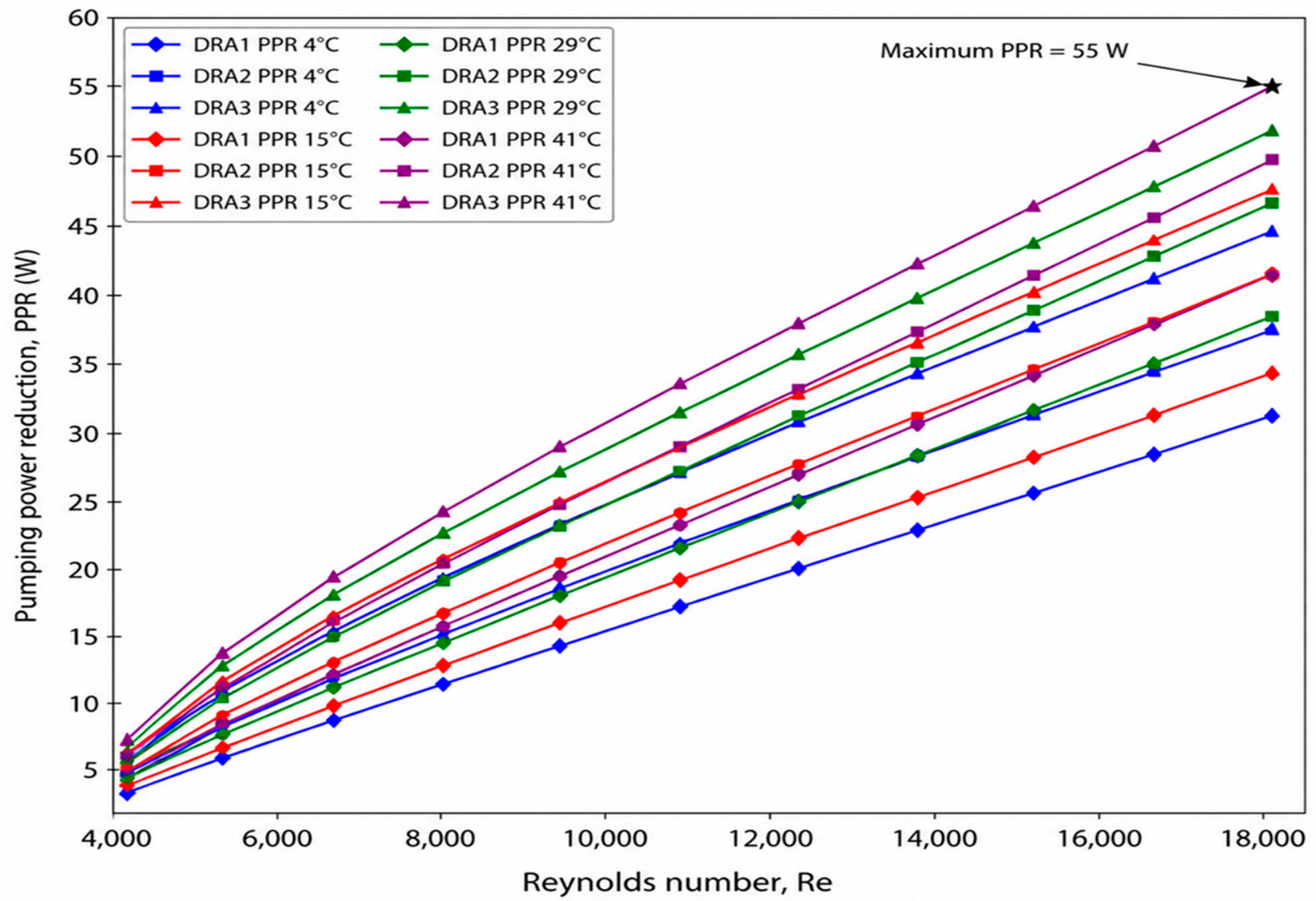
Figure 26 shows the effect of drag-reducing agent (DRA) temperatures (4–41 °C) on pumping power reduction (PPR) at various Reynolds numbers (2.5 × 10³–2 × 10⁴). PPR increases almost linearly with the increase in DRA types and temperatures (4–41 °C). For DRA1, PPR rises from approximately 2–4 W to 32–42 W, while for DRA2 it increases from about 2.5–4.5 W to 38–50 W. DRA3 provides the highest reduction, increasing from approximately 3–5 W to 45–55 W, with the maximum 55 W at 41 °C at Reynolds number 1.8 × 10⁴. DRA3 performs well at 41 °C: it stretches along the flow direction and dampens turbulent bursts, streamwise vortices, and velocity fluctuations, thereby reducing the effective friction factor and wall shear stress.

Figure 24. (a–d) Effect of DRA types and pipe flow temperatures on pumping power reduction.

Figure 24. (a–d) Effect of DRA types and pipe flow temperatures on pumping power reduction.

Figure 25. Energy saving (ES %) at different temperatures (4–41 °C) and Reynolds numbers (4 × 10³–1.8 × 10⁴).

Figure 25. Energy saving (ES %) at different temperatures (4–41 °C) and Reynolds numbers (4 × 10³–1.8 × 10⁴).

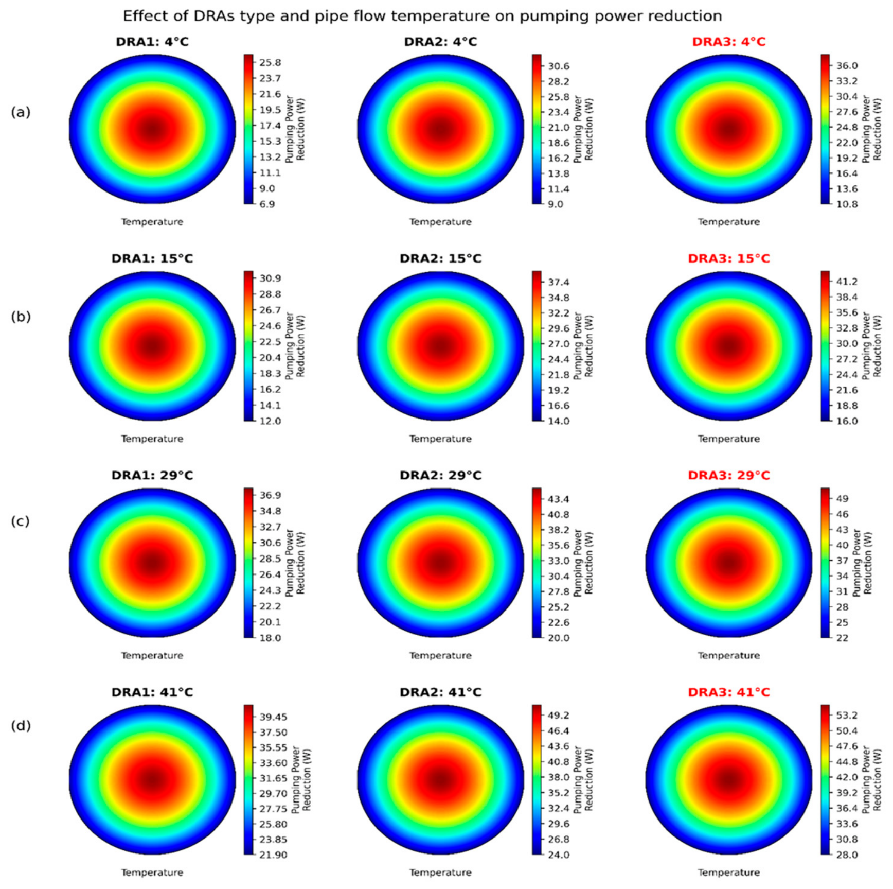
Figure 26. Effect of drag-reducing agent (DRA) temperatures (4–41 °C) on pumping power reduction (W) at various Reynolds numbers (4 × 10³–1.8 × 10⁴).

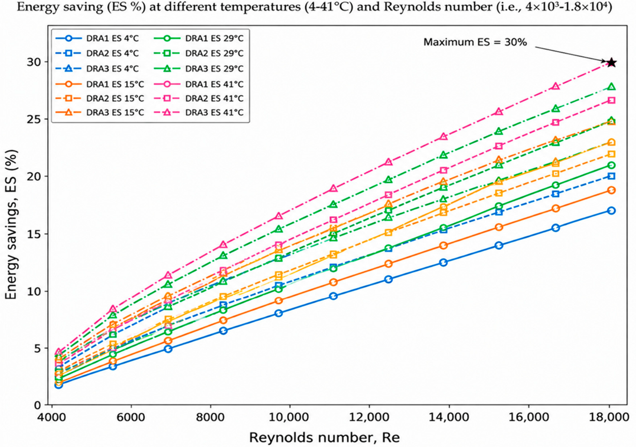
Figure 26. Effect of drag-reducing agent (DRA) temperatures (4–41 °C) on pumping power reduction (W) at various Reynolds numbers (4 × 10³–1.8 × 10⁴).

6. Conclusions

This study established an integrated CFD-ML framework for simultaneous prediction of pressure drop (∆p), drag reduction (DR), pumping power reduction (PPR), energy savings (ES), and flow-rate enhancement in DRA-assisted crude-oil pipelines. Among the investigated conditions (25–200 ppm), DRA3 delivered the best performance, achieving a maximum DR of 44.2%, PPR of 55 W, ES of 30%, and flow-rate enhancement 5–10 (${\displaystyle \frac{\mathrm{L}}{\mathrm{d}\mathrm{a}\mathrm{y}}}$) relative to the baseline. At 200 ppm and 41 °C, improved near-wall reduced y⁺ value from 246 to 1, while the turbulent dissipation rate increased from 0.332 to 6.25 and turbulent kinetic energy decreased from 1040 (${\displaystyle \frac{\mathrm{k}\mathrm{g}}{{\mathrm{m}\mathrm{s}}^3}}$) to 497 (${\displaystyle \frac{\mathrm{k}\mathrm{g}}{{\mathrm{m}\mathrm{s}}^3}}$), demonstrating pronounced appearance of near-wall turbulent activity. The validated SST k-ω model provided detailed resolution of near-wall flow, shear stress transport, and pressure losses, whereas the KAN model achieved a higher coefficient of performance (R² = 0.9318) for PPR and effectively captured nonlinear interactions among DRA characteristics, pipe geometry, and operating conditions. The key novelty of the proposed work is the coupling of high-fidelity CFD with KAN-based spline learning, enabling both physics-based and rapid prediction of hydraulic and energy performance indicators within a unified framework. These findings demonstrate the potential of the proposed approach for optimizing DRA-assisted pipeline operation and reducing pumping-energy demands.

Challenges and Perspectives

Despite the promising performance of the proposed CFD-ML framework, several challenges and research gaps remain before it can be applied more broadly to industrial pipeline systems. Firstly, broad experimental and field-scale validation is required. Future studies should test the CFD-KAN framework over wider ranges of Reynolds numbers, temperature, pressure, pipe geometry, roughness, and crude-oil properties to confirm its robustness under realistic industrial conditions. Secondly, DRA chemistry and long-term polymer stability need further investigation. The effects of molecular weight, structure, solubility, and mechanical or thermal degradation should be assessed for synthetic, bio-based, and natural DRAs. Thirdly, more complex pipeline configurations should be considered.

The present framework should be extended to vertical, inclined, curved, and varying diameter pipes, as well as gas–liquid and oil–water–polymer multiphase flow systems. Fourthly, ML generalization should be improved using larger and more diverse datasets. Future studies should combine CFD, experimental, and real-time crude-oil industrial data, and it should be compared and analyzed with a KAN-ensemble algorithm involving a Gaussian neural network (GNN) and other physics-guided learning approaches. Finally, real-time optimization and digital twin applications should be explored. Integrating CFD-ML models with continuous operational data could optimize DRA dosage, flow rate, and pumping conditions while minimizing energy consumption and pressure losses.

References

- Obiomah, F. Pipeline Transportation of Hydrocarbons, 1st ed.; researchgate.net; TSL logistics Nigeria: Lagos, Nigeria, 2025; pp. 1–48. [Google Scholar]
- Alhamd, S.J.; Rashid, F.L.; Al-Obaidi, M.A.; Aldami, A.K. Unveiling crude oil viscosity and rheological Properties: An experimental comparison of Nano silica and Nano Molybdenum disulfide in Bazargan Oilfield. Fuel 2025, 381, 133698. [Google Scholar] [CrossRef] [Scilit]
- Li, N.-L.; Chen, B. Evaluation of frictional pressure drop correlations for air-water and air-oil two-phase flow in pipeline-riser system. Pet. Sci. 2024, 21, 1305–1319. [Google Scholar] [CrossRef] [Scilit]
- Shadloo, M.S.; Rahmat, A. Estimation of pressure drop of two-phase flow in horizontal long pipes using artificial neural networks. J. Energy Resour. Technol. 2020, 142, 112110. [Google Scholar] [CrossRef] [Scilit]
- Foggi Rota, G.; Monti, A.; Rosti, M.E. Saving energy in turbulent flows with unsteady pumping. Sci. Rep. 2023, 13, 1299. [Google Scholar] [CrossRef] [Scilit] [PubMed]
- Subrahmanyam, M.A.; Cantwell, B.J.; Alonso, J.J. A universal velocity profile for turbulent wall flows including adverse pressure gradient boundary layers. J. Fluid Mech. 2022, 933, A16. [Google Scholar] [CrossRef] [Scilit]
- Toms, B.A. Some observations on the flow of linear polymersolutions through straight tubes at large Reynolds numbers. In Proceedings of the First International Congress on Rheology; North-Holland Publishing Co.: Amsterdam, The Netherlands, 1949; Volume 2, pp. 135–141. [Google Scholar]
- Virk, P.S.; Merrill, E.W. The Toms phenomenon: Turbulent pipe flow of dilute polymer solutions. J. Fluid Mech. 1967, 30, 305–328. [Google Scholar] [CrossRef] [Scilit]
- AL-Dogail, A.; Gajbhiye, R.; Patil, S. A review of drag-reducing agents (DRAs) in petroleum industry. Arab. J. Sci. Eng. 2023, 48, 8287–8305. [Google Scholar] [CrossRef] [Scilit]
- Khamehchi, E.; Dargi, M.; Imeri, M.; Mahdavi Kalatehno, J.; Khaleghi, M.R. Pipe diameter optimization and two-phase flow pressure drop in seabed pipelines: A genetic algorithm approach. Interciencia 2023, 48, 82–100. [Google Scholar] [CrossRef] [Scilit]
- Baakeem, S.S.; Hashlamoun, K.; Hethnawi, A.; Mheibesh, Y.; Nassar, N.N. Drag reduction by polymer additives: State-of-the-art advancements in experimental and numerical approaches. Ind. Eng. Chem. Res. 2024, 63, 7485–7506. [Google Scholar] [CrossRef] [Scilit]
- Hussein, E.Q.; Rashid, F.L.; Al-Obaidi, M.A.; Ameen, A.; Chilbani, A.; Kezzar, M.; Mahariq, I. Optimising Drag-Reducing Agent Performance for Energy-Efficient Pipeline Transport. Energies 2026, 19, 812. [Google Scholar] [CrossRef] [Scilit]
- Baccouch, M. Computational Fluid Dynamics-Analysis, Simulations, and Applications: Analysis, Simulations, and Applications, 1st ed.; IntechOpen: London, UK, 2025; pp. 1–209. [Google Scholar]
- Liu, S.; Hu, H.; Xie, L.; Deng, H.; Zhang, L.; Wen, J. Experimental investigation on flow-induced vibration suppression by drag-reducing polymers. Phys. Fluids 2025, 37, 083130. [Google Scholar] [CrossRef] [Scilit]
- Khamees, L.A.; Abdul-Majeed, G.H.; Alhaleem, A.A. A review of improving the heavy crude oil transportation process using additives. J. Chem. Pet. Eng. 2025, 59, 291–338. [Google Scholar]
- Li, D.; Chen, Y. Fluid drag reduction assisted by machine learning: A review. Phys. Fluids 2026, 38, 011304. [Google Scholar] [CrossRef] [Scilit]
- Sagar, T.; Kumar, S.; Patel, D.K.; Nandan, G.; Sharma, V.K. Artificial Intelligence-Enhanced Developments in Computational Fluid Dynamics. In Artificial Intelligence and Computational Modeling in Heat Transfer and Fluid Dynamics, 1st ed.; Awasti, M.K., Gupta, R., Eds.; Wiley: Hoboken, NJ, USA; II MT University: Meerut, India, 2026; pp. 51–92. [Google Scholar]
- Schnack, D.D. Mass conservation and the equation of continuity. In Lectures in Magnetohydrodynamics: With an Appendix on Extended MHD; Springer: Berlin/Heidelberg, Germany, 2009; pp. 19–24. [Google Scholar]
- Rennels, D.C. Pipe Flow: A Practical and Comprehensive Guide, 2nd ed.; John Wiley Sons: Hoboken, NJ, USA, 2022; pp. 1–343. [Google Scholar]
- Anderson, J.D.; Wendt, J. Computational Fluid Dynamics; Springer: Berlin/Heidelberg, Germany, 1995; Volume 206, p. 332. [Google Scholar]
- Fox, R.W.; McDonald, A.T.; Mitchell, J.W. Fox and McDonald’s Introduction to Fluid Mechanics, 9th ed.; John Wiley & Sons: Verdun, France, 2016; pp. 1–672. [Google Scholar]
- Pokrovskii, V.N. The Mesoscopic Theory of Polymer Dynamics, 1st ed.; Springer: Berlin/Heidelberg, Germany; University of Malta: Msida, Malta, 2002; pp. 81–113. [Google Scholar]
- Kim, S.; Kamrin, K. Power-law scaling in granular rheology across flow geometries. Phys. Rev. Lett. 2020, 125, 088002. [Google Scholar] [CrossRef] [Scilit] [PubMed]
- Yao, J.; Rezaeiravesh, S.; Schlatter, P.; Hussain, F. Direct numerical simulations of turbulent pipe flow up to Reτ ≈ 5200. J. Fluid Mech. 2023, 956, A18. [Google Scholar]
- Loyseau, X.F.; Verdin, P.G.; Brown, L. Scale-up and turbulence modelling in pipes. J. Pet. Sci. Eng. 2018, 162, 1–11. [Google Scholar] [CrossRef] [Scilit]
- Grioni, M.; Elaskar, S.; Bruel, P.; Mirasso, A. Numerical Simulation of Turbulent Flows using the SST-SAS Model. WSEAS Trans. Fluid Mech. 2024, 19, 24–39. [Google Scholar] [CrossRef] [Scilit]
- Könözsy, L. The k-ω shear-stress transport (SST) turbulence model. In A New Hypothesis on the Anisotropic Reynolds Stress Tensor for Turbulent Flows: Volume I: Theoretical Background and Development of an Anisotropic Hybrid k-Omega Shear-Stress Transport/Stochastic Turbulence Model; Springer: Berlin/Heidelberg, Germany, 2019; Volume 120, pp. 57–66. [Google Scholar]
- Wilcox, D.C. Turbulence Modeling for CFD; DCW industries: La Canada, CA, USA, 1998; Volume 2. [Google Scholar]
- Tomaszewska-Wach, B.; Ligus, G. Assessment of the Impact of k-ε and k-ω Turbulence Models on the Compatibility of CFD Simulations with PIV Measurements for Flow Through a Measuring Orifice. Appl. Sci. 2025, 15, 12204. [Google Scholar] [CrossRef] [Scilit]
- Fiorillo, F.; Esposito, L.; Ginolfi, M.; Leone, G. New insights into turbulent and laminar flow relationships using Darcy–Weisbach and Poiseuille laws. Water 2024, 16, 1452. [Google Scholar] [CrossRef] [Scilit]
- Alfonsi, G. Reynolds-averaged Navier–Stokes equations for turbulence modeling. Appl. Mech. Rev. 2009, 62, 040802. [Google Scholar] [CrossRef] [Scilit]
- Karami, H.; Mowla, D. Investigation of the effects of various parameters on pressure drop reduction in crude oil pipelines by drag reducing agents. J. Non-Newton. Fluid Mech. 2012, 177, 37–45. [Google Scholar] [CrossRef] [Scilit]
- Yusuf, S.N.A.; Asako, Y.; Sidiq, N.A.C. A short review on rans turbulence models. CFD Lett. 2020, 12, 83–96. [Google Scholar] [CrossRef] [Scilit]
- Jin, Q.; Ma, C.; Su, Y.; Han, H.; Zhang, L. Transient field predictions for oscillating pipe flow cooling with Reynolds averaged Navier–Stokes equations informed neural networks. Int. J. Heat Fluid Flow 2026, 121, 110545. [Google Scholar]
- Rahman, M.; Vuorinen, V.; Taghinia, J.; Larmi, M. Wall-distance-free formulation for SST k-ω model. Eur. J. Mech.-B/Fluids 2019, 75, 71–82. [Google Scholar] [CrossRef] [Scilit]
Disclaimer/Publisher’s Note: The statements, opinions and data contained in all publications are solely those of the individual author(s) and contributor(s) and not of MDPI and/or the editor(s). MDPI and/or the editor(s) disclaim responsibility for any injury to people or property resulting from any ideas, methods, instructions or products referred to in the content. |
© 2026 by the authors. Licensee MDPI, Basel, Switzerland. This article is an open access article distributed under the terms and conditions of the Creative Commons Attribution (CC BY) license.