Inverse Acoustic Localization of Pile-Driving Noise from Synchronized Multi-Receiver SPL Measurements

Abstract

Construction noise assessment commonly assumes that the source location is already known, which limits its applicability when active equipment cannot be accessed or precisely surveyed. This study proposes a transparent inverse acoustic model for jointly estimating the location and time-dependent sound pressure level (SPL) of a pile-driving source from synchronized field measurements. Noise was recorded for 5 s at five GNSS-defined receiver positions on a construction site in Astana, Kazakhstan, producing 40 SPL values per receiver at 0.125 s intervals. The model applied spherical geometrical spreading and identified the source position by minimizing the disagreement among the distance-corrected source levels obtained from the receivers. The source was estimated at local coordinates [56.6, 113.8] m, with a Monte Carlo sensitivity analysis indicating a 95% confidence region of approximately 5–8 m under combined receiver-coordinate and SPL-measurement uncertainty. Its reconstructed SPL ranged from 81.6 to 99.9 dB(A) at the 1 m reference distance, while the equivalent source SPL was 90.4 dB(A). The measured impulsive pattern was preserved in the reconstructed source history, with dominant peaks occurring at approximately 1 s intervals. Comparison of measured and predicted receiver levels yielded an overall MAE of 1.3 dB(A) and RMSE of 1.6 dB(A), reflecting internal consistency between measured and reconstructed receiver levels. The as-driven pile position was subsequently surveyed independently, giving a true localization error of 2.3 m for the estimated position, within the 95% confidence region above. Out-of-sample cross-validation and synthetic sweep across the search zone further characterize the method’s identifiability and its expected sensitivity away from the search-zone center.

1. Introduction

Construction activities are among the most variable and disruptive sources of environmental noise in urban areas because their location, duration, equipment composition, and operating conditions change continuously over the project lifecycle. Unlike comparatively stable transportation or industrial sources, construction noise is commonly intermittent, temporary, spatially mobile, and characterized by sudden peaks generated by impacts, material handling, excavation, and heavy machinery [1]. In densely developed areas, such emissions can disturb nearby communities and create operational, regulatory, and economic risks for contractors [2]. Objective measurements and resident surveys have shown that construction activities may dominate the local acoustic environment and produce substantially greater annoyance than other nearby sources [3]. Similar concerns have been reported for rail-transit construction, where combinations of drilling, impact equipment, compressors, pumps, and material-processing machinery caused location-dependent exceedances of applicable noise limits [4].

Pile driving represents a particularly challenging construction-noise source because it generates a sequence of short, high-energy impulses rather than a stationary acoustic signal. Controlled experiments have confirmed that pulsed sounds exhibit stronger short-term peaks and fluctuations than steady or blended sounds, while their measured levels decrease systematically with distance; in the experimental study [5], the median level declined from 72.7 dB at the source to 54.8 dB at 3 m, and the fitted attenuation relationship achieved R² = 0.8664. Although underwater and airborne propagation involve different physical media, offshore pile-driving research [6] also demonstrates the importance of measuring impulsive noise at several distances and validating propagation models against field data. Such work additionally highlights that a source level stated at a reference distance of 1 m should generally be interpreted as a normalized source-strength quantity obtained through propagation modelling, rather than necessarily as a directly measurable pressure level at a physical point exactly 1 m from an extended pile-driving source [7].

The propagation of outdoor sound is governed not only by distance but also by interactions with the ground, atmosphere, terrain, and surrounding objects. Ground impedance and source-receiver geometry can substantially alter attenuation through interference between direct and ground-reflected waves, particularly when propagation occurs close to porous or layered surfaces [8]. Wind and temperature gradients may refract acoustic waves, while turbulence, non-flat terrain, diffraction, and multiple reflections can cause deviations from ideal free-field behavior [9]. Comprehensive engineering models, such as Harmonoise, therefore represent propagation attenuation as a combination of geometrical divergence, atmospheric absorption, ground effects, diffraction, refraction, and turbulence-related contributions [10]. Nevertheless, when the propagation distance is moderate, the available field information is limited, and the purpose is rapid source identification rather than full spectral reconstruction, geometrical spreading provides a transparent first-order relationship between source strength, receiver level, and distance. Its simplification must, however, be recognized when interpreting residual errors caused by site-specific reflections, shielding, and ground effects.

Early quantitative studies of construction noise mainly treated the measured signal as a stochastic process and sought to predict its temporal variation or occupational exposure. Manatakis [11] modelled construction-equipment noise through regression-based functional expansions and expressed uncertainty using confidence and prediction zones. Manatakis and Skarlatos [12] subsequently related equivalent noise exposure to equipment flows, operating conditions, working-area characteristics, and source–receiver distance, reporting a standard error of approximately 2 dB(A) for their fitted construction-equipment model. These approaches established the importance of considering time-dependent variability, equipment operation, and distance, but their main objective was exposure prediction at known observation points rather than identification of an unknown source location.

Later studies increasingly incorporated construction sequencing, equipment uncertainty, and equivalent continuous sound levels into computer-based prediction. Zhang and Pei [13] developed a discrete-event simulation framework that accounts for the synchronization of several simultaneously operating sources, propagation attenuation, activity duration, and the energy-based calculation of equivalent continuous noise. Gilchrist et al. [2] used Monte Carlo simulation to predict noise levels around an urban construction site and validated the model against field measurements during different construction stages. Hong et al. [14] also applied Monte Carlo simulation to equipment-noise data and reported a difference of 2.76 dB(A) between predicted and measured construction-noise levels, with a correlation coefficient of 0.991. These studies demonstrate that physically interpretable propagation relationships can provide useful predictions when combined with realistic equipment information. However, they generally assume that the source or equipment locations are already known and then calculate the sound level at predetermined receivers.

Other research has focused on preventive construction-noise management at the planning stage. Kwon et al. [15] developed a case-based reasoning model that retrieved similar historical construction disputes using project, equipment, duration, distance, and neighborhood attributes. Ning et al. [16] incorporated noise exposure into multi-objective construction-site layout optimization together with transportation cost and safety risk. Kantová [17] demonstrated how construction-machine sources, receiver positions, noise barriers, and operational schedules can be represented in a preconstruction noise study, noting that advance modelling may prevent substantial extensions of construction time. Baek et al. [18] integrated construction-equipment scheduling with noise prediction and obtained an allowable prediction error rate of 3.83%; their case study indicated that alternative equipment allocations could reduce resident exposure by up to 4.4 dB or lower direct costs by 24.6%. These methods are valuable for planning and mitigation, but they rely predominantly on predefined source locations, equipment databases, schedules, or historical cases and are therefore not designed to locate an unregistered or spatially uncertain active source from simultaneous field measurements.

Recent developments have moved construction-noise assessment toward real-time sensing, spatial estimation, and data-driven modelling. Lee et al. [19] combined a noise-customized spatial interpolation model with an ISO 9613-based [20] propagation model incorporating geometrical divergence, atmospheric absorption, ground effects, obstacles, and source directivity. Their field evaluation produced RMSE values of 2.62 dB for noise inside the construction site and 2.70 dB for the surrounding area. Ooi et al. [21] integrated stochastic simulation with deep learning and validated the resulting construction-noise model through ten case studies, obtaining average absolute differences below 1.2 dB(A). A sensor- and GIS-based conceptual system has also been proposed for transmitting construction-noise measurements to a server, identifying sources and exceedance locations, and displaying the calculated distribution as an interactive heat map [22]. A subsequent review of construction-site vibroacoustic monitoring solutions concluded that current systems still face limitations associated with cost, accuracy, background-noise filtering, data processing, visualization, and adaptation to different site geometries and scales [23]. These findings indicate a continuing need for methods that can extract spatial source information from a small number of practical field instruments without requiring dense sensor deployment or extensive training datasets.

Sound-source localization has been studied extensively outside the construction-management field. Acoustic beamforming uses the phase and amplitude relationships measured by microphone arrays to focus on candidate source directions or positions, but its spatial resolution and susceptibility to side lobes depend on the array geometry, aperture, microphone number, frequency, and assumed propagation model [24]. In complex urban environments, Albert et al. [25] demonstrated numerically that time-reversal processing could localize an impulsive source using only three or eight non-line-of-sight sensors, although the approach required a finite-difference propagation model of the surrounding buildings and considerable computational effort. An et al. [26] incorporated direct and reflected acoustic paths into a three-dimensional localization method and reported an average distance error of approximately 0.8 m; considering reflected paths improved accuracy by about 40%, but the method required a microphone array and a reconstructed three-dimensional indoor environment. These studies show that reflections can either degrade localization when neglected or improve it when accurately modelled. A separate body of work formulates localization directly from received signal strength (RSS) rather than phase or arrival-time data, since RSS-based ranging avoids the inter-sensor clock synchronization that time-of-arrival methods require [27,28]. These methods are well established in wireless and underwater sensor networks but have seen limited application to airborne construction-noise sources measured with simple sound level meters.

Inverse acoustic approaches provide an alternative to conventional beamforming. Gombots et al. [29] formulated source localization by minimizing the difference between measured and finite-element-simulated sound pressures, enabling the geometry and boundary conditions of the measurement environment to be represented more accurately than with free-field steering vectors. Sun and Liu [30] applied sparse inverse reconstruction to spherical beamforming and obtained improved spatial resolution and background-noise suppression in numerical examples. More generally, Nelson and Yoon [31] showed that acoustic source-strength reconstruction depends strongly on the conditioning of the source-to-receiver transfer matrix, the numbers and spatial arrangements of sources and microphones, and the source-receiver separation. Yoon and Nelson [32] further demonstrated that Tikhonov regularization, singular-value discarding, and cross-validation can stabilize poorly conditioned inverse solutions. These advanced approaches provide high-resolution source maps and source-strength distributions, but they commonly require multi-channel waveform data, known transfer functions, phase information, detailed environmental models, or regularization procedures.

The reviewed literature reveals a separation between two major research directions. Construction-noise models usually predict sound levels, exposure, costs, or mitigation requirements after source locations and equipment characteristics have been specified, whereas established acoustic-localization methods generally depend on microphone arrays, waveform timing, phase differences, directional information, or detailed numerical representations of the propagation environment. Comparatively little attention has been given to a simpler inverse field problem in which the construction-noise source position is unknown and must be jointly estimated with its time-varying acoustic strength using only synchronized scalar SPL measurements from several spatially distributed sound level meters. The present work therefore extends the RSS-based localization paradigm to construction-noise monitoring: its novelty lies not in the propagation model itself, which is a standard spherical spreading relationship, but in the joint estimation of a time-varying source strength alongside position from low-cost, non-array sound level meter data, applied specifically to impulsive pile-driving noise.

Accordingly, this study aims to develop and field-test a transparent inverse mathematical model for locating an unknown pile-driving source and estimating its time-dependent SPL from simultaneous short-term measurements at five GNSS-defined receiver positions. The model treats pile driving as a fixed-point source over the considered 5 s interval, allows its source SPL to vary at 0.125 s time steps, and searches the construction-site area for the position that minimizes the disagreement among the distance-corrected source-level estimates obtained from the five receivers. The selected formulation intentionally prioritizes simplicity, physical interpretability, and practical field implementation over a detailed representation of reflections, ground impedance, meteorological refraction, or spectral directivity. The field application demonstrates that the proposed procedure can produce a distinct source-location estimate, reconstruct the impulsive source-level history, and reproduce the measured receiver levels with low prediction errors; Section 3.5 further quantifies how sensitive that estimate is to plausible input uncertainty, and independent verification against ground-truth source coordinates remains an important next step.

2. Materials and Methods

2.1. Field Measurements

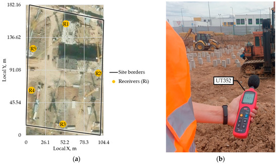
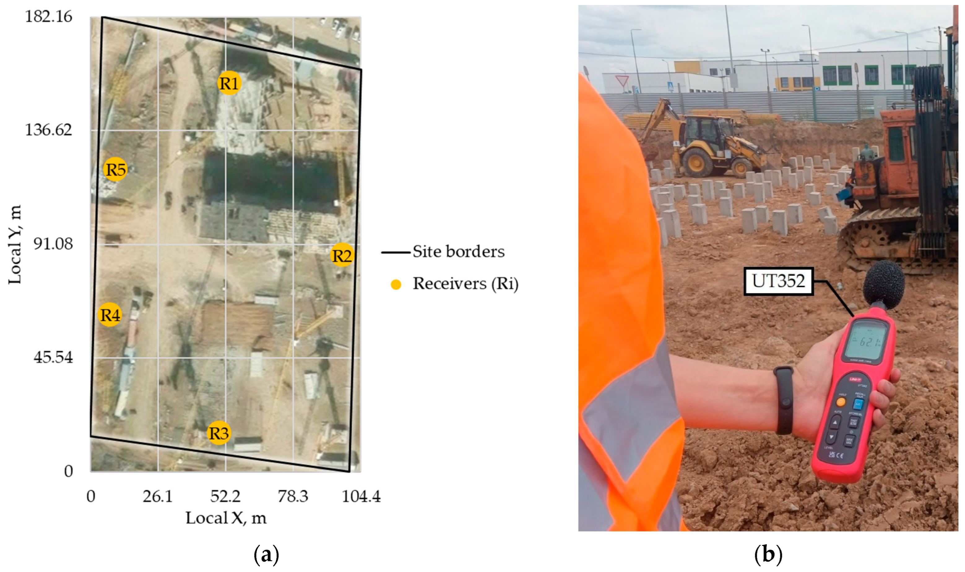
Field measurements were conducted at an active construction site in Astana, Kazakhstan, during pile-driving works (Figure 1). The purpose of the measurements was to obtain short-term SPL records at several surrounding points and use them to inversely determine the approximate location and acoustic strength of the pile-driving source.

Figure 1. Field measurement setup: (a) study area and spatial arrangement of the five sound receiver positions; (b) SPL measurement using the UT352 sound level meter.

As shown in Figure 1a, five measurement positions (R1, R2, R3, R4, and R5) were arranged around the construction activity. The preliminary geographic coordinates of each position were determined using a GNSS receiver and converted into the local metric coordinate system. At each position, the SPL was measured using a UT352 sound level meter (UNI-T, Dongguan, China) (Figure 1b). The measurement area was open and unobstructed, with a clear line of sight between the pile-driving source and all five receiver positions; no buildings, fences, stockpiles, parked equipment, or significant terrain features were present along any of the direct source-to-receiver paths. Measurements were taken with the UT352 configured to A-weighting, FAST time response (0.125 s per reading), auto range mode, over the instrument’s 30–130 dB range (±1.5 dB accuracy, 31.5–8000 Hz frequency response). The microphone was held at a height of 1 m above ground level during all recordings. The instrument was factory-calibrated by the manufacturer shortly before the field measurements were conducted. Since the device does not provide automatic data logging at a selected sampling frequency, the screen of each sound level meter was video-recorded during the measurement period using smartphones, following the general approach of [5]. To establish a common time reference across the five independently filmed devices, all recordings used the same video application, which overlays a real-time clock timestamp derived from each smartphone’s network-synchronized system clock onto every frame. The SPL readings were subsequently extracted by matching each receiver’s video to this common absolute timestamp, rather than by aligning frame counts or elapsed recording time alone (Appendix A Table A1). Because the UT352 was configured to FAST time response, its displayed value updates at the same 8 Hz rate as the internal sampling, so each timestamped reading corresponds to a distinct instrument sample rather than an arbitrarily chosen instant during a continuously changing display. This procedure reduces, though does not entirely eliminate, timing uncertainty arising from network clock precision, video frame rate, and video compression; the residual synchronization error is expected to be a small fraction of the 0.125 s sampling interval, well below the ≥1-sample propagation-delay effect discussed in Section 4.

The measurement duration was 5 s. The values were copied with a time interval of 0.125 s, corresponding to 8 records per second. Thus, each measurement position produced 40 SPL values. The measurements at the five positions were carried out simultaneously, so that the recorded values could be compared at the same time steps.

The measured dataset can be written as:

$$\left[{\mathrm{L}}_{\mathrm{i},\mathrm{k}}^{\mathrm{m}\mathrm{e}\mathrm{a}\mathrm{s}}\right],$$

(1)

where ${\mathrm{L}}_{\mathrm{i},\mathrm{k}}^{\mathrm{m}\mathrm{e}\mathrm{a}\mathrm{s}}$ is the measured SPL at receiver $\mathrm{i}$ and time step $\mathrm{k}$, with $\mathrm{i}$ = 1, 2, 3, 4, 5 and $\mathrm{k}$ = 1, 2, …, 40. All SPL values reported in this study are A-weighted levels referenced to 20 µPa (dB(A)), consistent with the operating mode of the UT352 sound level meter.

2.2. Coordinate Preparation

The latitude and longitude of the five measurement positions were converted into a local Cartesian coordinate system using an ellipsoidal equirectangular projection referenced to the mean latitude of the site (WGS84), with the origin placed at the minimum easting/northing among the five receivers. This was required because the mathematical model operates with distances between points. Each receiver was therefore represented by horizontal coordinates:

$${\mathrm{R}}_{\mathrm{i}}=\left({\mathrm{x}}_{\mathrm{i}},{\mathrm{y}}_{\mathrm{i}}\right),$$

(2)

where ${\mathrm{R}}_{\mathrm{i}}$ is the position of receiver $\mathrm{i}$, and ${\mathrm{x}}_{\mathrm{i}}$ and ${\mathrm{y}}_{\mathrm{i}}$ are its coordinates in meters.

The unknown pile-driving source was represented as:

$$\mathrm{S}=\left({\mathrm{x}}_{\mathrm{s}},{\mathrm{y}}_{\mathrm{s}}\right),$$

(3)

where ${\mathrm{x}}_{\mathrm{s}}$ and ${\mathrm{y}}_{\mathrm{s}}$ are the unknown coordinates of the sound source. The model assumes that the source position remains constant during the short 5 s measurement interval, while its SPL may vary with time because pile driving is an impulsive and non-stationary process [33].

The distance (${\mathrm{r}}_{\mathrm{i}}$) between the source and receiver $\mathrm{i}$ is calculated as:

$${\mathrm{r}}_{\mathrm{i}}=\sqrt{{({\mathrm{x}}_{\mathrm{i}}-{\mathrm{x}}_{\mathrm{s}})}^2+{({\mathrm{y}}_{\mathrm{i}}-{\mathrm{y}}_{\mathrm{s}})}^2},$$

(4)

2.3. Sound Propagation Model

The proposed outdoor sound propagation model assumes that the sound level decreases mainly due to geometrical spreading. Therefore, for a point-like construction noise source (i.e., pile driving activity), the SPL at a receiver, i.e., the measured SPL (${\mathrm{L}}_{\mathrm{i},\mathrm{k}}^{\mathrm{m}\mathrm{e}\mathrm{a}\mathrm{s}}$), can be written as:

$${\mathrm{L}}_{\mathrm{i},\mathrm{k}}^{\mathrm{m}\mathrm{e}\mathrm{a}\mathrm{s}}={\mathrm{L}}_{\mathrm{s},\mathrm{k}}-20{\log }_{10}\left({\displaystyle \frac{{\mathrm{r}}_{\mathrm{i}}}{{\mathrm{r}}_0}}\right)-\mathsf{\alpha }\left({\mathrm{r}}_{\mathrm{i}}-{\mathrm{r}}_0\right)+{\mathsf{\epsilon }}_{\mathrm{i},\mathrm{k}},$$

(5)

where ${\mathrm{L}}_{\mathrm{s},\mathrm{k}}$ is the unknown source SPL at reference distance ${\mathrm{r}}_0$, taken as 1 m; $\mathsf{\alpha }$ is the atmospheric attenuation coefficient in dB/m; ${\mathsf{\epsilon }}_{\mathrm{i},\mathrm{k}}$ is the residual error.

The term $20{\log }_{10}\left({\displaystyle \frac{{\mathrm{r}}_{\mathrm{i}}}{{\mathrm{r}}_0}}\right)$ describes the reduction in SPL caused by spherical spreading [34]. The atmospheric attenuation term $\mathsf{\alpha }\left({\mathrm{r}}_{\mathrm{i}}-{\mathrm{r}}_0\right)$ may be included when the distances are large enough for air absorption to be relevant. For relatively short construction-site distances, this term may be set to zero or kept as a small correction parameter. The reference distance ${\mathrm{r}}_0$ was set to 1 m to express the estimated source SPL as a normalized source-strength value. This does not imply that the SPL was measured at 1 m from the pile-driving source; rather, it provides a fixed reference distance for back-calculating and comparing source levels. Since ${\mathrm{r}}_0$ is constant for all receivers, its selection does not influence the estimated source location but only defines the reference scale of ${\mathrm{L}}_{\mathrm{s},\mathrm{k}}$.

In the present study, $\mathsf{\alpha }$ was set to zero because the measurement distances were relatively short and detailed meteorological correction was outside the scope of the field test. It should be noted that atmospheric absorption is frequency-dependent, and pile-driving impulses contain broadband energy; since the UT352 sound level meter applies A-weighting rather than resolving individual frequency bands, the reported SPL values represent an integrated, frequency-weighted quantity rather than a narrowband signal, and no attempt was made to back out a single equivalent broadband $\mathsf{\alpha }$ from these measurements. Standardized procedures such as ISO 9613-2 and ANSI/ASA S1.26 provide frequency-resolved methods for atmospheric absorption when such detail is required [20,35]. Thus, when atmospheric attenuation is neglected, the model becomes:

$${\mathrm{L}}_{\mathrm{i},\mathrm{k}}^{\mathrm{m}\mathrm{e}\mathrm{a}\mathrm{s}}={\mathrm{L}}_{\mathrm{s},\mathrm{k}}-20{\log }_{10}\left({\displaystyle \frac{{\mathrm{r}}_{\mathrm{i}}}{{\mathrm{r}}_0}}\right)+{\mathsf{\epsilon }}_{\mathrm{i},\mathrm{k}},$$

(6)

This simplified form was selected because it is transparent, physically understandable, and suitable for inverse estimation when only a limited number of receivers is available.

2.4. Inverse Determination of Source Location

The main task of the mathematical model is to determine the unknown source position $\mathrm{S}$ and the corresponding source SPL value ${\mathrm{L}}_{\mathrm{s},\mathrm{k}}$. Since the distance to the source is unknown, the model searches for the source position that makes the measurements from all receivers most consistent with one common source level.

For any assumed source position, the measured SPL at each receiver can be recalculated back to the source reference distance. The back-calculated SPL from receiver $\mathrm{i}$ at time step $\mathrm{k}$ is:

$${\mathrm{L}}_{\mathrm{s},\mathrm{i},\mathrm{k}}={\mathrm{L}}_{\mathrm{i},\mathrm{k}}^{\mathrm{m}\mathrm{e}\mathrm{a}\mathrm{s}}+20{\log }_{10}\left({\displaystyle \frac{{\mathrm{r}}_{\mathrm{i}}}{{\mathrm{r}}_0}}\right),$$

(7)

If the assumed source position is correct, then all five receivers should give approximately the same back-calculated source level at the same time step. Therefore, for each time step $\mathrm{k}$, the estimated SPL is calculated as the average of the five back-calculated values:

$${\overline{\mathrm{L}}}_{\mathrm{s},\mathrm{k}}={\displaystyle \frac{1}{\mathrm{n}}}{\displaystyle {\sum }_{\mathrm{i}=1}^{\mathrm{n}}}{\mathrm{L}}_{\mathrm{s},\mathrm{i},\mathrm{k}},$$

(8)

where $\mathrm{n}$ is the number of receivers ($\mathrm{n}$ = 5 in our case).

The consistency error for a candidate source position is then calculated as:

$$\mathrm{J}\left({\mathrm{x}}_{\mathrm{s}},{\mathrm{y}}_{\mathrm{s}}\right)={\sum }_{\mathrm{k}=1}^{\mathrm{m}}{\sum }_{\mathrm{i}=1}^{\mathrm{n}}{\left({\mathrm{L}}_{\mathrm{s},\mathrm{i},\mathrm{k}}-{\overline{\mathrm{L}}}_{\mathrm{s},\mathrm{k}}\right)}^2,$$

(9)

where $\mathrm{m}$ is the number of time steps ($\mathrm{m}=40$ in our case). The optimal source position is the position that minimizes this error:

$$\left({\mathrm{x}}_{\mathrm{s}}^{\ast },{\mathrm{y}}_{\mathrm{s}}^{\ast }\right)=\arg \underset{{\mathrm{x}}_{\mathrm{s}},{\mathrm{y}}_{\mathrm{s}}}{\min }\mathrm{J}\left({\mathrm{x}}_{\mathrm{s}},{\mathrm{y}}_{\mathrm{s}}\right)$$

(10)

This means that the selected source location is the point for which the five receivers produce the most similar source SPL values after distance correction. The inverse localization model was applied within the rectangular search zone (i.e., study area shown in Figure 1a) with dimensions of 104.4 m × 182.16 m. The search zone was bounded by the coordinates [0, 0] and [104.4, 182.16] m. The objective function $\mathrm{J}\left({\mathrm{x}}_{\mathrm{s}},{\mathrm{y}}_{\mathrm{s}}\right)$ was calculated for the possible source positions inside this zone, and the point corresponding to the minimum objective-function value was selected as the most probable location of the pile-driving source.

2.5. Estimation of Source SPL

After the optimal source coordinates $\left({\mathrm{x}}_{\mathrm{s}}^{\ast },{\mathrm{y}}_{\mathrm{s}}^{\ast }\right)$ are found, the distance from this source position to each receiver is recalculated:

$${\mathrm{r}}_{\mathrm{i}}^{\ast }=\sqrt{{\left({\mathrm{x}}_{\mathrm{i}}-{\mathrm{x}}_{\mathrm{s}}^{\ast }\right)}^2+{\left({\mathrm{y}}_{\mathrm{i}}-{\mathrm{y}}_{\mathrm{s}}^{\ast }\right)}^2}$$

(11)

Then, for every time step, the source SPL is estimated as:

$${\mathrm{L}}_{\mathrm{s},\mathrm{k}}^{\ast }={\displaystyle \frac{1}{\mathrm{n}}}\sum _{\mathrm{i}=1}^{\mathrm{n}}\left[{\mathrm{L}}_{\mathrm{i},\mathrm{k}}^{\mathrm{m}\mathrm{e}\mathrm{a}\mathrm{s}}+20{\log }_{10}\left({\displaystyle \frac{{\mathrm{r}}_{\mathrm{i}}^{\ast }}{{\mathrm{r}}_0}}\right)\right]$$

(12)

The obtained sequence (${\mathrm{L}}_{\mathrm{s},1}^{\ast },{\mathrm{L}}_{\mathrm{s},2}^{\ast },\dots ,{\mathrm{L}}_{\mathrm{s},40}^{\ast }$) represents the estimated time-varying SPL of the pile-driving source at the reference distance of 1 m. Since pile driving produces impulsive sound, the source SPL is not treated as a constant value. Instead, it is estimated separately for each 0.125 s interval.

For an integral description of the source over the full 5 s interval, the equivalent source SPL can be calculated as:

$${\mathrm{L}}_{\mathrm{s},\mathrm{e}\mathrm{q}}=10{\log }_{10}\left[{\displaystyle \frac{1}{\mathrm{m}}}\sum _{\mathrm{k}=1}^{\mathrm{m}}{10}^{{\displaystyle \frac{{\mathrm{L}}_{\mathrm{s},\mathrm{k}}^{\ast }}{10}}}\right]$$

(13)

This value describes the average acoustic energy of the source during the measurement period.

2.6. Reconstruction Consistency Check

To assess the reconstruction consistency of the inverse model, the estimated source position and source SPL values were used to calculate predicted SPL values (${\widehat{\mathrm{L}}}_{\mathrm{i},\mathrm{k}}$) at the receiver positions:

$${\widehat{\mathrm{L}}}_{\mathrm{i},\mathrm{k}}={\mathrm{L}}_{\mathrm{s},\mathrm{k}}^{\ast }-20{\log }_{10}\left({\displaystyle \frac{{\mathrm{r}}_{\mathrm{i}}^{\ast }}{{\mathrm{r}}_0}}\right)$$

(14)

The predicted SPL values were compared with the measured SPL values. The model error at each receiver was calculated as:

$${\mathrm{e}}_{\mathrm{i},\mathrm{k}}={\mathrm{L}}_{\mathrm{i},\mathrm{k}}^{\mathrm{m}\mathrm{e}\mathrm{a}\mathrm{s}}-{\widehat{\mathrm{L}}}_{\mathrm{i},\mathrm{k}},$$

(15)

where ${\mathrm{L}}_{\mathrm{i},\mathrm{k}}^{\mathrm{m}\mathrm{e}\mathrm{a}\mathrm{s}}$ is the measured SPL and ${\widehat{\mathrm{L}}}_{\mathrm{i},\mathrm{k}}$ is the predicted SPL.

The mean absolute error (MAE) was calculated as:

$$\mathrm{M}\mathrm{A}\mathrm{E}={\displaystyle \frac{1}{\mathrm{n}\mathrm{m}}}\sum _{\mathrm{i}=1}^{\mathrm{n}}\sum _{\mathrm{k}=1}^{\mathrm{m}}\left|{\mathrm{e}}_{\mathrm{i},\mathrm{k}}\right|$$

(16)

The root mean square error (RMSE) was calculated as:

$$\mathrm{R}\mathrm{M}\mathrm{S}\mathrm{E}=\sqrt{{\displaystyle \frac{1}{\mathrm{n}\mathrm{m}}}\sum _{\mathrm{i}=1}^{\mathrm{n}}\sum _{\mathrm{k}=1}^{\mathrm{m}}{\mathrm{e}}_{\mathrm{i},\mathrm{k}}^2}$$

(17)

These indicators were used to evaluate how accurately the identified source location and source SPL reproduce the measured SPL at the five surrounding positions.

2.7. Sensitivity and Uncertainty Analysis

To assess how uncertainty in the input data and in the assumed propagation exponent affects the inverse model, three complementary analyses were performed. First, the receiver coordinates were perturbed with independent, zero-mean Gaussian noise (${\mathsf{\sigma }}_{\mathrm{r}}$ = 3 m per horizontal coordinate, representative of the accuracy achievable with a hand-held GNSS receiver), and the source position was re-estimated for each of 1000 realizations following the same procedure as in Section 2.4. Second, the measured SPL values were perturbed with independent, zero-mean Gaussian noise (${\mathsf{\sigma }}_{\mathrm{L}}$ = 1.5 dB, matching the manufacturer-specified accuracy of the UT352), and both the source position and the source SPL time history (Equation (12)) were re-estimated for each of 1000 realizations. Third, a combined perturbation applying both sources of noise simultaneously was performed. For each ensemble, the 95% confidence region of the estimated source position was obtained from the eigenvalues of the covariance matrix of the resulting (${\mathrm{x}}_{\mathrm{s}}$, ${\mathrm{y}}_{\mathrm{s}}$) estimates, assuming an approximately bivariate-normal distribution. Finally, the sensitivity of the estimated source position to the assumed exponent was evaluated by replacing the coefficient of 20 in Equations (6)–(9) with $10\mathrm{n}$, where $\mathrm{n}$ is a general path-loss exponent, and repeating the deterministic inversion for $\mathrm{n}$ in the range 1.5–3.0.

2.8. Main Assumptions of the Model

The proposed model is based on several assumptions. First, the pile-driving noise source is represented as a single dominant point source. Second, the source position is assumed to be fixed during the 5 s measurement period. Third, the source SPL is allowed to vary with time, which reflects the impulsive nature of pile driving. Fourth, the main mechanism of SPL reduction is assumed to be geometrical spreading. Additional effects, including ground reflection, shielding by temporary structures, scattering from nearby buildings, wind influence, and local reflections, are included in the residual error term. Fifth, the source and receivers are treated as coplanar, and the vertical offset between the pile-driving impact point (which itself changes as the pile advances into the ground) and the ground-level receiver positions is neglected; the resulting bias is quantified in Section 4.

These assumptions make the model simple enough for practical use with a limited number of measurement points, while still preserving the main physical relationship between sound level and distance. The model is therefore suitable for rapid field-based estimation of construction noise source location and source strength when direct access to the source position is limited or when the exact distance to the source is unknown.

3. Results

3.1. Overview of Measured Sound Pressure Levels

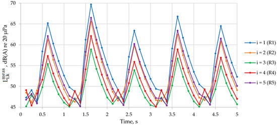
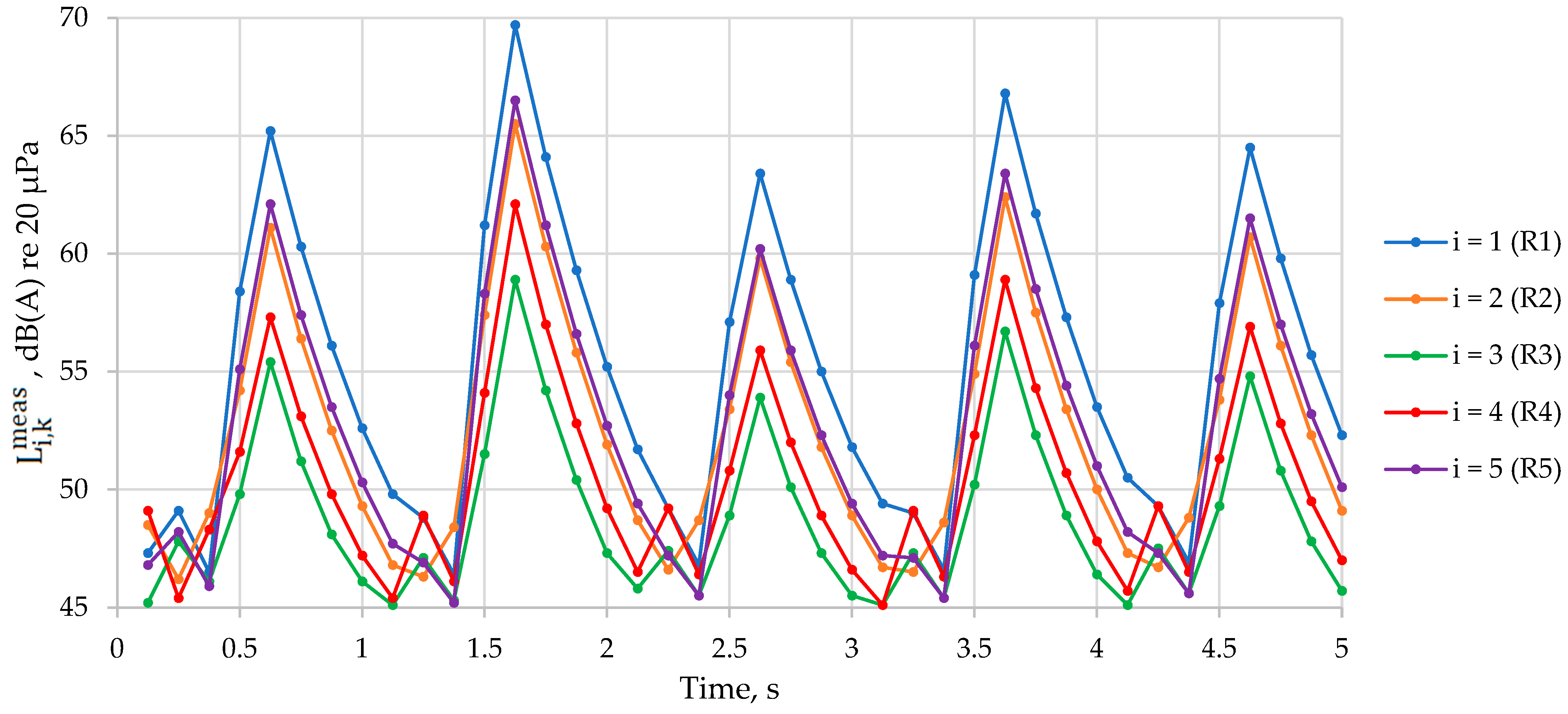
The 5 s measurement campaign produced 40 synchronized SPL records at each of the five receivers (Figure 2). The time histories at all receivers exhibited a similar cyclic pattern, with repeated short-term increases and decreases in SPL, which is consistent with the impulsive nature of pile-driving operations. The dominant peaks were observed at approximately 0.625, 1.625, 2.625, 3.625, and 4.625 s, indicating a quasi-periodic impact sequence with an interval of about 1 s between major impulses.

Figure 2. Time histories of measured SPL at the five receivers.

Among the five receivers, R1 recorded the highest SPL values, with a maximum measured value of 69.7 dB(A), whereas R3 recorded the lowest overall levels, with a maximum of 58.9 dB(A). The equivalent SPL values over the 5 s interval followed the same pattern (Table 1), indicating that the source was located closer to R1, R5, and R2 than to R3 and R4.

Table 1. Summary statistics of measured SPL at the five receivers.

Receiver	Minimum SPL, dB(A) Re 20 µPa	Maximum SPL, dB(A) Re 20 µPa	Equivalent SPL, dB(A) Re 20 µPa
R1	46.4	69.7	59.8
R2	46.2	65.5	55.9
R3	45.1	58.9	50.6
R4	45.1	62.1	52.8
R5	45.2	66.5	56.7

3.2. Estimated Source Location and Source-to-Receiver Distances

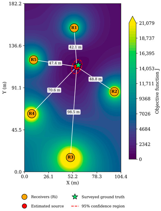
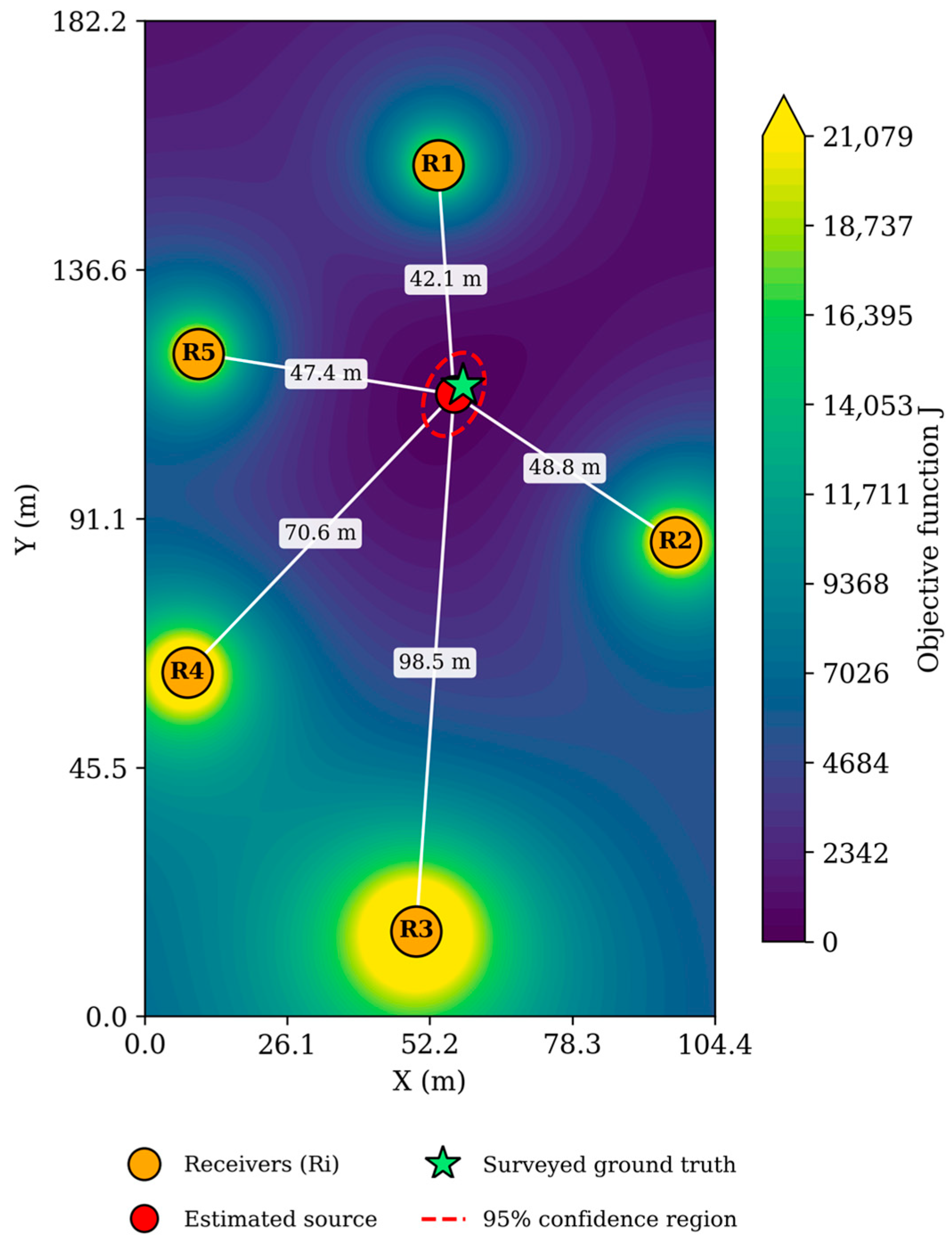
Figure 3 presents the objective-function map together with the estimated source location, receiver positions, and source-to-receiver distance lines. The orange circles indicate the receiver positions, the red circle indicates the estimated source location, and the green star indicates the independently surveyed ground-truth position (Section 3.2). The contour background shows the spatial variation in the objective function $\mathrm{J}\left({\mathrm{x}}_{\mathrm{s}},{\mathrm{y}}_{\mathrm{s}}\right)$, where the lowest region corresponds to the most consistent source position according to the inverse model. The distance lines provide a visual interpretation of the spatial relationship between the estimated source and each receiver.

Figure 3. Objective-function map, estimated source location, surveyed ground-truth position, and 95% confidence region (combined receiver-coordinate and SPL-measurement uncertainty).

As shown in Figure 3, the source was estimated to be located in the central part of the search zone, between the five receiver positions. The minimum value of the objective function $\mathrm{J}\left({\mathrm{x}}_{\mathrm{s}},{\mathrm{y}}_{\mathrm{s}}\right)$ was obtained at ${\mathrm{x}}_{\mathrm{s}}^{\ast }$ = 56.6 m and ${\mathrm{y}}_{\mathrm{s}}^{\ast }$ = 113.8 m. This result is consistent with the measured SPL distribution, since the highest equivalent SPL values were recorded at R1, R5, and R2, while the lowest value was recorded at R3, which was the farthest receiver from the estimated source. The calculated distances from the estimated source to the receivers were 42.1 m for R1, 48.8 m for R2, 98.5 m for R3, 70.6 m for R4, and 47.4 m for R5. These distances confirm that R3 had the largest source-to-receiver separation, which explains its comparatively lower measured SPL values. In contrast, R1, R2, and R5 were located at relatively similar distances from the estimated source, which is also reflected in their higher measured and equivalent SPL values.

The as-driven position of the pile was subsequently surveyed using the same GNSS receiver and measurement procedure applied to the five sound-level-meter positions (WGS84 Longitude of 71.392422 and Latitude of 51.165247), providing an independent ground-truth reference for the estimated source location (local coordinates [58.2, 115.4] m). Comparison against this reference gives a localization error of 2.3 m for the source position reported above ([56.6, 113.8] m), within the 95% confidence region reported in Section 3.5 (semi-axes of approximately 5–8 m).

3.3. Estimated Source SPL

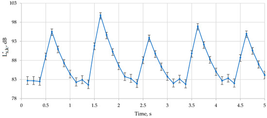
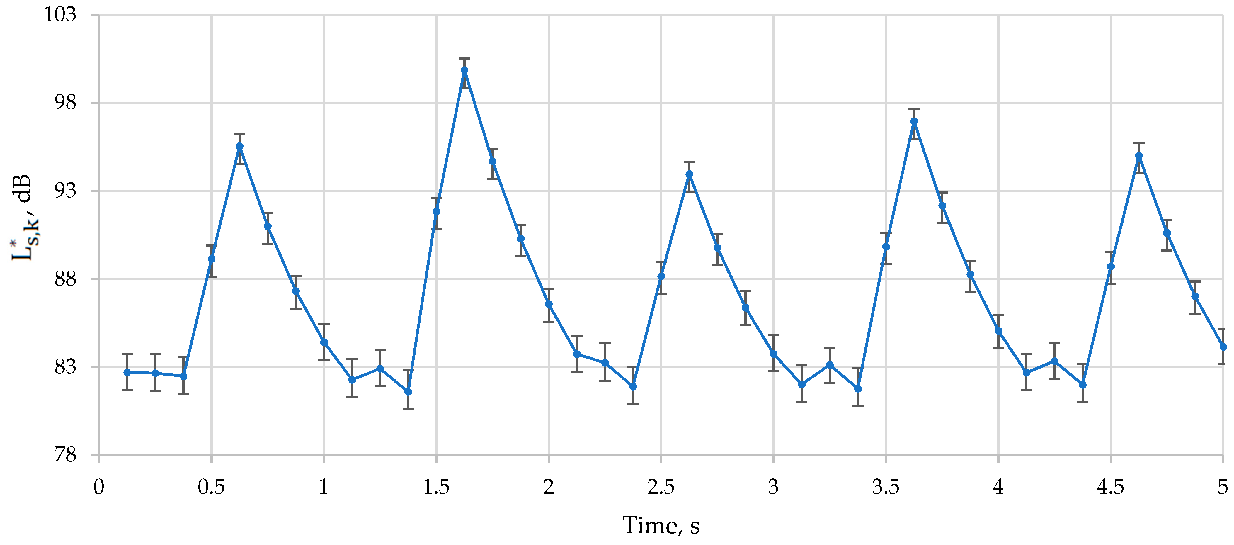
After determination of the optimal source location, the source SPL was back-calculated for each time step $\mathrm{k}$. The resulting source-level time history also exhibited a pronounced impulsive pattern (Figure 4). The estimated source SPL varied from 81.6 dB(A) to 99.9 dB(A) at the reference distance of 1 m, with an arithmetic mean of 87.2 dB(A). The highest estimated source SPL occurred at 1.625 s, corresponding to the strongest impact event observed simultaneously at all receivers.

Figure 4. Estimated source SPL time history, with error bars representing ±1 standard deviation from a level-dependent SPL-measurement Monte Carlo perturbation (Section 3.5), which are visibly wider during quiet intervals between pile-driving pulses.

The equivalent source SPL over the full 5 s interval was 90.4 dB(A). This value characterizes the mean acoustic energy of the pile-driving source during the considered short-term event. The repeated peaks in the source-level time history confirm that the recorded sound field was governed not by stationary background noise, but by a sequence of dominant pile-driving impulses. The strongest source peaks were observed at approximately 0.625 s (95.5 dB(A)), 1.625 s (99.9 dB(A)), 2.625 s (94 dB(A)), 3.625 s (97 dB(A)), and 4.625 s (95 dB(A)).

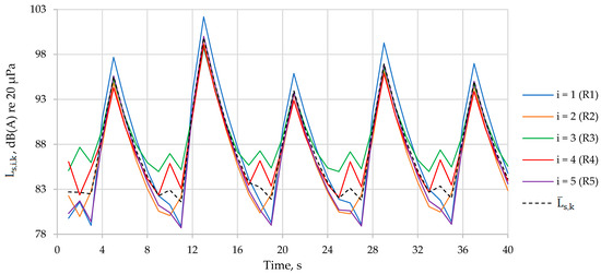
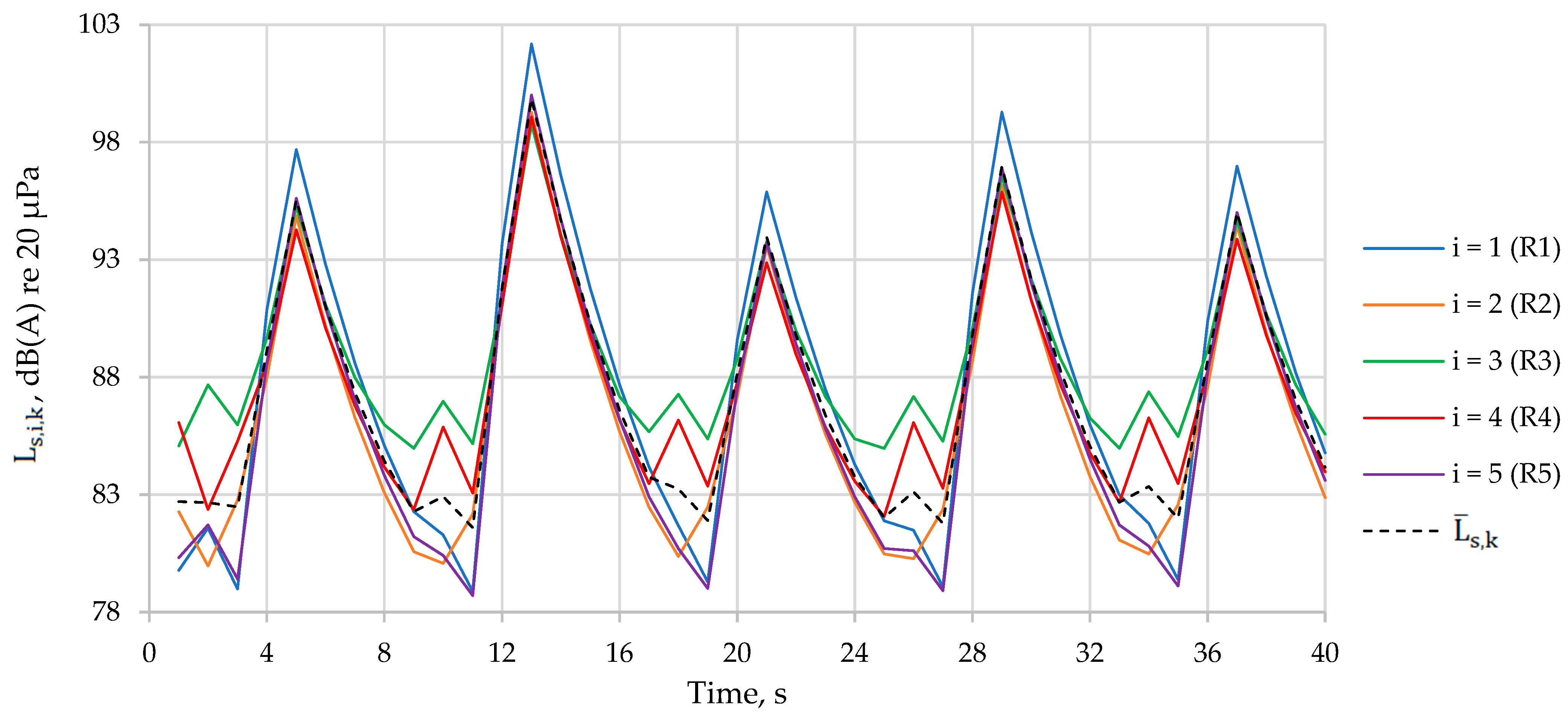
Figure 5 shows the individual back-calculated source SPL estimates (${\mathrm{L}}_{\mathrm{s},\mathrm{i},\mathrm{k}}$, Equation (7)) obtained from each of the five receivers separately, alongside their mean (${\overline{\mathrm{L}}}_{\mathrm{s},\mathrm{k}}$, Equation (8)). The five receiver-specific curves track each other closely and share the same impulsive pattern, which is the basis for treating their average as a single time-varying source estimate; the spread among the curves at a given time step provides a direct visual indication of the consistency error minimized in Equation (9).

Figure 5. Receiver-specific back-calculated source SPL estimates (${\mathrm{L}}_{\mathrm{s},\mathrm{i},\mathrm{k}}$) and their mean (${\overline{\mathrm{L}}}_{\mathrm{s},\mathrm{k}}$).

3.4. Reconstruction Consistency Check Results

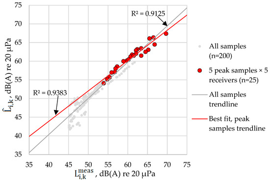
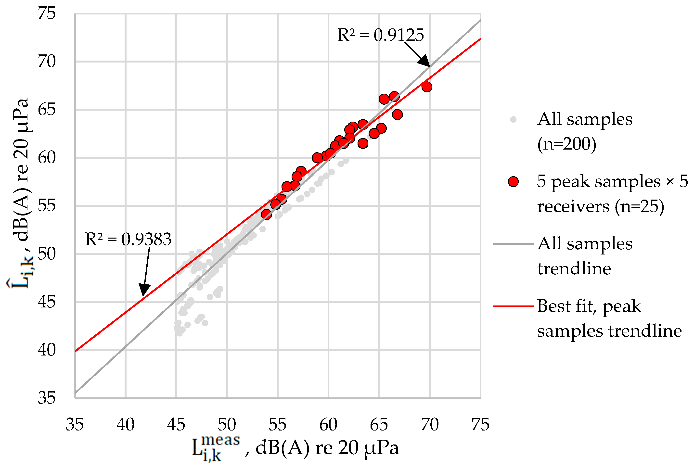
To check the internal consistency of the inverse model, predicted SPL values were computed at all five receiver positions using the estimated source coordinates and the calculated source SPL time series. The predicted and measured SPL values showed good agreement in magnitude (Figure 6). The temporal peaks were also reproduced through the time-dependent source SPL estimation.

Figure 6. Comparison of measured and predicted SPL values at the five receivers, showing both the full dataset ($\mathrm{n}$ = 200, ${\mathrm{R}}^2$ = 0.913) and the subset of five peak samples per receiver ($\mathrm{n}$ = 25, ${\mathrm{R}}^2$ = 0.939), which reduces the influence of within-pulse autocorrelation on the apparent correlation.

For the entire dataset (5 receivers × 40 time steps), the overall MAE was 1.3 dB(A), and the overall RMSE was 1.6 dB(A), indicating that the model reproduces the measured receiver levels with low residual error for such a simple geometrical spreading-based formulation. Because the same dataset was used both to estimate the source position and level and to compute these errors, this constitutes an in-sample consistency check rather than an independent validation of localization accuracy; no ground-truth source coordinates were available for direct comparison. The receiver-specific MAE values ranged from 1 dB(A) to 1.6 dB(A), while the RMSE values ranged from 1.4 dB(A) to 2.2 dB(A) (Table 2). As an additional check, restricting the comparison in Figure 6 to the five samples corresponding to each receiver’s dominant pulse peak ($\mathrm{n}$ = 25, rather than all 200 measured/predicted pairs) avoids inflating the apparent agreement through within-pulse autocorrelation. This subset yielded ${\mathrm{R}}^2$ = 0.939, slightly higher than ${\mathrm{R}}^2$ = 0.913 for the full dataset, indicating the model’s agreement with the measured data is not an artifact of closely spaced, autocorrelated samples within each pulse. The lowest MAE values were obtained for R5 (1.0 dB(A)) and R4 (1.0 dB(A)), while R3 recorded both the largest MAE (1.6 dB(A)) and the largest RMSE (2.2 dB(A)), consistent with its greater distance from the estimated source. Note that R5’s mean (bias) error (−1.0 dB(A)) was comparable in magnitude to R2’s (−1.0 dB(A)), both reflecting a small systematic underestimate rather than negligible bias, indicating that its low MAE reflects small random scatter rather than negligible systematic offset. This pattern is not fully monotonic with distance; however, R1, the closest receiver, also showed a comparatively large RMSE (1.8 dB(A)). This is plausible because near-field measurements are more sensitive to absolute coordinate and orientation errors (a fixed positioning uncertainty translates into a larger relative distance error at short range) and because interference between direct and ground-reflected paths is typically strongest close to the source. R3, conversely, is more likely to accumulate broadband propagation effects such as reflections and shielding over its longer path.

Table 2. Reconstruction consistency metrics for the predicted SPL values.

Receiver	${\mathbf{L}}_{\mathbf{e}\mathbf{q}}^{\mathbf{m}\mathbf{e}\mathbf{a}\mathbf{s}}$, dB(A) Re 20 µPa	${\widehat{\mathbf{L}}}_{\mathbf{i},\mathbf{k}}$, dB(A) Re 20 µPa	MAE, dB(A)	RMSE, dB(A)	Mean Error, dB(A)
R1	59.8	57.9	1.6	1.8	0.4
R2	55.9	56.7	1.1	1.4	−1.0
R3	50.6	50.6	1.6	2.2	1.5
R4	52.8	53.5	1.0	1.4	0.2
R5	56.7	56.9	1.0	1.4	−1.0
Overall	−	−	1.3	1.6	0.0

Individual receiver values are rounded to one decimal place for display. The Overall mean error is computed from the full unrounded residuals and is exactly zero by construction, since the source-level estimate at each time step is defined as the mean of the five receivers’ values.

A comparison of equivalent SPL values confirmed close agreement between measured and predicted data across all five receivers (Table 2). Despite its simplified formulation, the model reproduced the observed construction-noise field with low residual error.

3.5. Sensitivity and Uncertainty Analysis Results

Under receiver-coordinate uncertainty alone (${\mathsf{\sigma }}_{\mathrm{r}}$ = 3 m), the estimated source position had a standard deviation of 2.3 m in x and 2.6 m in y, with a 95% confidence region of semi-axes 4.5 m and 7.3 m and a 95th-percentile radial displacement of 6.1 m from the baseline estimate. Under SPL measurement uncertainty alone (${\mathsf{\sigma }}_{\mathrm{L}}$ = 1.5 dB), the position was less sensitive, with a standard deviation of 1.0 m in x and 1.2 m in y, a 95% confidence region of semi-axes 2.0 m and 3.1 m, and a 95th-percentile radial displacement of 2.6 m. The initial Monte Carlo formulation assumed a constant measurement-noise standard deviation (${\mathsf{\sigma }}_{\mathrm{L}}$ = 1.5 dB) across all SPL levels, which propagated into a nearly uniform sample-to-sample standard deviation in ${\mathrm{L}}_{\mathrm{s},\mathrm{k}}^{\ast }$ (0.6–0.7 dB) regardless of instantaneous signal level. Because low-level readings between pulses are closer to the ambient background level and therefore carry proportionally greater uncertainty about the source’s true contribution, a level-dependent measurement-uncertainty model was adopted instead: ${\mathsf{\sigma }}_{\mathrm{L}}\left(\mathrm{L}\right)={\mathsf{\sigma }}_{\mathrm{L},0}·(1+{10}^{-(\mathrm{L}-{\mathrm{L}}_{\mathrm{f}\mathrm{l}\mathrm{o}\mathrm{o}\mathrm{r}})/10)})$, where ${\mathsf{\sigma }}_{\mathrm{L},0}$ = 1.5 dB and ${\mathrm{L}}_{\mathrm{f}\mathrm{l}\mathrm{o}\mathrm{o}\mathrm{r}}$ = 45.1 dB(A) is the lowest SPL observed in the dataset, used as a proxy for the ambient/background floor. ${\mathrm{L}}_{\mathrm{f}\mathrm{l}\mathrm{o}\mathrm{o}\mathrm{r}}$ was set to the lowest SPL value observed in the dataset (45.1 dB(A), Table A1) as a pragmatic, data-derived proxy for the ambient/background level, rather than an independently measured background noise floor, which was not recorded separately during the 5 s event. Repeating the 1000-realization Monte Carlo perturbation with this level-dependent model yielded a sample-to-sample standard deviation ranging from 0.66 dB at the loudest instants to 1.25 dB at the quietest instants between pulses (Pearson correlation of −0.92 between mean receiver SPL and error-bar magnitude at each time step), consistent with expectations for signal-to-noise-driven uncertainty at low sound levels. Repeating this Monte Carlo with both receiver-coordinate uncertainty (${\mathsf{\sigma }}_{\mathrm{r}}$ = 3 m) and the level-dependent SPL uncertainty applied simultaneously gave a similar range (0.69–1.25 dB, versus 0.66–1.25 dB for SPL uncertainty alone) and a comparable correlation with signal level ($\mathrm{r}$ = −0.93), indicating that coordinate uncertainty contributes a modest, roughly time-independent addition on top of the level-dependent pattern rather than changing it materially. Combining both sources of uncertainty produced a 95% confidence region with semi-axes of approximately 5.1 m and 8.0 m and a 95th-percentile radial displacement of 6.6 m (Figure 3). These results indicate that the localization result is more sensitive to receiver-coordinate accuracy than to SPL measurement accuracy, and that the practically achievable positioning precision is on the order of several meters rather than centimeters, consistent with the rounding convention used elsewhere in this manuscript (Section 3.2).

The sensitivity of the source position to the assumed geometrical spreading exponent was more pronounced than the measurement-error sensitivity. Varying the exponent within a moderate range representative of near-free-field to mildly excess-attenuation conditions ($\mathrm{n}$ = 1.85–2.15) shifted the estimated source position by 1.5–1.6 m relative to the spherical spreading baseline ($\mathrm{n}$ = 2.0). Larger deviations, representative of substantially different propagation regimes ($\mathrm{n}$ = 1.5 or $\mathrm{n}$ = 3.0), shifted the estimate by approximately 6–8 m. This confirms that the spherical spreading assumption (Section 2.3) is an important, though not dominant, source of positional uncertainty, and that the coordinate- and SPL-driven uncertainty described above should be interpreted as conditional on this assumption being approximately correct.

3.6. Sensitivity to Source Position Across the Search Zone

Because a single field event cannot establish whether the method performs consistently across the search zone, a synthetic validation was performed within the same model framework: source positions spanning the zone, including its edges and corners, were used to generate synthetic receiver data (Equations (5) and (6), using the field-reconstructed source-level history as a representative impulsive pattern), perturbed with the same measurement uncertainty used in Section 3.5 (${\mathsf{\sigma }}_{\mathrm{L}}$ = 1.5 dB SPL, ${\mathsf{\sigma }}_{\mathrm{r}}$ = 3 m per coordinate; 40 Monte Carlo realizations per position). Table 3 summarizes the resulting localization error against the known synthetic source position.

Table 3. Localization error (m) for synthetic sources across the search zone, evaluated against the known synthetic source position used to generate each test case.

Position Category	Mean Error (95th Percentile)	Delay-Corrected Mean Error (95th Percentile)
Center	2.7 m (5.3 m)	2.6 m (5.3 m)
Edge midpoints (avg. of 4)	5.7 m (14.1 m)	4.6 m (9.1 m)
Corners (avg. of 4)	10.5 m (25.0 m)	6.7 m (14.2 m)

The objective function (Equations (7)–(9)) was also reformulated so that, for each candidate position, a receiver-specific propagation delay ${\mathsf{\tau }}_{\mathrm{i}}={\mathrm{r}}_{\mathrm{i}}/\mathrm{c}$ ($\mathrm{c}$ = 343 m/s) was computed, and the corresponding receiver’s time series was time-shifted before comparison. Formally, for each candidate position, the propagation delay is

$${\mathsf{\tau }}_{\mathrm{i}}({\mathrm{x}}_{\mathrm{s}},{\mathrm{y}}_{\mathrm{s}})={\mathrm{r}}_{\mathrm{i}}({\mathrm{x}}_{\mathrm{s}},{\mathrm{y}}_{\mathrm{s}})/\mathrm{c},\overline{\mathsf{\tau }}=(1/5){\mathsf{\Sigma }}_{\mathrm{i}}{\mathsf{\tau }}_{\mathrm{i}}$$

(18)

and each receiver’s realigned SPL value at nominal time t_k is obtained using one of three interpolation schemes: (a) linear interpolation in the decibel domain: ${\mathrm{L}}_{\mathrm{i}}^{\mathrm{s}\mathrm{h}\mathrm{i}\mathrm{f}\mathrm{t}\left({\mathrm{t}}_{\mathrm{k}}\right)}=\mathrm{I}\mathrm{n}\mathrm{t}\mathrm{e}\mathrm{r}\mathrm{p}\_\mathrm{d}\mathrm{B}\left[{\mathrm{L}}_{\mathrm{i}}^{\mathrm{m}\mathrm{e}\mathrm{a}\mathrm{s}}\right]({\mathrm{t}}_{\mathrm{k}}+{\mathsf{\tau }}_{\mathrm{i}}-\overline{\mathsf{\tau }})$; (b) linear interpolation in the linear-power domain: ${\mathrm{L}}_{\mathrm{i}}^{\mathrm{s}\mathrm{h}\mathrm{i}\mathrm{f}\mathrm{t}\left({\mathrm{t}}_{\mathrm{k}}\right)}=10·{\log }_{10}\left\{\mathrm{I}\mathrm{n}\mathrm{t}\mathrm{e}\mathrm{r}\mathrm{p}\_\mathrm{l}\mathrm{i}\mathrm{n}\left[{10}^{{\mathrm{L}}_{\mathrm{i}}^{\mathrm{m}\mathrm{e}\mathrm{a}\mathrm{s}}/10}\right]({\mathrm{t}}_{\mathrm{k}}+{\mathsf{\tau }}_{\mathrm{i}}-\overline{\mathsf{\tau }})\right\}$; (c) nearest-sample shifting:

$${\mathrm{L}}_{\mathrm{i}}^{\mathrm{s}\mathrm{h}\mathrm{i}\mathrm{f}\mathrm{t}\left({\mathrm{t}}_{\mathrm{k}}\right)}={\mathrm{L}}_{\mathrm{i}}^{\mathrm{m}\mathrm{e}\mathrm{a}\mathrm{s}}\left({\mathrm{t}}_{{\mathrm{k}}_{+}}\mathrm{r}\mathrm{o}\mathrm{u}\mathrm{n}\mathrm{d}\right(({\mathsf{\tau }}_{\mathrm{i}}-\overline{\mathsf{\tau }})/∆\mathrm{t}\left)\right),$$

(19)

where $∆\mathrm{t}$ = 0.125 s is the sampling interval. Equations (7)–(9) are then evaluated using ${\mathrm{L}}_{\mathrm{i}}^{\mathrm{s}\mathrm{h}\mathrm{i}\mathrm{f}\mathrm{t}}$ in place of ${\mathrm{L}}_{\mathrm{i}}^{\mathrm{m}\mathrm{e}\mathrm{a}\mathrm{s}}$.

Here ${\mathrm{r}}_{\mathrm{i}}({\mathrm{x}}_{\mathrm{s}},{\mathrm{y}}_{\mathrm{s}})$ denotes the distance from receiver i to the candidate position (${\mathrm{x}}_{\mathrm{s}},{\mathrm{y}}_{\mathrm{s}}$) currently being evaluated during the grid search, not the true, unknown source position, consistent with its use elsewhere in Equations (5)–(9).

Applied to the field dataset (Section 3.2), this delay-corrected inversion shifted the estimated source position by approximately 6.5 m from the baseline estimate and, compared with the independently surveyed ground-truth position (Section 3.2), had a localization error of 8.5 m—greater than the 2.3 m obtained for the uncorrected baseline estimate. The delay correction therefore did not improve, and in this case reduced, localization accuracy for the present event. This is consistent with the source position falling near the zone center, where propagation-delay differences are small. The synthetic sweep below (Table 3) was therefore repeated with the delay-corrected inversion to test whether the same holds at the zone edges.

Because the two farthest receivers (R3, R4) show secondary shoulders suggestive of multipath/echo arrivals (Figure 2), the inversion was repeated using only the three samples nearest each of the five dominant pulse peaks (15 of 40 samples), to test whether restricting the analysis to peak levels reduces the influence of echo contamination. Against the surveyed ground truth, this reduced-sample estimate had a localization error of 6.3 m, larger than the 2.3 m obtained using the full 40-sample series. This suggests that, for this dataset, the loss of averaging over more samples outweighs any reduction in multipath-related bias; the full time series was therefore retained as the primary analysis. Multipath contamination remains a plausible contributor to the larger residual errors at R3 and R4 (Table 2) and is noted as a limitation (Section 4).

Localization error increases three- to five-fold from the center to the edges and corners of the search zone, confirming that the single, centrally located field event reported in Section 3.2 is not representative of performance across the full search area. This synthetic evaluation is necessarily model-consistent, since the same propagation assumptions used in the inverse model also generate the test data; it demonstrates numerical identifiability under those assumptions rather than robustness to model mismatch (e.g., ground reflection, shielding, or non-spherical spreading) that may occur in real construction environments. The single field-validated result (Section 3.2, 2.3 m localization error) provides one data point of evidence under real, non-synthetic conditions, but broader model-mismatch robustness would require validation across multiple real sites and events, which was outside the scope of this study.

3.7. Out-of-Sample Cross-Validation

To address the in-sample nature of the reconstruction-consistency metrics reported in Section 3.4, a leave-one-receiver-out (LORO) cross-validation was performed. For each of the five receivers in turn, the source position and source-level history were re-estimated using only the remaining four receivers, and the held-out receiver’s measured SPL (data never used in that fit) was predicted from the resulting estimate. This is a genuinely out-of-sample test that does not require ground-truth source coordinates. The resulting out-of-sample MAE and RMSE were 3.1 dB(A) and 3.8 dB(A), respectively, compared with the in-sample values of 1.3 dB(A) and 1.7 dB(A) reported in Section 3.4. As expected, the out-of-sample error is higher, confirming that the in-sample metrics understate the error that would be obtained on genuinely independent data; the out-of-sample values reported here are a more representative estimate of the model’s SPL-reconstruction accuracy; the primary accuracy figure for the localization task itself is the 2.3 m spatial error against the surveyed ground-truth position (Section 3.2).

3.8. Comparison with Baseline Localization Methods

The proposed method was compared against two standard RSS-based baselines applied to the same dataset: weighted-centroid localization (receiver positions weighted by linear-domain received power) and RSS/path-loss least-squares localization (assuming a constant equivalent source level, Equation (6) with $\mathrm{n}$ = 2). Table 4 reports the reconstruction MAE/RMSE for each.

Table 4. Reconstruction accuracy of the proposed method versus baseline localization methods.

Method	MAE, dB(A)	RMSE, dB(A)	Localization Error vs. Ground-Truth, m
Proposed method (Section 2.4)	1.3	1.7	2.3
RSS/path-loss least-squares (constant source level)	1.3	1.9	5.8
Weighted centroid	1.7	2.1	11.3

The proposed method outperforms weighted centroid and is comparable to RSS least-squares on mean absolute reconstruction error, with a lower RMSE indicating fewer large errors. Evaluated against the independently surveyed ground-truth position (Section 3.2), the difference is much more pronounced: the proposed method’s localization error (2.3 m) is roughly 2.5 times lower than RSS least-squares (5.8 m) and 5 times lower than weighted centroid (11.3 m), despite the three methods showing comparable reconstruction MAE/RMSE—illustrating that reconstruction accuracy and true localization accuracy are not interchangeable metrics. Joint estimation of the path-loss exponent alongside source position, and joint localization assuming a constant (rather than time-varying) source level as a distinct baseline, were not implemented.

4. Discussion

The results show that synchronized SPL measurements from five spatially distributed receivers can be used to estimate both the position and the time-dependent acoustic strength of an active pile-driving source. The measured records exhibited five dominant peaks at approximately 1 s intervals, and these peaks occurred consistently across all receivers. This behavior agrees with the experimental observations of Imanov et al. [5], who found that pulsed sounds exhibit substantially greater short-term fluctuations and more pronounced peaks than steady or blended sounds. The present findings extend that observation from controlled propagation tests to an active construction site and demonstrate that the common temporal structure of an impulsive signal can be retained despite differences in receiver distance and local propagation conditions.

The spatial distribution of the measured levels was also physically consistent with the estimated source location. R1, R5, and R2, located 42.1–48.8 m from the estimated source, recorded higher equivalent SPL values than R4 and R3, located 70.6 and 98.5 m away, respectively. This confirms the general reduction in SPL with increasing source–receiver distance reported by Imanov et al. [5] and assumed in earlier construction-noise models [2,12,13,14]. Unlike those studies, however, the present model did not require the source coordinates to be known beforehand. Instead, the source was localized at [56.6, 113.8] m by identifying the point at which distance-corrected source-level estimates from all five receivers showed the greatest agreement. This inverse formulation therefore complements conventional construction-noise prediction approaches, which usually calculate receiver levels from predefined equipment positions.

The estimated equivalent source SPL was 90.4 dB(A) at the reference distance of 1 m, while the instantaneous estimates ranged from 81.6 to 99.9 dB(A). This range reflects the strongly non-stationary nature of pile driving and indicates that a single constant source value would not adequately describe the considered event. The use of an energy-based equivalent level is consistent with the treatment of temporally varying construction noise by Zhang and Pei [13]. It is also worth noting that the 0.125 s sampling interval used to resolve ${\mathrm{L}}_{\mathrm{s},\mathrm{k}}^{\ast }$ may be finer than physically meaningful for characterizing individual pile strikes: the observed fluctuations more plausibly reflect the presence or absence of a strike within each interval than a continuously varying source level. A per-strike sound exposure level (SEL), integrating the acoustic energy of each identified impulse over its own duration, may therefore be a more physically appropriate descriptor of single-strike source strength than the fixed-interval ${\mathrm{L}}_{\mathrm{s},\mathrm{k}}^{\ast }$ time series presented here, and is identified as a refinement for future work. Nevertheless, the estimated value at 1 m should be understood as a normalized source-strength indicator obtained by back-calculation, rather than as a direct measurement made physically 1 m from the pile. This interpretation is consistent with the caution raised by Ainslie et al. [7] regarding reference-distance source levels. Direct numerical comparison with the offshore pile-driving measurements of Bailey et al. [6] would be inappropriate because underwater and airborne propagation involve different reference pressures and transmission mechanisms; however, both studies demonstrate the value of multi-distance measurements for evaluating impulsive sources and propagation assumptions.

The overall MAE of 1.3 dB(A) and RMSE of 1.6 dB(A) indicate that the simplified model reproduces the measured receiver levels with low residual error under the present in-sample consistency check (Section 3.4). Because this study is based on a single 5 s event at one construction site, evaluated in-sample rather than against an independent test dataset, these values are not directly comparable to prediction errors reported for other construction-noise models, which differ in equipment, measurement duration, environmental conditions, and, most importantly, validation procedure. For context only, Manatakis and Skarlatos [12] reported a standard error of approximately 2 dB(A), Hong et al. [14] obtained a 2.76 dB(A) difference between predicted and measured levels, Lee et al. [19] reported RMSE values of 2.62 and 2.70 dB, and Ooi et al. [21] reported an average absolute difference below 1.2 dB(A); these figures indicate only the general order of magnitude of prediction errors reported elsewhere in the construction-noise literature, not a like-for-like benchmark. A rigorous comparison would require applying the present method and the cited approaches to a common, independently validated dataset, which is beyond the scope of this study.

It should be emphasized that the low MAE and RMSE reported above demonstrate internal consistency, that is, agreement between the measured receiver levels and those reconstructed from the estimated source position and source-level history, rather than independently validated localization accuracy. The as-driven pile position was independently surveyed (Section 3.2), giving a true localization error of 2.3 m for the estimate at [56.6, 113.8] m, within the range anticipated by the Monte Carlo sensitivity analysis below. The Monte Carlo sensitivity analysis in Section 3.5 characterizes how the estimate would be expected to vary under plausible input errors, but this is conditional on the model’s assumptions (Section 2.7) and does not substitute for comparison against a directly measured source position. A leave-one-receiver-out cross-validation (Section 3.7), which does not require ground-truth coordinates, gives a more representative out-of-sample error (MAE 3.1 dB(A), RMSE 3.8 dB(A)) than the in-sample values above.

The receiver-specific errors provide insight into the limitations of the simplified propagation assumption. R3, the farthest receiver, had the largest RMSE of 2.2 dB(A) and a positive mean error, whereas lower errors were obtained at R4 and R5. Outdoor sound propagation is affected by ground impedance, direct-reflected-wave interference, atmospheric gradients, turbulence, diffraction, and screening [8,9]. Harmonoise explicitly separates geometrical divergence from atmospheric absorption, ground effects, diffraction, refraction, and turbulence-related excess attenuation [10]. These mechanisms were not modelled individually in the present study and were absorbed into the residual error. The larger deviation at R3 may therefore reflect the accumulation of unmodelled propagation effects over its longer path, although this interpretation cannot be confirmed without frequency-resolved, meteorological, and site-obstruction data.

A further limitation concerns the temporal alignment assumed in Equations (7)–(9). The model treats the SPL values recorded at the same time index $\mathrm{k}$ across all five receivers as corresponding to the same source event, effectively assuming instantaneous propagation. However, sound travels at approximately 343 m/s, and the estimated source-to-receiver distances ranged from 42.1 m (R1) to 98.5 m (R3), a difference of about 56 m. This corresponds to a propagation-time difference of roughly 0.16 s, exceeding one 0.125 s sampling interval. Consequently, the SPL value recorded at a given $\mathrm{k}$ at the farthest receiver may in fact correspond to an acoustic event emitted slightly earlier than the one captured at the same $\mathrm{k}$ by the nearest receiver. This effect is distinct from the recording synchronization described in Section 2.1: it arises from the physical travel time of sound across the search zone and would persist even with perfectly synchronized recordings. We also note that although the source-strength estimation in Section 2.4 does not require the phase-level timing precision needed by time-of-arrival localization methods, consistent with the RSS-based framing discussed in the Introduction, the coarser sample-level alignment addressed here remains relevant because, for acoustic signals propagating over tens to hundreds of meters, propagation delay can be comparable to the sampling interval itself. Since individual pile-driving pulses persisted over several consecutive samples in the measured records (Table A1), a misalignment on the order of one sample is expected to partially blur, rather than eliminate, the correspondence between simultaneous source events and receiver readings, and is unlikely to account for the full magnitude of the residual errors reported in Table 2. This delay correction was implemented and tested directly (Section 3.6).

The model also neglects the vertical offset between the pile-driving impact point and the ground-level receiver positions, treating the geometry as coplanar (Section 2.7). For representative pile-driving rig heights of approximately 5–20 m and the horizontal source-to-receiver distances obtained in this study (42.1–98.5 m), the three-dimensional distance differs from the horizontal distance used in the model by at most about 0.9 dB(A) at the closest receiver (R1) and by less than 0.1 dB(A) at the farthest receiver (R3), based on the spherical spreading relationship in Equation (6). This bias is smaller than the overall MAE of 1.3 dB(A) obtained in the reconstruction consistency check (Table 2), suggesting that the horizontal-plane approximation is unlikely to be a dominant source of error for the receiver distances considered here, although it would become more significant for receivers positioned much closer to the source.

An additional simplification concerns the exclusive treatment of the source as an airborne point emitter. In practice, pile driving transfers substantial vibration energy directly into the ground, which can propagate as ground-borne waves and re-radiate as airborne sound near each receiver, particularly for receivers close to the ground surface [36]. This mechanism is not represented by the geometrical spreading term in Equation (6) and is therefore absorbed into the residual error ${\mathsf{\epsilon }}_{\mathrm{i},\mathrm{k}}$ together with reflection, shielding, and scattering effects. Because ground-borne re-radiation depends on local soil properties and receiver coupling rather than on source-receiver distance alone, it may contribute to the site-specific component of the residual error observed at individual receivers (Table 2); separating this contribution would require dedicated vibration measurements, which were outside the scope of the present acoustic field campaign.

Finally, the inverse formulation in Equations (7)–(10) is derived under the assumption of a single dominant source. Because the back-calculated source level in Equation (7) is sensitive to small changes in received SPL, particularly at larger distances, the simultaneous presence of additional sound sources or strong, time-delayed echoes from nearby structures, which effectively act as additional apparent sources at a given sampling instant, could substantially degrade the localization result. This restricts the direct applicability of the method to relatively open construction sites with a single dominant impulsive source, away from other concurrent construction activity or dense urban surroundings; extending the approach to multi-source or strongly reverberant environments would require explicit source separation or reflection modelling, which is beyond the scope of the present single-source formulation.

With the independently surveyed ground-truth position now available (Section 3.2), it is useful to state explicitly what would constitute an acceptable result for the intended application. For construction-site noise source attribution and rapid GIS-based monitoring, a positioning precision on the order of several meters, sufficient to associate a source estimate with a specific piece of equipment or work area rather than an exact ground point, is generally adequate; sub-meter precision is not required for this purpose. The 95% confidence region obtained in Section 3.5 (semi-axes of approximately 5–8 m under combined coordinate and measurement uncertainty) falls within this range relative to the scale of the search zone (104.4 m × 182.16 m), and is consistent with the 2.3 m localization error actually obtained against the surveyed ground truth.

Compared with established localization techniques, the principal advantage of the proposed approach is its operational simplicity. Conventional beamforming requires multi-channel waveform or phase information, and its resolution depends on array geometry, aperture, and frequency [24]. Time-reversal localization requires a numerical representation of the surrounding propagation environment [25], while reflection-aware localization benefits from reconstructed geometry and explicit reflected paths [26]. Finite-element inverse schemes and sparse reverse beamforming can provide more detailed source reconstructions but require transfer functions, waveform data, or regularization [29,30]. In contrast, the present method uses synchronized scalar SPL values, known receiver coordinates, and a simple objective function. This makes it suitable for practical sound level meters that cannot supply the waveform information required by array-processing methods, although it cannot provide their spatial resolution or multiple-source separation capability.

The results also have practical implications for construction-noise management. Planning and optimization methods developed by Kwon et al. [15], Ning et al. [16], Kantová [17], and Baek et al. [18] generally require information about source or equipment locations. The proposed inverse procedure could supply such information when an active source is uncertain or changes during construction. It could also support the sensor- and GIS-based monitoring concept proposed in [22] and address the need for affordable and adaptable monitoring solutions identified in [33].

The study is limited to one 5 s measurement event, one construction site, five receivers, and one assumed stationary point source. The actual source coordinates were independently surveyed for this one event (Section 3.2); prediction errors at the receivers validate sound-field reconstruction, while the 2.3 m localization error quantifies positional accuracy for this event specifically; repeated events and sites were not surveyed. Manual extraction of the UT352 readings may also introduce timing and transcription uncertainty. Future work should validate the estimated position against surveyed ground-truth source coordinates, repeat measurements over longer periods and different pile-driving stages, and quantify sensitivity to receiver number and placement. It should be emphasized that incorporating meteorological, ground, barrier, and reflection corrections would depart from the deliberately simple, low-cost formulation prioritized in this study and would more closely resemble comprehensive engineering propagation models, such as Harmonoise [10] or the ISO 9613-2 and ANSI/ASA S1.26 standards [20,35], rather than a direct extension of the present inverse method. Development more consistent with the current approach, such as formal uncertainty quantification, together with integration into an automated real-time sensor and GIS platform, is identified as a more immediate next step; frequency-band information and multiple-source handling would similarly require a substantially different modelling framework. This scope reflects a genuine constraint on the present study rather than an oversight; broadening it to multiple sites, events, receiver configurations, and source types was not undertaken and is identified explicitly, rather than implicitly, as necessary future work before the method’s general applicability can be established.

5. Conclusions

This study developed and field-tested a transparent inverse acoustic model for jointly estimating the location and time-dependent sound pressure level of an unknown pile-driving source using synchronized measurements from five spatially distributed receivers. Applied to a 5 s construction-site event comprising 40 measurements per receiver, the model localized the source at [56.6, 113.8] m, with a 95% confidence region of approximately 5–8 m under combined coordinate and measurement uncertainty, and estimated an equivalent source SPL of 90.4 dB(A) at the reference distance of 1 m. The reconstructed source history preserved the impulsive and quasi-periodic character of pile driving, with peak values reaching 99.9 dB(A). Agreement between measured and predicted receiver levels was satisfactory, yielding an overall MAE of 1.3 dB(A) and RMSE of 1.6 dB(A); these values reflect internal consistency between measured and reconstructed receiver levels. Independently surveyed ground-truth coordinates for the pile gave a true localization error of 2.3 m for the estimated position. These findings demonstrate that useful construction-noise source localization and strength estimation can be achieved from scalar SPL measurements without microphone-array waveform data, complex environmental simulations, or extensive training datasets. The method therefore provides a practical basis for rapid field assessment and future integration into automated sensor- and GIS-based monitoring systems. Nevertheless, broader validation should include independently surveyed source coordinates at additional sites and events, longer measurements, different receiver arrangements, multiple construction sites, and corrections for meteorological conditions, ground effects, barriers, reflections, propagation delay across the receiver network, and multiple or moving sources.

References

- Ballesteros, M.J.; Fernández, M.D.; Quintana, S.; Ballesteros, J.A.; González, I. Noise Emission Evolution on Construction Sites. Measurement for Controlling and Assessing Its Impact on the People and on the Environment. Build. Environ. 2010, 45, 711–717. [Google Scholar] [CrossRef] [Scilit]
- Gilchrist, A.; Allouche, E.N.; Cowan, D. Prediction and Mitigation of Construction Noise in an Urban Environment. Can. J. Civ. Eng. 2003, 30, 659–672. [Google Scholar] [CrossRef] [Scilit]
- Zou, C.; Zhu, R.; Tao, Z.; Ouyang, D.; Chen, Y. Evaluation of Building Construction-Induced Noise and Vibration Impact on Residents. Sustainability 2020, 12, 1579. [Google Scholar] [CrossRef] [Scilit]
- Zhang, J.; Huang, J.; Wu, Z.; Li, Z. Construction Noise Reduction Research on Rail Transit Projects: A Case Study in China. Buildings 2024, 14, 1678. [Google Scholar] [CrossRef] [Scilit]
- Imanov, A.; Kozhas, A.; Mukhamejanova, A.; Nazarova, A.; Kazhimkanuly, D. Experimental Study of Sound Wave Propagation Patterns. Technobius 2024, 4, 0057. [Google Scholar] [CrossRef] [Scilit]
- Bailey, H.; Senior, B.; Simmons, D.; Rusin, J.; Picken, G.; Thompson, P.M. Assessing Underwater Noise Levels during Pile-Driving at an Offshore Windfarm and Its Potential Effects on Marine Mammals. Mar. Pollut. Bull. 2010, 60, 888–897. [Google Scholar] [CrossRef] [Scilit] [PubMed]
- Ainslie, M.A.; De Jong, C.A.F.; Robinson, S.P.; Lepper, P.A. What Is the Source Level of Pile-Driving Noise in Water? In The Effects of Noise on Aquatic Life; Advances in Experimental Medicine and Biology; Springer: New York, NY, USA, 2012; Volume 730, pp. 445–448. [Google Scholar]
- Attenborough, K. Review of Ground Effects on Outdoor Sound Propagation from Continuous Broadband Sources. Appl. Acoust. 1988, 24, 289–319. [Google Scholar] [CrossRef] [Scilit]
- Embleton, T.F.W. Tutorial on Sound Propagation Outdoors. J. Acoust. Soc. Am. 1996, 100, 31–48. [Google Scholar] [CrossRef] [Scilit]
- Salomons, E.; Van Maercke, D.; Defrance, J.; De Roo, F. The Harmonoise Sound Propagation Model. Acta Acust. United Acust. 2011, 97, 62–74. [Google Scholar] [CrossRef] [Scilit]
- Manatakis, E.K. A New Methodological Trial on Statistical Analysis of Construction Equipment Noise. Appl. Acoust. 2000, 59, 67–76. [Google Scholar] [CrossRef] [Scilit]
- Manatakis, E.; Skarlatos, D. A Statistical Model for Evaluation and Prediction of the Noise Exposure in a Construction Equipment Area. Appl. Acoust. 2002, 63, 759–773. [Google Scholar] [CrossRef] [Scilit]
- Zhang, H.; Pei, Y. Simulation-Based Prediction of Equivalent Continuous Noises during Construction Processes. Int. J. Environ. Res. Public Health 2016, 13, 818. [Google Scholar] [CrossRef] [Scilit] [PubMed]
- Hong, T.; Ji, C.; Park, J.; Leigh, S.-B.; Seo, D. Prediction of Environmental Costs of Construction Noise and Vibration at the Preconstruction Phase. J. Manag. Eng. 2015, 31, 04014079. [Google Scholar] [CrossRef] [Scilit]
- Kwon, N.; Park, M.; Lee, H.-S.; Ahn, J.; Kim, S. Construction Noise Prediction Model Based on Case-Based Reasoning in the Preconstruction Phase. J. Constr. Eng. Manag. 2017, 143, 04017008. [Google Scholar] [CrossRef] [Scilit]
- Ning, X.; Qi, J.; Wu, C.; Wang, W. Reducing Noise Pollution by Planning Construction Site Layout via a Multi-Objective Optimization Model. J. Clean. Prod. 2019, 222, 218–230. [Google Scholar] [CrossRef] [Scilit]
- Kantová, R. Evaluation of Construction Site Noise to Allow the Optimisation of Construction Processes and Construction Machinery Selection. Appl. Sci. 2021, 11, 4389. [Google Scholar] [CrossRef] [Scilit]
- Baek, H.; Jung, S.; Hong, J.; Hong, T. Simulation-Based Framework for Optimal Construction Equipment Allocation Considering Construction Noise Emissions. J. Asian Archit. Build. Eng. 2023, 22, 2959–2976. [Google Scholar] [CrossRef] [Scilit]
- Lee, G.; Moon, S.; Hwang, J.; Chi, S. Development of a Real-Time Noise Estimation Model for Construction Sites. Adv. Eng. Inform. 2023, 58, 102133. [Google Scholar] [CrossRef] [Scilit]
- ISO 9613-2:2024; Acoustics—Attenuation of Sound During Propagation Outdoors Part 2: Engineering Method for the Prediction of Sound Pressure Levels Outdoors. International Organization for Standardization: Geneva, Switzerland, 2024.
- Ooi, W.C.; Lim, M.H.; Lee, Y.L. Development of Stochastic Deep Learning Model for the Prediction of Construction Noise. Ain Shams Eng. J. 2024, 15, 102592. [Google Scholar] [CrossRef] [Scilit]
- Utepov, Y.; Imanov, A. Conceptual Model of Noise Monitoring System for Construction Projects in Cramped Conditions, Based on Sensors and GIS. Technobius 2022, 2, 0025. [Google Scholar] [CrossRef] [Scilit]
- Utepov, Y.; Imanov, A.; Mukhamejanova, A.; Kozhas, A.; Akhazhanov, S. Review of Existing Solutions for Vibroacoustic Monitoring of Construction Sites. Eurasian J. Appl. Eng. Technol. 2024, 147, 61–76. [Google Scholar] [CrossRef] [Scilit]
- Chiariotti, P.; Martarelli, M.; Castellini, P. Acoustic Beamforming for Noise Source Localization Reviews, Methodology and Applications. Mech. Syst. Signal Process. 2019, 120, 422–448. [Google Scholar] [CrossRef] [Scilit]
- Albert, D.G.; Liu, L.; Moran, M.L. Time Reversal Processing for Source Location in an Urban Environment. J. Acoust. Soc. Am. 2005, 118, 616–619. [Google Scholar] [CrossRef] [Scilit]
- An, I.; Son, M.; Manocha, D.; Yoon, S.-E. Reflection-Aware Sound Source Localization. In Proceedings of the 2018 IEEE International Conference on Robotics and Automation (ICRA); IEEE: Brisbane, QLD, Australia, 2018; pp. 66–73. [Google Scholar]
- Cobos, M.; Antonacci, F.; Alexandridis, A.; Mouchtaris, A.; Lee, B. A Survey of Sound Source Localization Methods in Wireless Acoustic Sensor Networks. Wirel. Commun. Mob. Comput. 2017, 2017, 3956282. [Google Scholar] [CrossRef] [Scilit]
- Chang, S.; Li, Y.; He, Y.; Wu, Y. RSS-Based Target Localization in Underwater Acoustic Sensor Networks via Convex Relaxation. Sensors 2019, 19, 2323. [Google Scholar] [CrossRef] [Scilit] [PubMed]
- Gombots, S.; Nowak, J.; Kaltenbacher, M. Sound Source Localization State of the Art and New Inverse Scheme. E I Elektrotechnik Und Informationstechnik 2021, 138, 229–243. [Google Scholar] [CrossRef] [Scilit]
- Sun, C.; Liu, Y. Spherical Reverse Beamforming for Sound Source Localization Based on the Inverse Method. Sensors 2019, 19, 2618. [Google Scholar] [CrossRef] [Scilit] [PubMed]
- Nelson, P.A.; Yoon, S.H. Estimation of Acoustic Source Strength by Inverse Methods: Part i, Conditioning of the Inverse Problem. J. Sound Vib. 2000, 233, 639–664. [Google Scholar] [CrossRef] [Scilit]
- Yoon, S.H.; Nelson, P.A. Estimation of Acoustic Source Strength by Inverse Methods: Part II, Experimental Investigation of Methods for Choosing Regularization Parameters. J. Sound Vib. 2000, 233, 665–701. [Google Scholar] [CrossRef] [Scilit]
- Utepov, Y.; Mukhamejanova, A.; Nazarova, A.; Aniskin, A.; Kozhas, A.; Imanov, A. Geospatial Visualization of Logarithmic Attenuation of Pile-Driving Noise Based on Field Measurements. Eng. Sci. 2025, 35, 1562. [Google Scholar] [CrossRef] [Scilit]
- Skudrzyk, E. Spherical Waves, Sources, and Multipoles. In The Foundations of Acoustics; Springer: Vienna, Austria, 1971; pp. 344–377. [Google Scholar]
- ANSI/ASA S1.26-2014; Methods for Calculation of the Absorption of Sound by the Atmosphere. Acoustical Society of America: Melville, NY, USA, 2014.
- Colaço, A.; Alves Costa, P.; Mont’Alverne Parente, C.; Silva Cardoso, A. Ground-Borne Noise and Vibrations in Buildings Induced by Pile Driving: An Integrated Approach. Appl. Acoust. 2021, 179, 108059. [Google Scholar] [CrossRef] [Scilit]
Disclaimer/Publisher’s Note: The statements, opinions and data contained in all publications are solely those of the individual author(s) and contributor(s) and not of MDPI and/or the editor(s). MDPI and/or the editor(s) disclaim responsibility for any injury to people or property resulting from any ideas, methods, instructions or products referred to in the content. |
© 2026 by the authors. Licensee MDPI, Basel, Switzerland. This article is an open access article distributed under the terms and conditions of the Creative Commons Attribution (CC BY) license.