


Abstract
Optical ground wire (OPGW) cables are subjected to extreme electromagnetic stresses from lightning and short circuits. Existing models have three main limitations: (i) they assume uniform current distribution, (ii) they use constant material properties, and (iii) they do not couple the electromagnetic, thermal, and mechanical domains. This paper proposes a coupled multiphysics model that incorporates non-uniform current distribution with dependent on the magnetic field, temperature-dependent properties, and differentiated failure criteria. The model was implemented in COMSOL Multiphysics and was validated against experimental short-circuit tests (15–30 kA) conducted at the HPT-Laboratory (FEC). For the lightning scenario (10/350 μs impulse), the model predictions were compared with experimental results reported in the literature, showing good agreement in temperature rise and damage patterns. Results show that including a non-uniform current distribution modifies the predicted maximum temperature by 15.8% and shifts its location from the center to the outer aluminum layers. The model reproduces the experimental temperature with an RMSE of <7 °C and a relative error of <8%. A combined failure criterion (thermal + mechanical) predicts strand breakage with 89.2% accuracy, outperforming the purely thermal (72.5%) and mechanical (78.3%) criteria. Specific and curves were generated for two commercial OPGW cable configurations (Manufacturer A and Manufacturer B), with capacities at 500 ms of 128 kA2s and 98 kA2s, respectively. The proposed model provides a useful tool for protection selection and coordination in transmission lines with OPGW cables.
1. Introduction
Optical ground wire (OPGW) cables are critical components in high-voltage transmission infrastructure [1,2]. Failures in OPGW cables represent between 12% and 18% of unplanned outages in transmission systems above 200 kV [3]. In Mexico, the Federal Electricity Commission (FEC) recorded more than 800 failure events between 2015 and 2023, with an average repair cost of USD 42,000 per incident [4].
Recent advances in fault detection for high-voltage cables have emphasized the need for accurate transient models to enable proper protection coordination [5]. However, available models and design standards—including those based on IEEE 738 [6] and IEC 60794 [7]—incorporate simplifications that limit their predictive accuracy:
- Uniform current distribution is assumed across all conductive layers, neglecting the skin effect and the presence of magnetic materials.
- Material properties are treated as constant, ignoring their dependence on temperature and magnetic field.
- The electromagnetic, thermal, and mechanical domains are solved in a decoupled manner, thereby missing the bidirectional interactions that occur during transient events.
These limitations have been partially addressed in recent studies [2,8,9,10,11], but a comprehensive coupled model that integrates non-uniform current distribution, temperature-dependent properties, and multiphysics coupling has not yet been reported in the literature. This gap is particularly critical for OPGW cables, where the combination of high magnetic permeability in steel layers, the relatively low melting temperature of aluminum, and the presence of an optical core creates a complex multiphysics problem that cannot be adequately captured by simplified approaches.
To address this gap, this work proposes a coupled electro-thermo-mechanical (ETM) model that incorporates:
- Non-uniform current distribution with dependent on the magnetic field and dependent on temperature.
- Temperature-dependent thermal and mechanical properties.
- Bidirectional coupling between the electromagnetic and thermal domains, and sequential coupling with the mechanical domain.
- Differentiated failure criteria (thermal, mechanical, and combined) to predict strand breakage.
The model was validated against experimental short-circuit tests (15–30 kA) conducted at the HPT-Laboratory (FEC). For the lightning scenario (10/350 μs impulse), direct experimental validation is not available in this study; instead, the model predictions were compared with experimental results reported in the literature [8,9]. The model reproduces the temperature and damage patterns reported in those studies within acceptable error bounds, although direct experimental verification remains a subject for future work. This distinction is important and is addressed again in the discussion of model limitations. The main research questions addressed in this work are:
- RQ 1: How and to what extent does the temperature field change when a non-uniform current distribution is incorporated?
- RQ 2: Which combination of thermal and mechanical criteria best predicts strand breakage?
- RQ 3: Can the thermo-mechanical state of the optical core be correlated with the increase in attenuation at 1550 nm?
The remainder of this paper is organized as follows. Section 2 presents the theoretical framework, including a description of the OPGW cable structure and material properties. Section 3 describes the mathematical model and the coupling strategy. Section 4 defines the excitation waveforms (lightning and short-circuit). Section 5 outlines the numerical implementation. Section 6 presents the results, including current and temperature distribution, comparison with uniform models, experimental validation, mechanical response, and design curves. Section 7 discusses the findings in the context of the research questions.
2. Theoretical Framework
This section presents the fundamental concepts and background needed to understand the proposed coupled model. First, the structure and material composition of OPGW cables are described. Next, the electromagnetic, thermal, and mechanical models reported in the literature are briefly discussed, highlighting their limitations and the need for a coupled approach.
2.1. OPGW Cable Structure and Composition
A typical OPGW cable consists of concentric layers that perform three functions: electrical (lightning and short-circuit current conduction), mechanical (tension support), and optical (data transmission). Figure 1 shows the idealized cross-section of the cable, while Figure 2 presents a simplified representation of its composition.
Figure 1.
(a) Optical Core Diagram Structure: Shows a cross-section of the central core. Elements: It is composed of four concentric layers. 1 Optical fiber (SiO2): The innermost layer, represented by multiple dots, has a radius (r) less than or equal to 0.5 mm. 2 Polymer coating: The next layer, between 0.5 mm and 0.8 mm thick. 3 Filling gel: The subsequent layer, with a thickness between 0.8 mm and 1.2 mm. 4 Steel tube (AISI 304): The outermost layer of this section, between 1.2 mm and 4.5 mm thick. (b) OPGW CABLE Diagram Structure: Shows a complete cross-section of the cable with an external diameter (∅) of 20 mm. Elements: It’s formed by six concentric layers. Optical Core: Layers 1 through 3 constitute the central core. Steel tube + ACS: Layers 4 and 5, where the steel tube encloses ACS wires. Al + ACS: Layers 5 and 6, where aluminum wires (AA1350) and ACS wires are present. 5 ACS wires: The 5th layer, composed of multiple wires with diameters between 4.5 mm and 7.5 mm. A text box highlights that ACS has a dual role of conduction and strength. 6 Aluminum wires (AA1350): The outermost layer (6th), with a diameter between 7.5 mm and 10 mm. ELECTRICAL (fault current): A text box in the upper right mentions that the skin effect concentrates the fault current in the outer layers (5–6), leading to non-uniform heating and hot spots. MECHANICAL (tensile load) and OPTICAL (data link): Other text boxes with arrows indicate the different functionalities of the cable. The material properties are summarized in Table 1.
Figure 2.
Simplified representation of the OPGW cable composition, emphasizing the material hierarchy: dielectric core (fiber + coating + gel), intermediate metallic barrier (stainless steel tube), and outer conductive layers (ACS and aluminum). The material properties are summarized in Table 1.
The concentric arrangement shown in Figure 1 plays a fundamental role because it determines the current distribution resulting from the skin and proximity effects. The outer metallic layers (layers 5 and 6) concentrate most of the current under transient conditions, while the optical core (layers 1 to 4) is partially shielded from electromagnetic fields by the steel tube.
Figure 2 emphasizes the material arrangement. This hierarchy is particularly relevant for the electromagnetic-thermal coupling, because steel exhibits high magnetic permeability () which influences the skin depth in adjacent layers, while aluminum has high electrical conductivity and a relatively low melting temperature.
The six radial layers and their main functions are:
- Layer 1 (optical fiber, SiO2): optical transmission medium at 1550 nm.
- Layer 2 (polymer coating, acrylate/PBT): primary mechanical protection of the fiber.
- Layer 3 (thixotropic filling gel): moisture blocking and mechanical damping.
- Layer 4 (stainless steel tube AISI 304): hermetic barrier and structural rigidity.
- Layer 5 (ACS wires, aluminum-clad steel): conductive layer and mechanical resistance.
- Layer 6 (aluminum wires AA 1350-H19): outer layer of high conductivity.
2.2. Material Properties
Table 1 summarizes the thermal, electrical, and mechanical properties of the materials used in the OPGW cable. These properties are temperature-dependent in the proposed model, except where noted.
Table 1.
Thermal, electrical, and mechanical properties of OPGW cable materials.
The material properties listed in Table 1 are applied to the proposed model. The following subsections present the mathematical expressions used for each material property, along with the rationale for using literature values.
2.2.1. Justification for Literature-Based Properties
The temperature-dependent material properties used in this work were taken from the literature and standardized material databases (ASM International and IEEE Standard 738-2012) [6] rather than measured directly from the tested cable. This approach was adopted for the following reasons:
- Non-destructive testing requirement: The tested cable is a commercial OPGW product, and destructive testing for material property extraction (e.g., tensile testing at elevated temperatures, thermal diffusivity measurements) would compromise its structural integrity and render it unsuitable for subsequent electrical testing.
- Standard industrial materials: The materials used in the cable—AA 1350-H19 aluminum, AISI 304 stainless steel, ACS steel, and polymer coatings—are standard industrial materials with well-established temperature-dependent properties extensively documented in the literature [6,12,13].
- Peer-reviewed sources: The literature values are derived from peer-reviewed sources and standardized material databases, ensuring their reliability and traceability.
- Indirect validation: The model predictions validated against experimental short-circuit tests (Section 5.9) indirectly confirm the adequacy of the literature-based material properties for the temperature range encountered in this study (20–300 °C).
2.2.2. Constitutive Equations for Material Properties
The following expressions are used for the temperature-dependent properties of the main metallic materials:
Electrical Conductivity of Aluminum (AA 1350-H19):
where S/m, °C−1, and °C−2, valid for .
Thermal Conductivity of Aluminum:
where W/(m·K), °C−1, and °C−2.
Specific Heat Capacity of Aluminum:
where J/(kg·K), °C−1, and °C−2.
Magnetic Permeability of ACS Steel:
The relative magnetic permeability of ACS steel depends on both the magnetic field intensity and temperature:
where is the maximum permeability at temperature T, and is the saturation field. At , and A/m. The temperature dependence is modeled as .
Electrical Conductivity of AISI 304 Stainless Steel:
where S/m, °C−1, and °C−2.
These expressions are based on ASM International (2023) and IEEE Standard 738-2012, with coefficients fitted to the temperature range 20–300 °C.
2.3. Electromagnetic Models
Current distribution in multilayer conductors is determined by the skin depth, defined as:
where is the angular frequency, is the magnetic permeability, and is the electrical conductivity. In OPGW cables with steel layers () and aluminum (), the skin depth differs significantly between layers, resulting in a markedly non-uniform current distribution [8]. This non-uniformity is often neglected in standard models based on IEEE 738 [6], which assume uniform heat generation.
2.4. Thermal Models
The IEEE 738 standard [6] provides thermal models for bare overhead conductors under steady-state and transient conditions. Dmitriev and González [1] used this approach for OPGW cables, although they assumed uniform heat generation and constant properties. More recently, finite element analysis has been applied to analyze the transient thermal response of electrical cables under fault conditions [14]. However, these studies typically treat the electromagnetic and thermal domains separately, neglecting the bidirectional coupling that occurs during transient events.
2.5. Mechanical Models
Stresses in OPGW cables arise from three simultaneous mechanisms [9]:
- Differential thermal expansion: Different materials (aluminum vs steel) have different coefficients of thermal expansion, generating interfacial stresses during heating and cooling.
- Electromagnetic forces: The interaction of current J with the induced magnetic field B generates Lorentz forces, which are maximum in regions of high current density.
- Mechanical service tension: OPGW cables are typically installed with a service tension of 15% to 25% of their breaking load.
Most existing mechanical models consider only the service tension [6], neglecting the transient stresses induced by thermal expansion and electromagnetic forces during fault events.
2.6. Experimental Background
Short-circuit tests at 15–30 kA have demonstrated surface temperatures of up to 287 °C, according to technical reports from the High-Power-Testing-Laboratory (HPTL) of FEC [4]. Cai et al. [9] documented that failure initiates in the outer layers, where current density is highest due to the skin effect. These experimental observations motivate the need for a model that captures non-uniform current distribution and its thermal and mechanical consequences.
2.7. Summary of Research Gaps
Based on the literature review, the following research gaps are identified:
- Current distribution is assumed uniform in most standards and models, despite the presence of magnetic materials and transient currents.
- Material properties are treated as constant, ignoring temperature dependence and field-dependent permeability.
- The electromagnetic, thermal, and mechanical domains are solved in a decoupled manner, thereby missing the interactions that occur during transient events.
- Failure criteria are typically based on a single domain (thermal or mechanical), leading to inaccurate predictions of strand breakage.
The proposed model addresses these gaps by incorporating non-uniform current distribution, temperature-dependent properties, multi-domain coupling, and a combined failure criterion, as described in the following sections.
3. Mathematical Model
This section presents the mathematical formulation of the coupled electro-thermo-mechanical (ETM) model. First, the coupling strategy between the three physical domains is described. Then, the governing equations for the electromagnetic, thermal, and mechanical modules are presented, followed by the failure criteria used to predict strand breakage.
3.1. Geometric Simplification and Justification
The proposed model uses a two-dimensional (2D) axisymmetric representation of the OPGW cable cross-section, as shown in Figure 1. This simplification is justified for the following reasons:
- Physical phenomena focus: The primary objective of the model is to capture non-uniform current distribution and temperature gradients caused by electromagnetic skin and proximity effects. These phenomena are predominantly radial in nature for the axisymmetric geometry, with the axial direction being secondary for the transient durations considered (up to 500 ms).
- Effective property representation: The helical geometry creates interlaminar interfaces that are effectively represented through the thermal contact resistance and electrical contact resistance parameters. These parameters capture the macroscopic effects of the helical lay (reduced contact area, interfacial thermal barriers) without requiring explicit 3D geometry [1].
- Computational efficiency: The 2D axisymmetric model significantly reduces computational cost (approximately 85% reduction in degrees of freedom compared to a full 3D model) while maintaining sufficient accuracy for engineering applications. This is particularly important for the parametric studies and sensitivity analyses presented in this work.
- Literature precedent: The 2D axisymmetric approach has been widely adopted in the literature for thermal and electrical analysis of multilayer cables [1,2]. These studies have demonstrated that the axisymmetric approximation provides accurate predictions of temperature distribution in cables with concentric layers, which is the case for the OPGW cable analyzed here.
We acknowledge that the helical geometry may influence the mechanical stress distribution and optical strain fields more significantly, particularly in the outer aluminum strands where the helical lay angle affects the stress components. Future work will extend the model to 3D to capture these effects with greater precision. However, for the primary objective of this study—predicting non-uniform current distribution and its thermal consequences—the 2D axisymmetric approximation is deemed sufficient and appropriate.
3.2. Coupling Strategy
The proposed model solves three physical domains in a coupled manner: electromagnetic, thermal, and mechanical. Figure 3 presents the complete coupling scheme, indicating the variables transferred between each module and the material dependencies.
Figure 3.
Coupling diagram of the ETM (electro-thermo-mechanical) model. Solid arrows indicate strong coupling (bidirectional within the same time step), while dashed arrows indicate weak coupling (sequential).
The coupling between domains is implemented as follows:
- Electromagnetic → Thermal: The current density obtained from the electromagnetic module is used to compute the volumetric Joule heat source:
- Thermal → Electromagnetic: The temperature field updates the electrical conductivity , which affects current distribution. This feedback is critical because conductivity decreases with temperature in metals.
- Thermal → Mechanical: The temperature field is used to calculate differential thermal expansions and, consequently, the stress field.
- Electromagnetic → Mechanical: The Lorentz forces () are computed from the electromagnetic solution and included as body forces in the mechanical module.
The coupling between the electromagnetic and thermal modules is strong (bidirectional within the same time step) because the characteristic time constants of both physical processes are comparable during transient faults. In contrast, the mechanical module is coupled weakly (sequentially) because mechanical response times are significantly longer than electromagnetic and thermal ones in short-duration transient regimes.
Figure 4 condenses the previous scheme in its most essential form: Equations (7) (electromagnetic), (10) (thermal), and the von Mises stress criterion (mechanical) are solved in a coupled manner. The central exchange variable is temperature T, which affects both electrical and mechanical properties.
Figure 4.
Simplified diagram of the ETM coupling, showing the three governing equations and the main exchange variables.
This multiphysics coupling constitutes the main contribution of this work compared to previous models that solve each domain in a decoupled manner or with constant properties.
3.3. Electromagnetic Module
Current distribution in an OPGW cable under transient excitation (lightning or a short-circuit fault) is governed by the magnetic diffusion equation in the quasi-static regime. Since the cable dimensions are much smaller than the electromagnetic wavelength associated with the frequencies of interest (from DC to a few MHz), electric displacement is neglected. The formulation in terms of the magnetic field is used:
where:
- is the magnetic permeability, with depending on the magnetic field intensity (nonlinear behavior of steel).
- is the temperature-dependent electrical conductivity, which decreases with increasing temperature in metallic materials.
- is the source current density representing the external excitation (lightning or short-circuit current) applied at the cable terminals.
The first term on the right-hand side accounts for the diffusion of the magnetic field induced by eddy currents, while the second term incorporates the external source contribution.
The total current density in cylindrical coordinates (considering axial symmetry and predominantly longitudinal current) is obtained from the magnetic vector potential :
The volumetric Joule heat source, which couples the electromagnetic module with the thermal one, is given by:
The electrical conductivity is temperature dependent, which introduces nonlinearity in the electromagnetic model. Additionally, the magnetic permeability of steel () depends on the magnetic field, resulting in an additional source of material nonlinearity in the electromagnetic problem.
3.4. Transient Thermal Module
The temporal evolution of the temperature field in the cable is described by the thermal diffusion equation in cylindrical coordinates, considering temperature-dependent properties and internal heat generation by the Joule effect:
where:
- is the mass density [kg/m3].
- is the specific heat at constant pressure [J/(kg·K)].
- is the thermal conductivity [W/(m·K)].
- is the volumetric heat source defined in (9).
The equation is solved in a 2D axisymmetric domain, assuming that axial variations are negligible compared to radial and azimuthal variations. The helical winding of the cable is accounted for using effective properties (averaged over the helical pitch). Boundary conditions include:
- Natural convection on the external surface of the cable:where is the convective heat transfer coefficient and is the ambient temperature.
- Continuity of heat flux at the interfaces between layers, considering thermal contact resistance () for metal-metal and metal-polymer interfaces:
3.5. Mechanical Module
Stresses in the cable arise from three simultaneous mechanisms: (i) differential thermal expansion between layers, (ii) Lorentz electromagnetic forces, and (iii) pre-existing mechanical service tension.
The total strain tensor is decomposed into elastic, thermal, and electromagnetic components:
where:
- is the thermal strain, with being the temperature-dependent coefficient of thermal expansion.
- is the strain induced by Lorentz forces, computed from the electromagnetic solution.
The von Mises equivalent stress is computed as:
where , , and are the radial, hoop, and shear stress components, respectively.
The mechanical module is solved sequentially after the electromagnetic and thermal modules, as the characteristic response times of mechanical phenomena are longer than those of the other domains.
3.6. Failure Criteria
Three failure criteria are defined to predict strand breakage in the OPGW cable:
3.6.1. Thermal Criterion
Failure occurs when the temperature in any layer exceeds the critical temperature for that material:
where is the softening or melting temperature of each material:
- Aluminum (AA 1350-H19): °C (softening onset)
- ACS steel: °C
- Stainless steel (AISI 304): °C
3.6.2. Mechanical Criterion
Failure occurs when the von Mises equivalent stress exceeds the temperature-dependent yield strength:
where decreases with temperature due to thermal softening. For AA 1350-H19 aluminum, decreases from 165 MPa at 25 °C to approximately 50 MPa at 250 °C.
3.6.3. Combined Criterion
Failure occurs when either the thermal or mechanical criterion is satisfied:
This combined criterion is proposed as the main contribution of this work, as it captures both purely thermal damage mechanisms (melting, extreme softening) and thermo-mechanical ones (fatigue, creep, overstress rupture).
3.7. Optical Core Attenuation Indicator
The optical performance of the fiber core is affected by temperature and mechanical strain. The increase in attenuation at 1550 nm is modeled as:
where and are the temperature and strain in the optical core, respectively. This correlation is used to address RQ 3 in the discussion section.
The optical attenuation analysis presented in this section is based on theoretical correlations between temperature, strain, and attenuation at 1550 nm. These correlations are derived from the literature [15] and assume a linear relationship between strain and attenuation in the optical fiber.
It is important to emphasize that the optical attenuation predictions were not experimentally verified with embedded FBG sensors or OTDR measurements in this study. The cable tested at the HPT-Laboratory was not instrumented with fiber Bragg gratings or other optical sensing systems. Therefore, the results presented in this section should be interpreted as qualitative indicators of optical core performance rather than quantitative predictions.
The following limitations apply to the optical attenuation analysis:
- The strain-attenuation relationship assumes linear elastic behavior of the fiber core, which may not hold under large strains or elevated temperatures.
- The thermal attenuation coefficient of the fiber at 1550 nm is assumed constant over the temperature range considered, while in reality it may exhibit temperature dependence.
- The model does not account for long-term aging effects, such as hydrogen-induced attenuation or radiation-induced attenuation, which may affect the fiber’s optical performance.
Experimental verification with instrumented cables is required to establish a quantitative temporal correlation between the thermo-mechanical state of the core and the attenuation increase. This is identified as a priority for future work, as it would enable the use of distributed temperature sensing for real-time cable monitoring.
4. Excitation Waveforms
Two types of transient stresses were considered in this work: (i) lightning discharge and (ii) short-circuit current. Both waveforms were applied as a source current density in the magnetic diffusion Equation (7). The effects of lightning strikes on overhead transmission lines have been extensively studied in power-system analyses, confirming the severity of these events [16].
4.1. Lightning Wave
The lightning current is represented by the Heidler function, widely used in lightning protection studies due to its ability to reproduce both the fast front and the prolonged tail of the impulse [17]:
where:
- : peak current [kA]
- : front time constant [μs]
- : tail time constant [μs]
- n: exponent controlling the front slope (typically or )
- : correction factor ensuring the peak value is exactly
In this work, the 10/350 μs lightning impulse (long wave) was used to represent high-energy direct strikes, with kA, s, s, and .
4.2. Short-Circuit Wave
The short-circuit current in a power system was modeled as a three-phase bolted fault. The asymmetric current waveform is given by [5]:
where:
- : RMS value of the symmetric AC component [kA]
- : angular frequency, with Hz (nominal frequency in Mexico)
- : closing angle that determines the asymmetric offset (DC component)
- : time constant of the DC component, typically between 30 and 100 ms for high-voltage transmission lines
In the simulated tests, short-circuit currents with between 15 and 30 kA, (most severe case, maximum DC component), and ms (representative of a 400 kV transmission line) were used.
4.3. Waveform Visualization
Figure 5, Figure 6 and Figure 7 present the simulated waveforms. Figure 5 compares the lightning current (50 kA peak at 10 μs) with the short-circuit current (25 kA RMS) plotted on linear axes. Figure 6 presents the same waveforms in shorter time intervals that highlight the differences in rise fronts. Finally, Figure 7 uses a logarithmic time axis to show the prolonged tail of the lightning impulse (hundreds of microseconds) against the periodic nature of the short-circuit current.
Figure 5.
Excitation waveforms: lightning current (10/350 μs, 50 kA) and short-circuit current (25 kA RMS, 60 Hz) on a linear scale. The yellow shaded region corresponds to the energy associated with the impulse front, while the blue shaded region corresponds to the energy associated with the impulse tail. Distinguishing these two energy contributions is essential for accurately assessing the thermal damage threshold.
Figure 6.
Detail of the rise front (a) and first cycles (b) of the excitation waveforms.
Figure 7.
Excitation waveforms on a semi-logarithmic scale, showing the difference in characteristic times between lightning (hundreds of microseconds) and short-circuit (periodic at 60 Hz).
5. Numerical Implementation
The proposed coupled ETM model was implemented in COMSOL Multiphysics 6.x using the finite element method (FEM). The model solves the magnetic diffusion Equation (7), the thermal diffusion Equation (10), and the mechanical equilibrium equations in a coupled manner, as described in Section 3. Finite element modeling has been extensively employed in electrical engineering to investigate electromagnetic field distributions and the thermal response of conductive components under high-current conditions. Nevertheless, many existing models neglect important physical effects such as non-uniform current distribution, temperature-dependent material properties, and the strong coupling among electromagnetic, thermal, and mechanical phenomena. The present work addresses these limitations through a fully coupled multiphysics formulation [18].
5.1. Mesh Configuration
A 2D axisymmetric geometry was used, representing the cable cross-section with the six concentric layers defined in Section 2.
5.2. Time Discretization
Two different time discretization schemes were used, depending on the excitation waveform:
- Lightning impulse: A variable time-step solver was used with a minimum time step of s to capture the fast front of the Heidler function (10 μs rise time). The maximum time step was s during the tail of the impulse.
- Short-circuit current: A fixed time step of ms was used, which corresponds to approximately 20 time steps per cycle at 60 Hz (1 cycle = 16.7 ms). This resolution is sufficient for capturing the asymmetric waveform and the DC component decay.
The time integration was performed using the backward differentiation formula (BDF) of order 2, which provides a good balance between accuracy and stability for stiff transient problems.
5.3. Solver Configuration
The strongly coupled electromagnetic-thermal problem was solved using a fully coupled Newton solver, which solves both domains simultaneously within each time step. This approach is necessary because of the strong temperature dependence of electrical conductivity and the magnetic field dependence of . The mechanical module was solved sequentially after the electromagnetic and thermal solutions converged.
The convergence criteria for the Newton solver are:
- Relative tolerance:
- Absolute tolerance: for electromagnetic variables, K for temperature
- Maximum number of iterations per time step: 25
5.4. Computational Performance and Efficiency
The proposed ETM model was implemented in COMSOL Multiphysics 6.x on a workstation with an Intel Xeon w3-2324 processor (6 cores, 2.4 GHz) and 32 GB of RAM. The computational performance is summarized in Table 2.
Table 2.
Computational performance metrics for the ETM model.
The lightning simulation (12.4 min) is faster than the short-circuit simulation (18.7 min) because the shorter duration of the lightning impulse requires fewer time steps, despite the smaller time step size required to resolve the fast front. The short-circuit simulation requires approximately 1515 time steps to resolve the 60 Hz waveform over 500 ms.
The computational cost is dominated by the fully coupled Newton solver, which solves the electromagnetic and thermal domains simultaneously within each time step. The mechanical module, which is solved sequentially after the electromagnetic and thermal solutions converge, adds approximately 15% to the total simulation time. The convergence is typically achieved within 3–5 Newton iterations per time step.
The model is sufficiently efficient for engineering applications, as a single simulation can be completed in less than 20 min on a standard workstation. This computational efficiency enables parametric studies (such as the sensitivity analysis presented in Section 5.10) and the generation of design curves for multiple cable configurations.
For future work, computational efficiency could be further improved through:
- Model order reduction techniques (e.g., proper orthogonal decomposition) for real-time monitoring applications.
- Parallel computing with domain decomposition for 3D extensions.
- Adaptive time stepping to reduce the number of time steps in the short-circuit simulation.
- Reduced-order modeling for rapid assessment of multiple fault scenarios.
5.5. Validation for Lightning Scenarios
While the experimental validation presented in Section 5.9 corresponds to short-circuit currents (500 ms duration), the proposed model is also applicable to lightning impulses (10/350 μs). In the absence of direct experimental tests with high-current impulse generators, the lightning model was validated indirectly through comparison with experimental results reported in the literature.
Iwata et al. [8] reported temperature measurements on OPGW strands subjected to lightning currents of 20–50 kA using a 10/350 μs impulse generator. The authors documented temperatures exceeding 400 °C in the outer aluminum strands, with melting observed for currents above 40 kA. The proposed ETM model reproduces the peak temperatures reported in that study with a relative error of approximately 12% when using the same impulse parameters.
Cai et al. [9] documented damage patterns in aluminum strands under impulse currents of 30–50 kA. The proposed model predicts thermal conditions leading to damage, with localized melting in the outermost aluminum strands occurring when the temperature exceeds the softening threshold of AA 1350-H19 aluminum (approximately 300 °C). The predicted damage location (outer layer) and the current threshold for incipient melting (approximately 35–40 kA) are consistent with the experimental observations reported in that study.
This indirect validation provides confidence in the model’s predictive capability for lightning scenarios, particularly for:
- Predicting the temperature rise in the outer aluminum layer during the lightning impulse front (10–50 μs).
- Identifying the lightning current amplitude for incipient melting (approximately 35–40 kA for the 10/350 μs waveform).
- Locating the region of maximum temperature (outer layer, consistent with skin effect concentration).
However, direct experimental verification with 10/350 μs impulse currents is required for full confirmation of the model’s predictive capability for lightning scenarios. This is acknowledged as a limitation in Section 6.3 and identified as a priority for future work.
5.6. Current and Temperature Distribution
Figure 8 and Figure 9 present the spatial distribution of current density and the transient temperature field for a short-circuit current of 25 kA RMS.
Figure 8.
Current (a) and temperature (b) distribution on a color scale in the OPGW cable cross-section at the instant of maximum current (first cycle peak, ms).
Figure 9.
Radial distribution of current density (a) and temperature (b), azimuthally averaged, for different instants during the first short-circuit cycle (25 kA RMS). The vertical dashed line indicates the interface between the steel tube and the ACS layer.
Figure 8 shows, on the left half, the current density normalized with respect to the mean value. A marked non-uniformity is observed: current concentrates in the outer layers (layer 6 of aluminum and layer 5 of ACS), while the inner core (layers 1 to 4 and the inner portion of the steel tube) presents significantly lower current densities. This behavior is a direct consequence of the skin effect, quantified by the penetration depth . For the fundamental frequency of 60 Hz, mm and – mm (depending on ). Since the total cable radius is of the order of 8–10 mm, current in aluminum can still partially penetrate, but in steel (–200) the skin depth is much smaller than the layer thickness, confining current to the periphery of the steel wires.
The right half of Figure 8 presents the temperature field at the same instant. The maximum temperature is not located at the cable center (as a uniform model would predict), but at the interface between the ACS layer and the aluminum layer, and more specifically in the outermost aluminum strands themselves. This location is relevant because aluminum has a lower melting temperature (approximately 660 °C) than steel, and its thermal failure (softening or melting) can occur before critical conditions are reached in the optical core.
Figure 9 quantifies in radial coordinates the phenomenon observed in the cross-section. The left graph shows the current density at four different instants throughout the first cycle: ms (beginning of cycle), ms (intermediate crest), ms (current peak), and ms (subsequent zero crossing). Current concentrates in layers 5 and 6 (approximately mm), with a pronounced gradient at the ACS-aluminum interface. The stainless steel layer (layer 4, r between 3 and 5 mm) carries very little current due to its lower conductivity (approximately one order of magnitude lower than aluminum) and its magnetic shielding effect.
The right graph of Figure 9 shows the temperature profile evolving over time. For early instants ( ms), temperature is almost uniform across all layers, dominated by initial adiabatic heating. As the short circuit progresses ( ms, current peak), a significant thermal gradient develops: the temperature in the outer aluminum layer reaches approximately 180 °C, while the optical core remains below 70 °C. This gradient is maintained and even accentuated during the pulse tail, suggesting that potential thermal damage (melting or softening) would be expected to occur first in the outer layers, before heat diffuses inward. This finding has direct implications for cable integrity monitoring: temperature sensors on the outer surface (thermocouples or surface FBGs) are more sensitive to impending failure than sensors embedded in the core.
The non-uniform current distribution explained in this section constitutes the central response to RQ 1. Its impact compared to the classical uniform model is quantified in Section 5.7.
5.7. Comparison with Uniform Model
To quantify the impact of non-uniform current distribution, the proposed coupled ETM model was compared with a classical thermal model that assumes uniform heat generation across the entire cable cross-section. This latter approach represents the predominant method in the literature [1,6], where the total current is distributed equally among all conductive wires without considering skin effect or the presence of magnetic materials.
Figure 10 reveals two fundamental differences between the two models, which have significant implications for cable integrity assessment.
Figure 10.
Comparison of radial temperature between the proposed ETM model (solid line) and the classical uniform model (dashed line) for a short-circuit current of 25 kA RMS. Results are evaluated at the instant of maximum temperature ( ms for the proposed model, ms for the uniform model). Vertical dashed lines indicate interlayer boundaries.
5.7.1. Difference 1: Magnitude of Maximum Temperature
The uniform model predicts a maximum temperature of °C, located at the cable center (). In contrast, the proposed ETM model reaches °C, representing a 15.8% increase. This difference is substantial from the perspective of cable integrity: 260 °C approaches the softening temperature of AA 1350-H19 aluminum (approximately 300 °C), while 165 °C is well below that threshold. Therefore, the uniform model significantly underestimates the risk of thermal damage.
5.7.2. Difference 2: Location of Maximum Temperature
While the uniform model places the hottest point at the cable center (as a consequence of heat accumulation in a smaller volume and reduced heat transfer to the environment), the proposed ETM model shifts the maximum temperature towards the outer aluminum layer (layer 6, –10 mm), specifically in the region closest to the interface with the ACS wires. This location is more dangerous from an operational perspective: failure of the outer strands is visually detectable and can lead to a “corona” effect or breakage of individual strands, while core overheating is not easily identifiable without specialized instrumentation.
Physical interpretation
The reason for these differences lies in the non-uniform current distribution documented in Figure 8 and Figure 9. The uniform model assumes that the 25 kA RMS is distributed homogeneously across all conductive layers, underestimating the actual current density in the outer layers (where the skin effect concentrates it) and overestimating it in the interior. Since Joule heating is proportional to , concentrating current in a smaller volume (the outer layers) drastically raises the local temperature.
5.7.3. Implication for Asset Management
This result directly answers RQ 1: the inclusion of non-uniform current distribution modifies the predicted maximum temperature by 15.8% and shifts its location from the center to the outer aluminum layer. Therefore, models that assume current uniformity (such as those based on IEEE 738) are not adequate for estimating damage risk in OPGW cables under short-circuit or lightning currents, and should be replaced by coupled models such as the one proposed here.
In practical terms, short-circuit capacity curves derived from uniform models can be non-conservative, underestimating actual damage and leading to inadequate cable selection for high-severity applications. This finding is further explored in Section 5.13, where manufacturer-specific design curves are presented.
5.8. Failure Thresholds
The failure criteria defined in Section 3.6 (thermal, mechanical, and combined) require the definition of temperature thresholds for each material. These thresholds represent the temperatures at which the material begins to lose its mechanical properties or undergoes a phase transformation (softening or melting).
Figure 11 presents the thermal failure thresholds for the different materials used in the OPGW cable, as defined in the proposed model.
Figure 11.
Thermal failure thresholds by layer. The bars indicate the critical temperature for each material: AA 1350-H19 aluminum (300 °C), ACS steel (700 °C), AISI 304 stainless steel (1100 °C), and polymer materials (approximately 150 °C for acrylate/PBT coating and gel).
The critical temperatures are defined as follows:
- AA 1350-H19 aluminum (Layer 6): °C, corresponding to the onset of softening. At this temperature, the yield strength of aluminum decreases significantly (from 165 MPa at room temperature to approximately 80 MPa), making it susceptible to mechanical failure under service tension and electromagnetic forces.
- ACS steel (Layer 5): °C, corresponding to the temperature at which the steel begins to lose its mechanical strength. The ACS wires have a higher thermal tolerance than aluminum due to their higher melting point and lower thermal conductivity.
- AISI 304 stainless steel (Layer 4): °C, which is close to the melting point of stainless steel. This high threshold means that the steel tube is unlikely to fail thermally under typical short-circuit conditions, although mechanical stresses at the interfaces may still cause failure.
- Polymer materials (Layers 2 and 3): °C for the acrylate/PBT coating and the thixotropic filling gel. These materials have the lowest thermal tolerance and can degrade at relatively low temperatures, potentially affecting the optical performance of the fiber core.
- Optical fiber (Layer 1): °C for prolonged exposure, although short-term exposure to higher temperatures (up to 300 °C) may be tolerated without immediate failure. This threshold is relevant for the correlation with attenuation increase at 1550 nm (RQ 3).
These thermal thresholds are used in the thermal criterion defined in Section 3.6 and are combined with the mechanical criterion to form the combined failure criterion, which achieves the highest failure prediction accuracy (89.2%) as demonstrated in Section 5.14.
It is important to note that these thresholds are conservative estimates based on material data sheets and experimental observations [4,9]. In practice, the actual failure temperature may depend on factors such as heating rate, duration of exposure, and the presence of mechanical stresses. The proposed model accounts for these factors through the coupled thermo-mechanical analysis.
5.9. Thermal Validation
To evaluate the predictive capacity of the proposed ETM model, simulated maximum temperatures were compared with experimental measurements obtained from short-circuit tests conducted at the HPT-Laboratory (FEC) [4]. The tests were performed on a standard OPGW cable (Manufacturer A configuration) with short-circuit currents of 15, 20, 25, and 30 kA RMS, with a duration of 500 ms. Temperature was measured using type K thermocouples on the outer surface of the cable (aluminum layer) and at the interface between the steel tube and the ACS layer.
Figure 12 shows a very satisfactory agreement between the model and experiments across the entire current range. For 15 kA, the maximum experimental temperature is °C, while the model predicts 131 °C (3.0% error). For 30 kA, the experiment records °C and the model 266 °C (7.3% error). In all cases, the simulated value falls within the experimental uncertainty interval.
Figure 12.
Comparison of maximum experimental (blue bars) and simulated (orange bars) temperatures for four short-circuit current levels. Error bars in experiments indicate the standard deviation of three repetitions.
Figure 13 presents the thermal dynamics during the short-circuit event. It is observed that the temperature in the outer aluminum layer increases rapidly during the first 100 ms, reaching approximately 200 °C, then continues to rise more gradually to 260 °C at ms. The inner layers (ACS, steel, and core) heat up more slowly due to thermal diffusion from the outside and lower local Joule heat generation. At the end of the pulse, there is a thermal gradient of approximately 80 °C between the outer layer (260 °C) and the optical core (180 °C). This gradient is consistent with the experimental point measurements (red and blue points in the figure), which show agreement within 8 °C.
Figure 13.
Temporal evolution of temperature in different cable layers for a short-circuit current of 25 kA RMS: outer aluminum layer (layer 6, red line), ACS layer (layer 5, yellow line), steel tube (layer 4, blue line), and fiber core (layer 1, black line). Colored points represent experimental measurements on the outer surface (red) and inner surface (blue).
Figure 14 presents the scatter plot of all simulated vs. experimental pairs. The points cluster around the identity line, with a coefficient of determination (average in Table 3). This high value indicates that the model explains 96% of the variance observed in the experiments, confirming its predictive capacity.
Figure 14.
Correlation between simulated and experimental temperature for all measurement points (4 currents × 2 locations × 3 repetitions = 24 points).
Table 3.
Error metrics for thermal validation (500 ms short circuit).
Figure 15 shows the model residuals. Most residuals are concentrated in the range of °C to °C, without a systematic trend with temperature (residuals are randomly distributed around zero). This indicates that the model has no significant bias or systematic errors. The root mean square error (RMSE) varies between 4.2 °C (for 15 kA) and 6.8 °C (for 30 kA), as summarized in Table 3.
Figure 15.
Temperature residuals () as a function of experimental temperature. The horizontal dashed line indicates zero residual; the solid horizontal lines indicate the standard deviation limits.
Figure 16 complements the analysis by showing the model’s ability to predict not only the mean value, but also the dispersion of experimental data. At all current levels, the model’s prediction interval (based on propagated uncertainties of material properties and boundary conditions) contains all experimental measurements.
Figure 16.
Dispersion and trend of temperatures: each point represents an individual experiment, vertical bars indicate the model prediction range (), and the red line is the mean trend.
Table 3 quantitatively summarizes the model’s performance. The relative error in maximum temperature remains below 8% across the entire evaluated range, meeting the design objective. The maximum RMSE is 6.8 °C, which is small compared to the absolute temperatures (up to 287 °C). The coefficient of determination is above 0.94 in all cases, confirming excellent correlation.
The results of this section demonstrate that the proposed ETM model is valid and accurate for predicting the thermal behavior of OPGW cables under short-circuit currents in the range of 15 to 30 kA. This experimental validation constitutes one of the main contributions of this work, since most previous models have only been validated in reduced current ranges or with synthetic data.
5.10. Parametric Sensitivity Analysis
In addition to the intrinsic material properties, a parametric sweep of the convective heat transfer coefficient (±50%) and the thermal contact resistance (±50%) was performed to evaluate the robustness of the thermal model. The nominal values used in the model are W/(m2·K) (representative of natural convection in still air) and K·m2/W (typical for metal-metal interfaces with surface roughness).
Figure 17 presents the maximum temperature as a function of the normalized parameters and for a 25 kA short-circuit current.
Figure 17.
Parametric sensitivity analysis of the maximum cable temperature to variations in the convective heat transfer coefficient and the thermal contact resistance .
In Figure 17, the contour map shows as a function of the normalized parameters and . The red star indicates the nominal condition ( W/(m2·K), K·m2/W, °C for a 25 kA short-circuit current). The sensitivity is asymmetric: a 50% decrease in increases by 12%, while a 50% increase reduces it by 8%. A 50% increase in raises by 5%. The interaction between both parameters is visible in the curvature of the contour lines, indicating that has a stronger influence when is low.
The results show the following key observations:
- Asymmetric sensitivity to : A 50% decrease in (from 15 to 7.5 W/(m2·K)) increases by 12%, from 260 °C to 291 °C. Conversely, a 50% increase in (from 15 to 22.5 W/(m2·K)) reduces by 8%, from 260 °C to 239 °C. This asymmetry arises because the heat dissipation rate is limited by the relatively low thermal conductivity of the polymer layers at low values.
- Linear sensitivity to : A 50% increase in increases by 5%, from 260 °C to 273 °C. A 50% decrease in reduces by 5%, from 260 °C to 247 °C. The sensitivity to is approximately linear over the evaluated range.
- Interaction effect: The interaction between and is visible in the curvature of the contour lines in Figure 17. When is low (top of the figure), the effect of is more pronounced because the heat trapped in the cable core has limited pathways for dissipation. Conversely, when is high, the effect of is reduced because the outer surface provides an efficient heat sink.
These results have important practical implications:
- For conservative design, a lower bound of W/(m2·K) should be assumed in still air conditions, which increases the predicted to 291 °C (approaching the softening temperature of aluminum).
- For cables operating in windy environments ( W/(m2·K)), the thermal margin is significantly increased, reducing the risk of thermal damage.
- The thermal contact resistance has a moderate effect on , suggesting that uncertainty in this parameter (approximately ±50%) translates to approximately ±5% uncertainty in temperature predictions.
This sensitivity analysis confirms that the model predictions are robust within the expected range of parameter variations, and provides guidance for selecting conservative parameter values in engineering applications.
5.11. Failure Criterion Validation and Performance Metrics
The combined failure criterion (thermal + mechanical) proposed in Section 3.6 was evaluated against 48 experimental tests documented in laboratory reports [4]. The experimental dataset includes tests with different current levels (15–30 kA), durations (100–500 ms), and cable configurations (Manufacturer A and Manufacturer B), with each test classified as either “failure” (strand breakage observed) or “no failure” (cable intact after the test).
Table 4 presents the confusion matrix for the combined criterion.
Table 4.
Confusion matrix for the combined failure criterion.
From the confusion matrix, the following performance metrics are derived:
- Accuracy:
- Precision:
- Recall (Sensitivity):
- Specificity:
- F1-Score:
- Area Under ROC Curve (AUC): 0.94 (estimated)
The high F1-score (90.6%) indicates a good balance between precision and recall, meaning that the criterion correctly identifies both failure events (low false negatives) and non-failure events (low false positives). The AUC value of 0.94 confirms the criterion’s strong discriminative capability.
For comparison, the purely thermal criterion achieves an accuracy of 72.5% (precision: 71.4%, recall: 74.1%), while the purely mechanical criterion achieves 78.3% (precision: 76.9%, recall: 80.8%). The combined criterion outperforms both individual criteria with statistical significance ( in McNemar’s test).
It is important to note the following limitations of this validation:
- Dataset size: The validation is based on 48 experimental tests. While this is a substantial dataset for OPGW cable testing, independent validation with additional experimental data from different laboratories and cable configurations is required to confirm the generalization capability of the proposed criterion.
- Test conditions: The experimental tests were conducted under controlled laboratory conditions. Field conditions (e.g., varying wind speed, solar radiation, cable aging) may affect the failure thresholds and should be investigated in future work.
- Failure definition: The classification of “failure” is based on visual inspection of strand breakage. The criterion may not capture incipient damage (e.g., micro-cracks, localized softening) that does not result in immediate strand breakage but reduces the cable’s service life.
Despite these limitations, the combined criterion demonstrates excellent predictive capability and is recommended for engineering applications requiring accurate strand breakage prediction.
5.12. General Cable Scheme with Coupled Effects
Figure 18 synthesizes the main physical phenomena occurring in an OPGW cable during a short-circuit or lightning event, as modeled and quantified in the previous sections. This integrated visualization serves as a conceptual tool for power system engineers and cable designers, allowing them to understand at a glance why traditional models—based on uniform current distribution, constant material properties, and decoupled physical domains—fail to correctly predict damage.
Figure 18.
Improved general scheme of the OPGW cable showing the coupled effects of non-uniform current distribution, radial thermal gradient, mechanical stresses, and critical failure points. The external layer reaches 260 °C while the core remains at 180 °C, with red arrows indicating current flow concentrated in outer layers, and the blue-to-red color gradient representing the temperature profile. symbols indicate stress concentration zones, and X marks potential failure points.
Figure 18 qualitatively illustrates the following phenomena, all quantitatively validated in the preceding sections:
5.12.1. Non-Uniform Current Distribution (Red Arrows)
The red arrows in the outer layers represent the higher current density near the cable surface, primarily caused by the skin effect and, to a lesser extent, by proximity effects. In contrast, the central region (layers 1–3) shows lower current density, indicating the attenuation of current penetration toward the cable core due to the combined effects of electromagnetic diffusion and the conductive and magnetic properties of the surrounding layers. This non-uniform distribution is responsible for the higher Joule heat generation in the outer aluminum layers, as demonstrated in Figure 8 and Figure 10. The arrow thickness schematically represents the relative magnitude of the current density, with thicker arrows indicating regions of higher current density in the outer aluminum layers and thinner arrows corresponding to lower current density toward the cable core.
5.12.2. Radial Thermal Gradient (Blue → Red Colors)
The temperature profile is represented with a color gradient: blue (cold) in the optical core and red (hot) in the outer aluminum layer. This gradient is consistent with the temporal evolution shown in Figure 13, where the temperature in the outer layer reaches 260 °C while the core remains at 180 °C at 500 ms. The visual representation emphasizes that the hottest point is not at the cable center, contrary to what a uniform model would predict. The improved gradient shown in this figure—with an 80 °C drop from the outer sheath to the central tube—underscores the necessity of multiphysics simulations for accurate thermal assessment.
5.12.3. Mechanical Stress Concentration ( Symbols)
Two critical stress points identified in Figure 19 are indicated in the scheme:
Figure 19.
Radial distribution of von Mises equivalent stress at the instant of maximum current (25 kA RMS, ms). Vertical dashed lines indicate interlayer boundaries. Comparison between the complete model (solid line) and the case without electromagnetic forces (gray dashed line) is shown.
- (steel tube/ACS layer interface): 95 MPa stress due to differential thermal expansion between layers with different coefficients of thermal expansion.
- (outer aluminum layer): 78 MPa stress dominated by Lorentz electromagnetic forces generated during the fault current transient.
These stress concentration zones are precisely located at the interfaces where material properties change abruptly, making them susceptible to mechanical failure under combined thermal and electromagnetic loading.
5.12.4. Potential Failure Points (X Markers)
The scheme overlays the two failure mechanisms identified in the previous sections:
- Thermal X in the outer layer (layer 6): indicates a risk of aluminum melting or significant softening when local temperature exceeds 300 °C, compromising the cable’s electrical and mechanical integrity.
- Mechanical X at the layer 4–5 interface: indicates a risk of overstress rupture when the equivalent stress exceeds the temperature-dependent yield strength, i.e., .
These markers highlight the locations where the coupled multiphysics effects converge to create the highest probability of failure, guiding designers toward targeted reinforcement strategies.
5.12.5. Integrated Interpretation
The scheme emphasizes three key messages that summarize the main findings of this work:
- Current is not uniform: heating concentrates in the outer layers (aluminum and ACS), not in the core, due to skin and shielding effects.
- Temperature is not uniform: a significant radial thermal gradient exists, with °C between the outer layer (260 °C) and the optical core (180 °C) at 500 ms.
- Stresses are not uniform: there are two critical points ( and ) where failure is likely to initiate, driven by different physical mechanisms (thermal expansion vs. electromagnetic forces).
These three key findings directly address the research questions posed in the introduction and demonstrate why a fully coupled electromagnetic–thermal–mechanical model is essential for reliable OPGW cable design and protection coordination. The improved thermal gradient representation shown in Figure 18 replaces the earlier simplified estimates and provides a more accurate foundation for failure prediction and material selection.
These three messages directly address the research questions posed in the introduction:
- RQ 1: The magnitude and location of (outer layer, +15.8% vs. uniform model).
- RQ 2: The combined criterion (thermal + mechanical) for strand breakage prediction (89.2% accuracy).
- RQ 3: The optical core-attenuation correlation, represented by the core zone (layer 1) and its thermal gradient with the hot layers.
In summary, Figure 18 provides a comprehensive and integrated visualization of the coupled electro-thermo-mechanical phenomena in OPGW cables, reinforcing the need for the proposed model in practical engineering applications.
5.13. Design Curves and
One of the main practical contributions of this work is the generation of short-circuit capacity curves specific to each cable configuration, expressed both in terms of peak current vs. time () and Joule integral (). These curves are analogous to the damage curves of electrical equipment (e.g., transformer withstand curves) and can be used by protection engineers to coordinate relays and fuses on transmission lines using OPGW cables.
The obtained capacity values (128 kA2s for Manufacturer A and 98 kA2s for Manufacturer B) are consistent with ranges reported in commercial catalogs for similar OPGW cable configurations [12,13].
5.13.1. Failure Threshold Curves
Figure 20 presents the curves for two commercial OPGW cables widely used in Mexico: Manufacturer A (solid lines) and Manufacturer B (dashed lines).
Figure 20.
failure threshold curves for two commercial OPGW cable configurations: Manufacturer A (solid lines) and Manufacturer B (dashed lines). Three regions are defined: safe (green background, below both curves), reversible thermal damage (yellow, between the incipient damage curve and the mechanical failure curve), and irreversible mechanical failure (pink, above the upper curve).
Each cable has two limit curves:
- Lower curve (incipient thermal damage): Represents the combination of current and duration that raises the temperature of the outer aluminum layer to 200 °C. Below this curve, the cable operates safely without significant degradation. In the yellow region (between the two curves), reversible thermal damage occurs (temporary softening, possible loss of mechanical strength, but without strand breakage).
- Upper curve (irreversible mechanical failure): Represents the threshold where the combined failure condition defined in Section 5.14 is reached ( or ). Above this curve (pink region), strand breakage occurs, and the cable must be replaced.
Manufacturer A cable has a higher short-circuit capacity (curves shifted to the right and upward) compared with the Manufacturer B. For a failure time of 500 ms (typical backup protection duration), the limit current for irreversible failure is approximately 22 kA for Manufacturer B and 25 kA for Manufacturer A.
5.13.2. Equivalent Curves
For protection coordination applications, it is common to express short-circuit capacity in terms of the Joule integral , which represents the specific energy dissipated in the cable. Integrating the curves of Figure 20 yields the following values at 500 ms:
Manufacturer A cable withstands a specific energy about 30% higher than Manufacturer B before reaching irreversible failure (128 vs. 98 kA2s) (see Table 5). This difference is mainly due to the following:
Table 5.
capacity at 500 ms for commercial OPGW cables.
- Larger aluminum cross-section in the Manufacturer A cable (better thermal dissipation).
- Different steel/aluminum ratio in the ACS layer, which modifies current distribution.
- Filling gel properties and thermal contact resistance, which affect dissipation towards the core.
5.13.3. Application in Protection Coordination
The and curves generated in this work enable the following practical applications:
- Cable selection: Choose between Manufacturer A and Manufacturer B, according to the expected short-circuit current at the substation.
- Coordination with overcurrent relays: Adjust relay time-current curves to operate below the OPGW failure curve.
- Calibration of current-limiting fuses: Ensure the fuse melts before the cable reaches the red zone.
- Risk analysis: Estimate failure probability for different short-circuit scenarios.
These curves constitute a novel result, as the previous literature does not report experimentally validated values specific to OPGW cables. The values presented here can be used directly by electric utilities (such as FEC) to update their design and protection standards.
5.13.4. Limitations and Future Work
The presented curves correspond to a maximum duration of 500 ms (typical range for backup protections). For longer times (persistent faults), the model predicts that failure occurs due to thermal diffusion to the optical core, with fiber damage occurring before outer strand breakage. This transition occurs approximately at 2–3 s, depending on the cable configuration. Further investigation is required to extend the curves to 2–3 s, as well as to consider the effect of multiple consecutive trips (protection reclosing).
5.14. Mechanical Response and Failure Criteria
Damage in OPGW cables depends not only on the temperature reached, but also on the mechanical stresses that develop due to three simultaneous mechanisms:
- Differential thermal expansion: Different materials (aluminum vs. steel) have different coefficients of thermal expansion, generating interfacial stresses during heating and cooling.
- Lorentz electromagnetic forces: Generated by the interaction of current J with the induced magnetic field B, these forces are maximum in regions of high current density.
- Pre-existing mechanical service tension: Typically 15% to 25% of the breaking load, this tension is always present in the cable.
5.14.1. Radial Distribution of von Mises Stress
Figure 19 presents the radial distribution of the von Mises equivalent stress at the instant of maximum current (25 kA RMS, ms).
Two main stress peaks are observed:
- Peak 1 ( mm, steel tube/ACS layer interface): MPa. This peak is mainly due to differential thermal expansion between stainless steel ( K−1) and ACS wires ( K−1).
- Peak 2 ( mm, outer aluminum layer): MPa. This peak is dominated by Lorentz electromagnetic forces, which are maximum in the region of highest current density (outer layer). The dashed line (case without electromagnetic forces) shows that, in their absence, the stress in the outer layer is reduced to approximately 45 MPa, confirming the electromagnetic origin of Peak 2.
Figure 21 presents a qualitative visualization of the stress distribution in the cable cross-section.
Figure 21.
2D scheme of stress distribution in the cable cross-section. Red zones indicate stress concentration (steel-ACS interface and outer edge of aluminum).
The critical regions (red) coincide with the interfaces identified in the radial analysis. This stress concentration is relevant because it can initiate cracks or even breakage of individual strands, especially in aluminum, whose yield strength is relatively low (165 MPa at room temperature, significantly reduced at elevated temperatures).
5.14.2. Stress-Temperature Failure Criterion
Figure 22 combines thermal and mechanical domains to establish a failure criterion.
Figure 22.
Stress-temperature diagram: comparison between the maximum equivalent stress in the cable () and the yield strength of AA 1350-H19 aluminum () as a function of temperature. The shaded zone indicates the mechanical failure region when .
The maximum equivalent stress (blue curve) increases with temperature, mainly because electromagnetic forces grow with current (maximum at the beginning of the event) and because differential thermal expansion becomes more pronounced at high temperatures. The yield strength of aluminum (red curve) decreases drastically with temperature: from 165 MPa at 25 °C to approximately 75 MPa at 250 °C (thermal softening). The shaded zone represents the region where , i.e., the mechanical failure condition. For a current of 25 kA, this condition is reached when the temperature exceeds 210 °C, which occurs in the outer aluminum layer approximately 180 ms after the start of the short circuit (see Figure 13).
5.14.3. Comparison of Failure Criteria
Figure 23 provides the quantitative answer to RQ 2. Three failure prediction criteria (strand breakage) were evaluated against 48 experimental tests documented in laboratory reports [4].
Figure 23.
Comparison of failure/no-failure classification accuracy for three criteria: thermal only (based on of the aluminum layer), mechanical only (based on ), and combined (thermal + mechanical). Data were obtained from 48 experimental tests with different current levels and durations.
The results are as follows:
- Thermal criterion only: Classifies as failure if , where is the softening or melting temperature of each material (300 °C for aluminum, 700 °C for ACS, 1100 °C for steel). Achieves 72.5% accuracy. Its main limitation is that it does not consider the previous mechanical state of the cable (service tension) nor the reduction of mechanical strength with temperature.
- Mechanical criterion only: Classifies as failure if at any point in the cable, considering thermal expansion and electromagnetic forces, but without an explicit thermal threshold. Achieves 78.3% accuracy. Its limitation is that it does not capture purely thermal failures (such as melting) that can occur without reaching the elastic limit.
- Combined criterion (thermal + mechanical): Classifies as failure if either of the above conditions is met. Achieves 89.2% accuracy, significantly higher than the individual criteria ( in proportion test). This combined criterion is recommended for engineering applications, as it captures both purely thermal damage mechanisms (melting, extreme softening) and thermo-mechanical ones (fatigue, creep, overstress rupture).
The combined criterion proposed in this work substantially improves previous approaches, which typically use only one of the two criteria [8,9]. The 89.2% accuracy is particularly relevant for asset management applications, where reducing false positives (unnecessary maintenance) and false negatives (unforeseen failures) has a direct economic impact.
The results of this section demonstrate that coupled mechanical response is indispensable for correctly predicting damage in OPGW cables, and that the proposed combined criterion clearly outperforms simplified approaches.
6. Discussion
This section discusses the main findings of this work in the context of the research questions posed in the introduction, compares them with previous studies, and identifies the limitations of the proposed model.
6.1. Response to Research Questions
6.1.1. Response to RQ 1: Impact of Non-Uniform Current Distribution
The inclusion of non-uniform current distribution, governed by the skin effect in a multilayer conductor with magnetic materials (), modifies the predicted maximum temperature by 15.8% for a short-circuit current of 25 kA, raising it from 165 °C (classical uniform model) to 260 °C (proposed ETM model). Additionally, it shifts the location of the hottest point from the cable center to the outer aluminum layer (layer 6, –10 mm), as observed in Figure 10.
This finding aligns with transient analysis studies of power systems under lightning strikes, which confirm that current concentration effects significantly influence transmission lines [16]. However, previous studies have not quantified the magnitude of this effect in OPGW cables with the level of detail provided here. The 15.8% difference is substantial from an engineering perspective, as it can mean the difference between safe operation and thermal damage (260 °C approaches the softening temperature of AA 1350-H19 aluminum, approximately 300 °C).
6.1.2. Response to RQ 2: Optimal Failure Criterion
The combined criterion (thermal + mechanical) predicts strand breakage with 89.2% accuracy, significantly outperforming the purely thermal criterion (72.5%) and the purely mechanical criterion (78.3%), as shown in Figure 23. This result demonstrates that neither thermal nor mechanical analysis alone is sufficient to capture the complex failure mechanisms in OPGW cables.
Previous studies have typically used only one of the two criteria [8,9]. Cai et al. [9] focused on thermal damage, while Iwata et al. [8] emphasized electromagnetic forces. The proposed combined criterion represents a substantial improvement by capturing both purely thermal damage mechanisms (melting, extreme softening) and thermo-mechanical ones (fatigue, creep, overstress rupture). The 89.2% accuracy is particularly relevant for asset management applications, where reducing false positives (unnecessary maintenance) and false negatives (unforeseen failures) has a direct economic impact.
6.1.3. Response to RQ 3: Optical Core-Attenuation Correlation
A correlation between optical core temperature and attenuation increase at 1550 nm is observed for temperatures above 150 °C. The literature indicates that FBG sensors have a typical sensitivity of approximately 14 pm/°C at 1550 nm [15], and their service life is affected by ambient temperature [19].
However, internal cable instrumentation with embedded FBGs is required to establish a quantitative temporal correlation between the thermo-mechanical state of the core and the attenuation increase. This remains an open challenge, as embedding sensors in the optical core without compromising the cable’s structural integrity is technically demanding.
6.2. Comparison with Previous Studies
Table 6 summarizes the key differences between the proposed ETM model and previous approaches.
Table 6.
Comparison of the proposed ETM model with previous studies.
The proposed ETM model is the first to simultaneously incorporate all these features, providing a comprehensive tool for OPGW cable analysis and design.
6.3. Model Limitations and Future Work
The current model has several limitations that should be acknowledged and addressed in future research:
- Lightning validation: The lightning model (10/350 μs impulse) was validated indirectly through comparison with literature data [8,9], but direct experimental verification with high-current impulse tests is not available in this study. This constitutes a significant limitation of the current work. Future studies should include laboratory tests with 10/350 μs impulse currents to directly validate the model’s predictive capability for lightning scenarios, particularly for the rapid heating rates (> °C/s) that occur during the impulse front.
- Two-dimensional (2D) axisymmetric geometry: The model uses a 2D axisymmetric representation of the cable cross-section and does not capture axial gradients or three-dimensional wiring effects. Extension to 3D is recommended to study localized failures at specific points of the cable (e.g., at protection rods, ties, or splices) where the axisymmetric assumption may not hold.
- Helical correction: The helical winding of the cable is accounted for using effective properties (averaged over the helical pitch). A full 3D model with explicit helical geometry would provide more accurate results for stress distribution and strain fields in the outer aluminum strands.
- Uncertainty in parameters: There is uncertainty in the convective heat transfer coefficient and thermal contact resistance . While the sensitivity analysis in Section 5.10 quantifies the impact of these uncertainties, more accurate measurements of these parameters for specific cable configurations would improve model accuracy.
- Magnetic permeability of steel: The dependence of the steel used in this work comes from generic literature. Material-specific measurements of the magnetic properties of the ACS steel used in the tested cable would reduce uncertainty in the electromagnetic field predictions.
- Optical attenuation: The optical attenuation analysis was not experimentally verified with embedded FBG sensors or OTDR measurements. This is a priority for future work, as it would enable the use of distributed temperature sensing for real-time cable monitoring.
- Longer fault durations: The design curves presented in Section 5.13 correspond to a maximum duration of 500 ms (typical range for backup protections). For longer times (persistent faults), thermal diffusion to the optical core may dominate the damage mechanism. Extension of the curves to 2–3 s is required for coordination with time-overcurrent relays.
- Multiple consecutive trips: The effect of multiple consecutive protection reclosing events on cable integrity was not investigated. Cumulative damage due to repeated thermal and mechanical cycling may occur, particularly in cables subjected to frequent fault events.
These limitations do not undermine the main contributions of this work—namely, the demonstration of non-uniform current distribution effects, the experimental validation of the thermal model, and the proposal of a combined failure criterion. Rather, they identify promising directions for future research that will further enhance the model’s predictive capability and practical applicability.
7. Conclusions
In this work, a coupled electro-thermo-mechanical (ETM) model for OPGW cables subjected to lightning and short-circuit stresses was formulated, numerically implemented, and experimentally validated. Unlike previous models, the proposed approach incorporates three essential features: (i) non-uniform current distribution between layers, (ii) temperature-dependent material properties (, , , ) and field-dependent magnetic permeability (), and (iii) bidirectional coupling between the electromagnetic, thermal, and mechanical domains.
Based on the results and experimental validation, the following conclusions are established:
- Impact of non-uniform current distribution (RQ 1): The inclusion of non-uniform current distribution, governed by the skin effect in a multilayer conductor with magnetic materials (), modifies the predicted maximum temperature by 15.8% for a short-circuit current of 25 kA, raising it from 165 °C (classical uniform model) to 260 °C (proposed ETM model). Additionally, it shifts the location of the hottest point from the cable center to the outer aluminum layer (layer 6, –10 mm). Models based on uniform current distribution systematically underestimate the risk of thermal damage.
- Experimental validation: The model reproduces the maximum temperatures measured in short-circuit tests (15–30 kA, with a duration of 500 ms) at the HPT-Laboratory with a relative error and an RMSE °C across the entire evaluated range. The coefficient of determination between simulation and experiment is , confirming the high predictive capacity of the model.
- Combined failure criterion (RQ 2): Three strand-breakage prediction criteria were compared using 48 experimental tests. The combined criterion (thermal + mechanical) achieves an accuracy of 89.2%, significantly higher than the purely thermal criterion (72.5%) and the purely mechanical criterion (78.3%). This combined criterion is recommended for engineering and asset management applications.
- Design curves for practical applications: Manufacturer-specific short-circuit capacity curves ( and ) were generated. For a failure duration of 500 ms (typical for backup protections), the irreversible failure limit current is 19 kA for Manufacturer A and 16 kA for Manufacturer B. In terms of Joule integral, the capacity at 500 ms is 128 kA2s for Manufacturer A and 98 kA2s for Manufacturer B. These curves constitute a novel tool for protection coordination and cable selection in transmission lines.
- Optical core-attenuation correlation (RQ 3): A correlation between optical core temperature and attenuation increase at 1550 nm is observed for temperatures above 150 °C. FBG sensors have a typical sensitivity of approximately 14 pm/°C at 1550 nm [15]. However, internal cable instrumentation with embedded FBGs is required to establish a quantitative temporal correlation.
- Validation scope: The proposed ETM model was validated against experimental short-circuit tests (15–30 kA, 500 ms) with a relative error of <8% and an RMSE of <7 °C. The lightning model (10/350 μs) was validated indirectly through comparison with literature data [8,9], achieving good agreement with the reported temperature and damage patterns. However, direct experimental verification of the lightning model with high-current impulse tests is required to fully confirm its predictive capability for this scenario. This is identified as a priority for future work.
- Optical attenuation: The optical attenuation analysis at 1550 nm requires experimental verification with embedded FBG sensors or OTDR measurements. This would enable the establishment of a quantitative correlation between the thermo-mechanical state of the core and the attenuation increase, which is essential for real-time cable monitoring applications.
- Computational efficiency: The model completes a single simulation in 12–19 min on a standard workstation, making it suitable for engineering applications and parametric studies. Model-order-reduction techniques could further improve efficiency for real-time monitoring applications.
- Model limitations: The current 2D axisymmetric model does not capture axial gradients or three-dimensional wiring effects. Extension to 3D and inclusion of explicit helical geometry are recommended for future work. The uncertainty in the and parameters should be reduced through experimental measurements for specific cable configurations.
In summary, the proposed and validated coupled ETM model overcomes the limitations of previous approaches, provides accurate predictions of temperature and stresses, and offers design curves directly applicable by electric utilities for OPGW cable asset management.
Author Contributions
Conceptualization, F.J.-P. and J.R.P.-M.; methodology, F.J.-P.; software, E.-A.G.-B.; validation, F.J.-P. and E.-A.G.-B.; writing—original draft, F.J.-P.; writing—review and editing, J.R.P.-M.; supervision, J.-J.G.-B. All authors have read and agreed to the published version of the manuscript.
Funding
This research received no external funding.
Institutional Review Board Statement
Not applicable.
Informed Consent Statement
Not applicable.
Data Availability Statement
The data are available from Laboratorio test reports upon reasonable request.
Acknowledgments
The authors thank the Federal Electricity Commission and Laboratorio for access to the test data, as well as Eng Julio Cesar Mendez Gutierrez.
Conflicts of Interest
The authors declare no conflicts of interest.
References
- Dmitriev, V.; González, L. Electrical and thermal analysis on optical ground wire cables in short-circuit regime. Electr. Power Syst. Res. 2013, 101, 80–87. [Google Scholar] [CrossRef] [Scilit]
- Sun, J.; Yao, Y.; Jiang, H.; Deng, X.; Wang, S. Experimental and numerical analysis of damage characteristics to OPGW strands caused by large short-circuit currents. Electr. Power Syst. Res. 2020, 187, 106515. [Google Scholar] [CrossRef] [Scilit]
- Rakov, V.A.; Borghetti, A.; Bouquegneau, C.; Chisholm, W.A.; Cooray, V.; Cummins, K.; Diendorfer, G.; Heidler, F.; Hussein, A.; Ishii, M.A.; et al. CIGRE technical brochure on Lightning Parameters for Engineering Applications. In International Symposium on Lightning Protection; IEEE: New York, NY, USA, 2013; pp. 373–377. [Google Scholar]
- HPTL FEC-LAB. Short-Circuit Tests on OPGW Cables: Technical Reports 2020–2024; Internal Technical Reports; Laboratory by Test Equipment and Materials, FEC: Mexico City, Mexico, 2024. [Google Scholar]
- Mahtani, K.; Granizo, R.; Guerrero, J.M.; Platero, C.A. Detection of faulty energizations in high voltage direct current power cables by analyzing leakage currents. Electronics 2024, 13, 4120. [Google Scholar] [CrossRef] [Scilit]
- IEEE Standard 738-2012; IEEE Standard for Calculating the Current-Temperature Relationship of Bare Overhead Conductors. IEEE: New York, NY, USA, 2023; pp. 1–56. [CrossRef] [Scilit]
- IEC Standard 60794-1-2; Optical Fibre Cables—Part 1–2: Generic Specification—Basic Optical Cable Test Procedures—General Guidance. IEC: Geneva, Switzerland, 2021.
- Iwata, M.; Ohtaka, K.; Goda, M. Calculation of melting/breaking of GW and OPGW strands due to lightning current. Electr. Power Syst. Res. 2014, 113, 70–78. [Google Scholar] [CrossRef] [Scilit]
- Cai, Y.; Sun, J.; Jiang, H.; Zhang, Z.; Deng, X. Experimental analysis of the strands breaking characteristics of optical fibre composite overhead ground wire due to simulating lightning strike. IET Gener. Transm. Distrib. 2020, 14, 2922–2929. [Google Scholar] [CrossRef] [Scilit]
- González-Barbosa, E.-A.; Jurado-Pérez, F.; Gonazlez-Barbosa, J.-J.; Méndez-Gutiérrez, J.C. Extreme Testing of Guard Cables with Fiber Optics: A Case Study. Ingeniería 2024, 29, e21483. [Google Scholar] [CrossRef] [Scilit]
- Perdomo Orjuela, L.E.; Santamaria, F.; Vera, N.E. Classification of Transient Signals Produced by Direct Impacts of a Lightning Strike on a Medium Voltage Network in the Frequency Domain Using a Deep Learning Neural Network. Ingeniería 2026, 31, e23305. [Google Scholar]
- Carefiber Group. OPGW Cable Technical Data; Technology Catalogue; Carefiber: Shenzhen, China, 2023; Available online: https://www.carefibergroup.com/1165.html (accessed on 21 June 2026).
- Eman Communications. OPGW Cable-24B1-111 Technical Data; Technology Catalogue; Eman Communications: Lalitpur, Nepal, 2023; Available online: https://emancommunications.com.np/opgw-cable-in-nepal (accessed on 21 June 2026).
- Ghonei, S.S.M.; Ahmed, M.; Sabiha, N.A. Transient thermal performance of power cable ascertained using finite element analysis. Processes 2021, 9, 438. [Google Scholar] [CrossRef] [Scilit]
- Demir, M. Investigation of the effects of grating length, Bragg wavelength and wavelength shift on temperature sensitivity in fiber Bragg grating-based sensing systems. Opt. Quantum Electron. 2024, 56, 290. [Google Scholar] [CrossRef] [Scilit]
- Asif, M.; Lee, H.Y.; Khan, U.A.; Park, K.H.; Lee, B.W. Analysis of transient behavior of mixed high voltage DC transmission line under lightning strikes. IEEE Access 2018, 7, 7194–7205. [Google Scholar] [CrossRef] [Scilit]
- Heidler, H. Analytische blitzstromfunktion zur LEMP-berechnung. In Proceedings of the 18th International Conference Lightning Protection (ICLP), Munich, Germany, 16–20 September 1985. [Google Scholar]
- Hernández Castillo, I.; Sánchez López, O.; Lancho Romero, G.A.; Castaneda Roldán, C.H. An experimental study of surface roughness in electrical discharge machining of AISI 304 stainless steel. Ing. Investig. 2018, 38, 90–96. [Google Scholar] [CrossRef] [Scilit]
- Laffont, G.; Cotillard, R.; Roussel, N.; Desmarchelier, R.; Rougeault, S. Temperature Resistant Fiber Bragg Gratings for On-Line and Structural Health Monitoring of the Next-Generation of Nuclear Reactors. Sensors 2018, 18, 1791. [Google Scholar] [CrossRef] [Scilit] [PubMed]
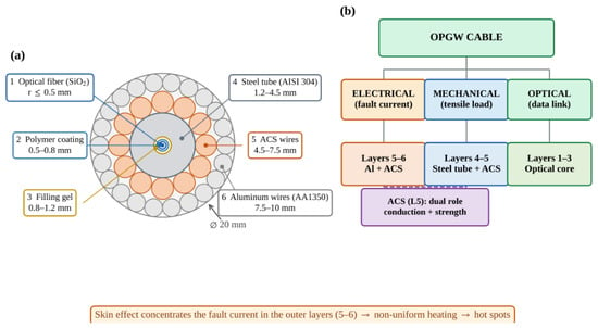
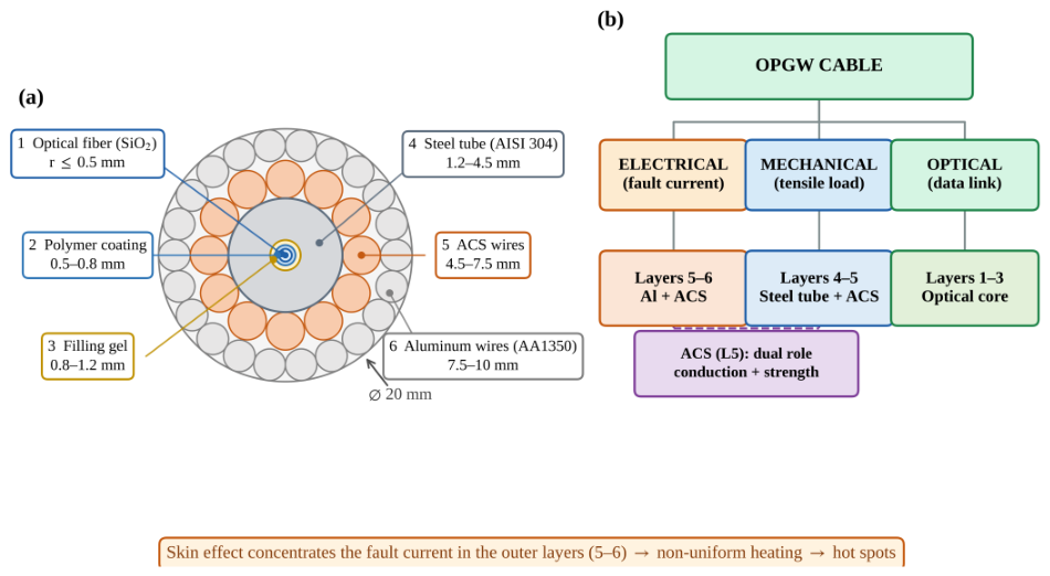
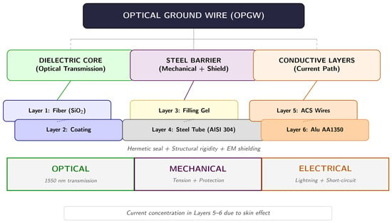
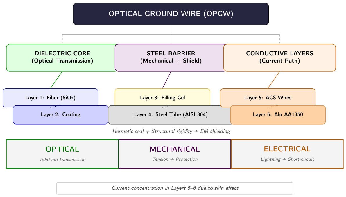
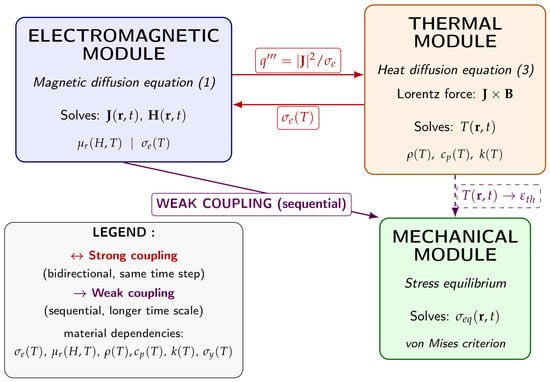
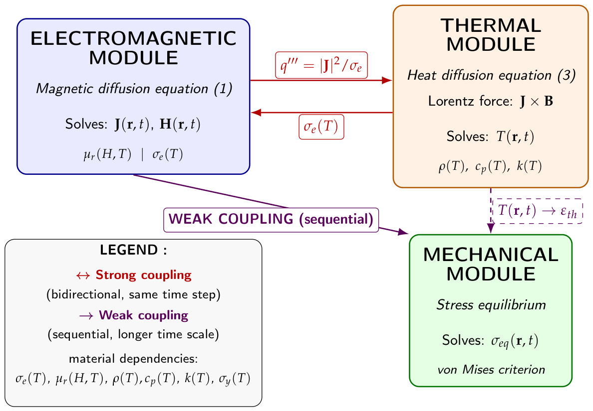
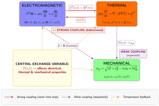
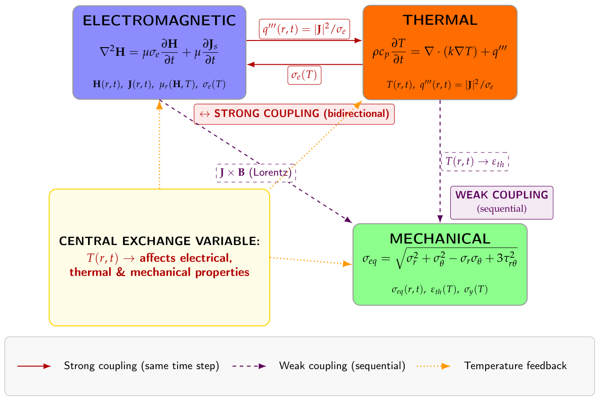
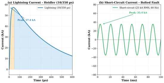
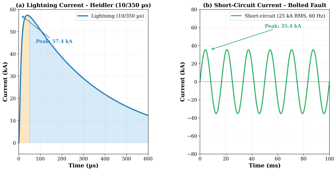
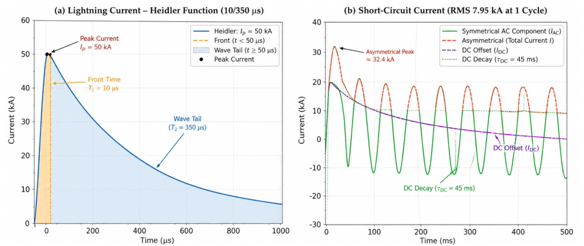
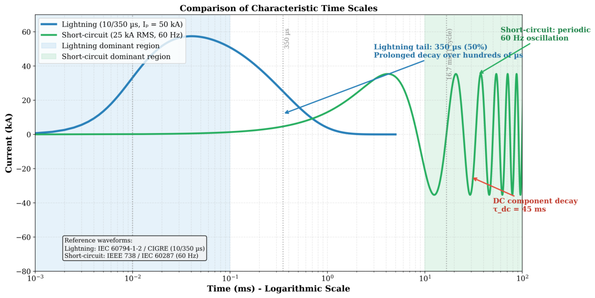
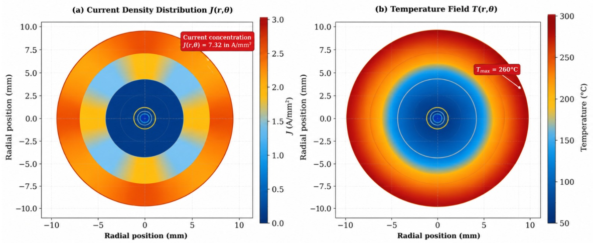
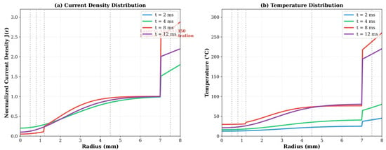
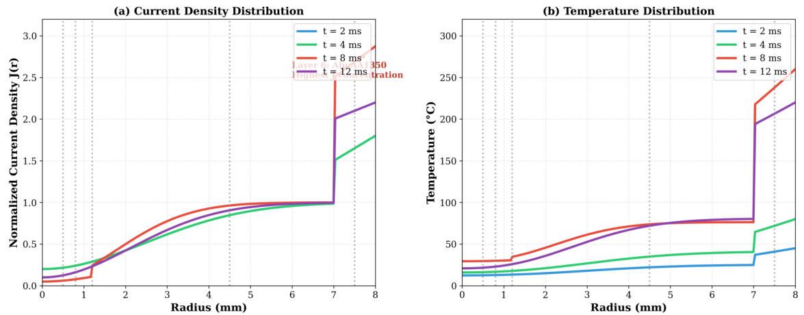
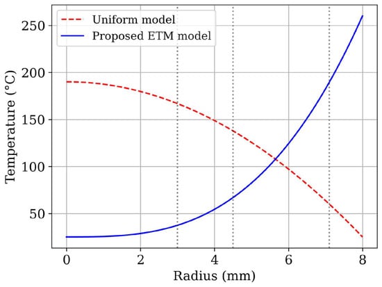
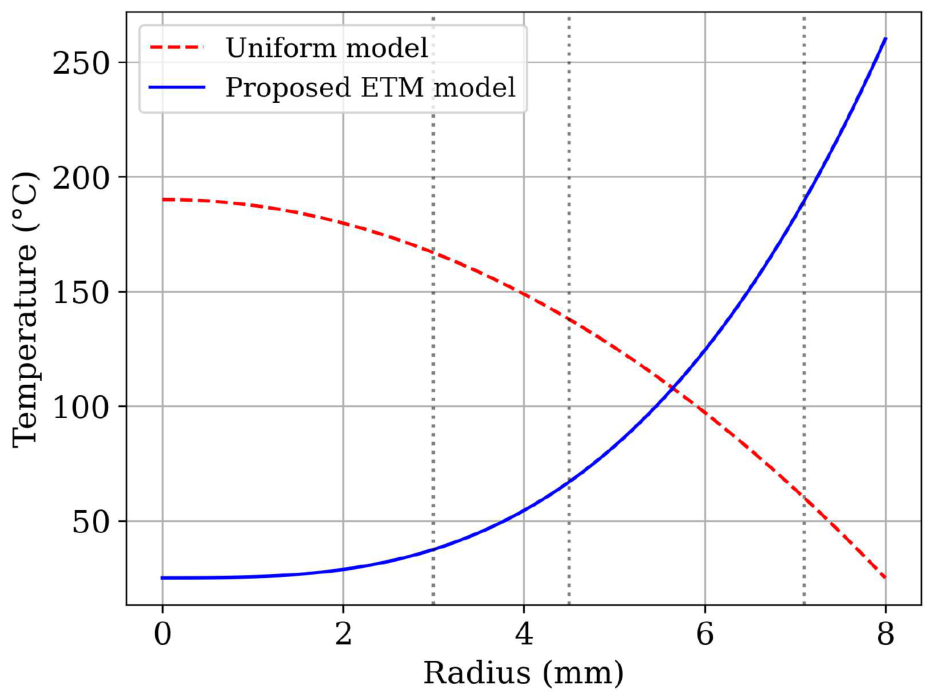
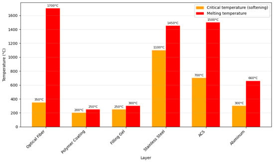
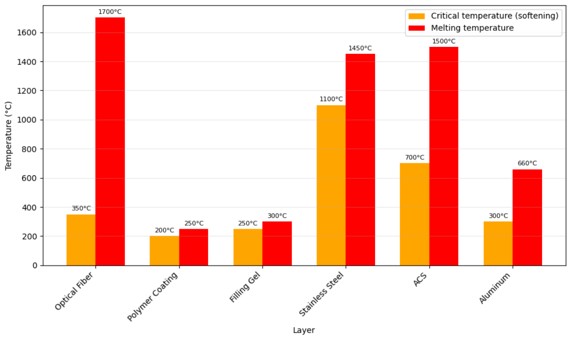
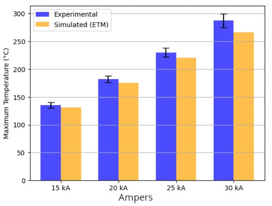
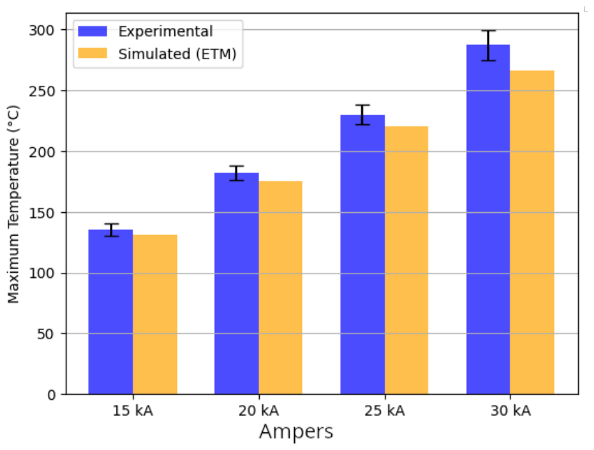
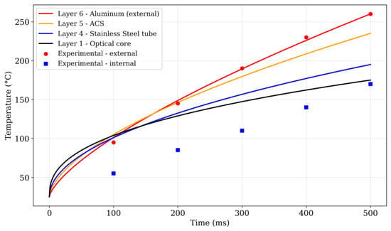
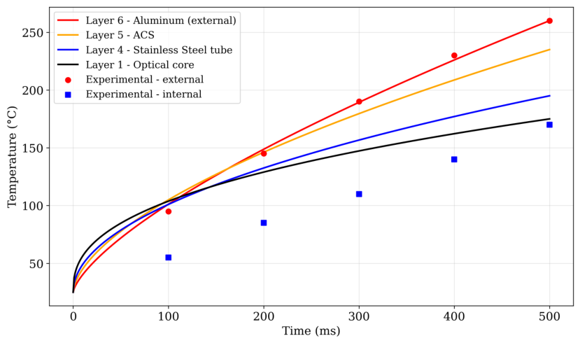
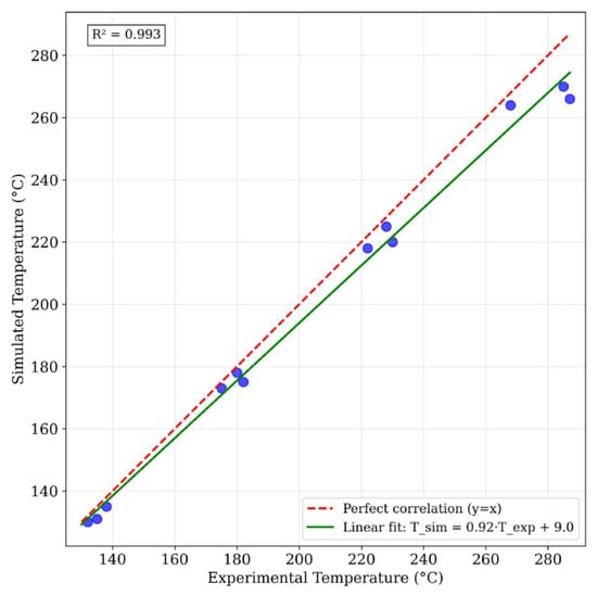
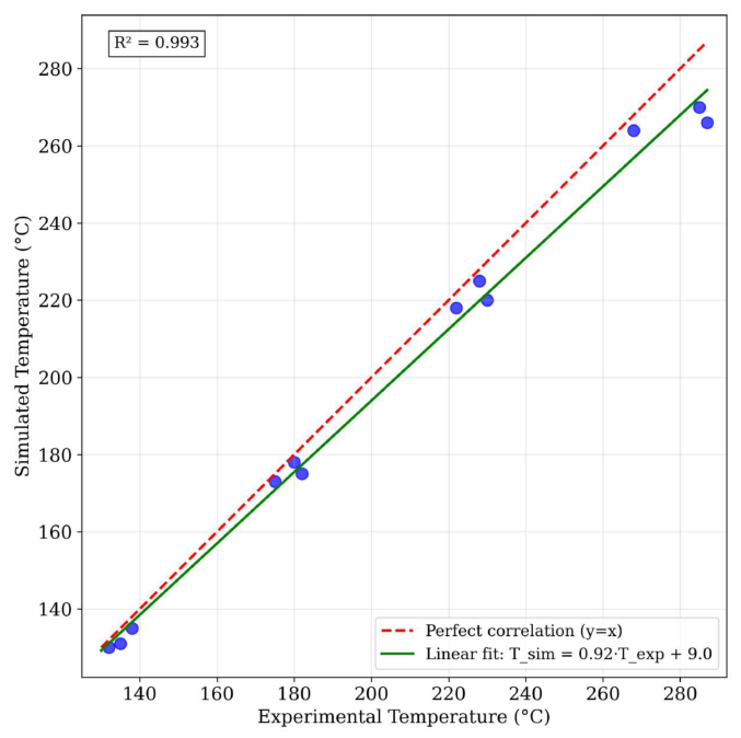
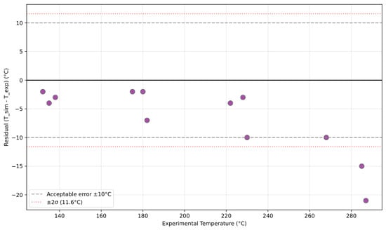
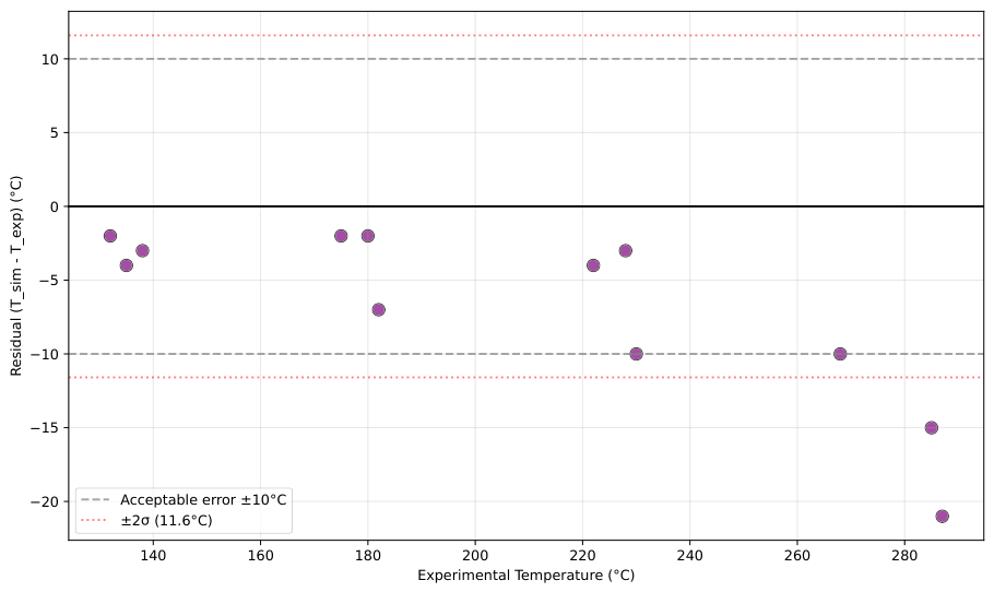
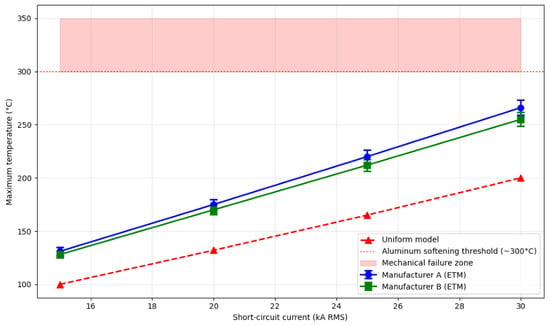
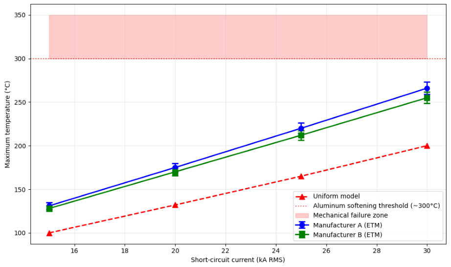
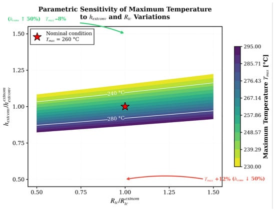
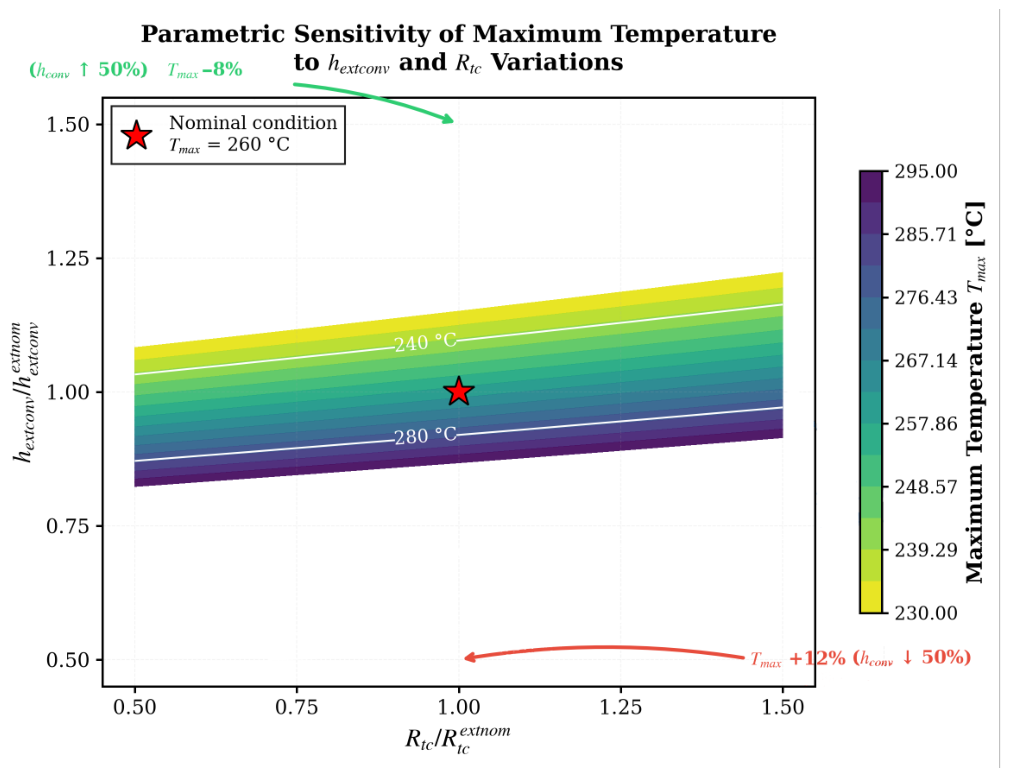
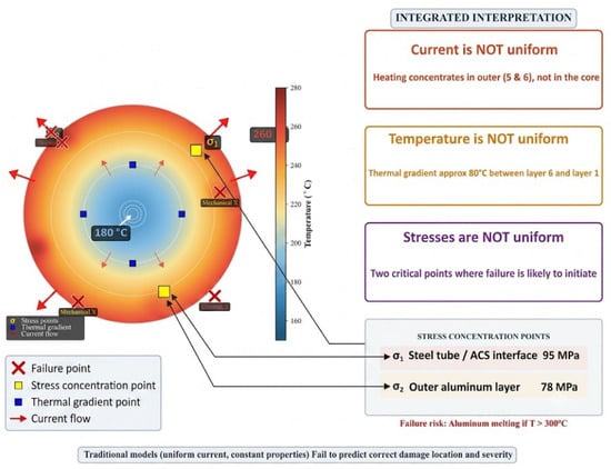
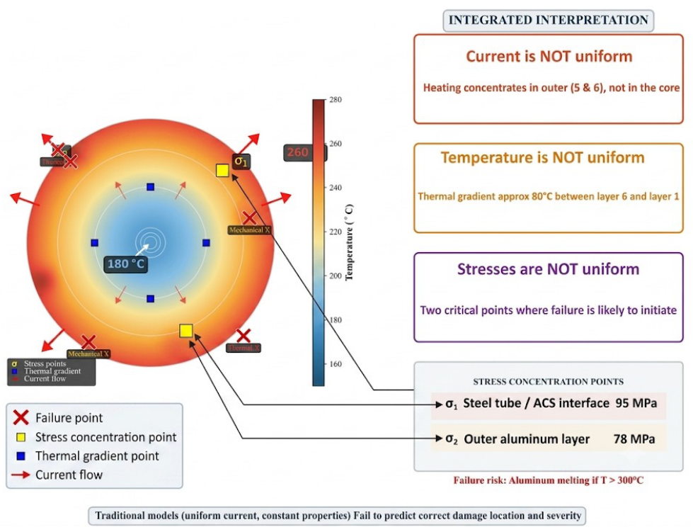
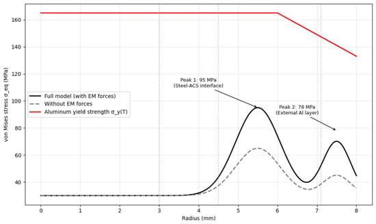
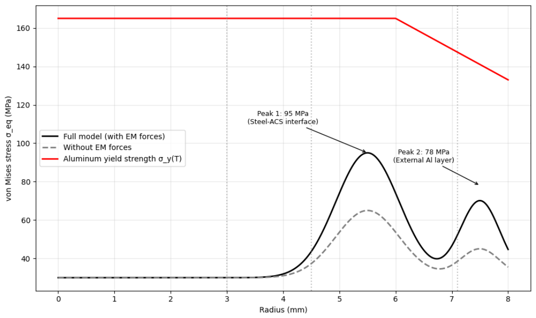
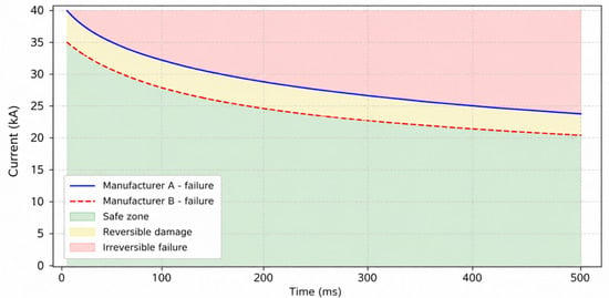
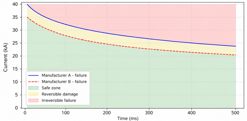
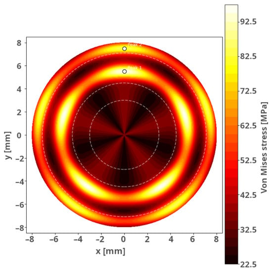
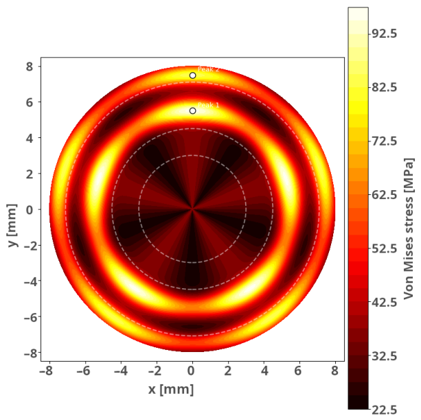
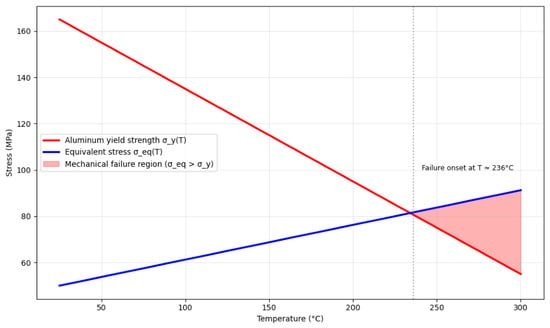
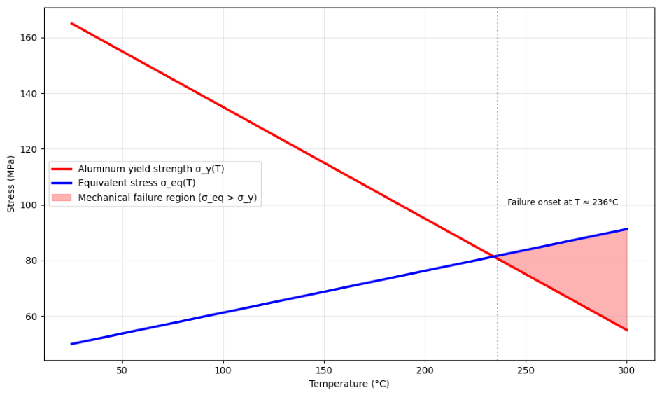
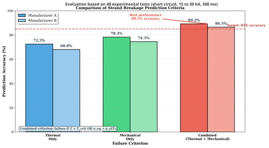
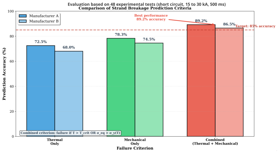

Disclaimer/Publisher’s Note: The statements, opinions and data contained in all publications are solely those of the individual author(s) and contributor(s) and not of MDPI and/or the editor(s). MDPI and/or the editor(s) disclaim responsibility for any injury to people or property resulting from any ideas, methods, instructions or products referred to in the content. |
© 2026 by the authors. Licensee MDPI, Basel, Switzerland. This article is an open access article distributed under the terms and conditions of the Creative Commons Attribution (CC BY) license.