


Abstract
To overcome the limitations imposed by the natural ionosphere on high-frequency (HF) communication systems, the generation of artificial electron clouds through space-based release of ionizable materials offers a controllable means of constructing localized plasma environments. However, a systematic mapping between release parameters and radio wave propagation characteristics is still lacking, which restricts engineering applications. This paper establishes a full-chain simulation framework that links release parameters, cloud morphology, and propagation characteristics by combining a two-fluid hydrodynamic model with ray tracing. Results show that as release altitude rises from 150 km to 210 km, the cloud undergoes pronounced stretching along the magnetic field (the cloud scale grows from 17.28 km to over 80 km), resulting in a broader signal shadow zone (expands from 116 km to 170 km) and a marked increase in multipath delay spread. Increasing mass from 4 kg to 12 kg raises peak electron density from 7.416 × 10¹² to 2.154 × 10¹³ m−3 and widens the shadow zone from 144 km to 174 km. Raising the ionization rate from 20% to 80% broadens the enhancement zone but reduces the shadow zone. Higher altitudes favor broad shielding, larger masses enhance scattering strength and duration, while higher ionization rates accelerate cloud evolution for rapid response and lower rates provide stable coverage. These findings can provide theoretical guidance for the precise design of artificial electron clouds tailored to different application requirements.
1. Introduction
The ionosphere, as a key component of the solar–terrestrial space environment, serves as the core channel supporting the operation of long-range information systems such as high-frequency communication and over-the-horizon radar (OTHR) [1,2]. However, due to factors such as solar activity and geomagnetic disturbances, the natural ionosphere exhibits significant spatiotemporal variability, leading to inherent bottlenecks for radio systems that rely on its reflection or scattering, including unstable communication quality and link interruptions [3,4,5]. Particularly under extreme conditions such as natural disasters and emergency rescue operations, conventional communication infrastructure may be damaged. In such scenarios, the availability of independently controllable, stable, and reliable emergency communication capabilities becomes especially critical.
Actively releasing specific chemical substances into the ionosphere to artificially modify the local plasma environment can generate artificial electron clouds with high-density gradients [6,7,8,9]. This approach offers a disruptive technological pathway for overcoming the limitations of the natural ionosphere and constructing predictable or even customizable “aerial information bridges”. Since the first sodium vapor tracer experiment conducted under “Project Firefly” in the 1950s, a series of notable active space release experiments, such as AMPTE, CRRES, and MOSC, have been carried out internationally [10,11,12,13]. Through the release of easily ionizable metals (e.g., barium (Ba), lithium (Li), strontium (Sr), samarium (Sm)) or electron-depleting substances (e.g., sulfur hexafluoride (SF6)), these experiments successfully produced artificial ionospheric disturbance regions of various morphologies—including enhancement clouds and holes—thereby demonstrating the feasibility of artificially manipulating the local ionospheric environment [14,15,16,17,18,19].
Substantial progress has been achieved in the theoretical and experimental research on artificial electron clouds over several decades. However, research on the applications of artificial electron clouds remains at an exploratory stage, with particularly limited studies on their radio wave propagation characteristics. Marmo et al. conducted early investigations into the propagation characteristics of artificial plasma clouds and developed a spherically symmetric Gaussian-distributed electron cloud reflection model in the very high frequency (VHF) band [20]. In recent years, ray-tracing methods have been widely applied in the analysis of radio wave propagation in the ionosphere, enabling effective simulation of propagation paths, multipath delays, and signal distributions of electromagnetic waves in inhomogeneous media [21,22]. Joshi et al. employed ray-tracing methods to study the influence of artificial plasma clouds on HF radio wave propagation [23]. Xie et al. investigated the effects of artificial plasma clouds on HF propagation paths and found that 10 MHz waves can generate up to four additional paths over a propagation distance of 500 km, while 15 MHz and 20 MHz waves can create new radio links [19,24]. Ma et al. analyzed the impact of ionospheric disturbances induced by rocket plumes on OTHR wave propagation and presented the variation patterns of absorption loss with frequency, elevation angle, solar activity, season, and time [25]. Zhao et al. further studied the radio propagation and scattering characteristics of artificial electron clouds using the geometrical theory of diffraction (GTD) [26].
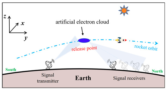
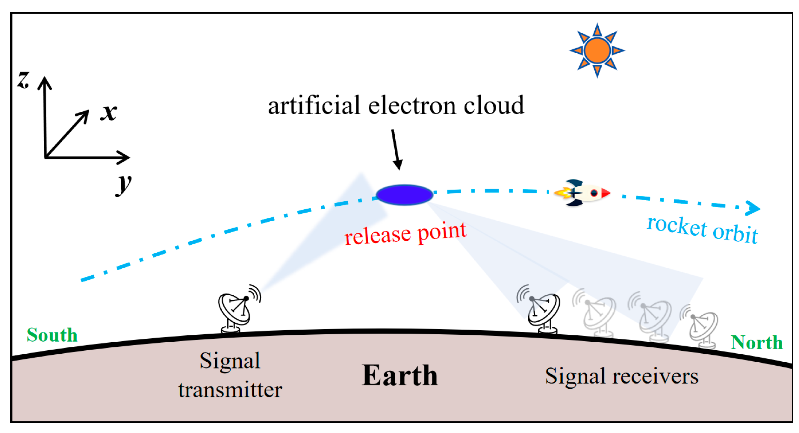
In summary, previous studies have primarily focused on the morphological evolution of artificial clouds and their background perturbation effects, but have not yet established a systematic quantitative relationship between release parameters and radio wave propagation characteristics. To address this gap, this paper employs a two-fluid dynamics model to calculate the spatial–temporal evolution of artificial electron clouds, combined with ray-tracing techniques to reconstruct realistic radio wave trajectories through the perturbed ionosphere, thereby constructing a comprehensive analytical framework linking “release parameters–cloud morphology–propagation characteristics.” Based on this framework, we systematically quantify the impacts of release altitude (150–210 km), mass (4–12 kg), and the initial ionization rate (20–80%) on key propagation metrics, including shadow-zone width, enhancement-zone width, and multipath delay spread. The findings provide important theoretical guidance for designing artificial electron clouds with controllable electromagnetic properties in practical communication or countermeasure scenarios. Figure 1 provides a schematic overview of the release geometry and simulation configuration described above.
Figure 1.
Schematic diagram of the simulation configuration.
2. Theoretical Model and Methods
2.1. Evolution Model of Artificial Electron Cloud
The release of neutral barium vapor in the ionosphere undergoes several stages. At early times (less than one collision time), the cloud expands as a self-collision fluid, pushing the ambient gas. As the expansion pressure of the released cloud diminishes, the released gas thoroughly mixes with ambient particles and gradually attains thermal equilibrium with the surrounding environment, thereby entering an extended free diffusion phase. Ion chemical reactions predominantly take place during this stage. The primary reactions of metallic barium in the ionosphere are as follows:
The reaction between Ba and atomic oxygen is neglected in this study, as its rate constant is substantially smaller than that of the Ba and molecular oxygen reaction [27].
The general diffusion equation for the neutral cloud particles is:
where represents the convection term, is the diffusion term. describes the loss due to ionization of the cloud, neglecting the variation in the incident solar flux in the ionosphere; is photoionization rate of barium, and equals 0.036 s–1. is the loss due to oxidation, in which is the number density of O2, and is the reaction constant [28]. The oxidation of Ba atoms may result from the reaction between Ba and molecular oxygen, or between Ba and atomic oxygen, but the latter reaction is insignificant at altitudes above 120 km. and are the density and the velocity of the neutral cloud, respectively. is the neutral diffusion coefficient [29], where is the total neutral particle number density of the background atmosphere; is the neutral temperature; is the reduced mass of the barium atom and the background neutral particle; and , , , and are the masses and atomic radii of the barium atom and the background neutral particle, respectively.
The density distribution of the barium cloud at the initial release stage is assumed to follow a Gaussian distribution:
where is the total number of barium atoms released, is the initial cloud radius, and is the position of a given point. The barium ion number density at infinity is assumed to be zero, and the boundary condition is given by . Solving with the initial and boundary conditions yields the following spatial distribution of the barium cloud as a function of time [30]:
where denotes the coordinates of the release point, and denotes the change in the center position of the cloud.
Ionization of the barium cloud gives rise to a localized plasma density enhancement in the ionosphere. Due to the different spatial distributions between barium ions produced by photoionization and the background ionospheric ions, the two ion species are treated separately. Furthermore, at the altitude under consideration, the background ion population consists predominantly of oxygen ions. Therefore, a two-component model comprising barium metal ions and oxygen ions is adopted herein. Neglecting variations in the background oxygen ion density induced by chemical reactions and assuming that the generation of the ion cloud results solely from photoionization, the general equations governing the plasma in the release region are as follows:
where the subscripts 1, 2, e, and s denote oxygen ions, metal ions, electrons and barium atoms, respectively. Equations (4) and (5) constitute the continuity equations for the ions. In the ionospheric F region, the quasi-neutrality holds (Equation (6)). The momentum equation for the ions is given by Equation (7), where , , , and denote the number density, mass, drift velocity, charge, and pressure of ion species j, respectively; is the convective derivative; and are the electric and magnetic fields; represents the momentum change; is the pressure gradient term; and denotes the total current density.
The momentum change terms for the oxygen ions and metal ions are given by:
where is the collision frequency between particle species (, denotes charged particles or neutral particles respectively). In addition to the momentum change arising from collisions, the momentum equation for ion species 2 should also include a momentum source term associated with the production of new ions. Due to the confining effect of the geomagnetic field, the velocity difference between charged particles in the direction perpendicular to the magnetic field is very small, and the corresponding collision terms can be neglected. Furthermore, neglecting electron inertia and treating the ion inertial term as a small perturbation, and assuming a constant geomagnetic field, the expressions for the drift velocities of the respective particle species can be obtained by solving the momentum equations [31]:
where ⊥ represents the component perpendicular to the magnetic field, and represents the component parallel to the magnetic field. denotes the unit vector along the magnetic field direction. is the gyro−frequency. The expressions for and are as follows:
The electric field is determined by , where is the background ambient electric field and is the perturbed electrostatic potential. Defining the effective potential as , the equation governing the effective potential derived from charge conservation is as follows:
where denotes the Pedersen conductivity, denotes the parallel conductivity, and represents the total electric charge.
By numerically solving Equations (3)–(15), the spatial distribution of the artificial plasma cloud in the release region can be obtained at any given time. The continuity Equations (4) and (5) are solved using the finite difference method. Equation (15) is an elliptic equation and is solved by means of the alternating direction implicit algorithm.
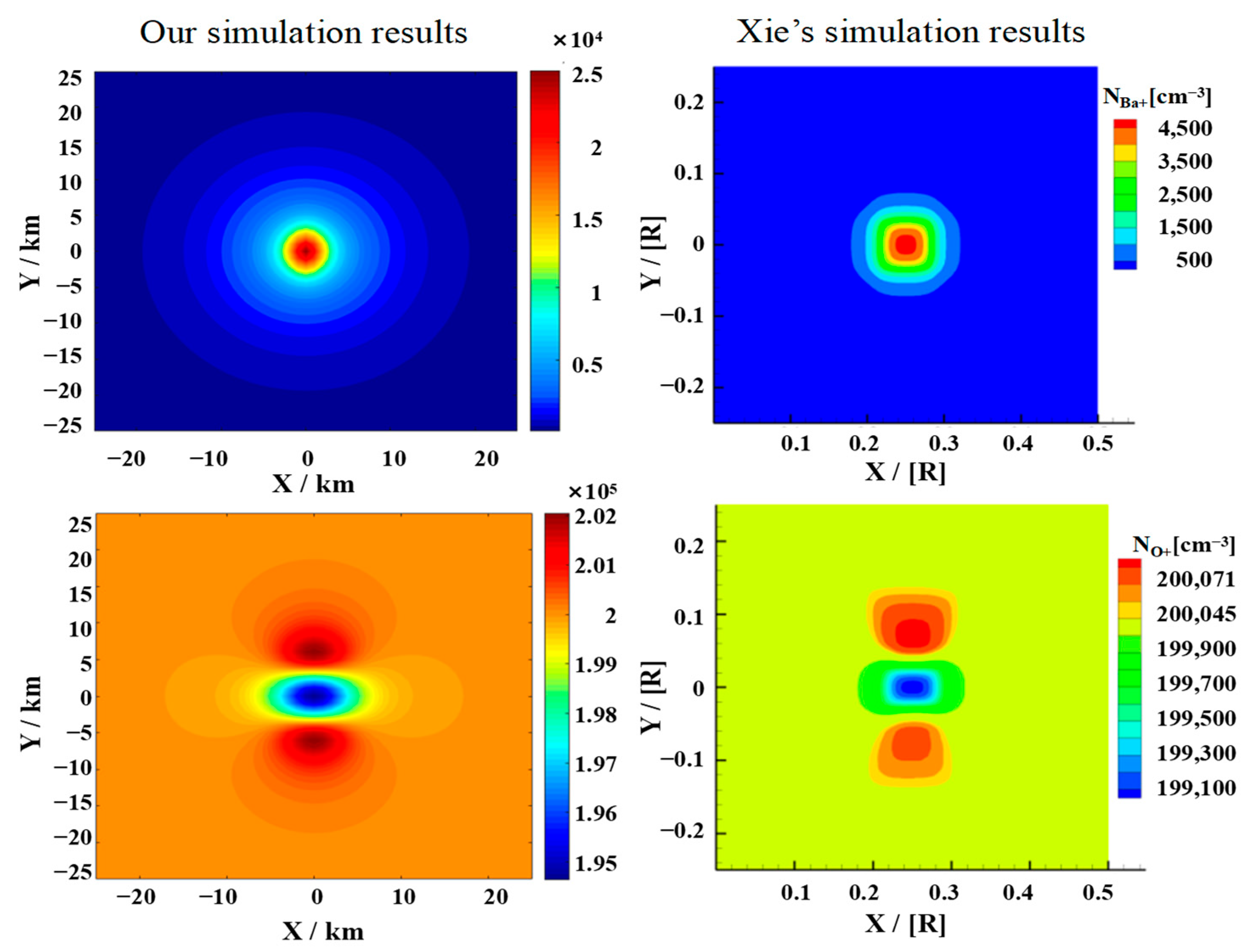
To validate the above-mentioned model, we compared the simulated plasma transport with the two-fluid results of Ma and Schunk [29] and the two-component MHD simulations of Xie [32]. Our calculated velocity fields of barium ions (Figure A1) and oxygen ions (Figure A2) at 2 s reproduce the anisotropic barium-ion expansion along the magnetic field and the accompanying “snowplow” perturbation of background oxygen ions, with magnitudes and spatial patterns consistent with Ma and Schunk’s results. Additionally, our density distributions of barium ions and oxygen ions at 1 s (Figure A3) and 5 s (Figure A4) match the characteristic structures reported by Xie [32], including the central oxygen-ion depletion and flanking enhancements. These validation tests confirm that our framework reliably captures the essential physics of artificial cloud formation and early-time plasma dynamics, justifying its use in the parametric study below.
2.2. Ray Tracing Technique
Artificial electron clouds are localized high-density plasma regions formed by releasing alkali earth metals or other substances into the ionosphere. They can serve as scattering media for applications such as over-the-horizon communication and electronic countermeasures. Their electromagnetic effectiveness depends not only on the electron density distribution of the cloud but also on its geometric morphology, spatial orientation, and evolutionary process. In recent years, the ray-tracing technique has been widely adopted in the analysis of radio wave propagation in the ionosphere, enabling effective simulation of propagation paths, echo signal distributions, and multipath delays of electromagnetic waves in inhomogeneous media [33,34,35].
Based on the electron density distribution of the cloud, this paper employs the ray-tracing technique to calculate the propagation paths of electromagnetic waves in the ionosphere and the artificial electron cloud. Letting the group path , the three-dimensional ray-tracing equations for the group path in spherical coordinates can be written in component form as follows:
Here, , , are the spherical coordinates of a point on the ray path, and , , are the three components of the wave vector in the spherical coordinate system, satisfying , where ω is the angular frequency of the wave; c is the speed of light; and the Hamiltonian H is:
where is the refraction index of the medium, in which , is the plasma frequency, and f is the frequency of the wave; the imaginary part is neglected because collision losses are small at HF for the altitudes considered. For given initial values, the ray equations are solved iteratively using the Runge–Kutta method to obtain the coordinates and wave vector at each point along the ray path [36,37]. Connecting all these points yields the complete ray trajectory.
2.3. Parameter Settings
The background atmospheric density, ionospheric particle number densities, temperature, and magnetic field, are obtained from the NRLMSIS 2.1 atmospheric model, the IRI-2020 ionospheric model, and the DGRF/IGRF 1945–2030 magnetic field model, respectively. All boundary conditions are implemented using a constant-value extrapolation scheme. In the simulation of artificial electron clouds, the Cartesian coordinate system is established with the x-axis pointing in the east–west direction, the y-axis pointing in the north–south direction (along the direction of the magnetic field), and the z-axis pointing in the altitude direction. The time step is set to 0.01 s, and the spatial grid spacing is set to 1 km. Detailed parameters are provided in Table 1.
Table 1.
The main simulation parameters of artificial electron cloud.
In ray-tracing, the spherical coordinate system is adopted, with the release center serving as the coordinate origin, the spatial step size is set to 1 km, and the integration step size is 0.05 km. The relevant parameters are summarized in Table 2. The ray tracing setup is configured as follows. The transmitter is fixed at a ground distance of 200 km south of the cloud’s ground projection. On the ground, receivers are placed from 100 km to 400 km south of the projection, with a uniform spacing of 2 km. A total of 683 rays are launched, with elevation angles uniformly sampled from π/6 to π/3 at a step of π/4096 rad. The inclination, path, and final landing position of each ray can be uniquely determined by ray tracing. If the final landing position of a ray on the ground is within 1 km of a certain receiver position, it is considered an effective echo signal received, and different echo signals are distinguished by the emission inclination and group path. The background level used for defining shadow and enhancement zones is obtained by performing ray tracing under exactly the same configuration but without the artificial electron cloud. The background amplitude at each receiver is simply the number of rays that reach that receiver in the undisturbed ionosphere. In the presence of the cloud, the relative amplitude at a receiver is defined as the ratio of the received ray count (with cloud) to the background count at that receiver, expressed as a percentage. We define the shadow zone as the contiguous ground region where this relative amplitude falls below 30% of the background, and the signal enhancement zone as the region where it exceeds 120% (i.e., more than 20% above background). This normalization makes the thresholds independent of the absolute ray density and allows consistent comparison across different release conditions.
Table 2.
The main simulation parameters of ray tracing.
3. Results and Discussion
The density distribution, geometric morphology, and evolution process of artificial electron clouds vary under different release conditions (e.g., release altitude, initial cloud density), leading to different scattering effects on electromagnetic signals. Therefore, this section analyzes the propagation characteristics of artificial electron clouds under various release conditions through multiple simulation cases. The effects of several release parameters, including release altitude and mass, on radio wave propagation characteristics are systematically investigated, and the mechanism by which release parameters regulate the electromagnetic performance of artificial electron clouds is presented.
3.1. Propagation Characteristics at Different Release Altitudes
Here we present the simulation results of artificial electron clouds generated by barium release at different altitudes (150 km, 180 km, and 210 km), and analyze the effects of release altitude on cloud morphology and radio wave propagation characteristics. All simulation cases employ the same release mass (10 kg) and ionization rate (20%), and the release is conducted in a static, point-source manner.
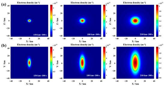
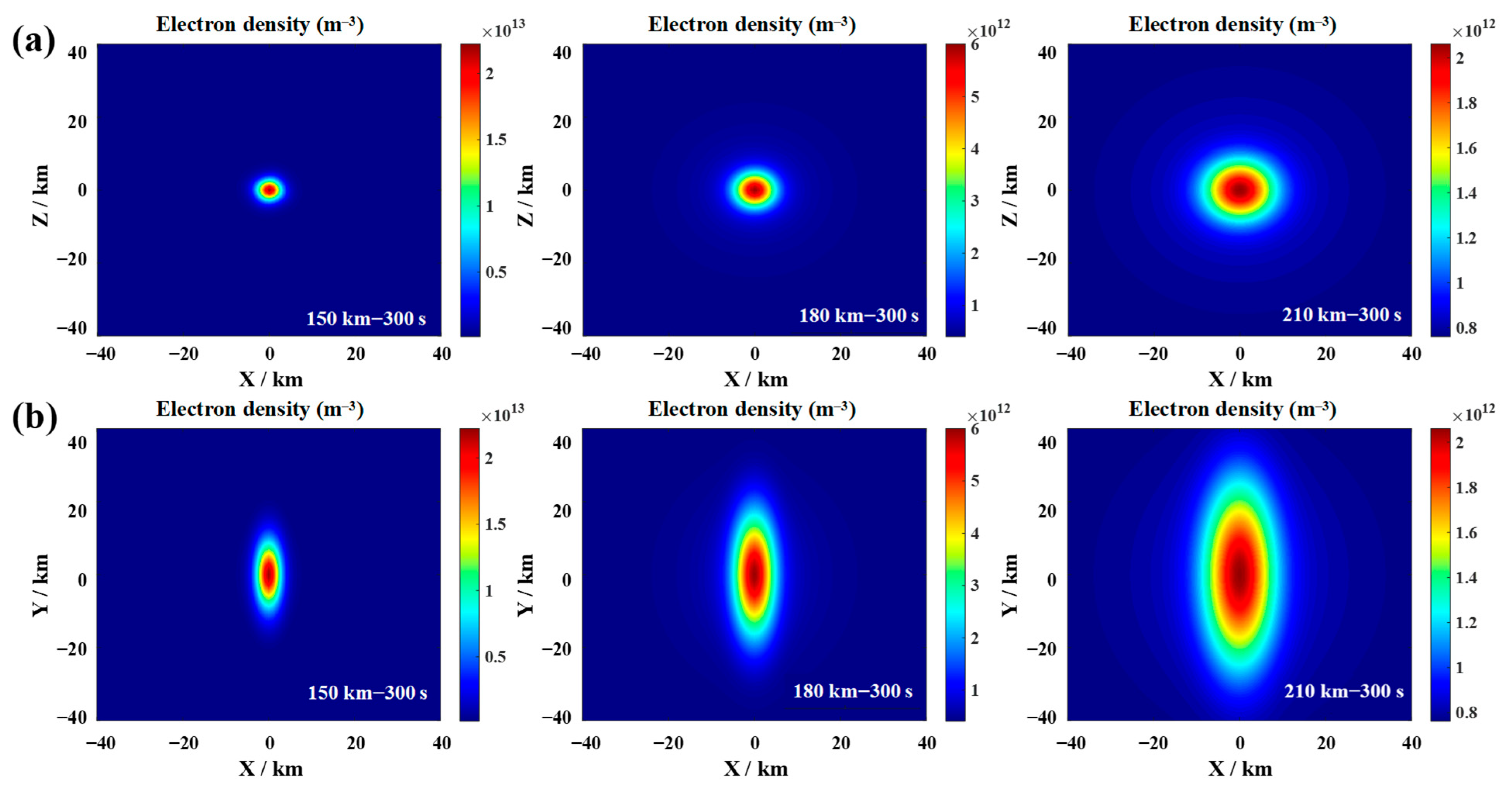
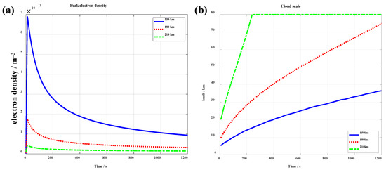
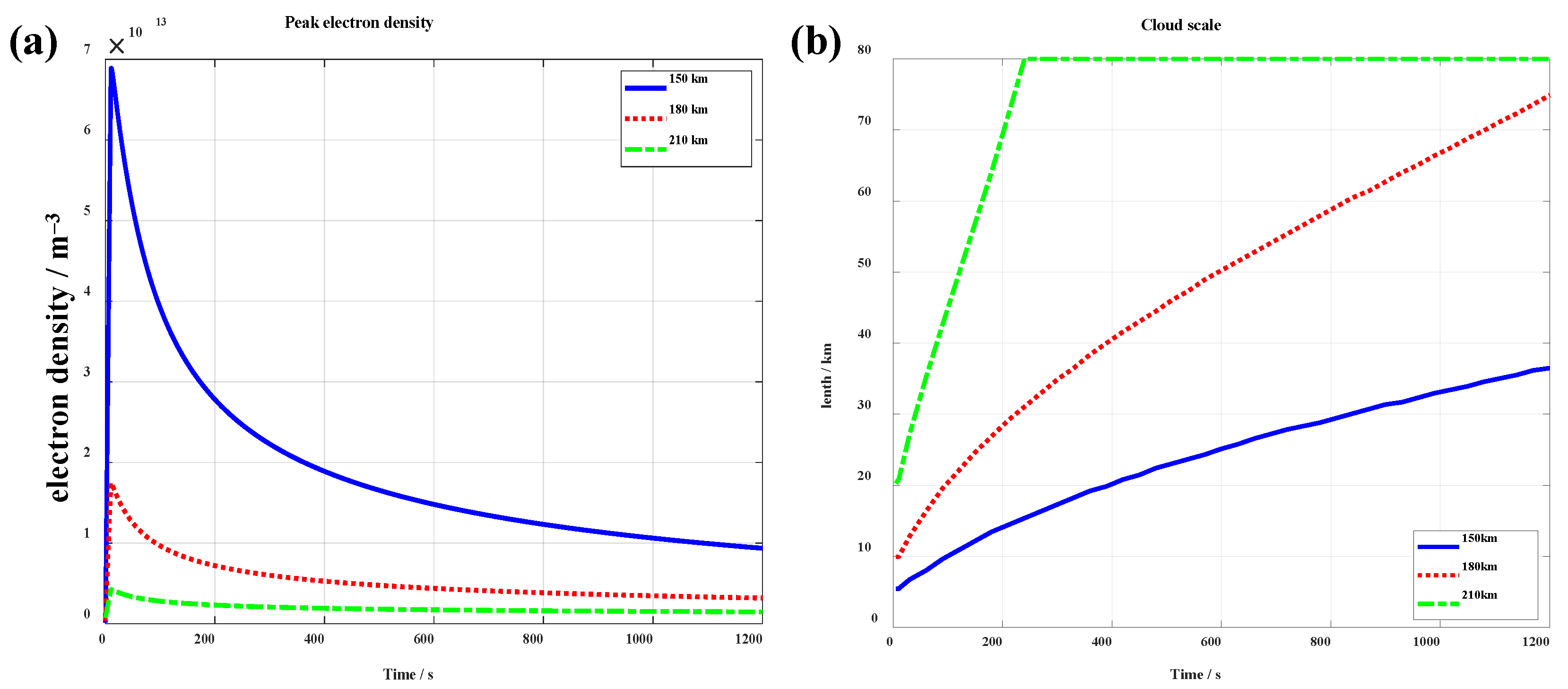
Figure 2 presents the electron density distributions for plasma clouds released at different altitudes. At lower release altitudes, the ambient neutral atmosphere is denser, resulting in high collision frequencies between ions–neutrals and electrons–neutrals. Under these conditions, the collisional drag plays a dominant role, strongly suppressing plasma diffusion. Consequently, the generated electron cloud remains compact and spatially localized. In contrast, at higher release altitudes, the collision frequency drops sharply, allowing the geomagnetic field to exert progressively stronger guiding and confining effects. As a result, the ion cloud expands rapidly along the magnetic field, adopting an elongated ellipsoidal morphology with significantly increased spatial extent. Consistent with this trend, peak electron density is highest at the lowest release altitude (150 km) for a fixed barium mass release, owing to tighter initial confinement and reduced radial diffusion. However, enhanced oxidation loss—driven by elevated O2 concentration at lower altitudes—accelerates electron recombination, leading to faster decay of electron density compared to higher-altitude releases (Figure 3). To quantitatively characterize cloud morphology, we define the cloud boundary as the isosurface on which the electron density falls to 1/e of the central maximum. Under the combined effects of collisions, the geomagnetic field, and other external forces, the cloud size increases with release altitude. At 300 s, the cloud sizes at 150 km, 180 km, and 210 km are 17.28 km, 34.88 km, and >80 km, respectively (note that at 210 km, the cloud size had already exceeded the computational threshold by approximately 240 s after release).
Figure 2.
Morphological distribution of artificial electron clouds at different release altitudes (150, 180, 210 km) at 300 s after release, with a release mass of 10 kg and ionization rate of 20%. (a) X–Z plane; (b) X–Y plane.
Figure 3.
Temporal evolution of (a) peak electron density and (b) cloud scale for release altitudes 150, 180, and 210 km, with a release mass of 10 kg and ionization rate of 20%.
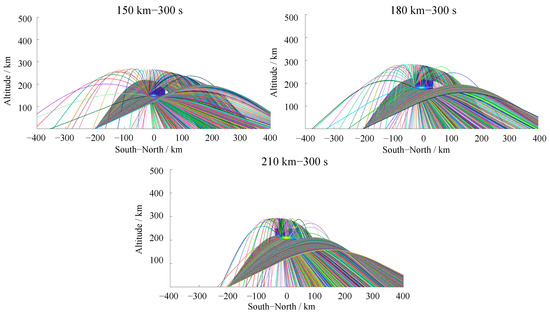
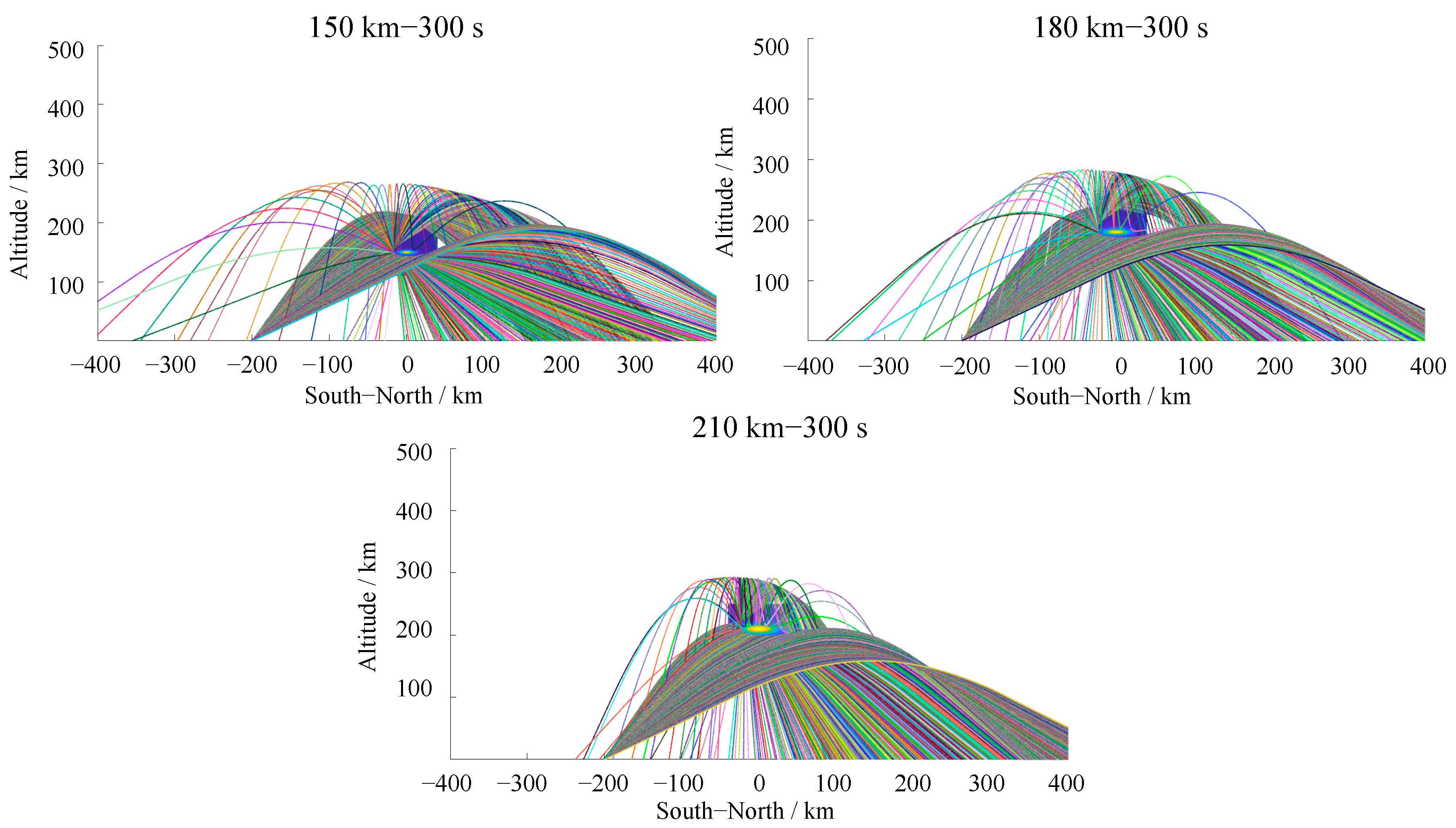
To further analyze the influence of release altitude control on the communication performance of artificial electron clouds, we conducted ray-tracing simulations. The transmitter was assumed to be located 200 km south of the ground projection of the electron cloud center, thereby establishing an oblique propagation. Simulations employed a fixed carrier frequency of 10.8 MHz and systematically varied the ray elevation angle from π/6 to π/3. Figure 4 presents the ray trajectories for clouds released at 150 km, 180 km, and 210 km after 300 s. As shown in Figure 4, rays traversing the cloud volume undergo pronounced refraction and scattering due to sharp electron density gradients, leading to pronounced changes in the ray propagation paths. Ground-received signals originate from three dominant mechanisms: (i) directly reflected by the ionosphere, (ii) quasi-specular reflection directly from the dense core of the cloud, and (iii) cloud-induced ray bending followed by subsequent ionospheric reflection—a hybrid “cloud–ionosphere relay” path. At lower release altitudes, collisional damping suppresses field-aligned structuring, yielding a compact, high-density cloud that acts as an efficient wide-angle scatterer; consequently, the echo footprint on the ground is broader.
Figure 4.
Ray-tracing results for artificial electron clouds at different altitudes (150, 180, 210 km) at 300 s after release, operating frequency 10.8 MHz, transmitter located 200 km south of the cloud’s ground projection.
In addition, the presence of the artificial electron cloud produces a certain “shielding” effect on the radio signals, creating a localized signal “shadow zone” (i.e., the contiguous ground region where the received signal amplitude falls below 30% of the background level) behind the cloud. Affected by the release altitude and cloud geometry, the location of the signal shadow zone on the ground varies with altitude. With increasing release altitude, the signal shadow zone shifts progressively closer to the transmitter and widens horizontally. Specifically, at the release at 150 km, the overall scale of the cloud is small, and its ability to deflect rays is limited. The horizontal extent of the signal shadow zone is only 116 km, and a small amount of scattered signal energy leaks into this region. When the release altitude increases to 180 km, the electron cloud forms a longer distribution axis along the magnetic field, the range of affected rays expands significantly, the horizontal extent of the signal shadow region increases to 164 km, and the deflected rays also form two distinct signal focusing zones on either side. At 210 km, the major axis length of the electron cloud increases further, the overall coverage of the cloud becomes broader, and the horizontal extent of the signal shadow zone expands to 170 km. With the release altitude increasing from 150 km to 180 km and 210 km, the center of the signal shadow zone shifts progressively to the left, and its corresponding positions are 412 km, 334 km, and 253 km, respectively.
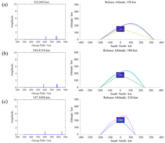
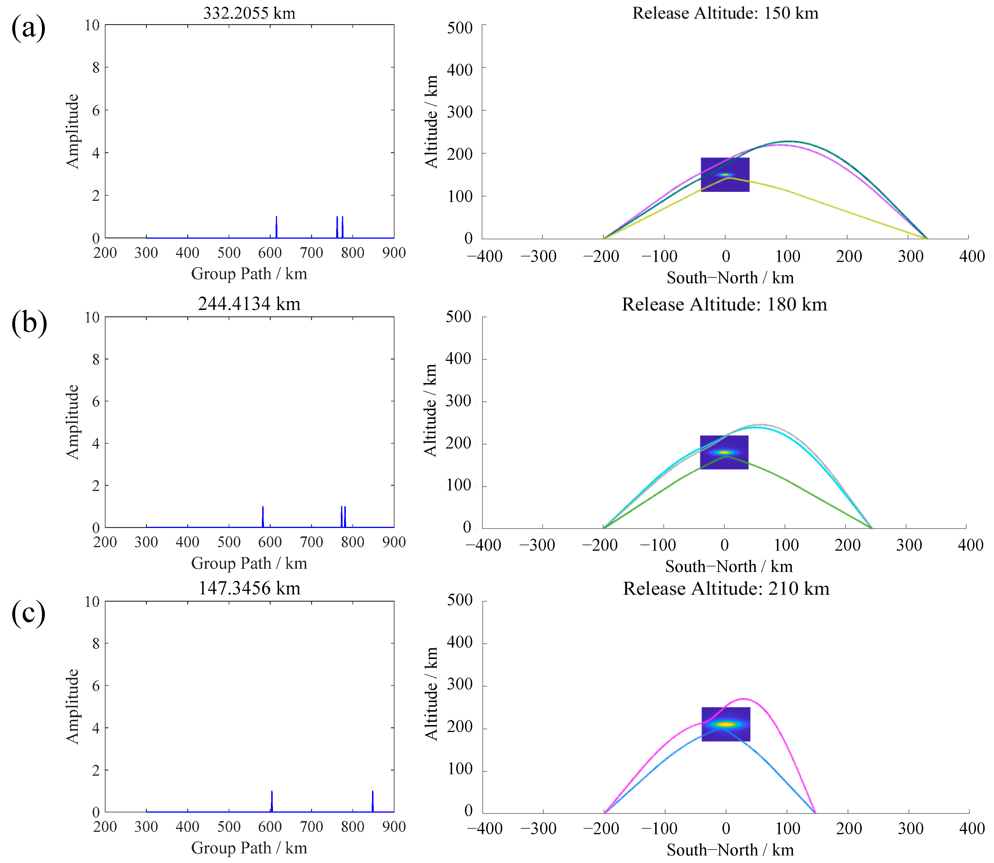
The presence of artificial electron clouds induces pronounced multipath propagation in signals traversing the cloud region. Based on ray tracing, we synthesize group path–amplitude diagrams and associated ray trajectories for ground-based receivers at various locations. Figure 5 shows typical multipath effects produced by clouds at different altitudes at 300 s, with the left panels presenting the group path–amplitude plots and the right panels the ray propagation paths. In the group path–amplitude diagram, each peak corresponds to an echo received at a specific receiver. The horizontal coordinate of the peak denotes the group path (i.e., the effective propagation distance), while its vertical coordinate represents the amplitude—quantifying either the measured echo intensity in the experimental detection or, in ray tracing-based synthesis, the number of rays arriving at that receiver. Notably, although echo amplitudes vary significantly in practical measurements due to attenuation, scattering, and instrumentation effects, the amplitude axis in the synthesized diagram reflects ray multiplicity rather than physical signal strength. The observed echoes comprise two primary contributions: (i) signals directly reflected from the artificial electron cloud, and (ii) signals first refracted or scattered by the cloud and subsequently reflected by the ambient ionosphere. This causes the echo signals arriving at the same receiver to have different group paths, i.e., the multipath effect.
Figure 5.
Partial echoes and corresponding ray paths at 300 s after release for release altitudes of (a) 150 km, (b) 180 km, and (c) 210 km. All cases assume a frequency of 10.8 MHz, the transmitter located at 200 km south of the cloud projection, and receiver stations at ground distances of 322.2055 km, 244.4134 km, and 147.3456 km, respectively.
The multipath delay spread—defined as the maximum group-path difference among detectable echoes at a given receiver—exhibits a strong positive correlation with release altitude; higher altitudes lead to significantly larger group-path spreads. It can also be roughly seen from Figure 5 that the magnitude of multipath delay exhibits a robust positive correlation with release altitude: higher release altitudes produce markedly larger group-path spreads at identical receiver locations. This is mainly because electron clouds at higher altitudes have larger dimensions; as the rays pass through the cloud, more scattered components with different paths are generated, and the path differences among these components increase with the cloud size, thereby enlarging the signal delay. This trend arises primarily because electron clouds released at greater altitudes exhibit larger spatial extents and higher integrated electron content, leading to stronger and more heterogeneous ray bending. Consequently, rays traversing such clouds sample a broader range of deflection angles and path lengths, increasing inter-ray path differences—and thus widening the temporal separation (group-delay spread) among multipath components.
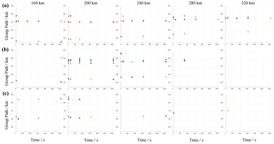
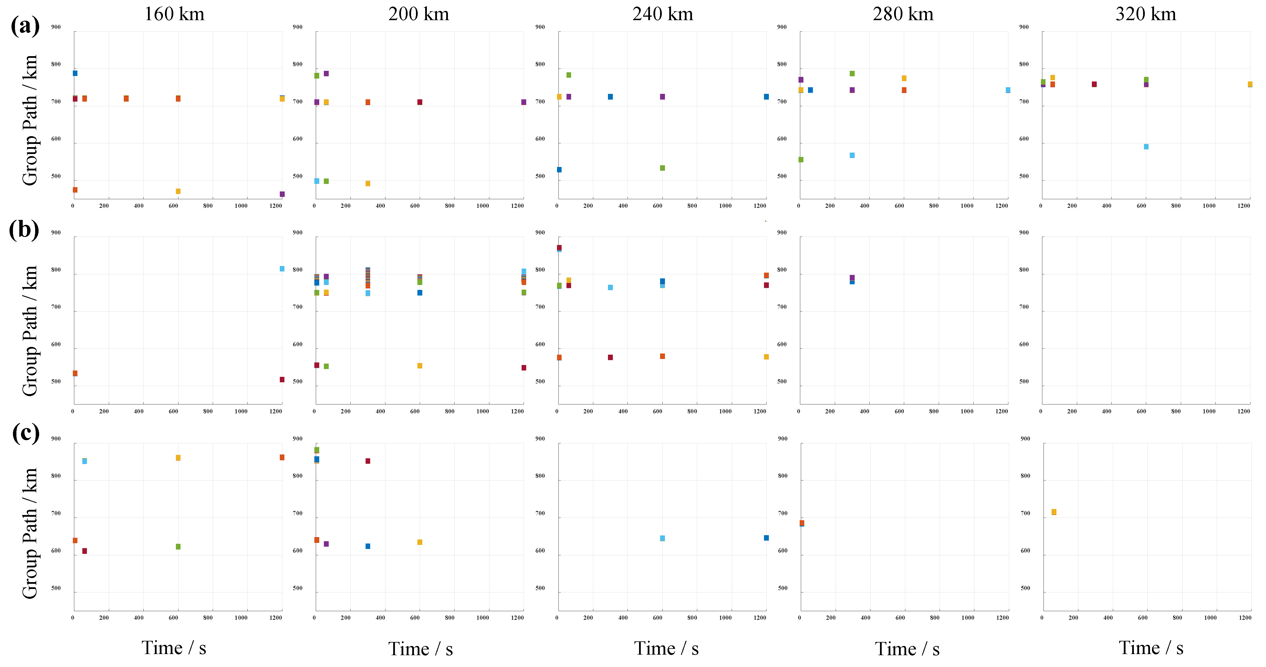
Figure 6 presents the group path–time evolution diagrams of echo signals received by ground-based receivers at varying positions for three release altitudes (150 km, 180 km, and 210 km). The results demonstrate that release altitude exerts a pronounced control over both the spatial distribution of echo intensity and the morphology of multipath structure. At 150 km, echoes with group paths in the 720–780 km range exhibit temporal stability, indicating their origin in reflection from the undisturbed natural ionosphere, unaffected by the artificial electron cloud. In contrast, echoes near the 500 km group path arise predominantly from direct reflection off the artificial electron cloud. Under this altitude, all receiver locations yield continuous, detectable echoes throughout the observation period, confirming only weak radio-wave shielding by the cloud. At 180 km, a strong spatial dependence emerges: receivers located between 200 km and 240 km record consistently strong and temporally coherent echoes—characteristic of a stable, cloud-dominated reflection path. Receivers at far distances (>240 km) are markedly affected by the cloud shielding effect, with echoes suffering substantial attenuation; the few echo signals received by nearby receivers (<200 km) are mainly formed by cloud reflections. At the release altitude of 210 km, the cloud size further increases. The signal strengths received by receivers in the range of 160–320 km are generally weak, the cloud shielding effect is pronounced, and the multipath effect becomes less evident at this stage.
Figure 6.
Group path–time diagrams for receivers at various ground positions for release altitudes (a) 150 km, (b) 180 km, and (c) 210 km. All simulations assume a release mass of 10 kg, an ionization rate of 20%, a probing frequency of 10.8 MHz, and a transmitter position at −200 km.
3.2. Propagation Characteristics with Different Release Masses
The release mass directly governs the electron density and lifetime of the artificial electron cloud, thereby influencing the critical frequency and the effective communication duration—defined as the time interval from release during which the cloud-induced echo amplitude remains above 50% of the background level. This section presents the evolution characteristics of the artificial electron cloud under different release masses of 4 kg, 8 kg, and 12 kg, and analyzes the effects of release mass on cloud morphology, electron density distribution, and radio wave propagation characteristics.
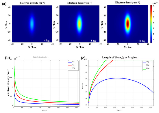
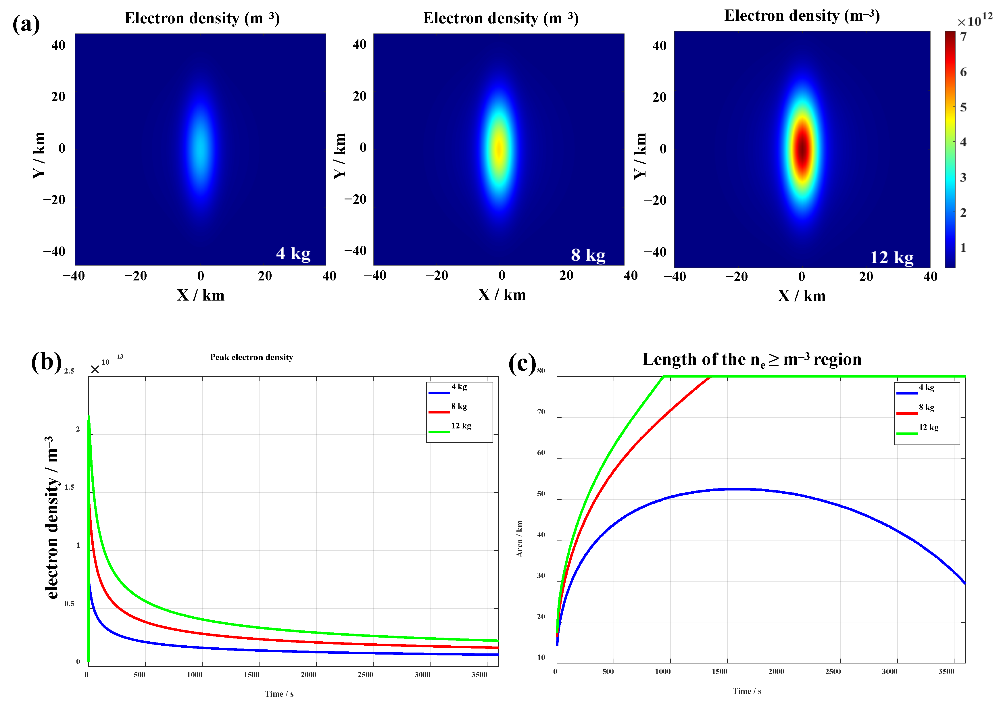
Figure 7 shows the spatial distribution and temporal evolution of the number density of the artificial electron cloud under different release masses. As can be seen from Figure 7a, qualitatively, the ionospheric disturbances induced by the various release masses share a common structure. A larger release mass yields a higher peak electron number density, and the peak density exhibits an approximately linear proportional relationship with the release mass; the maximum electron number densities for release masses of 4 kg, 8 kg, and 12 kg are 7.42 × 10¹² m−3, 1.45 × 10¹³ m−3, and 2.15 × 10¹³ m−3, respectively. As the release mass increases, the initial pressure gradient of the neutral cloud strengthens, which accelerates the field-aligned expansion rate of the particles along the geomagnetic field direction and correspondingly increases the decay rate of the electron number density. Meanwhile, a larger release mass also expands the spatial scale of the disturbance (Figure 7b) and prolongs the period during which the electron density remains significantly above the background level. To facilitate the comparison of the cloud size under different release masses, we adopt a threshold of 1012 m−3 and measure the length of the region where the electron density exceeds this threshold (as shown in Figure 7c). The results show that, dominated by field-aligned diffusion, this length increases continuously with time. Specifically, for the 8 kg and 12 kg cases, the threshold region length reaches 80 km at approximately 1350 s and 940 s, respectively. In contrast, for the 4 kg case, owing to the lower initial density and the weaker driving force for diffusion, the threshold region length reaches its maximum value (about 65 km) only at around 1500 s, after which it gradually contracts under the combined effects of diffusion and oxidation reactions.
Figure 7.
Morphological distribution and evolution of artificial electron clouds for different release masses (4, 8, 12 kg) at an altitude of 180 km and ionization rate of 20%. (a) Electron density distributions at 300 s; (b) peak electron density evolution; (c) length of the region with electron density > 1012 m−3.
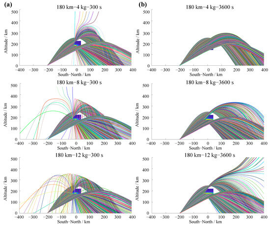
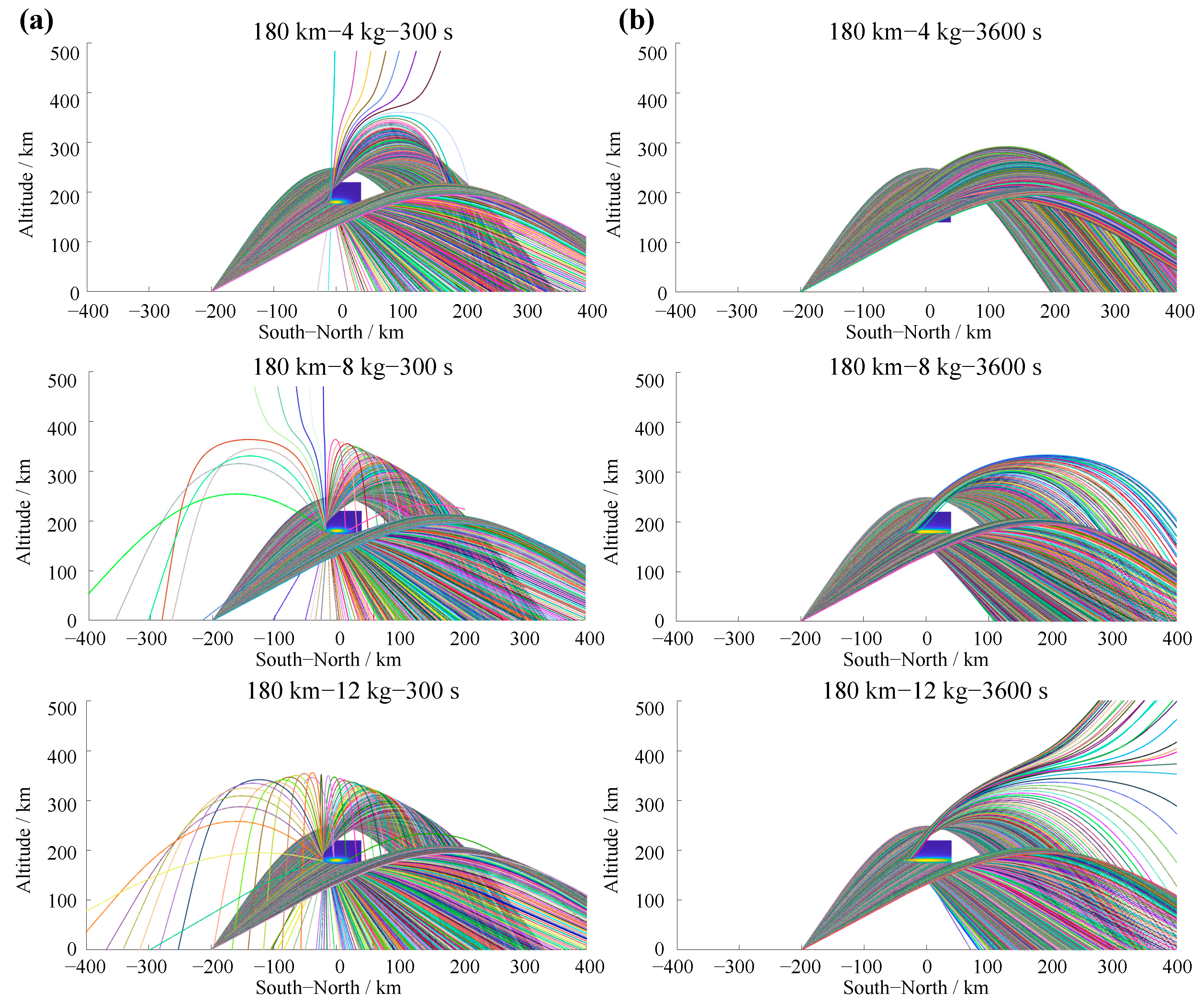
The ray-tracing results for the artificial plasma clouds generated at 300 s and 3600 s after the release of different masses of barium are shown in Figure 8, with an operating frequency of 12.8 MHz. A higher operating frequency is selected in this case because a larger release mass leads to a higher peak electron density, which in turn raises the plasma critical frequency; consequently, using a higher frequency enhances sensitivity to variations in release mass and thus more clearly reveals its influence on radio wave propagation diagnostics. As can be seen from Figure 8, the propagation paths of the rays are significantly altered after they pass through the artificial electron clouds produced by different release masses. As the release mass increases, both the electron density and the spatial extent of the cloud grow, resulting in increased ray deflection and a stronger scattering cross section. The signal shadow zone behind the cloud accordingly broadens, measuring 144 km, 158 km, and 174 km for the 4 kg, 8 kg, and 12 kg cases, respectively. A comparison of the results at 300 s and 3600 s reveals that, as time evolves, the cloud gradually diffuses over a wider region while its density continuously decreases, and its scattering effect on the signals weakens progressively. By 3600 s, the cloud generated by the release of 4 kg of barium has essentially lost any discernible scattering effect, and the scattering effects of the clouds produced by 8 kg and 12 kg of barium are also significantly diminished. These results demonstrate that, for a given operating frequency, the release mass not only governs the initial scattering capability of the artificial cloud but also dominates the temporal persistence of its radio wave control effect.
Figure 8.
Ray-tracing results for different release masses (4, 8, 12 kg) at an altitude of 180 km, ionization rate of 20%, operating frequency of 12.8 MHz, and the transmitter located 200 km south of the cloud’s ground projection: (a) 300 s after release; (b) 3600 s after release.
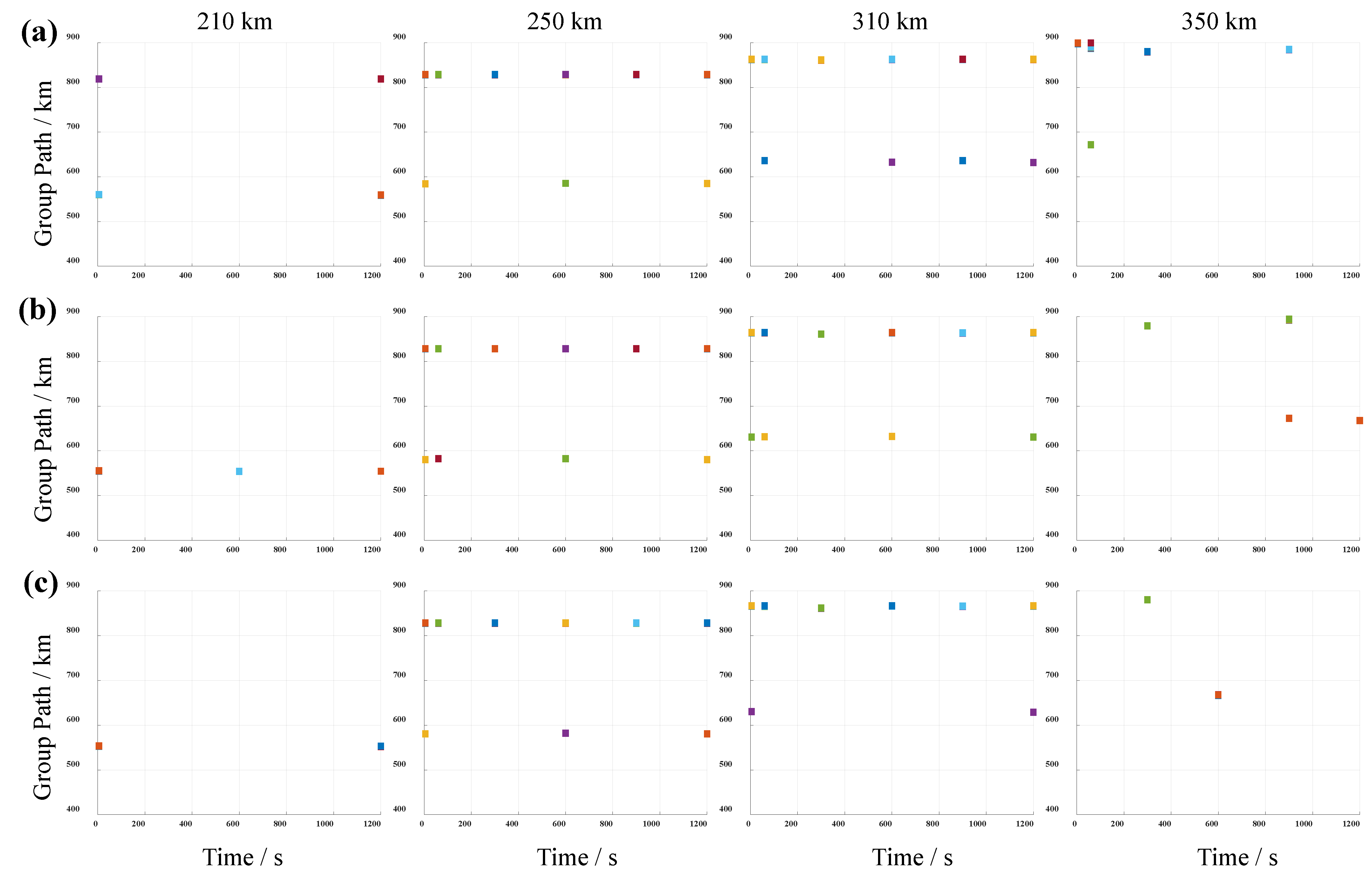
Figure 9 presents the group path–time evolution of received signals at ground-based receivers for barium release mass of 4 kg, 8 kg, and 12 kg. The echo signals are distinctly separable into two dominant components: (i) signals with group paths exceeding 800 km, attributable to reflection from the natural ionosphere or to composite reflection involving both the electron cloud and the natural ionosphere; and (ii) signals with group paths below 700 km, predominantly arising from direct reflection off the electron cloud. For a receiver at 210 km, the shielding time of the electron cloud formed by the 4 kg barium release is less than 1200 s, while the shielding times for the 8 kg and 12 kg releases are both longer than 1200 s. For receivers within the range of 250 km to 310 km, the natural ionosphere reflection signals with a group path of approximately 800 km can be stably received; at the same time, the signals with a group path of approximately 600 km mainly come from the reflection of the electron clouds, and this signal significantly evolves over time; the cloud generated by the 12 kg release has the longest impact duration on this channel. Further analysis reveals a positive correlation between the release mass and the disturbance duration: taking the receiver at 350 km as an example, the 12 kg release induces a pronounced disturbance in the channel with a group path of 900 km, and this disturbance persists for more than 1200 s.
Figure 9.
Group path–time diagrams for receivers at various ground positions for releases with different masses: (a) 4 kg, (b) 8 kg, and (c) 12 kg. All simulations assume a release altitude of 180 km, an ionization rate of 20%, a probing frequency of 12.8 MHz, and a transmitter position at −200 km.
3.3. Propagation Characteristics at Different Initial Ionization Rates
Due to the differences in release techniques employed in active release experiments, a fraction of barium atoms may already be ionized at the very beginning of the release, leading to a discrepancy between the initial number of barium ions and the total number of released barium atoms; this is referred to as the initial ionization rate. This section investigates the propagation characteristics of the artificial electron cloud for an initial ionization rate of 20% and 80%.
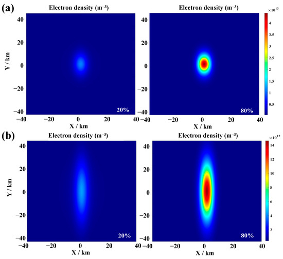
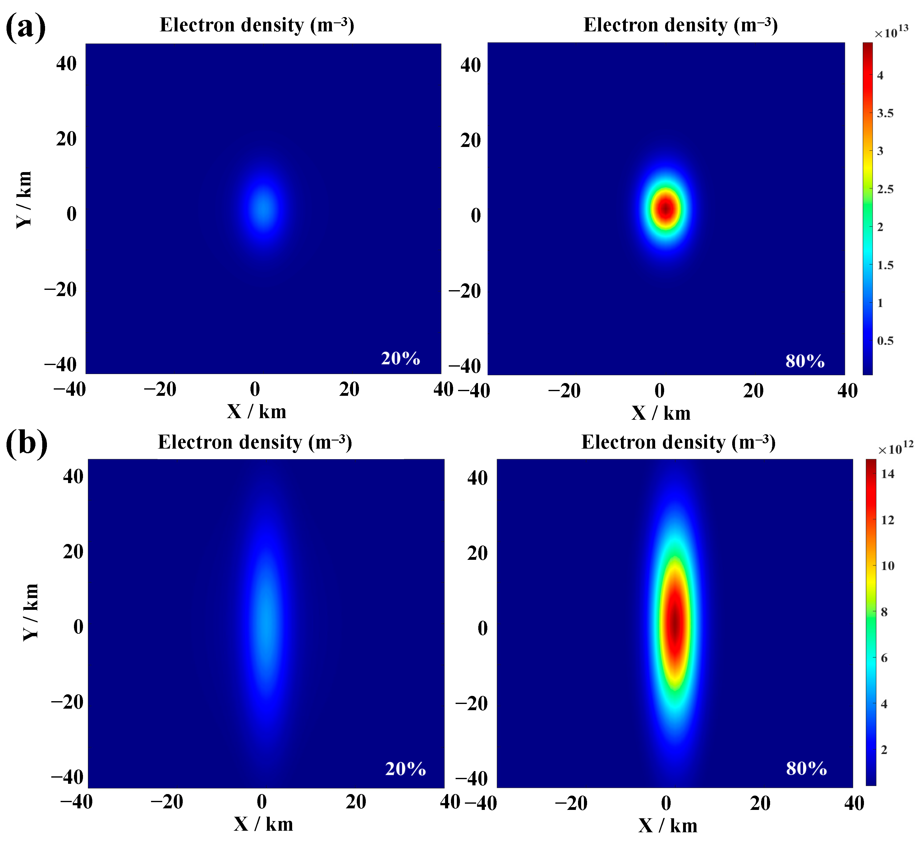
The spatial distribution of electron density of the artificial cloud at 60 s and 600 s for initial ionization rates of 20% and 80% is shown in Figure 10. It is important to note that the artificial electron cloud arises from two distinct physical sources: (i) a high-density core region formed by ionization occurring during the initial release phase, and (ii) peripheral electron contributions from the continuous ionization of the neutral barium cloud during subsequent evolution. At higher initial ionization rates, the resulting electron cloud is more concentrated in the initial release area, exhibiting a more localized spatial distribution with a significantly steeper radial density gradient. This enhances the plasma pressure gradient-driven effect along the geomagnetic field, leading to accelerated field-aligned expansion, increased cloud stretching, and more rapid growth in the long-axis scale. Concurrently, the early ionization of a large fraction of neutral barium atoms effectively mitigates loss due to subsequent oxidation reactions, resulting in higher electron yields, greater peak electron density of the cloud, and an extended overall lifetime.
Figure 10.
Morphological distribution of artificial electron clouds for initial ionization rates of 20% and 80% at a release altitude of 180 km and a mass of 10 kg: (a) 60 s after release; (b) 600 s after release.
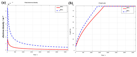
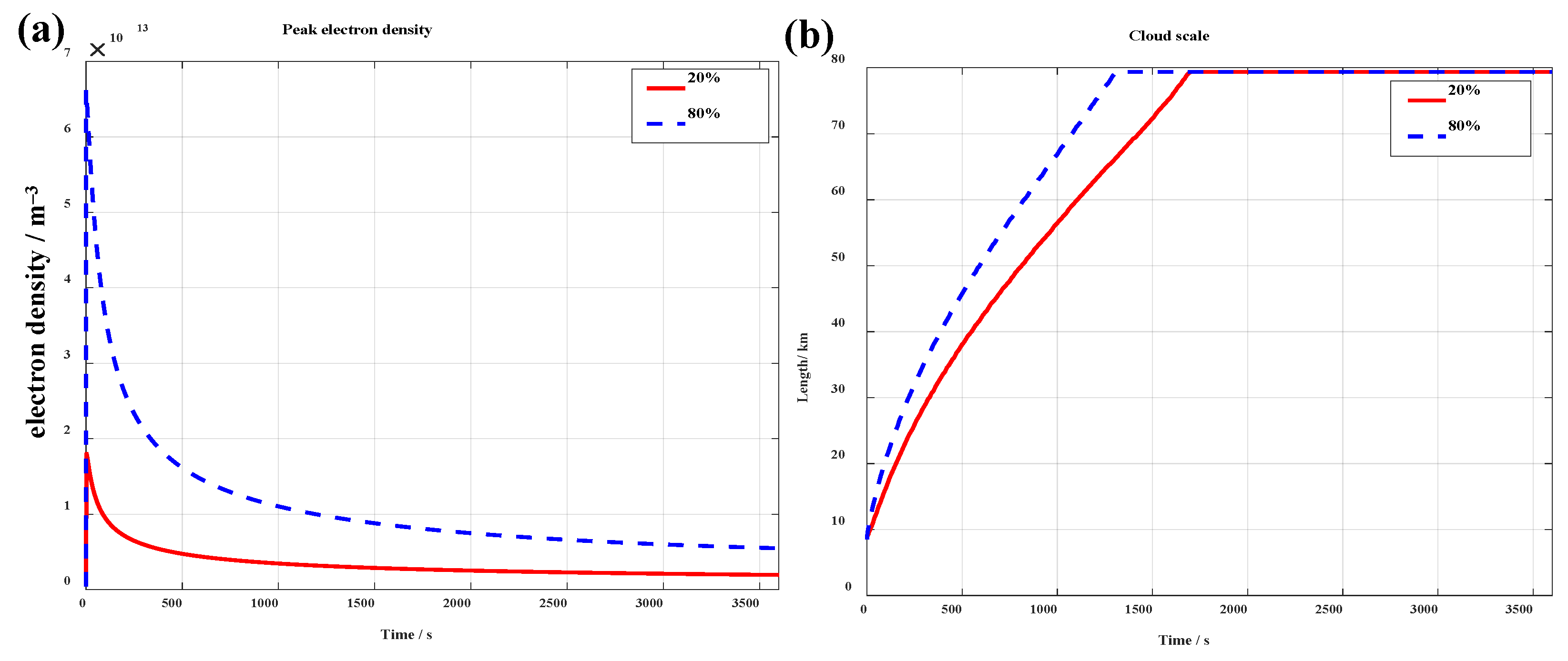
Figure 11 shows the evolution of peak electron density and cloud scale over time under different initial ionization rates. As previously mentioned, an increase in the initial ionization rate leads to a reduction in oxidation loss, significantly enhancing the peak electron number density of the artificial electron cloud: when the initial ionization rate is 20% and 80%, the corresponding maximum number density of the artificial electron cloud is 1.80 × 10¹³ m–3 and 6.63 × 10¹³ m–3, respectively. At the same time, a higher density gradient causes the barium cloud to stretch along the magnetic field direction at a faster rate, with the cloud scale (especially along the magnetic field lines) rapidly expanding, accompanied by a rapid decrease in electron number density. Over time, the difference in electron number density at the release center under different initial ionization rates will become smaller and smaller.
Figure 11.
Temporal evolution of (a) peak electron density and (b) cloud scale for initial ionization rates of 20% and 80%, with release altitude of 180 km and mass of 10 kg.
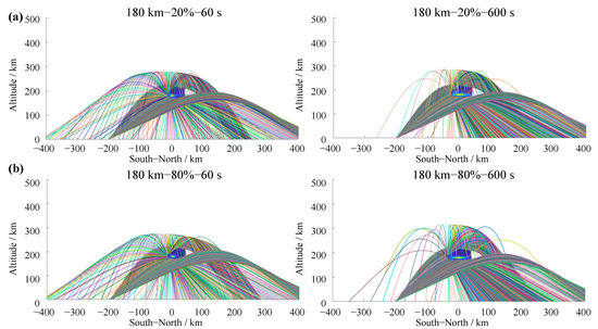
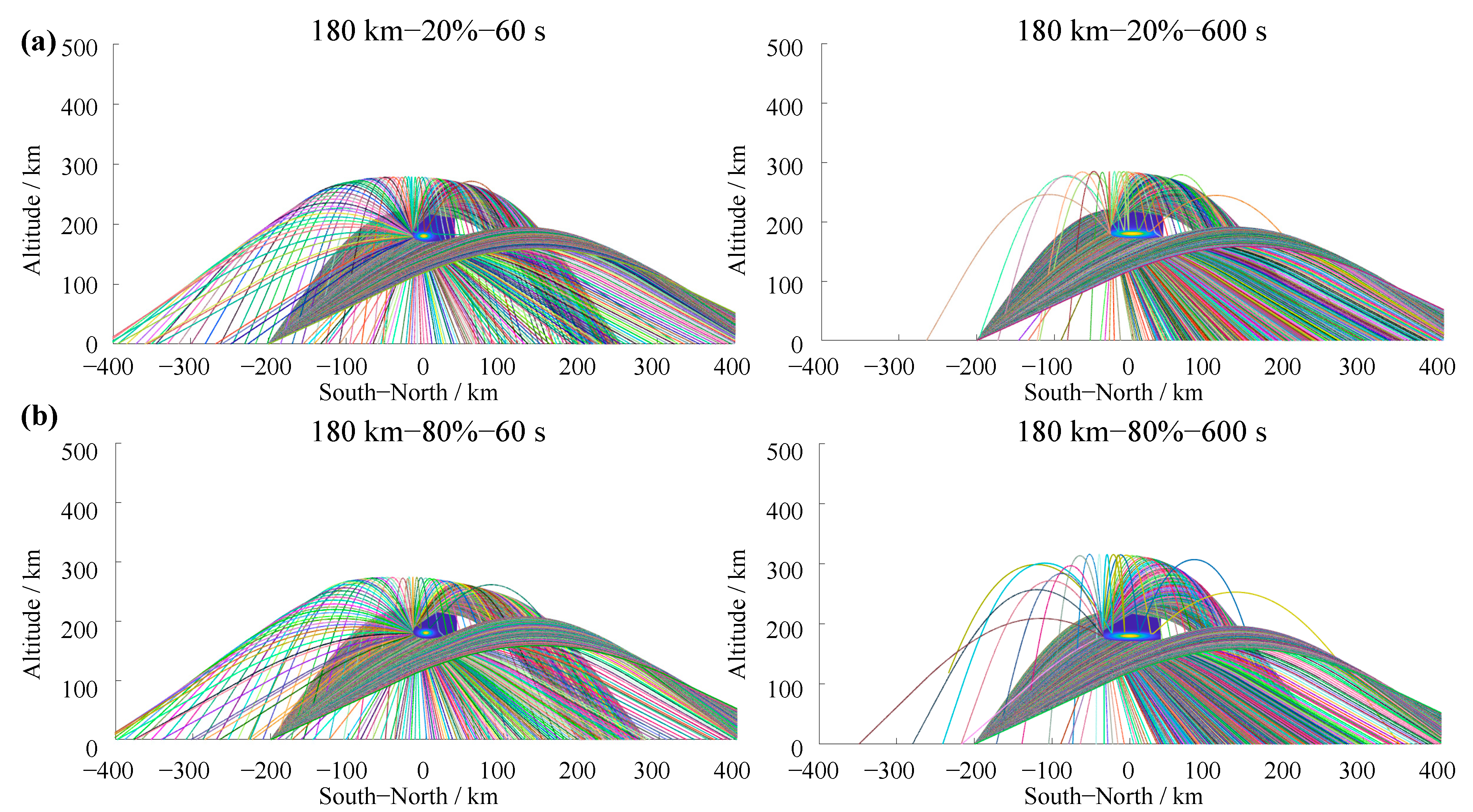
The ray-tracing results of the cloud at 60 s and 600 s for initial ionization rates of 20% and 80% are presented in Figure 12. Notably, the ray-tracing outcomes exhibit no significant discrepancies across the two ionization rates. At 60 s, the cloud retains an approximately spherical morphology with low overall curvature and a relatively uniform reflective surface, giving rise to abundant back-scattering signals. However, due to differences in cloud density and spatial extent, the ground-based signal shadow zone shows distinct variations in both range and location between the two cases. At 60 s after release, raising the initial ionization rate from 20% to 80% expands the signal enhancement zone from 55 km to 90 km, while simultaneously reducing the shadow-zone width from 158 km to 118 km. By 600 s, the cloud has undergone field-aligned stretching, leading to an expanded signal shadow zone and a marked reduction in back-scattering signals.
Figure 12.
Ray-tracing results for different initial ionization rates of 20% and 80%. All cases assume an altitude of 180 km, release mass of 10 kg, operating frequency of 10.8 MHz, and the transmitter located 200 km south of the cloud’s ground projection: (a) 60 s after release; (b) 600 s after release.
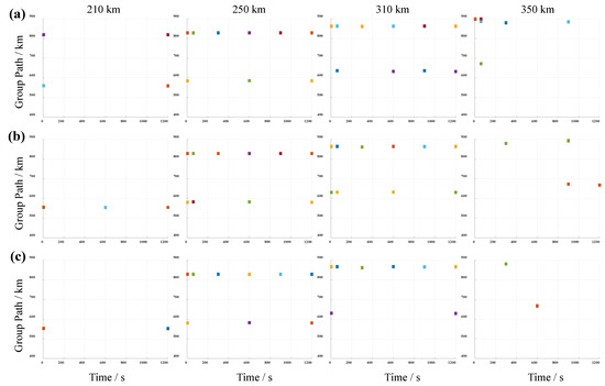
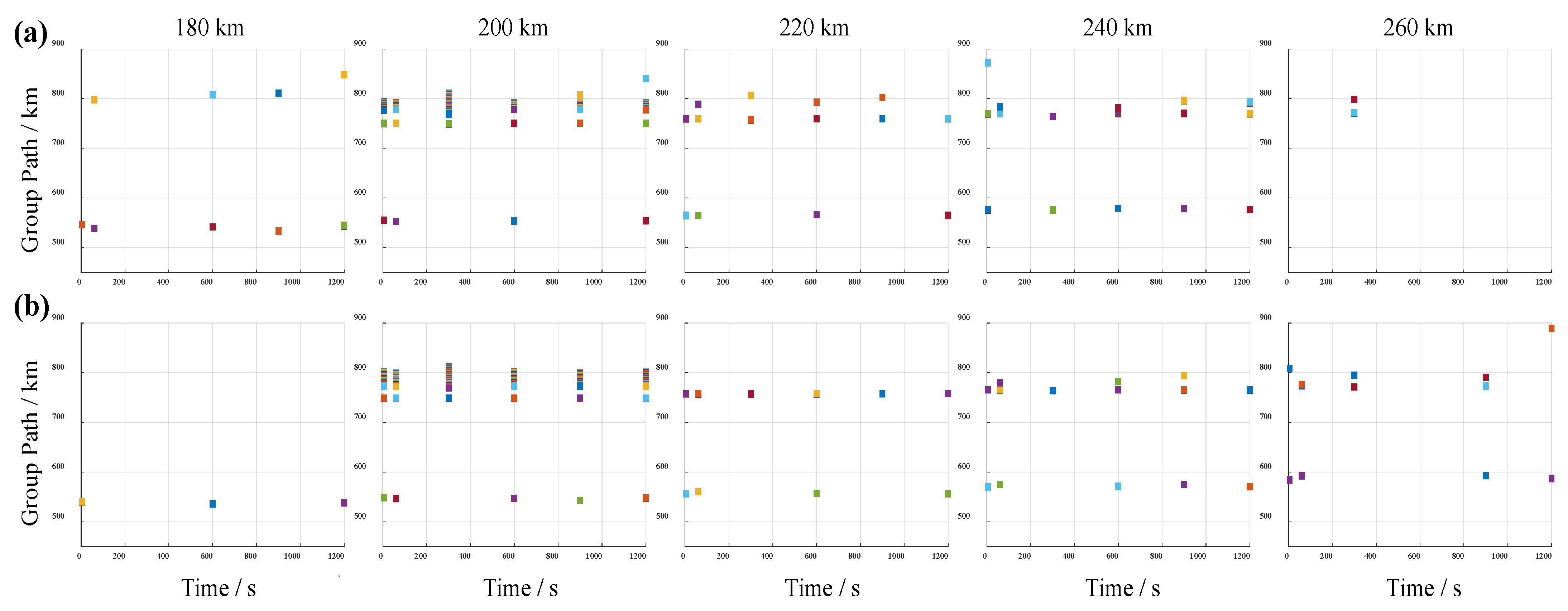
Figure 13 illustrates the group path–time evolution of signals received by the ground-based receiver under initial ionization rates of 20% and 80%. At an ionization rate of 20%, the group path channel of receivers located between 180 km and 240 km remains relatively stable, where stability is defined as the condition that the received signal amplitude does not fall below 30% of the background level for a continuous period of 600 s. Conversely, signals from receivers north of 260 km are significantly attenuated because the cloud occludes the propagation path. When the ionization rate is 80%, the signal enhancement region emerges within the range of approximately 200 km to 260 km, and the signal shadow zone shifts further north—consistent with the findings presented in Figure 13. At lower ionization rates, the signal channel for receivers spanning 180–240 km maintains long-term stability, with minimal cloud-induced interference. This behavior stems from the free diffusion of abundant neutral species associated with low ionization rates, which slows cloud-scale growth and density decay, promotes uniform energy distribution, and results in negligible temporal variations in scattering effects. In contrast, high ionization rates lead to steep cloud density gradients, rapid stretching along magnetic field lines, fast scale expansion, and swift peak density attenuation. Although the effective scattering region is large, the per-unit-volume scattering efficiency declines rapidly, rendering the spatial position of the shielding zone highly time-sensitive. Overall, low ionization rates yield gradual changes in cloud density and scale, facilitating stable signal coverage or controlled shielding (in this study, “signal coverage” encompasses both the shadow zone and the enhancement zones on its flanks, which together characterize the spatial extent of the cloud’s electromagnetic influence on the ground). High ionization rates, by contrast, induce rapid cloud stretching and accelerated density evolution, making them suitable for applications requiring fast communication response or localized intense signal suppression.
Figure 13.
Group path–time diagrams for receivers at various ground positions for different ionization rates: (a) 20% and (b) 80%. All cases assume an altitude of 180 km, release mass of 10 kg, operating frequency of 10.8 MHz, and the transmitter located 200 km south of the cloud’s ground projection.
3.4. Summary of Propagation Indicators
To facilitate cross-comparison of the propagation effects under different release conditions, Table 3 summarizes the key quantitative indicators for all simulation cases examined in Section 3.1, Section 3.2 and Section 3.3. The reported quantities include the peak electron density (Ne_max), cloud scale (defined as the 1/e width of the density contour for the altitude cases, and as the extent of the region with density exceeding 1012 m−3 for the mass cases), shadow-zone width, enhancement-zone width, and multipath delay spread. Unless otherwise noted, the values for cloud scale, shadow-zone width, enhancement-zone width, and multipath delay spread are taken at 300 s after release.
Table 3.
Summary of key propagation indicators of artificial electron cloud under different release conditions.
Table 3 clearly shows that increasing the release altitude enlarges the cloud scale and shadow-zone width while reducing the enhancement-zone width, and causing the multipath delay spread to increase. A larger release mass elevates the peak electron density, widens the shadow zone, and narrows the enhancement zone, reflecting stronger scattering and occlusion. A higher initial ionization rate produces a denser and more stretched cloud, resulting in a broader enhancement zone but a slightly reduced shadow-zone width at 300 s. These quantitative trends provide a direct reference for selecting release parameters according to specific application requirements.
To assess the robustness of our results against numerical parameters, we performed sensitivity tests on ray density (elevation sampling step: π/2048, π/4096, π/8192), the ray integration step (0.01 km, 0.05 km, 0.10 km), receiver acceptance radius (±0.5 km, ±1 km, ±2 km), and cloud grid spacing (0.5 km, 1 km), using the baseline case (180 km, 10 kg, 20%, 300 s). As detailed in the Supplementary Materials, varying the ray density (Figure S1) and integration step (Figure S2) changes the shadow-zone and enhancement-zone widths by less than 5% and 10%, respectively. The receiver acceptance radius (Table S1) primarily affects the multipath delay spread (90.6–240.8 km) due to path diversity, while the zone widths remain stable (164–172 km); we adopted ±1 km as a conservative choice. Refining the cloud grid from 1 km to 0.5 km (Figure S3) alters peak density by 2.8% and zone widths by less than 4%. These tests confirm that our main conclusions are robust with respect to numerical discretization and ray-tracing settings.
4. Conclusions
This paper integrates a two-fluid model with ray tracing to establish an analytical framework connecting release parameters, cloud morphology, and HF propagation characteristics. The influence of release altitude, mass, and the ionization rate is systematically examined.
With the increase in release altitude (150–210 km), the shadow-zone width rises from 116 km to 170 km, while its center shifts leftward (from 412 km to 253 km); at lower altitudes, collisional dominance produces a compact, high-density cloud that acts as a wide-angle scatterer, yielding extended ground echoes but a narrower shadow zone. Meanwhile, at higher altitudes, enhanced geomagnetic constraint induces field-aligned stretching that broadens the shadow zone and increases multipath delay, although the concurrent rapid density decay weakens the overall scattering intensity. With the increase in release mass (4 kg, 8 kg and 12 kg), the shadow-zone width grows monotonically, attaining 144 km, 158 km, and 174 km, respectively. Larger masses elevate the peak electron density and scattering strength, thereby widening the affected region and prolonging the disturbance. The increase in the initial ionization rate from 20% to 80% expands the signal enhancement zone from 55 km to 90 km, while simultaneously reducing the shadow-zone width from 158 km to 118 km; a high ionization rate suppresses oxidative losses and generates steep density gradients that drive rapid field-aligned expansion, which favors fast-response or local-suppression applications; while a low ionization rate results in gradual changes in cloud density and scale that facilitate stable coverage or controllable shielding effects.
Overall, the proposed analytical framework enables effective prediction of the electromagnetic response of artificial electron clouds under diverse release conditions, and clarifies the qualitative regulatory laws of release parameters on multipath structure, coverage range, and communication duration. Nevertheless, the model relies on several simplifying assumptions whose validity should be noted. The static point-source release serves as a useful baseline configuration that captures the essential physics of cloud formation and propagation; while extended release geometries could in principle be approximated by superposition of multiple point sources, the validity of such an approach for interacting clouds would require separate verification due to the nonlinear nature of the plasma model. The constant photoionization rate, simplified barium chemistry (neglecting the reaction between Ba and atomic oxygen), and perturbative treatment of ion inertia are all well justified for the F region altitudes (150–210 km) and short timescales (≤1 h) considered here. Additionally, the geomagnetic field is treated as constant, which is appropriate for the localized (≤a few hundred km) and short-term (≤1 h) disturbances modeled. The boundary conditions for the plasma cloud model employ a constant-value extrapolation scheme, which is justified when the density gradient at the boundaries is small. Moreover, the ionosphere exhibits pronounced spatiotemporal variability driven by solar activity, local time, geomagnetic conditions, and seasonal cycles [38,39,40]. Future work will incorporate realistic neutral atmospheric dynamics, full-wave solvers, and time-varying background ionospheric conditions to refine mission-specific predictions.
Supplementary Materials
The following supporting information can be downloaded at: https://www.mdpi.com/article/10.3390/eng7080369/s1, Figure S1: Ray-tracing results under different elevation sampling steps; Figure S2: Ray-tracing results under different ray integration step sizes; Figure S3: Ray-tracing results under different cloud spatial grid spacing; Table S1: Sensitivity test of calculation results under different ray densities, integration step sizes, receiver ranges and cloud cluster grid step sizes.
Author Contributions
Conceptualization, X.Z. and Y.H.; methodology, X.Z. and Y.H.; software, X.Z.; validation, X.Z.; formal analysis, L.D. and Y.H.; investigation, L.D. and Y.H.; resources, X.Z.; data curation, X.Z.; writing—original draft preparation, X.Z.; writing—review and editing, X.Z., L.D. and Y.L.; visualization, Y.L.; supervision, Y.H.; project administration, X.Z.; funding acquisition, X.Z., Y.L. and L.D. All authors have read and agreed to the published version of the manuscript.
Funding
This research was funded by the Science and Technology Department of Hubei Province (Grant No. 2023AFB441; No. 2025AFB344), the National Natural Science Foundation of China (Grant No. 42104028), and the Hubei Provincial Department of Education (Grant No. Q20244501).
Institutional Review Board Statement
Not applicable.
Informed Consent Statement
Not applicable.
Data Availability Statement
The background atmosphere, ionosphere, and magnetic field data were download from the NRLMSIS 2.1 atmosphere model (https://kauai.ccmc.gsfc.nasa.gov/instantrun/nrlmsis/) (accessed on 20 August 2025), IRI-2020 ionospheric model (https://kauai.ccmc.gsfc.nasa.gov/instantrun/iri/) (accessed on 20 August 2025), and DGRF/IGRF 1945–2030 (IGRF-14) magnetic field model (https://ccmc.gsfc.nasa.gov/modelweb/models/igrf_vitmo.php (accessed on 20 August 2025)), respectively. Typical artificial electron cloud density distribution data (release altitude: 180 km; payload mass: 10 kg; initial ionization rate: 20%) is provided as Supplementary Materials. Other data are available from the corresponding author upon reasonable request.
Conflicts of Interest
The authors declare no conflicts of interest.
Abbreviations
The following abbreviations are used in this manuscript:
| HF | High frequency |
| VHF | Very high frequency |
| OTHR | Over-the-horizon radar |
| Ba | Barium |
| GTD | Geometrical theory of diffraction |
Appendix A. Model Validation
Figure A1.
Velocity distributions of barium ions (Ba+) 2 s after release, parallel to the magnetic field direction (x–z panel) and perpendicular to the magnetic field direction (x–y panel), the length of the arrows in the figure indicates the magnitude of the speed, and the direction of the arrows represents the direction of the speed. (a) Ma and Schunk, 1993 [29]; (b) simulation results of our model.
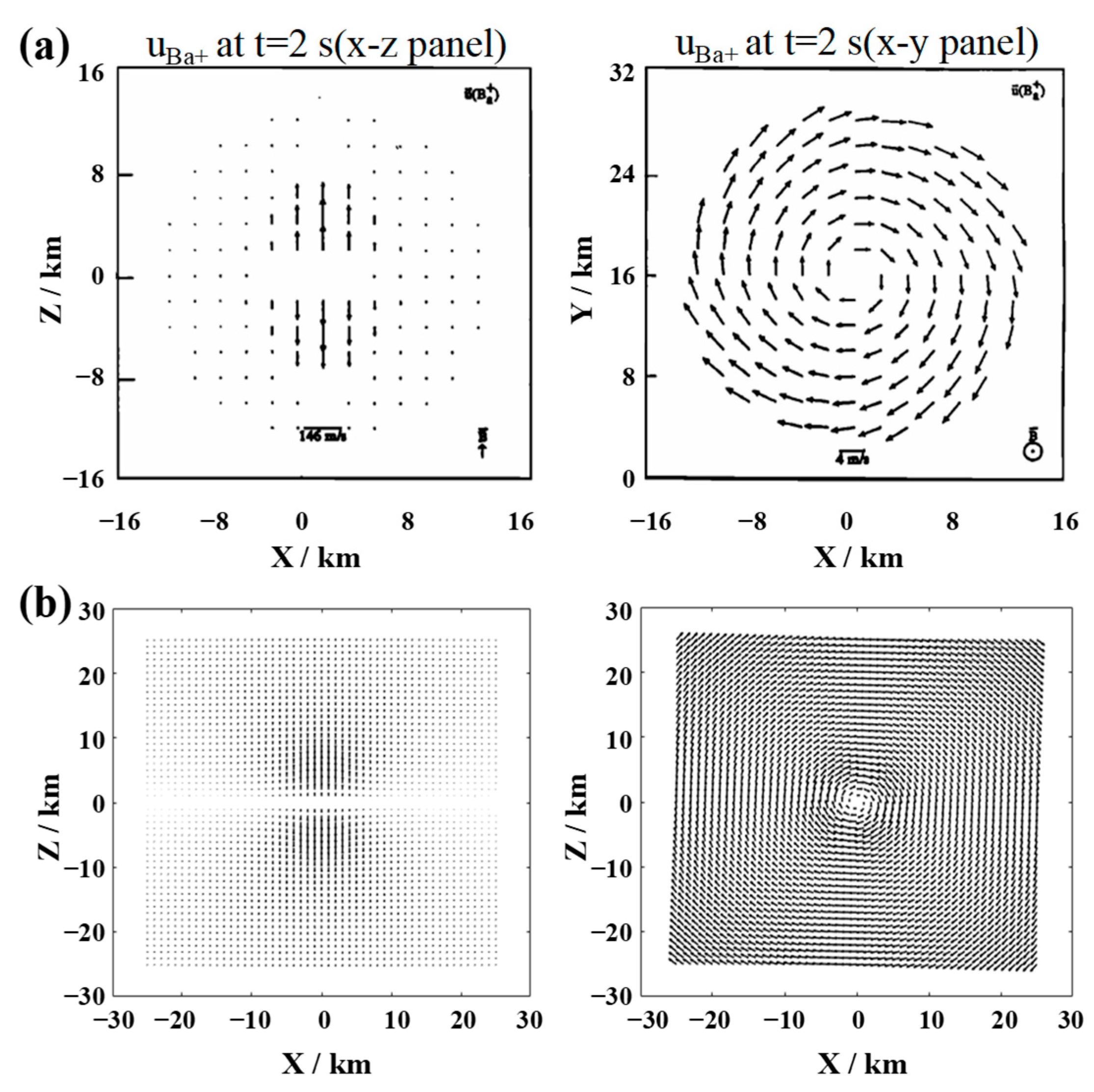
Figure A2.
Velocity distributions of oxygen ions (O+) 2 s after release, parallel to the magnetic field direction (x–z panel) and perpendicular to the magnetic field direction (x–y panel), the length of the arrows in the figure indicates the magnitude of the speed, and the direction of the arrows represents the direction of the speed. (a) Ma and Schunk, 1993 [29]; (b) simulation results of our model.
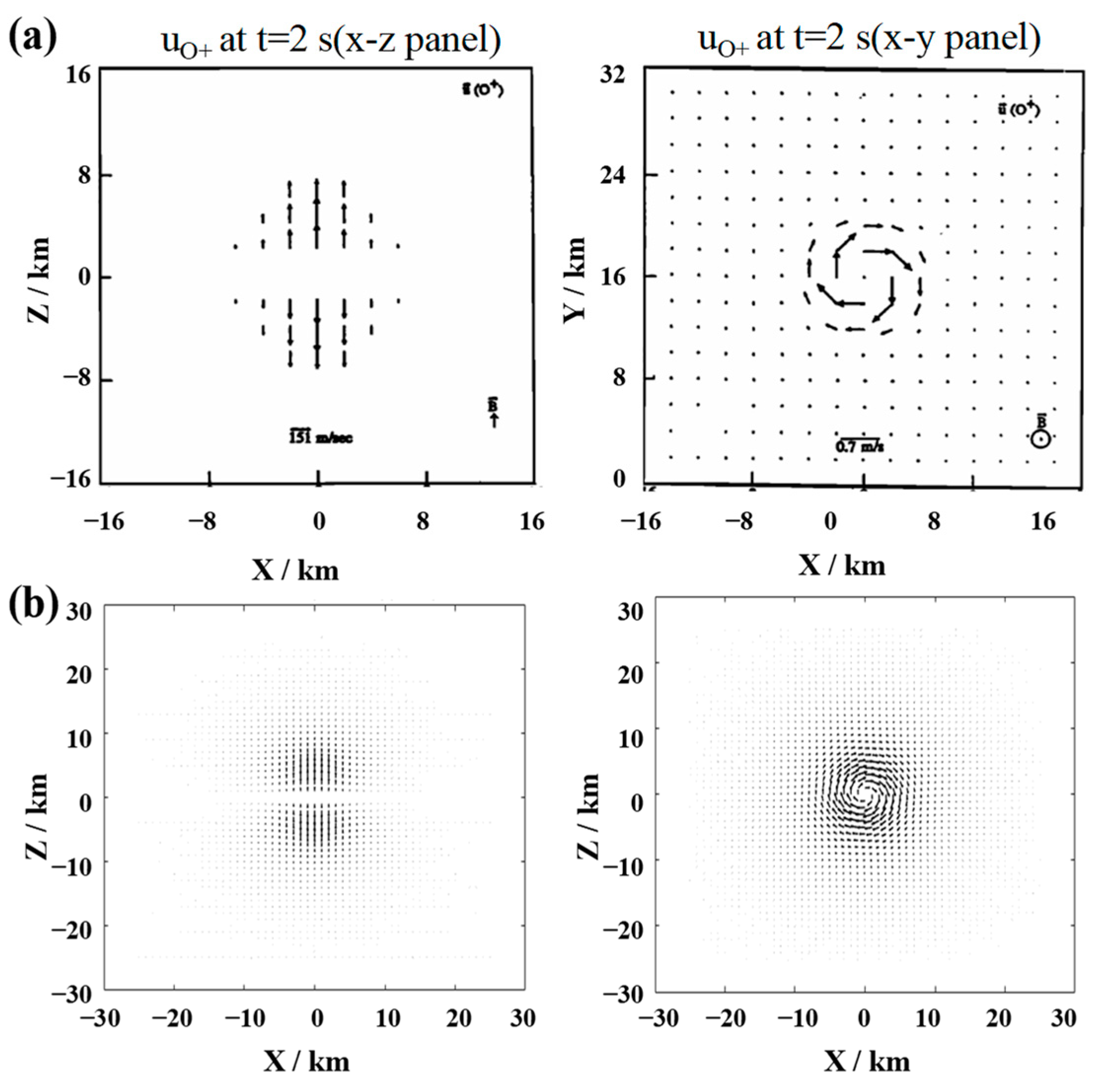
Figure A3.
Comparison of the density distribution of Ba+ (top) and O+ (bottom) at t = 1 s. Left panel: simulation results calculated by our model; right panel: simulation results calculated by Xie L., 2013 [32]. In the right panel, [R] = 100 km, and all units are cm–3.
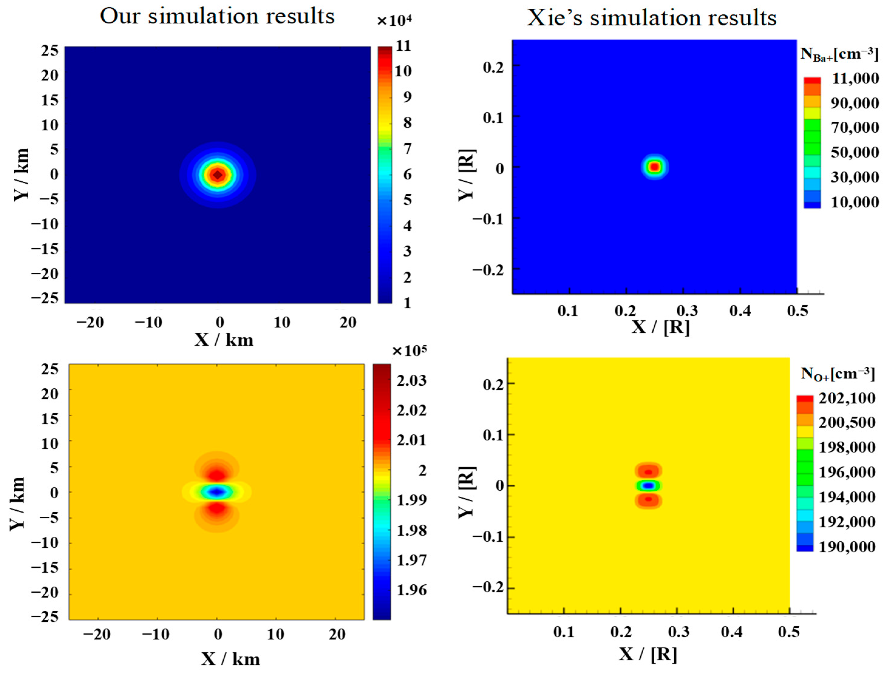
Figure A4.
Comparison of the density distribution of Ba+ (top) and O+ (bottom) at t = 5 s. Left panel: simulation results calculated by our model; right panel: simulation results calculated by Xie L., 2013 [32]. In the right panel, [R] = 100 km, and all units are cm–3.
References
- Frazer, G.J.; Williams, C.G. Emerging trends in radar: HF skywave radar. IEEE Aerosp. Electron. Syst. Mag. 2025, 40, 78–82. [Google Scholar] [CrossRef] [Scilit]
- Ji, X.; Li, J.; Yang, Q. Annual characteristic analysis of ionosphere reflection from middle-latitude HF over-the-horizon radar in the northern hemisphere. IEEE Trans. Geosci. Remote Sens. 2023, 61, 5104117. [Google Scholar] [CrossRef] [Scilit]
- Frissell, N.A.; Vega, J.S.; Markowitz, E.; Gerrard, A.J.; Engelke, W.D.; Erickson, P.J.; Miller, E.S.; Luetzelschwab, R.C.; Bortnik, J. High Frequency Communications Response to Solar Activity in September 2017 as Observed by Amateur Radio Networks. Space Weather 2019, 17, 118–132. [Google Scholar] [CrossRef] [Scilit]
- Ankita, M.; Tulasi Ram, S.; Ajith, K.K.; Sripathi, S. Deep electron density depletion near sunset terminator on St. Patrick’s Day storm and its impacts on Skywave propagation. Space Weather 2023, 21, e2022SW003369. [Google Scholar] [CrossRef] [Scilit]
- Khaled, K.; El Sayed Ahmad, A.; Pagani, P.; Fleury, R. A Study on the Influence of Solar Flares on High Frequency Radio Propagation. IEEE Open J. Antennas Propag. 2025, 13, 35–48. [Google Scholar] [CrossRef]
- Davis, T.N. Chemical releases in the ionosphere. Rep. Prog. Phys. 1979, 42, 1565. [Google Scholar] [CrossRef] [Scilit]
- Gao, J.F.; Guo, L.X.; Xu, Z.W.; Zhao, H.S.; Feng, J. Simulation and analysis of chemical release in the ionosphere. Adv. Space Res. 2018, 61, 2234–2244. [Google Scholar] [CrossRef] [Scilit]
- Gao, J.F.; Xu, Z.W.; Guo, L.X.; Xue, K.; Zhao, H.S. Controlling Factors of Artificial Irregularities Triggered by Chemical Release at Low Latitude Ionosphere. Space Weather 2023, 21, e2022SW003229. [Google Scholar] [CrossRef] [Scilit]
- Zhu, X.; Hu, Y.; Deng, L.; Zhao, Z. Numerical investigation of artificial electron clouds generated by alkali metal release in near-space. Earth Planets Space 2026, 78, 23. [Google Scholar] [CrossRef] [Scilit]
- Rosenberg, N.W. Chemical releases in the upper atmosphere (Project Firefly), A summary report. J. Geophys. Res. 1963, 68, 3057–3063. [Google Scholar] [CrossRef] [Scilit]
- Reasoner, D.L. Chemical-release mission of CRRES. J. Spacecr. Rocket. 1992, 29, 580–584. [Google Scholar] [CrossRef] [Scilit]
- Bernhardt, P.A.; Roussel-Dupre, R.A.; Pongratz, M.B.; Haerendel, G.; Valenzuela, A.; Gurnett, D.A.; Anderson, R.R. Observations and theory of the AMPTE magnetotail barium releases. J. Geophys. Res. 1987, 92, 5777. [Google Scholar] [CrossRef] [Scilit]
- Caton, R.; Pederson, T.; Groves, K.; Hines, J.; Cannon, P.S.; Jackson-Booth, N.; Parris, R.T.; Holmes, J.M.; Su, Y.-J.; Mishin, E.V.; et al. Artificial ionospheric modification: The Metal Oxide Space Cloud experiment. Radio Sci. 2017, 52, 539. [Google Scholar] [CrossRef] [Scilit]
- Pongratz, M.B. History of Los Alamos Participation in Active Experiments in Space. Front. Phys. 2018, 6, 144. [Google Scholar] [CrossRef] [Scilit]
- Zhao, H.-S.; Feng, J.; Xu, Z.-W.; Wu, J.; Wu, Z.-S.; Xu, B.; Xue, K.; Xu, T.; Hu, Y.-L. A temporal three-dimensional simulation of samarium release in the ionosphere. J. Geophys. Res. Space Phys. 2016, 121, 10508–10519. [Google Scholar] [CrossRef] [Scilit]
- Zhao, H.S.; Feng, J.; Xu, Z.W.; Liu, Y.-X.; Xue, K.; Wu, J.; Wang, C.; Xie, S.-Z.; Peng, H.-Y. Enhancement of ionospheric heating effect by chemical release. Sci. Rep. 2024, 14, 13234. [Google Scholar] [CrossRef] [Scilit] [PubMed]
- Fletcher, A.C.; Crabtree, C.; Ganguli, G.; Siefring, C.; Soto-Chavez, A.R.; Netwall, C. Rocket-Released Neutral Clouds in the Ionosphere: Formation, Evolution, and Detection. J. Geophys. Res. Space Phys. 2023, 128, e2022JA031039. [Google Scholar] [CrossRef] [Scilit]
- Yokoyama, Y.; Tima, S. Unexpected strong parallel electric field at the lower E region observed during a barium release experiment. In Proceedings of the EGU General Assembly, Vienna, Austria, 27 April–2 May 2025. [Google Scholar] [CrossRef] [Scilit]
- Xie, S.Z.; Zhao, H.S.; Xu, Z.W.; Ren, G.L.; Wang, C.; Ge, S.C. Refined modeling and propagation characteristics for the space plasma cloud. Chin. J. Radio Sci. 2024, 39, 56–64. [Google Scholar] [CrossRef]
- Marmo, F.F.; Engelman, A. Artificial ionospheres for communications. IRE Trans. Mil. Electron. 1960, 4, 270–284. [Google Scholar] [CrossRef] [Scilit]
- Minkwitz, D.; Borries, C.; Rother, M. Ray tracing methods for wave propagation in anisotropic, inhomogeneous, and time-varying ionosphere: State-of-the-art overview. Adv. Radio Sci. 2021, 19, 41–53. [Google Scholar] [CrossRef] [Scilit]
- Joshi, D.; Groves, K.M.; Mcneil, W.; Carrano, C.; Caton, R.G.; Parris, R.T. Hf propagation results from the metal oxide space cloud (mosc) experiment. Radio Sci. 2017, 52, 710. [Google Scholar] [CrossRef] [Scilit]
- Xie, S.; Ren, G.; Xue, K.; Zhao, H.; Xu, Z.; Zheng, Y. HF Propagation Effects Caused by Artificial Plasma Cloud in the Ionosphere. In Proceedings of the 13th International Symposium on Antennas, Propagation and EM Theory, Zhuhai, China, 1–4 December 2021. [Google Scholar] [CrossRef] [Scilit]
- Ma, X.; Fang, H.; Wang, S.; Chang, S. Impact of the Ionosphere Disturbed by Rocket Plume on OTHR Radio Wave Propagation. Radio Sci. 2021, 56, e2020RS007183. [Google Scholar] [CrossRef] [Scilit]
- Zhao, H.S.; Xu, Z.W.; Tang, W. Electromagnetic scattering by artificial plasma clouds in the ionosphere. IEEE Trans. Antennas Propag. 2020, 68, 4810. [Google Scholar] [CrossRef] [Scilit]
- Zhu, X.; Hu, Y.; Zhao, Z.; Ni, B.; Zhang, Y. Ionospheric disturbance caused by artificial plasma clouds under different release conditions. Earth Planets Space 2020, 72, 183. [Google Scholar] [CrossRef] [Scilit]
- Rosenberg, N.W.; Best, G.T. Chemistry of barium released at high altitudes. J. Phys. Chem. 1971, 75, 1412–1418. [Google Scholar] [CrossRef] [Scilit]
- Li, L.; Xu, R.L. Neutral barium cloud evolution at different altitudes. Chin. Phys. Lett. 2002, 19, 1214–1216. [Google Scholar] [CrossRef] [Scilit]
- Ma, T.Z.; Schunk, R.W. Ionization and expansion of barium clouds in the ionosphere. J. Geophys. Res. 1993, 98, 323–336. [Google Scholar] [CrossRef] [Scilit]
- Hu, Y.; Zhao, Z.; Zhang, Y. Ionospheric disturbances produced by chemical releases and the resultant effects on short-wave ionospheric propagation. J. Geophys. Res. 2011, 116, A07307. [Google Scholar] [CrossRef] [Scilit]
- Ma, T.Z.; Schunk, R.W. Plasma cloud expansion in the ionosphere: Three-dimensional simulation. J. Geophys. Res. 1991, 96, 5793–5810. [Google Scholar] [CrossRef] [Scilit]
- Xie, L. Ionospheric Barium Cloud Release: Two-Component MHD Simulation and Experimental Observation. Doctoral Dissertation, University of Chinese Academy of Sciences, Beijing, China, 2013. [Google Scholar]
- Song, H.; Qing, H.; Zou, X. A parallel optimized 3D numerical ray tracing method for fast and accurate simulation of disturbed oblique ionograms. Adv. Space Res. 2022, 70, 2894–2904. [Google Scholar] [CrossRef] [Scilit]
- Ma, X.; Guo, P.; Wu, M. Simulation Research on the Influence of Plasma Bubbles on Radio Wave Propagation. Radio Sci. 2023, 58, e2022RS007577. [Google Scholar] [CrossRef] [Scilit]
- Jiang, X.; Li, H.; Guo, L. The propagation delay analysis of short-wave multipath based on the ionospheric ray-tracing homing-in algorithm. In Proceedings of the 2024 Cross Strait Radio Science and Wireless Technology Conference, Macao, China, 4–7 November 2024. [Google Scholar] [CrossRef] [Scilit]
- Jones, R.M.; Stephenson, J.J. A Versatile Three-Dimensional Ray Tracing Computer Program for Radio Waves in the Ionosphere; Report; U.S. Department of Commerce, Office of Telecommunications: Washington, DC, USA, 1975; pp. 75–76.
- Li, G.; Yang, S.; Liu, Y.; Nie, Z. A Variable Step Length Hybrid Approach for Electromagnetic Ray Tracing in Ionosphere. Electromagnetics 2007, 27, 331–340. [Google Scholar] [CrossRef] [Scilit]
- Lopez-Urias, C.; Vazquez-Becerra, G.E.; Nayak, K.; Lopez-Montes, R. Analysis of Ionospheric Disturbances during X-Class Solar Flares (2021–2022) Using GNSS Data and Wavelet Analysis. Remote Sens. 2023, 15, 4626. [Google Scholar] [CrossRef] [Scilit]
- Pandey, S.; Mishra, A.; Singh, V.; Kumar, S. Study of the thermosphere-ionosphere response to geomagnetic storm of April 2023. Indian J. Phys. 2026, 100, 2603–2611. [Google Scholar] [CrossRef] [Scilit]
- Nayak, K.; Carrillo-Vargas, A.; López Urias, C.; Romero-Andrade, R.; Cifuentes Nava, G.; Caccavari-Garza, A. Ionospheric response to the intense geomagnetic storm of May 10, 2024, in central Mexico. Adv. Space Res. 2025, 76, 7412–7432. [Google Scholar] [CrossRef] [Scilit]

Disclaimer/Publisher’s Note: The statements, opinions and data contained in all publications are solely those of the individual author(s) and contributor(s) and not of MDPI and/or the editor(s). MDPI and/or the editor(s) disclaim responsibility for any injury to people or property resulting from any ideas, methods, instructions or products referred to in the content. |
© 2026 by the authors. Licensee MDPI, Basel, Switzerland. This article is an open access article distributed under the terms and conditions of the Creative Commons Attribution (CC BY) license.