Mechanism Study of the Interaction Between Sloshing Water Flow and Elastic Baffles in a Shaking Tank

Abstract

In this study, we employ the SPH method to systematically investigate the mechanism of interaction between sloshing water flow and elastic baffles in a shaking tank from two perspectives: single and multiple elastic baffles. We focus on researching the influence of external excitation frequency $\omega$, shaking angle $\theta$, and immersion ratio $h/h_b$ on the free surface elevations of the sloshing, the displacements and forces of the elastic baffles’ top positions, and the impact pressures on the side wall of the shaking tank. The results illustrate that the free surface elevation fluctuation period of the sloshing exhibits a significant frequency dependence on $\omega$. Specifically, when $\omega$ approaches the resonant frequency of the tank ${\omega }_1$, the free surface elevations, displacements, forces, and impact pressures reach their maximum values. The shaking angle $\theta$ has a clear amplification effect for the free surface elevations, displacements, forces, and impact pressures. The amplitudes of the free surface elevations are relatively close when $h/h_b=0.75$ and $1.0$ and gradually decrease when $h/h_b=1.25$. The displacements, forces, and impact pressures show a decreasing trend with increasing $h/h_b$.

1. Introduction

Sloshing water flow, a phenomenon of water movement within liquid-storage tanks caused by external excitation, is common in both natural and engineering practices. Typical engineering practices include the sloshing in large reservoirs during earthquakes and in oil or liquefied natural gas transport vehicles. It is generally believed that when a container loaded with water is subjected to external excitation and the amplitude of the external excitation is large or the frequency is close to the resonant frequency of the container, the water inside the container will undergo a severe sloshing process, while applying severe hydrodynamic impact on the tank walls [1]. In other words, sloshing water flow will have a notable impact on the structural safety of the loading container itself. Taking the above engineering practices as an example, the motion of the sloshing in the reservoir during an earthquake may exert enormous impact pressure on the reservoir dam, causing structural instability and even damage to the reservoir dam body [2]; the sloshing in oil or liquefied natural gas transport vehicles may cause local rupture and overall instability of the vehicles, which may lead to oil spills and vehicle overturning [3]. Therefore, studying how to suppress the amplitude of the sloshing and reduce its impact on liquid-storage tanks has significant practical engineering implications.

Over the past few decades, researchers have found that installing baffles in liquid-storage tanks is an effective method for suppressing the amplitude of the sloshing. However, most relevant research currently focuses on rigid baffles that suppress the sloshing in a shaking tank. Cho and Lee [4] numerically investigated the large-amplitude sloshing of water flow in a two-dimensional shaking tank with rigid baffles under conditions of horizontal forced excitation. They found a clear dependence between the severity of the sloshing and the design parameters of the baffles. Akyildiz and Ünal [5] compared the impact pressure of the sloshing in a shaking tank with vertical rigid baffles and without baffles through experiments. They found that vertical rigid baffles can effectively reduce the impact pressure of the sloshing on the wall and suppress the amplitude of the sloshing. Liu and Lin [6] used the Large Eddy Simulation (LES) method to numerically investigate the sloshing in a three-dimensional shaking tank with rigid baffles. They found that vertical baffles were more effective than horizontal baffles in suppressing the amplitude of the sloshing and reducing the impact pressure of sloshing water on the wall. Xue et al. [7] and Chu et al. [8] investigated the influence of various shape configurations and multiple vertical rigid baffles on the motion response of the sloshing in a shaking tank through experiments. The results showed that installing vertical baffles can change the resonant frequency of the shaking tank. Nasar and Sannasiraj [9], as well as Yu et al. [10], conducted experimental research on the sloshing in a shaking tank containing a vertical rigid baffle. They concluded that the closer the baffle position is to the sloshing mode node, the more effective the amplitude suppression of the sloshing. Zang et al. [11] used the Boundary Element Model (BEM) to numerically investigate the interaction process between the sloshing and porous rigid baffles. They explored the influence of the baffle’s length and porosity on the amplitude of the sloshing. Overall, the research on the suppression of the sloshing by rigid baffles (namely, the interaction between the sloshing and rigid baffles) is relatively systematic and comprehensive, with abundant results.

With the development of fluid–structure interaction (FSI) numerical methods, researchers have begun to focus on suppressing the amplitude of the sloshing using elastic baffles. However, compared to rigid baffles, research results related to elastic baffles are rarely published. Paik et al. [12] employed a nonlinear finite element method coupled with a time-averaged Reynolds-averaged Navier–Stokes/separated vortex solver to numerically investigate the response characteristics of the free surface of the sloshing in a shaking tank with elastic baffles under oscillatory excitation conditions. Hwang et al. [13] employed the Moving Particle Simulation (MPS) method to numerically investigate the sloshing in a shaking tank under the conditions of no baffle, rigid baffle, and elastic baffle. They primarily investigated the damping effect of the aforementioned conditions on the amplitude of the sloshing. Considering the interaction between the sloshing and an elastic baffle, Maiti and Bhattacharyya [14] conducted experimental research on the amplitude and flow characteristics of the water flow around a cantilevered elastic baffle in a diamond-shaped shaking tank. Cho et al. [15] numerically solved the interaction between the sloshing and porous elastic baffles using Green’s function matching feature function expansion method. They explored the damping effect of baffle porosity and stiffness on the amplitude of the sloshing. Cao et al. [16] developed a semi-analytical solution method to numerically investigate the motion response of the sloshing in a two-dimensional shaking tank with dual elastic baffles. They primarily explored the influence of the elastic baffle’s parameters and horizontal excitation frequency on the amplitude of the sloshing. Ren et al. [17,18] employed the SPHinXsys numerical model, combined with experiments, to investigate the interaction between the sloshing and an elastic baffle. Specifically, they conducted systematic research on the free surface, pressure, and baffle deformation when the sloshing interacted with the elastic baffle. Although the above research has made some progress, there are still shortcomings in the understanding of the effectiveness of the interaction between elastic baffles and the sloshing. The most prominent issue is the lack of exploration on the intrinsic relationship between the resonant frequency of the shaking tank and the motion response of the sloshing and elastic baffles. Additionally, research on the mechanism of interaction between the sloshing and elastic baffles in a shaking tank is rare.

In recent years, the Smoothed Particle Hydrodynamics (SPH) method has undergone rapid development due to its superior ability to capture large deformations, handle free surfaces, and move boundaries. Researchers have widely applied it in many FSI-related scientific issues [17,19,20]. Given the advantages of the SPH method in addressing FSI problems and the shortcomings of the aforementioned research, this paper aims to utilize the SPH method to systematically investigate the mechanism of interaction between the sloshing and elastic baffles in a shaking tank. Despite recent advancements in SPH and FSI modeling, critical gaps remain in fully understanding the hydro-elastic interactions between sloshing fluids and elastic baffles. Previous numerical studies (e.g., Hwang et al. [13]; Ren et al. [17,18]) have primarily focused on standard shaking tanks or single-baffle configurations without deeply examining the frequency-dependent resonance behaviors. Specifically, the intrinsic correlation between the shaking tank’s resonant frequency and the coupled dynamic response of multiple elastic baffles remains largely unexplored.

To explicitly address this gap, the present study distinguishes itself from previous FSI research by systematically investigating the hydro-elastic damping mechanisms of both single and multiple elastic baffles in a shaking tank using an improved SPH model. Rather than merely reporting the suppression effects, we focus on the frequency-matching mechanism—correlating external excitation frequencies with the tank’s first-order resonant frequency—to reveal how dynamic structural deformation and multi-baffle configurations actively modulate fluid resonance.

2. Methodology

2.1. SPH Method

The SPH method utilizes integral equations based on interpolation or weighting functions to transform the conservation laws of continuum fluid mechanics from a partial differential form to a form suitable for particle simulation. This interpolation or weighting function is commonly referred to as a kernel function. Based on the kernel function, we can write the expression for the general function ${\mathit{f}}_a=\mathit{f}\left({\mathit{x}}_a\right)$ at any particle a as

$${\mathit{f}}_a={\sum }_b{\displaystyle \frac{m_b}{{\rho }_b}}{\mathit{f}}_{b}W\left({\mathit{x}}_a-{\mathit{x}}_b,\Gamma \right),$$

(1)

where the subscript “a” represents any particle a, and the subscript “b” represents any adjacent particle of that particle; $m$ is the particle mass; $\rho$ is the particle density; ${\mathit{x}}_a$ and ${\mathit{x}}_b$ are the spatial coordinate systems of particles a and b; $\Gamma$ is the smoothing length of the kernel function, $\Gamma =\sqrt{2}\Delta l$; and $\Delta l$ is the initial particle spacing.

$W\left(\mathit{x},\Gamma \right)$ is the kernel function, and the expression of it can be expressed as

$$W\left(\mathit{x},\Gamma \right)={\beta }_D{\left(1-{\displaystyle \frac{q}{2}}\right)}^4(2q+1) 0\le q\le 2,$$

(2)

where $q$ is the dimensionless distance between particles, $q={\mathit{x}}_{ab}/\Gamma$; ${\mathit{x}}_{ab}$ is the distance between any two particles a and b, ${\mathit{x}}_{ab}={\mathit{x}}_a-{\mathit{x}}_b$; ${\beta }_D$ is correlation coefficient of the smooth length $\Gamma$, in the two-dimensional case, ${\beta }_D={\displaystyle \frac{7}{4\pi {\Gamma }^2}}$; and in the three-dimensional case, ${\beta }_D={\displaystyle \frac{21}{16\pi {\Gamma }^3}}.$

To simulate the solid structure and prevent particle deficiency near boundaries, a kernel gradient correction (KGC) method is introduced. The standard SPH method often suffers from a lack of completeness near boundaries. To ensure first-order consistency and improve accuracy, we introduce a correction matrix $\mathit{L}\left({\mathit{x}}_a\right)$ to pre-multiply and modify the kernel function’s gradient. This process can be mathematically described as

$$\mathit{L}({\mathit{x}}_a)={\sum }_b{\displaystyle \frac{m_b}{{\rho }_b}}\left({\mathit{x}}_b-{\mathit{x}}_a\right)\otimes {\mathsf{\nabla }}_{a}W\left({\mathit{x}}_a-{\mathit{x}}_b,\Gamma \right),$$

(3)

$${\tilde{\mathsf{\nabla }}}_{a}W(\mathit{x},\Gamma )={\mathit{L}}^{-1}\left({\mathit{x}}_a\right){\mathsf{\nabla }}_{a}W(\mathit{x},\Gamma ).$$

(4)

where ${\mathsf{\nabla }}_a$ is the Hamiltonian operator; $\otimes$ denotes tensor product; ${\tilde{\mathsf{\nabla }}}_a$ is the correction form of ${\mathsf{\nabla }}_a$; and ${\mathit{L}}^{-1}\left({\mathit{x}}_a\right)$ is the inverse matrix of $\mathit{L}\left({\mathit{x}}_a\right)$.

2.2. Hydrodynamic Govern Equations

The Navier–Stokes equations, which control the conservation of mass and momentum in hydrodynamics, are given in a Lagrangian form:

$${\displaystyle \frac{D\mathit{v}}{Dt}}=-{\displaystyle \frac{1}{\rho }}\mathsf{\nabla }p+\upsilon {\mathsf{\nabla }}^2\mathit{v}+\mathit{g},$$

(5)

$${\displaystyle \frac{D\rho }{Dt}}=-\rho \mathsf{\nabla }\cdot \mathit{v},$$

(6)

$$p={\displaystyle \frac{{\rho }_0{c}_0^2}{\gamma }}\left[{\left({\displaystyle \frac{\rho }{{\rho }_0}}\right)}^{\gamma }-1\right].$$

(7)

where $\mathit{v}$ is the velocity; $t$ is the time; $p$ is the pressure; $\upsilon$ is kinematic viscosity; g is the gravity acceleration; $c_0$ is the speed of sound at reference density, $c_0=\sqrt{{\displaystyle \frac{\partial p}{\partial \rho }}}{|}_{{\rho }_0}$; ${\rho }_0$ is the reference density, ${\rho }_0=1000 \mathrm{k}\mathrm{g}/{\mathrm{m}}^3$; and $\gamma =7$.

2.3. Viscous Term

The viscous term $\upsilon {\mathsf{\nabla }}^2\mathit{v}$ in Equation (5) can be generally expressed as

$${\left(\upsilon {\mathsf{\nabla }}^2\mathit{v}\right)}_a={\sum }_b{m}_b\left[{\displaystyle \frac{4\upsilon {\mathit{x}}_{ab}\cdot {\mathsf{\nabla }}_a{W}_{ab}}{\left({\rho }_a+{\rho }_b\right)\left(x_{ab}^2+{\xi }^2\right)}}\right]{\mathit{v}}_{ab},$$

(8)

where ${\mathsf{\nabla }}_a{W}_{ab}$ is the abbreviation form of ${\mathsf{\nabla }}_{a}W\left({\mathit{x}}_a-{\mathit{x}}_b,\Gamma \right)$; $x_{ab}=\left|{\mathit{x}}_{ab}\right|$; $\xi$ is the correlation coefficient of smooth length $\Gamma$, ${\xi }^2=0.01{\Gamma }^2$; and ${\mathit{v}}_{ab}$ is the difference in velocity between any two particles a and b, ${\mathit{v}}_{ab}={\mathit{v}}_a-{\mathit{v}}_b$.

Then, we used the SPH method to approximately discretize Equation (5) and obtained its SPH discretization form:

$${\displaystyle \frac{D{\mathit{v}}_{\mathit{a}}}{Dt}}=-{\sum }_b{m}_b\left({\displaystyle \frac{p_a+p_b}{{\rho }_a{\rho }_b}}\right){\mathsf{\nabla }}_a{W}_{ab}+{\sum }_b{m}_b\left[{\displaystyle \frac{4\upsilon {\mathit{x}}_{ab}\cdot {\mathsf{\nabla }}_a{W}_{ab}}{\left({\rho }_a+{\rho }_b\right)\left(x_{ab}^2+{\xi }^2\right)}}\right]{\mathit{v}}_{ab}+{\mathit{g}}_a,$$

(9)

To consider the influence of turbulence, we adopted the Large Eddy Simulation method and introduced the sub-particle scale (SPS) to calculate additional viscous forces [21,22]. Specifically, we introduced the SPS stress term into the weakly compressible SPH method using the Favre averaging method [23], and Equation (9) can be expressed as

$${\displaystyle \frac{D{\mathit{v}}_{\mathit{a}}}{Dt}}=-{\sum }_b{m}_b\left({\displaystyle \frac{p_a+p_b}{{\rho }_a{\rho }_b}}\right){\mathsf{\nabla }}_a{W}_{ab}+{\sum }_b{m}_b\left[{\displaystyle \frac{4\upsilon {\mathit{x}}_{ab}\cdot {\mathsf{\nabla }}_a{W}_{ab}}{\left({\rho }_a+{\rho }_b\right)\left(x_{ab}^2+{\xi }^2\right)}}\right]{\mathit{v}}_{ab}+{\mathit{\tau }}_a^{SPS}+{\mathit{g}}_a .$$

(10)

where ${\mathit{\tau }}_a^{SPS}$ is the SPS stress term.

2.4. Density Dissipation Term

In the SPH method, when the flow field density is considered weakly compressible, the particle density is prone to high-frequency oscillations, which can lead to pressure fluctuations within the flow field. To eliminate the adverse effects of density fluctuations, we added the density dissipation term proposed by Molteni et al. [24] to the continuity equation (Equation (6)). The SPH discretization form of the corrected continuity equation is

$${\displaystyle \frac{D{\rho }_a}{Dt}}={\sum }_b{m}_b\left({\mathit{v}}_a-{\mathit{v}}_b\right)\cdot {\mathsf{\nabla }}_a{W}_{ab}+2{\delta }_{\Phi }\Gamma c_0{\sum }_b{m}_b\left({\displaystyle \frac{{\rho }_a}{{\rho }_b}}-1\right){\displaystyle \frac{{\mathit{x}}_{ab}}{x_{ab}^2+{\xi }^2}}\cdot {\mathsf{\nabla }}_a{W}_{ab} .$$

(11)

where ${\delta }_{\Phi }$ is the coefficient of density dissipation term, which generally takes a value of 0.1.

2.5. Solid Structure Dynamics Govern Equations

In the SPH method, the mass and momentum conservation govern equations for solid structure dynamics are

$$\rho \mathit{J}={\rho }_0,$$

(12)

$${\displaystyle \frac{D\mathit{v}}{Dt}}={\displaystyle \frac{1}{{\rho }_0}}\mathsf{\nabla }\cdot \mathit{P}+\mathit{g},$$

(13)

where $\mathit{J}$ is the Jacobian determinant of the deformation gradient; $\mathit{P}$ is the first Piola–Kirchhoff (PK1) stress tensor.

Then, the SPH discretization form of Equation (13) can be expressed as

$${\displaystyle \frac{D{\mathit{v}}_a}{Dt}}={\sum }_b{m}_{0b}\left({\displaystyle \frac{{\mathit{P}}_a{\mathit{L}}_{0a}^{-1}}{{\rho }_{0a}^2}}+{\displaystyle \frac{{\mathit{P}}_b{\mathit{L}}_{0b}^{-1}}{{\rho }_{0b}^2}}\right)\cdot {\mathsf{\nabla }}_{0a}{W}_{0ab}+{\displaystyle \frac{{\mathit{f}}_a^{HG}}{m_{0a}}}+{\mathit{g}}_a,$$

(14)

where the subscript “0” represents the measured value relative to that of the reference material; ${\mathit{f}}_a^{HG}$ is the penalty force that minimizes the total numerical correction force of any adjacent particle b on any particle a, which can suppress false zero energy modes caused by insufficient rank in SPH approximation [25].

To calculate the PK1 stress tensor, we must first calculate the deformation gradient $\mathit{F}$, and we obtained its SPH discretization form:

$${\mathit{F}}_a={\sum }_b{\displaystyle \frac{m_{0b}}{{\rho }_{0b}}}\left({\mathit{x}}_b-{\mathit{x}}_a\right)\otimes {\mathit{L}}_{0a}^{-1}{\mathsf{\nabla }}_{0a}{W}_{0ab},$$

(15)

Then, we used the Saint–Venant–Kirchhoff constitutive model to link the Green–Lagrange strain with the second Piola–Kirchhoff (PK2) stress tensor $\mathit{S}$; the expression for that is

$$\mathit{S}=\lambda tr\left({\mathit{S}}_t\right)\mathit{I}+2\mu {\mathit{S}}_t,$$

(16)

where ${\mathit{S}}_t$ is the strain tensor ${\mathit{S}}_t={\displaystyle \frac{1}{2}}({\mathit{F}}^T\mathit{F}-\mathit{I})$; $tr\left({\mathit{S}}_t\right)$ is the matrix trace of ${\mathit{S}}_t$; ${\mathit{F}}^T$ is the transposition of $\mathit{F}$; $\mathit{I}$ is the unit matrix; and $\lambda$ and $\mu$ are both Lamé coefficients.

$$\lambda ={\displaystyle \frac{E\nu }{\left(1+\nu \right)\left(1-2\nu \right)}}; \mu ={\displaystyle \frac{E}{2\left(1+\nu \right)}},$$

(17)

where $E$ is the Young’s modulus; $\nu$ is the Poisson’s ratio.

The expression for the calculation of PK1 stress tensor is

$$\mathit{P}=\mathit{F}\mathit{S},$$

(18)

Additionally, we derived the penalty force ${\mathit{f}}_a^{HG}$ based on the theory of linear springs

$${\mathit{f}}_a^{HG}=-{\displaystyle \frac{1}{2}}\alpha {\sum }_b{V}_{0a}{V}_{0b}{\displaystyle \frac{W_{0ab}}{X_{0ab}^2}}\left(E_a{\delta }_{ab}^a+E_b{\delta }_{ba}^b\right){\displaystyle \frac{{\mathit{x}}_{0ab}}{x_{0ab}}},$$

(19)

where ${\delta }_{ab}^a$ and ${\delta }_{ba}^b$ are the separate vectors, for instance, ${\delta }_{ab}^a={\displaystyle \frac{{\mathit{ϵ}}_{ab}^a\cdot {\mathit{x}}_{0ab}}{x_{0ab}}}$; ${ϵ}_{ab}^a$ is the error vector, ${\mathit{ϵ}}_{ab}^a={⟨{\mathit{x}}_{0ab}⟩}^a-{\mathit{x}}_{0ab}={\mathit{F}}_a{\mathit{X}}_{oab}-{\mathit{x}}_{oab}$; ${\mathit{X}}_{oab}$ is the initial undeformed distance between any particles a and b in solid structure material coordinates; ${\mathit{x}}_{oab}$ is the distance between any two particles a and b in solid structure material coordinates; and $\alpha$ is a dimensionless coefficient that controls the magnitude of the correction force, which is determined by a given problem and generally takes a value of $0.1$.

2.6. Boundary Conditions and Time-Domain Discretization Scheme

We adopted the Dynamic Boundary Condition (DBC) for this study. Specifically, boundary particles and fluid particles satisfy the same equation, and the boundary particles move according to a preset motion function, unaffected by external forces. When fluid particles approach the boundary, and the distance between the boundary particles and the fluid particles is less than twice the smoothing length $\Gamma$, the densities of the affected boundary particles increase, resulting in a corresponding increase in pressure. Conversely, this increase in pressure will generate repulsive forces on fluid particles through the pressure term in the momentum equation. The applicability of this method depends on the time step, which should be short enough to handle the maximum flow velocity of any fluid particles currently interacting with boundary particles [26].

Additionally, to meet the applicability of DBC and achieve an accurate solution of FSI, the acceleration of a fluid particle is determined by the forces exerted on it by all adjacent fluids, solid structures, and boundary particles. Under the condition of ignoring volume force, the expression for solving the acceleration of any fluid particle a is

$$\begin{array}{c}{\displaystyle \frac{D{\mathit{v}}_a}{Dt}}=-{\sum }_{b\in b_f}{m}_b\left({\displaystyle \frac{p_a+p_b}{{\rho }_a{\rho }_b}}\right){\mathsf{\nabla }}_a{W}_{ab}+{\sum }_{b\in b_f}{m}_b\left({\displaystyle \frac{4\upsilon x_{ab}\cdot {\mathsf{\nabla }}_a{W}_{ab}}{\left({\rho }_a+{\rho }_b\right)\left(x_{ab}^2+{\xi }^2\right)}}\right){\mathit{v}}_{ab}-{\sum }_{b\in b_s}{m}_b\left({\displaystyle \frac{p_a+p_b}{{\rho }_a{\rho }_b}}\right){\mathsf{\nabla }}_a{W}_{ab}+\hfill \\ {\sum }_{b\in b_s}{m}_b\left({\displaystyle \frac{4\upsilon x_{ab}\cdot {\mathsf{\nabla }}_a{W}_{ab}}{\left({\rho }_a+{\rho }_b\right)\left(x_{ab}^2+{\xi }^2\right)}}\right){\mathit{v}}_{ab}-{\sum }_{b\in b_b}{m}_b\left({\displaystyle \frac{p_a+p_b}{{\rho }_a{\rho }_b}}\right){\mathsf{\nabla }}_a{W}_{ab}+{\sum }_{b\in b_b}{m}_b\left({\displaystyle \frac{4\upsilon x_{ab}\cdot {\mathsf{\nabla }}_a{W}_{ab}}{\left({\rho }_a+{\rho }_b\right)\left(x_{ab}^2+{\xi }^2\right)}}\right){\mathit{v}}_{ab}+{\mathit{\tau }}_a^{SPS}+{\mathit{g}}_a,\end{array}$$

(20)

Similarly, the solution expression for the acceleration of any solid structure particle a is

$$\begin{array}{c} {\displaystyle \frac{D{\mathit{v}}_a}{Dt}}=-{\displaystyle \frac{m_a}{m_{0a}}}{\sum }_{b\in b_f}{m}_b\left({\displaystyle \frac{p_a+p_b}{{\rho }_a{\rho }_b}}\right){\mathsf{\nabla }}_a{W}_{ab}+{\displaystyle \frac{m_a}{m_{0a}}}{\sum }_{b\in b_f}{m}_b\left({\displaystyle \frac{4\upsilon {\mathit{x}}_{ab}\cdot {\mathsf{\nabla }}_a{W}_{ab}}{\left({\rho }_a+{\rho }_b\right)\left(x_{ab}^2+{\xi }^2\right)}}\right){\mathit{v}}_{ab}+{\sum }_{b\in b_s}{m}_{0b}({\displaystyle \frac{{\mathit{P}}_a{\mathit{L}}_{0a}^{-1}}{{\rho }_{0a}^2}}+\hfill \\ {\displaystyle \frac{{\mathit{P}}_b{\mathit{L}}_{0b}^{-1}}{{\rho }_{0b}^2}}){\mathsf{\nabla }}_{0a}{W}_{0ab}-{\displaystyle \frac{\alpha }{2{\rho }_{0a}}}{\sum }_{b\in b_s}{\displaystyle \frac{V_{0b}{W}_{0ab}}{X_{0ab}^2}}\left(E_a{\delta }_{ab}^a+E_b{\delta }_{ba}^b\right){\displaystyle \frac{{\mathit{x}}_{0ab}}{x_{0ab}}}+{\mathit{g}}_a,\hfill \end{array}$$

(21)

where $b_f$, $b_s$, and $b_b$ are the sets of adjacent fluid, solid structure, and boundary particles of particle a.

For the fluid phase, we used the second-order accuracy of the Symplectic–Verlet time-domain discretization scheme [27] to iteratively solve Equation (20). For solid structures, which differ from fluid phases, we adopted the one-step semi-implicit Euler time-domain discretization scheme to iteratively solve Equation (21). The specific expressions are

$${\mathit{v}}_a^{i+1}={\mathit{v}}_a^i+\Delta t{{\displaystyle \frac{D{\mathit{v}}_a}{Dt}}}^i,$$

(22)

$${\mathit{x}}_a^{i+1}={\mathit{x}}_a^i+\Delta t{\mathit{v}}_a^{i+1}.$$

(23)

where the superscript “$i$” represents the time step; $\Delta t$ is the time step size.

Finally, the expression for the time step sizes $\Delta t$ are

$$\Delta t=\left\{\begin{array}{c}{\alpha }_{c}min\left(\Delta t_a,\Delta t_{c\upsilon }\right) \mathrm{for} \mathrm{fluid} \mathrm{phase}\\ {\alpha }_{c}min\left(\Delta t_a,\Delta t_{c\upsilon },\Delta t_s\right) \mathrm{for} \mathrm{solid} \mathrm{structure}\end{array}\right.,$$

(24)

where ${\alpha }_c=0.01$, $\Delta t_a=\underset{a}{min}\left(\sqrt{{\displaystyle \frac{\Gamma }{\left|\frac{D{\mathit{v}}_a}{Dt}\right|}}}\right)$, $\Delta t_{c\upsilon }=\underset{a}{min}\left[{\displaystyle \frac{\Gamma }{c_0+\underset{b}{max}\left(\left|\frac{\Gamma {\mathit{v}}_{ab}\cdot {\mathit{x}}_{ab}}{\left(x_{ab}^2+{\xi }^2\right)}\right|\right)}}\right]$, $\Delta t_s=\underset{a}{min}\left[{\displaystyle \frac{\Gamma }{\frac{E_a\left(1-\nu \right)}{{\rho }_{0a}\left(1+\nu \right)\left(1-2\nu \right)}}}\right]$.

3. Problem Statement, Convergence and Validation Study

3.1. Problem Statement

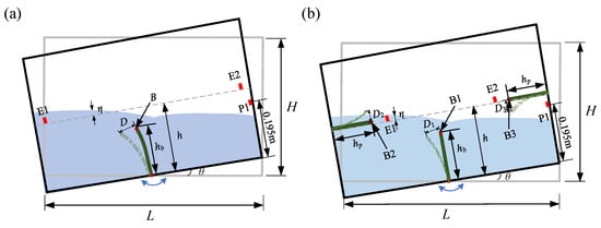
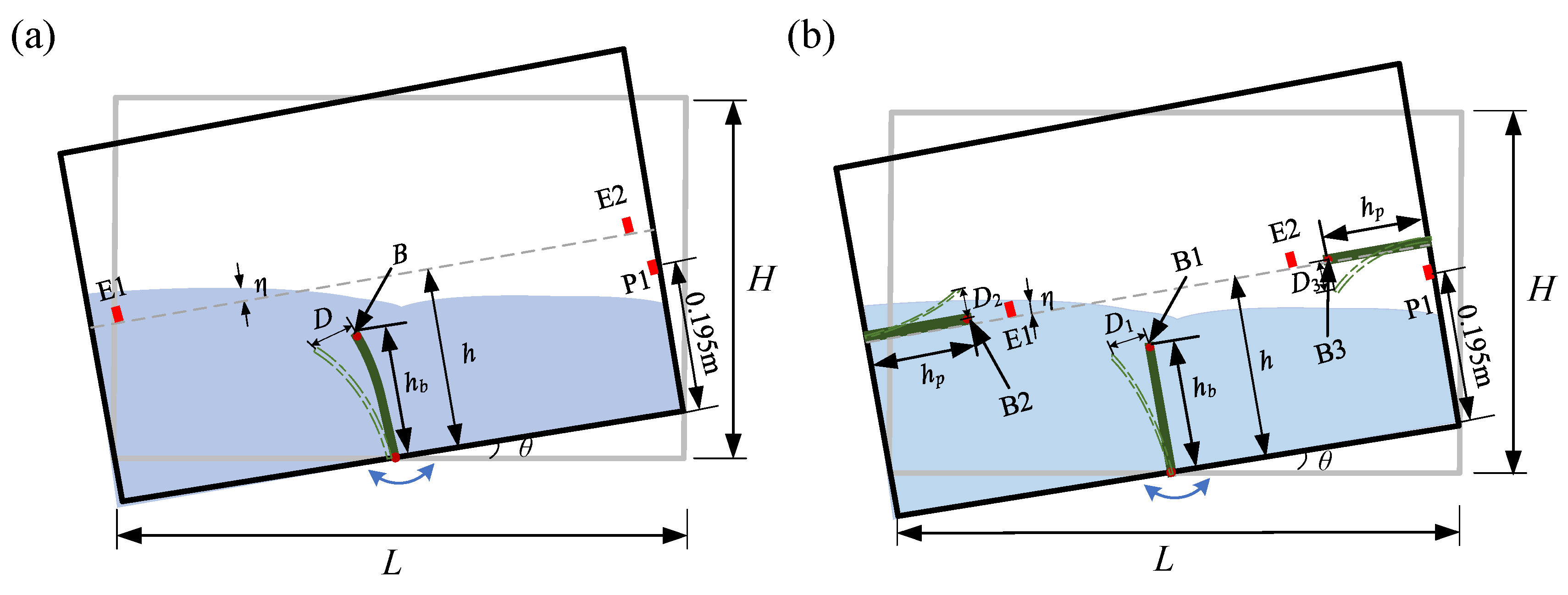
We considered a two-dimensional numerical setup for simulating the interaction between the sloshing and elastic baffles in a shaking tank, and the sketch for that is illustrated in Figure 1. To enhance the comprehension of the various symbols presented in the figure and the next context, we systematically summarized and clearly defined these symbols used and listed their values and units, as detailed in Table 1. We stressed that the distances between E1, E2, and the side walls are both 0.132 m, and the distance between P1 and the bottom wall is 0.195 m. Additionally, the motion equation of the shaking tank is

$$S\left(t\right)=\theta \mathrm{s}\mathrm{i}\mathrm{n} \omega t,$$

(25)

where $\theta$ is the shaking angle; $\omega$ is external excitation frequency.

Figure 1. A sketch for the problem of the interaction between sloshing water flow and elastic baffles in a shaking tank: (a) single elastic baffle; (b) multiple elastic baffles.

Table 1. Symbol definitions in the text.

Symbols	Definitions	Values	Units
$L$	width of the shaking tank	1.0	m
$H$	height of the shaking tank	0.72	m
${\rho }_W$	density of the sloshing water flow	1000.0	kg/m3
$\delta$	thickness of the elastic baffle	0.006	m
${\rho }_B$	density of the elastic baffle	1250.0	kg/m3
$\nu$	Poisson’s ratio of the elastic baffle	0.47	/
$E$	Young’s modulus of the elastic baffle	3.0 × 107	Pa
E1, E2	free surface elevation probes of the sloshing water flow	/	/
${\eta }_1$, ${\eta }_2$	free surface elevations of the sloshing water flow	/	m
B	displacement probe of the single elastic baffle’s top position	/	/
$D$	displacement of the single elastic baffle’s top position	/	m
$F$	force of the single elastic baffle’s top position	/	N
B1, B2, B3	displacement probes of the multiple elastic baffles’ top positions	/	/
$D_1$, $D_2$, $D_3$	displacements of the multiple elastic baffles’ top positions	/	m
$F_1$, $F_2$, $F_3$	forces of the multiple elastic baffles’ top positions	/	N
P1	pressure probe	/	/
$P$	impact pressure on the side wall of the shaking tank	/	KPa
$h$	filling water height of the shaking tank	0.244	m
$h_b$	height of the vertical elastic baffle	/	m
$h_p$	length of the horizontal elastic baffle	/	m
$\theta$	shaking angle of the tank	4~7	°
$\omega$	external excitation frequency	3.342~6.684	rad/s
${\omega }_1$	first-order resonant frequency of the tank	4.456	rad/s
$h/h_b$	immersion ratio	0.75~1.25	/

Moreover, to investigate the intrinsic correlation between the resonant frequency of the shaking tank and the motion response of the sloshing and elastic baffles, we calculated the resonant frequency of the water tank. Specifically, for a rectangular shaking tank with a given width and water filling depth, the linear analytical solution of the resonant frequency ${\omega }_n$ ($n=1,2,3\dots$) of the shaking tank can be solved by the theoretical equation proposed by Faltinsen et al. [28]:

$${\omega }_n=\sqrt{g{k}_n\mathrm{t}\mathrm{a}\mathrm{n}h\left(k_{n}h\right)}, (n=1, 2, 3\dots ).$$

(26)

where $k_n={\displaystyle \frac{2n-1}{L}}\pi$, ($n=1,2,3\dots$); $h$ is the filling water height; $g$ is the gravity acceleration; and $L$ is the width of the shaking tank. Therefore, we can obtain the first-order resonant frequency ${\omega }_1$ of the shaking tank without any elastic baffles under $h=0.244 \mathrm{m}$, whose value is 4.456 rad/s.

3.2. Convergence and Validation Study

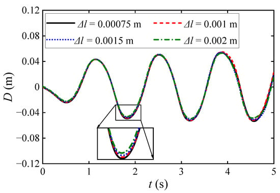
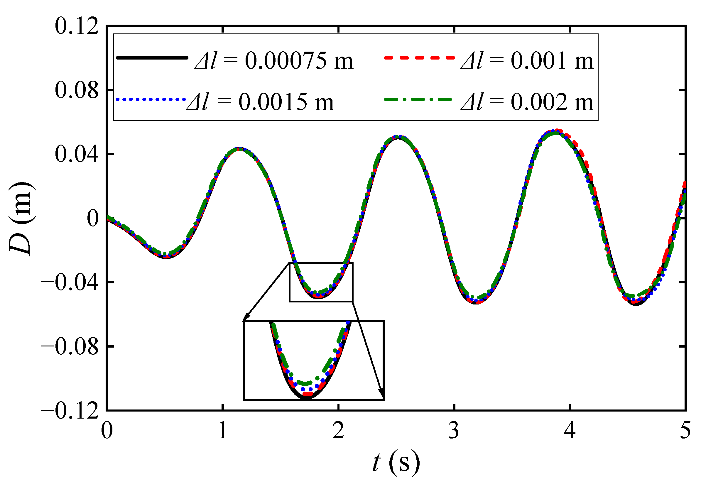
We conducted a convergence study for different initial particle spacings $∆l$, i.e., $∆l=0.00075 \mathrm{m}$, $0.001 \mathrm{m}$, $0.0015 \mathrm{m}$, and $0.002 \mathrm{m}$. Specifically, we plotted the various curves of $D$ versus $t$ under a single elastic baffle condition with $\omega =4.456 \mathrm{r}\mathrm{a}\mathrm{d}/\mathrm{s}$ and $h/h_b=1.25$, as illustrated in Figure 2. We stressed that the sizes of the fluid and solid particles are consistent. We can observe that as $∆l$ decreases, the curves of $D$ versus $t$ tend to coincide. Specifically, there is a specific gap between the curves with $∆l=0.0015 \mathrm{m}$ and $∆l=0.001 \mathrm{m}$, while the curves with $∆l=0.001 \mathrm{m}$ and $∆l=0.00075 \mathrm{m}$ almost overlap. To rigorously quantify this convergence beyond visual inspection, we calculated the Relative $L_2$ Error Norm between the displacement time-series of the chosen spacing ($∆l=0.001 \mathrm{m}$) and the finest spacing ($∆l=0.00075 \mathrm{m}$). The quantitative error measure was found to be exceptionally small at 4.04%, demonstrating strict numerical convergence. Additionally, the relative errors for coarser spacings of $∆l=0.0015 \mathrm{m}$ and $∆l=0.002 \mathrm{m}$ are 5.11% and 7.11%, respectively. Therefore, considering the need to balance computational accuracy and efficiency, we set $∆l=0.001 \mathrm{m}$ in all subsequent numerical simulations.

Figure 2. Convergence study for different initial particle spacings $∆l$. The inset shows a zoomed-in view of the various curves of $D$ versus $t$.

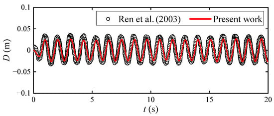
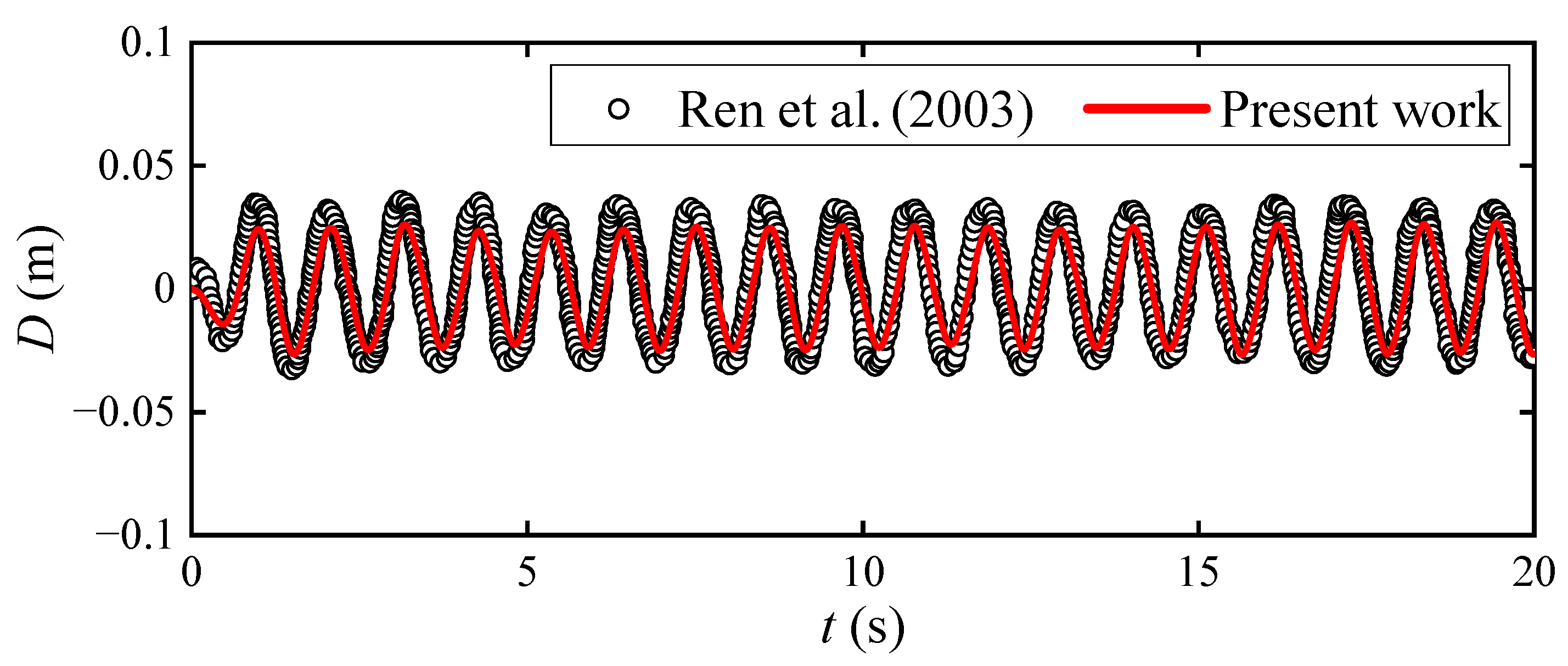
Moreover, we conducted a validation study comparing the present numerical work with the experiments of Ren et al. [18]. Specifically, we plotted the various curves of $D$ versus t under a single elastic baffle condition with identical parameters, as illustrated in Figure 3. We can observe that the numerical results are in good agreement with the experimental data. Thus, the proposed numerical model is applicable for simulating the interaction between the sloshing and single or multiple elastic baffles in a shaking tank.

Figure 3. Validation between the present numerical work and the experiment data of Ren et al. [18].

It should be noted that while the present validation demonstrates the accuracy of the numerical model in capturing the structural displacement of a single elastic baffle, validation for wall impact pressure and multiple-baffle configurations is not explicitly presented. This limitation stems from the current scarcity of comprehensive experimental data in the open literature that simultaneously measures localized dynamic pressures and multi-baffle hydro-elastic responses under shaking excitation. Nevertheless, because the multiple-baffle conditions and pressure calculations rely on the identical, fundamentally validated SPH-FSI governing equations and coupling algorithms as the single-baffle case, the numerical model is considered robust, self-consistent, and theoretically reliable for extending the investigation to these complex scenarios.

4. Results and Discussion

4.1. Single Elastic Baffle

We specifically investigate the free surface elevations of the sloshing ${\eta }_1$ and ${\eta }_2$, the displacement and force of the single elastic baffle’s top position $D$ and $F$, the impact pressure on the side wall $P$ under different external incentive frequencies $\omega$, shnking angles $\theta$, and immersion ratios $h/h_b$ to illustrate the mechanism of interaction between the sloshing and the single elastic baffle in a shaking tank.

4.1.1. Influence of $\mathit{\omega }$

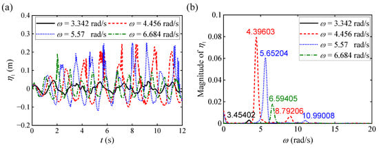
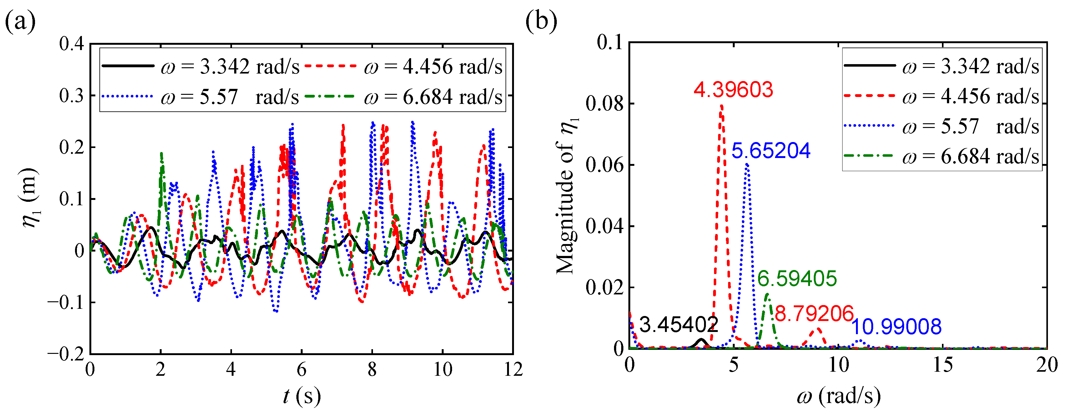
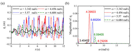
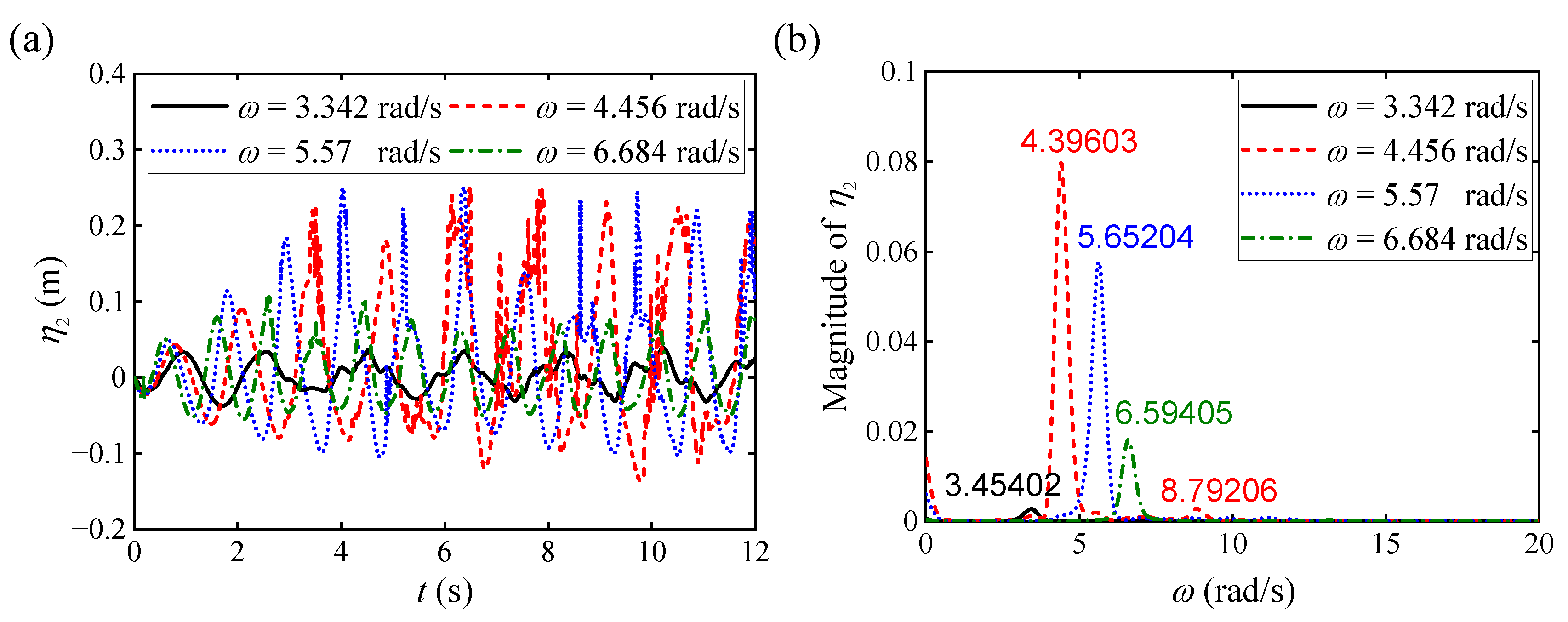
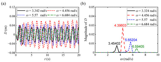
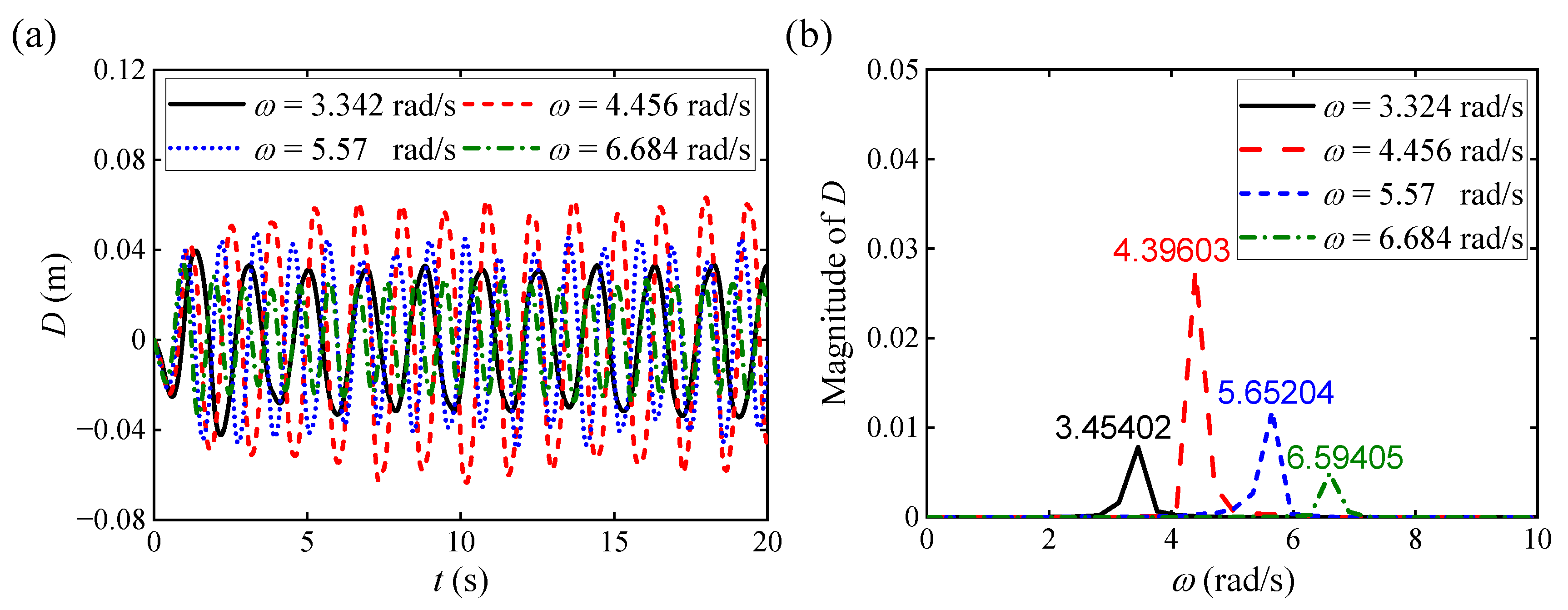
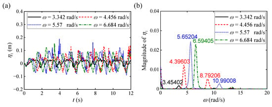
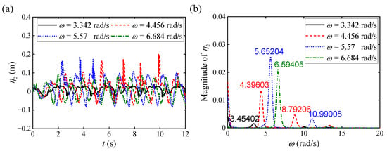
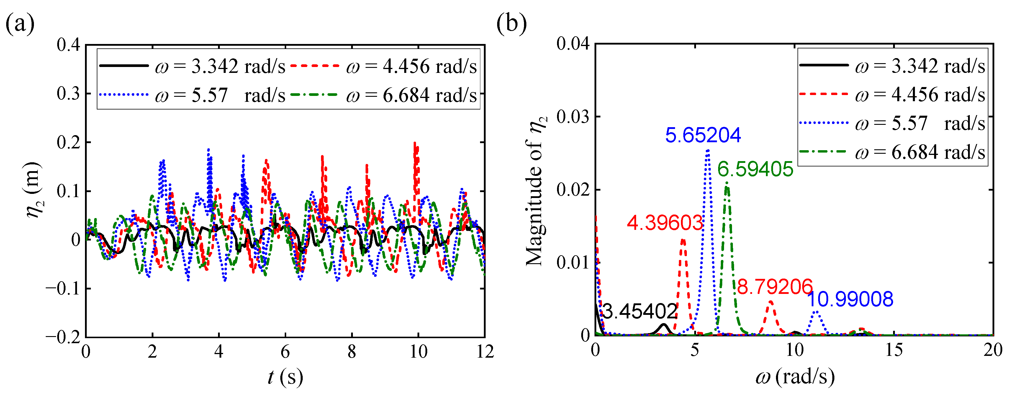
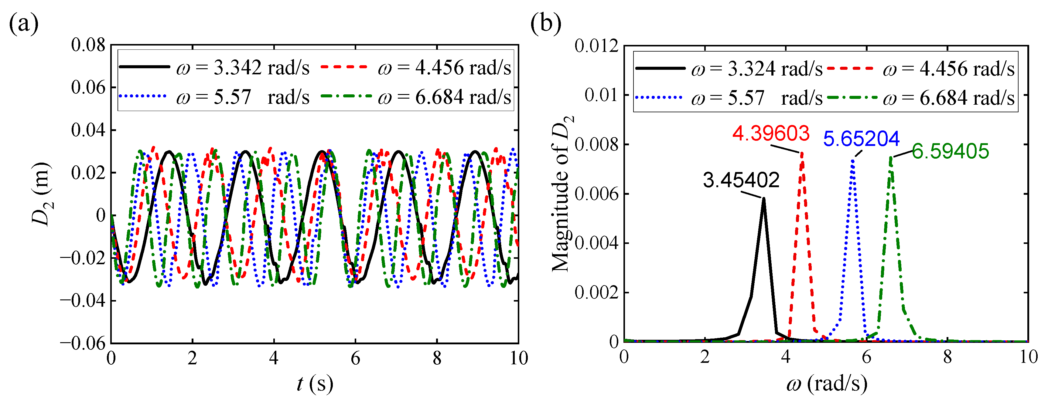
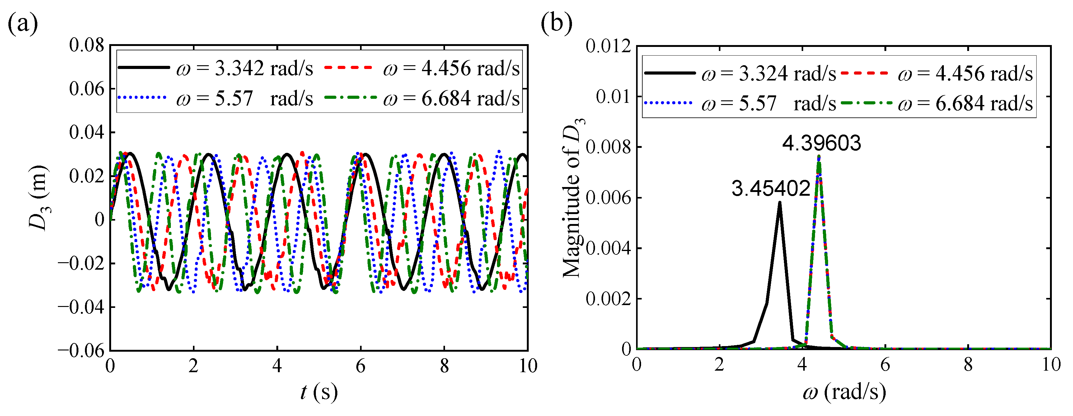
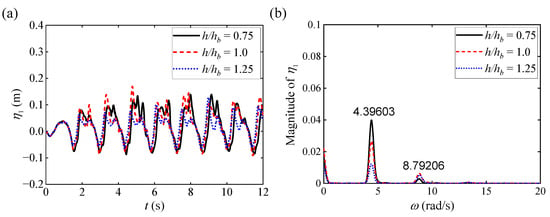
We specifically conduct numerical simulations under $\omega =3.342$, $4.456$, $5.57$, and $6.684$ $\mathrm{r}\mathrm{a}\mathrm{d}/\mathrm{s}$, while keeping $\theta =4^{\mathrm{o}}$ and $h/h_b=1.25$ constant to investigate the influence of $\omega$ on the interaction between the sloshing and the single elastic baffle. We first plot the various curves of ${\eta }_1$ and ${\eta }_2$ versus $t$ under different $\omega$with a single elastic baffle, as illustrated in Figure 4a and Figure 5a, respectively. It can be observed from the above two figures that the free surface elevation fluctuation period of the sloshing exhibits a significant frequency dependence on $\omega$. Specifically, the amplitude of ${\eta }_1$ and ${\eta }_2$ under $\omega =4.456$ and $5.57$ $\mathrm{r}\mathrm{a}\mathrm{d}/\mathrm{s}$ is more significant than that under $\omega =3.342$ and $6.684$ $\mathrm{r}\mathrm{a}\mathrm{d}/\mathrm{s}$, exhibiting more severe sloshing response characteristics. Given that it is difficult to accurately compare time-domain waveforms in Figure 4a and Figure 5a, we utilize the Fast Fourier Transformation (FFT) analysis method to obtain the magnitude of ${\eta }_1$ and ${\eta }_2$ under different $\omega$ with a single elastic baffle, as illustrated in Figure 4b and Figure 5b, respectively. It can be observed from the above two figures that the FFT spectral response analysis not only verifies the consistency of time-domain observation results, but also reveals that the magnitude at $\omega =4.456$ $\mathrm{r}\mathrm{a}\mathrm{d}/\mathrm{s}$ is higher than that at $\omega =5.57$ $\mathrm{r}\mathrm{a}\mathrm{d}/\mathrm{s}$. Additionally, under $\omega =3.342$ and $6.684$ $\mathrm{r}\mathrm{a}\mathrm{d}/\mathrm{s}$, the energy of the sloshing is mainly concentrated in the resonant frequency (${\omega }_1=4.456 \mathrm{r}\mathrm{a}\mathrm{d}/\mathrm{s}$); under $\omega =4.456$ and $5.57$ $\mathrm{r}\mathrm{a}\mathrm{d}/\mathrm{s}$, the spectrum exhibits a noticeable distribution of second harmonic energy at $8.79206$ and $10.99008$ rad/s. This spectral feature suggests a potential association with nonlinear wave interactions, although further targeted investigations would be required to fully establish this underlying mechanism when the second harmonic waves occur [29]. In summary, under the excitation of intermediate frequencies (namely $\omega =4.456$ and $5.57$ $\mathrm{r}\mathrm{a}\mathrm{d}/\mathrm{s}$), the plotted trends suggest that the sloshing water flow likely undergoes more complex energy conversion processes, exhibiting behaviors characteristic of nonlinear dynamics. The combined effect of the resonant frequency and harmonic movement of the shaking tank leads to intensified water flow. When $\omega$ approaches ${\omega }_1$, the shaking tank exhibits typical resonance response characteristics.

Figure 4. Numerical results for ${\eta }_1$ under different $\omega$ with a single elastic baffle: (a) various curves of ${\eta }_1$ versus $t$; (b) corresponding FFT analysis of ${\eta }_1$.

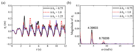
Figure 5. Numerical results for ${\eta }_2$ under different $\omega$ with a single elastic baffle: (a) various curves of ${\eta }_2$ versus $t$; (b) corresponding FFT analysis of ${\eta }_2$.

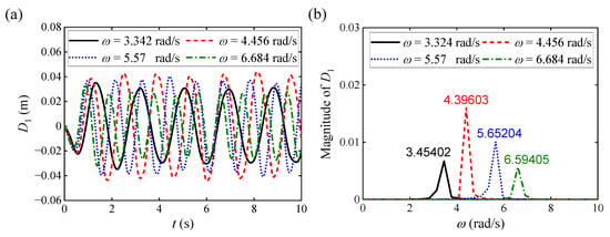
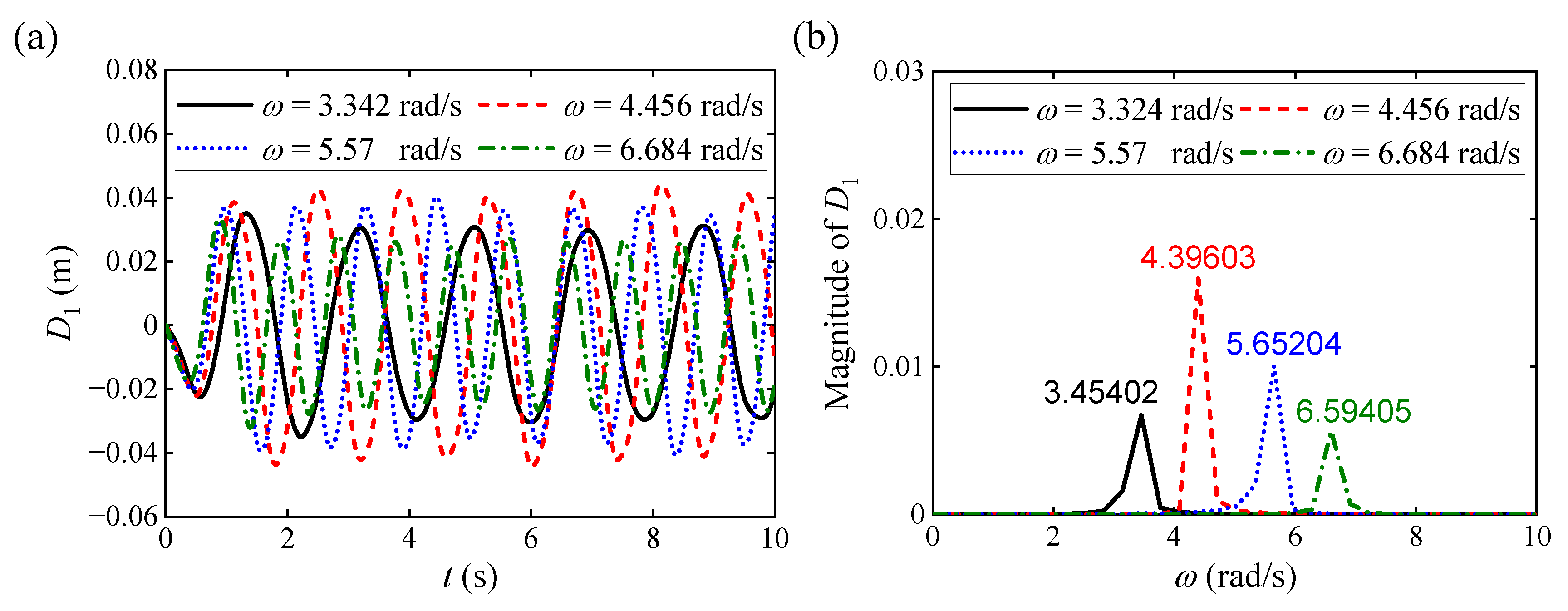
We next plot the various curves of $D$ versus $t$ and the corresponding FFT analysis results of $D$ under different $\omega$ with a single elastic baffle, as illustrated in Figure 6a and Figure 6b, respectively. The results demonstrate that the amplitude of $D$ under $\omega =4.456$ and $5.57$ $\mathrm{r}\mathrm{a}\mathrm{d}/\mathrm{s}$ is more significant than that under $\omega =3.342$ and $6.684$ $\mathrm{r}\mathrm{a}\mathrm{d}/\mathrm{s}$, exhibiting more severe sloshing response characteristics; when $\omega$ approaches ${\omega }_1$, the bending deformation amplitude of the elastic baffle reaches its maximum. For instance, the maximum displacement $D$ at the resonant frequency (${\omega }_1=4.456$ $\mathrm{r}\mathrm{a}\mathrm{d}/\mathrm{s}$) is approximately $0.06 \mathrm{m}$, which represents a substantial amplification of 2.0 times compared to the off-resonance condition at $\omega =3.342$ $\mathrm{r}\mathrm{a}\mathrm{d}/\mathrm{s}$ (where the peak $D$ is only approximately $0.03 \mathrm{m}$). Combining the previous analysis conclusions, we can conclude that $D$ exhibits strong consistency with ${\eta }_1$ and ${\eta }_2$, indicating a close dynamic relationship between them under FSI. Additionally, the FFT analysis results in Figure 6b further confirm this trend, with the baffle reaching its maximum bending response amplitude at $\omega =4.456 \mathrm{r}\mathrm{a}\mathrm{d}/\mathrm{s}$.

Figure 6. Numerical results for $D$ under different $\omega$ with a single elastic baffle: (a) various curves of $D$ versus $t$; (b) corresponding FFT analysis of $D$.

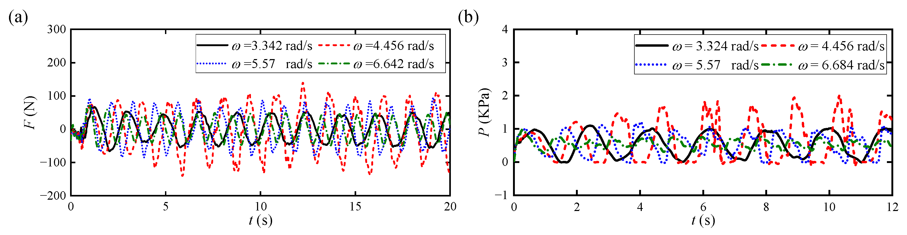
We finally plot the various curves of $F$ and $P$ versus $t$ under different $\omega$ with a single elastic baffle, as illustrated in Figure 7a and Figure 7b, respectively. The results demonstrate that the trend of $F$versus $t$ is similar to that of $D$, which further verifies the significant influence of FSI on the dynamic response of the elastic baffle. Furthermore, we can conclude that $P$ does not increase linearly with $\omega$. In contrast, when $\omega$ approaches ${\omega }_1$, $P$ reaches its maximum value. Quantitatively, the peak impact pressure surges to 2.0 kPa at $\omega =4.456 \mathrm{r}\mathrm{a}\mathrm{d}/\mathrm{s}$, exhibiting an increase of 150% relative to the non-resonant high-frequency excitation ($\omega =$ $6.684 \mathrm{r}\mathrm{a}\mathrm{d}/\mathrm{s}$). This result indicates that the matching between $\omega$ and ${\omega }_1$ is a key factor in triggering resonance and causing pressure peaks.

Figure 7. Various curves of $F$ and $P$ versus $t$ under different $\omega$ with a single elastic baffle: (a) $F$; (b) $P$.

To further elucidate the underlying mechanism of these observations, we clarify why the elastic baffle exhibits fundamentally distinct fluid–structure interaction behavior compared to a conventional rigid baffle. Whereas rigid baffles suppress sloshing predominantly via physical flow obstruction and enforced wave reflection, the elastic baffle enables a coupled hydro-elastic damping mechanism rooted in energy exchange and dynamic phase modulation. First, from an energy perspective, the baffle’s bending deformation absorbs a portion of the fluid’s kinetic energy and converts it into recoverable structural strain energy, thereby introducing a supplementary, intrinsic dissipation pathway beyond viscous or turbulent losses. Second, the baffle’s dynamic restoring force induces a consistent phase lag between the incident sloshing wave motion and its structural response; this phase shift actively desynchronizes the fluid’s resonant buildup, directly accounting for the broadened spectral distribution and elevated harmonic conversion efficiency observed in the FFT analysis. Third, the time-varying deformation continuously reshapes the tank’s effective internal geometry, thereby modulating the instantaneous resonant frequency of the local fluid domain; this transient frequency detuning impedes sustained resonance locking at any fixed modal frequency, enhancing broadband suppression performance.

4.1.2. Influence of $\mathit{\theta }$

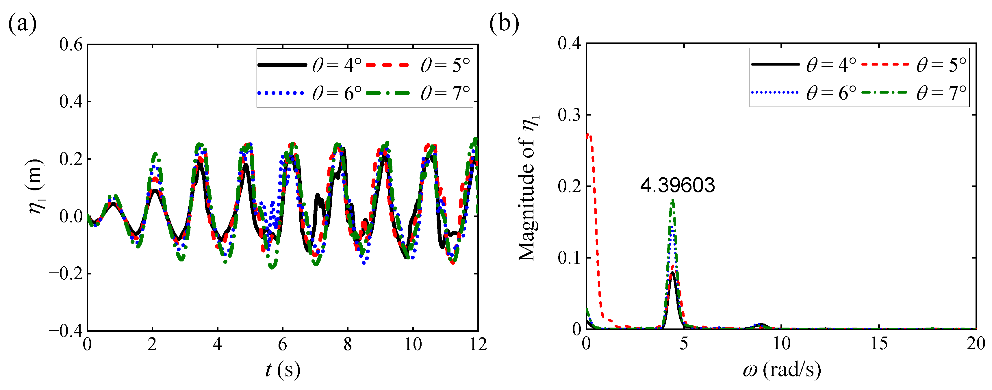
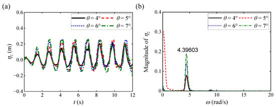
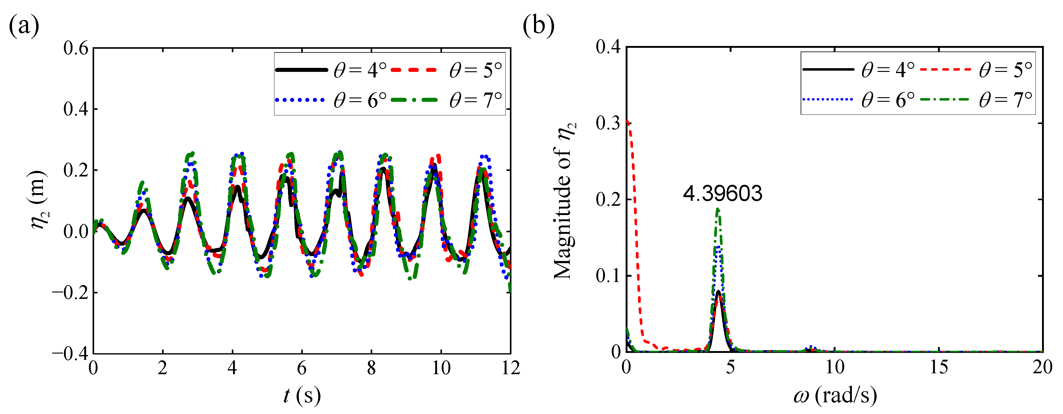
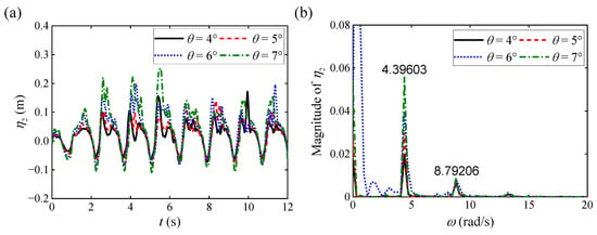
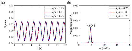
We specifically conduct numerical simulations under $\theta =4^{\mathrm{o}}$, $5^{\mathrm{o}}$, $6^{\mathrm{o}}$, and $7^{\mathrm{o}}$, while keeping $\omega =4.456$ $\mathrm{r}\mathrm{a}\mathrm{d}/\mathrm{s}$ and $h/h_b=1.25$ constant to investigate the influence of $\theta$ on the interaction between sloshing and the single elastic baffle. We first plot the various curves of ${\eta }_1$ and ${\eta }_2$ versus $t$ under different $\theta$ with a single elastic baffle, as illustrated in Figure 8a and Figure 9a, respectively. It can be observed from the above two figures that under different $\theta$ with a single elastic baffle, the overall evolution characteristics of the sloshing remain consistent; as $\theta$ increases, the amplitudes of ${\eta }_1$ and ${\eta }_2$ show a significant increasing trend. This phenomenon indicates that the dynamic behavior of the sloshing is greatly affected by the nonlinear effects of $\theta$. Furthermore, we plot the magnitude of ${\eta }_1$ and ${\eta }_2$ under different $\theta$ with a single elastic baffle using FFT analysis, as illustrated in Figure 8b and Figure 9b, respectively. It can be observed from the above two figures that when $\theta =7^{\mathrm{o}}$, the response amplitudes of ${\eta }_1$ and ${\eta }_2$ reach their maximum.

Figure 8. Numerical results for ${\eta }_1$ under different $\theta$ with a single elastic baffle: (a) various curves of ${\eta }_1$ versus $t$; (b) corresponding FFT analysis of ${\eta }_1$.

Figure 9. Numerical results for ${\eta }_2$ under different $\theta$ with a single elastic baffle: (a) various curves of ${\eta }_1$ versus $t$; (b) corresponding FFT analysis of ${\eta }_2$.

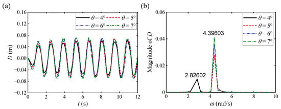
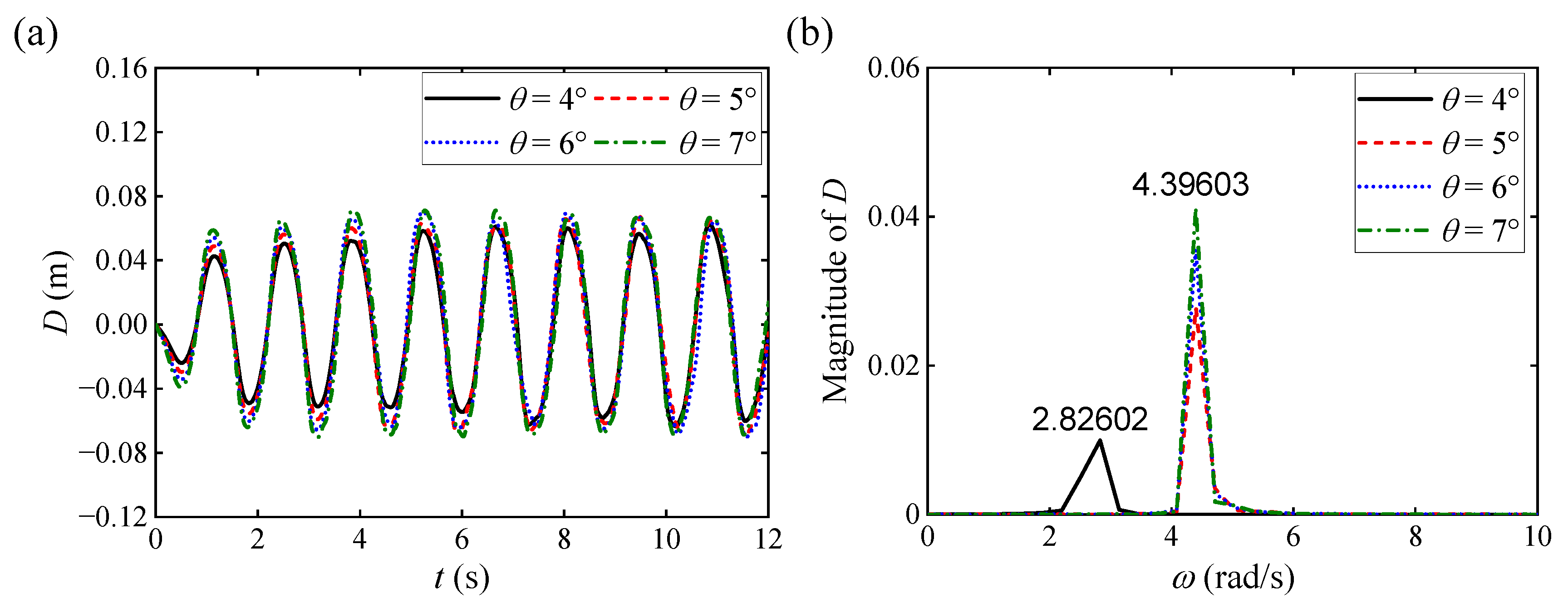
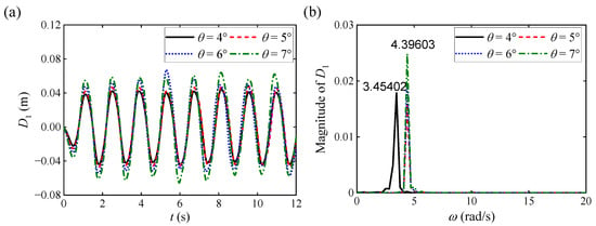
We next plot the various curves of $D$ versus $t$ and the corresponding FFT analysis results of $D$ under different $\theta$ with a single elastic baffle, as illustrated in Figure 10a and Figure 10b, respectively. The results demonstrate that $D$ shows a high degree of consistency with the dynamic variation characteristics of ${\eta }_1$ and ${\eta }_2$, especially at $\omega =4.456$ $\mathrm{r}\mathrm{a}\mathrm{d}/\mathrm{s}$, where they both exhibit significant resonance phenomena. FFT analysis in Figure 10b further verifies this result, and specifically, the magnitude of $D$ under various $\theta$ reached its maximum value around $\omega =4.456$ $\mathrm{r}\mathrm{a}\mathrm{d}/\mathrm{s}$. Additionally, as $\theta$ increases, the magnitude of $D$ exhibits a significant increasing trend, which is consistent with the trends of ${\eta }_1$ and ${\eta }_2$in Figure 8b and Figure 9b.

Figure 10. Numerical results for $D$ under different $\theta$ with a single elastic baffle: (a) various curves of $D$ versus $t$; (b) corresponding FFT analysis of $D$.

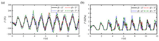
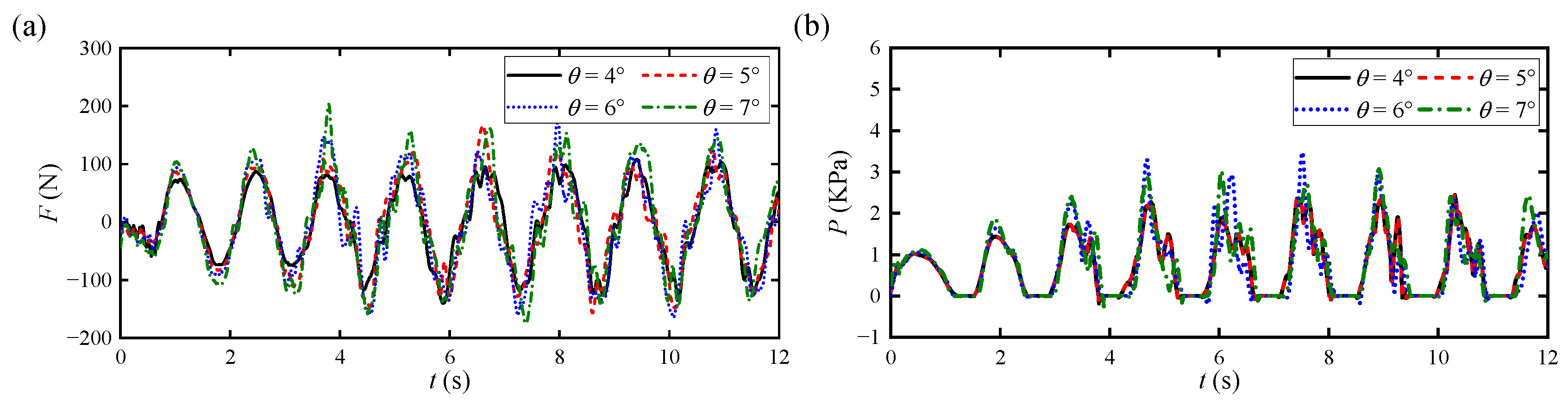
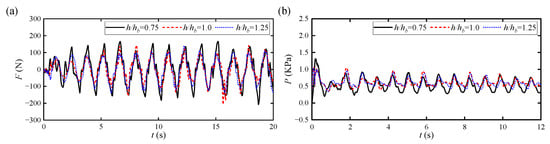
We finally plot the various curves of $F$ and $P$ versus $t$ under different $\theta$ with a single elastic baffle, as illustrated in Figure 11a and Figure 11b, respectively. The results demonstrate that the trend of $F$versus $t$ is similar to that of $D$, which further verifies the significant influence of FSI on the dynamic response of the elastic baffle. When $\omega$ approaches ${\omega }_1$, the amplitude of $F$ acting on the baffle reaches its maximum value, indicating that the elastic baffle is subjected to strong fluid forces at the resonant frequency. Additionally, as $\theta$ increases, the amplitude of $P$ increases notably, suggesting more intense sloshing behavior of the water flow.

Figure 11. Various curves of $F$ and $P$ versus $t$ under different $\theta$ with a single elastic baffle: (a) $F$; (b) $P$.

4.1.3. Influence of $\mathit{h}/{\mathit{h}}_{\mathit{b}}$

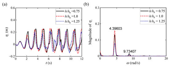
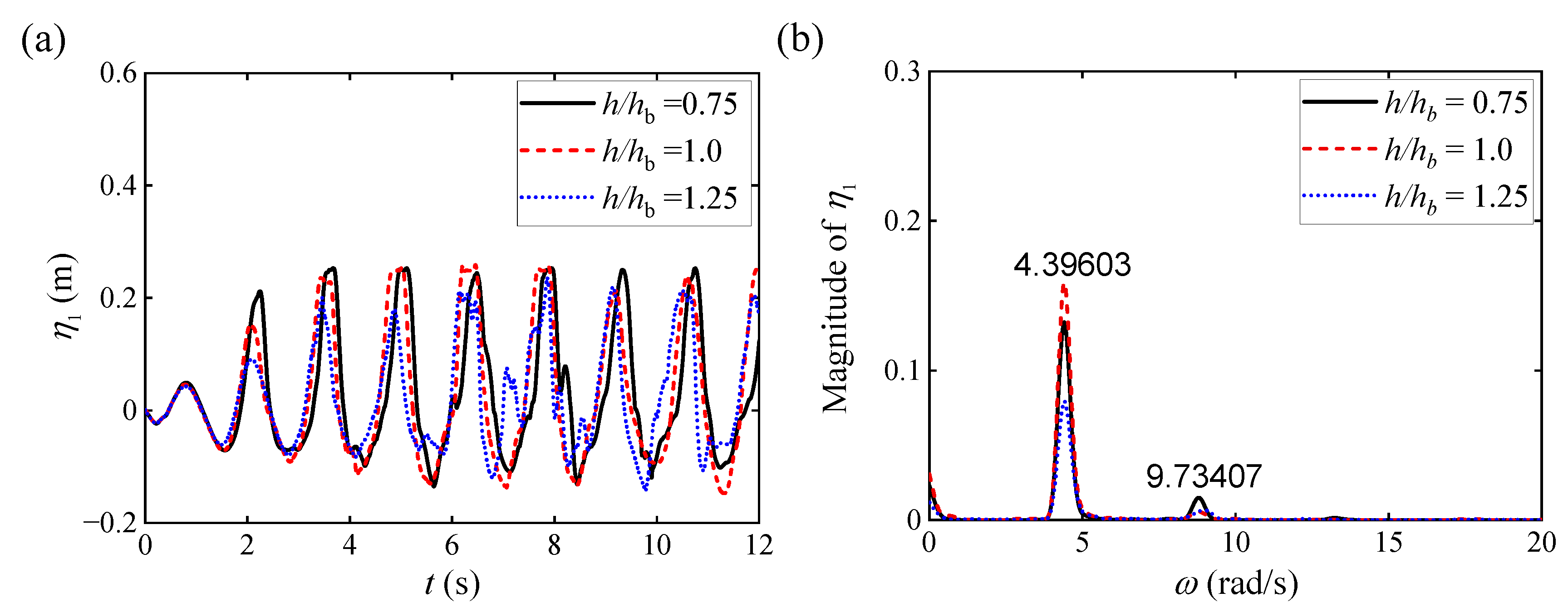
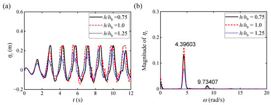
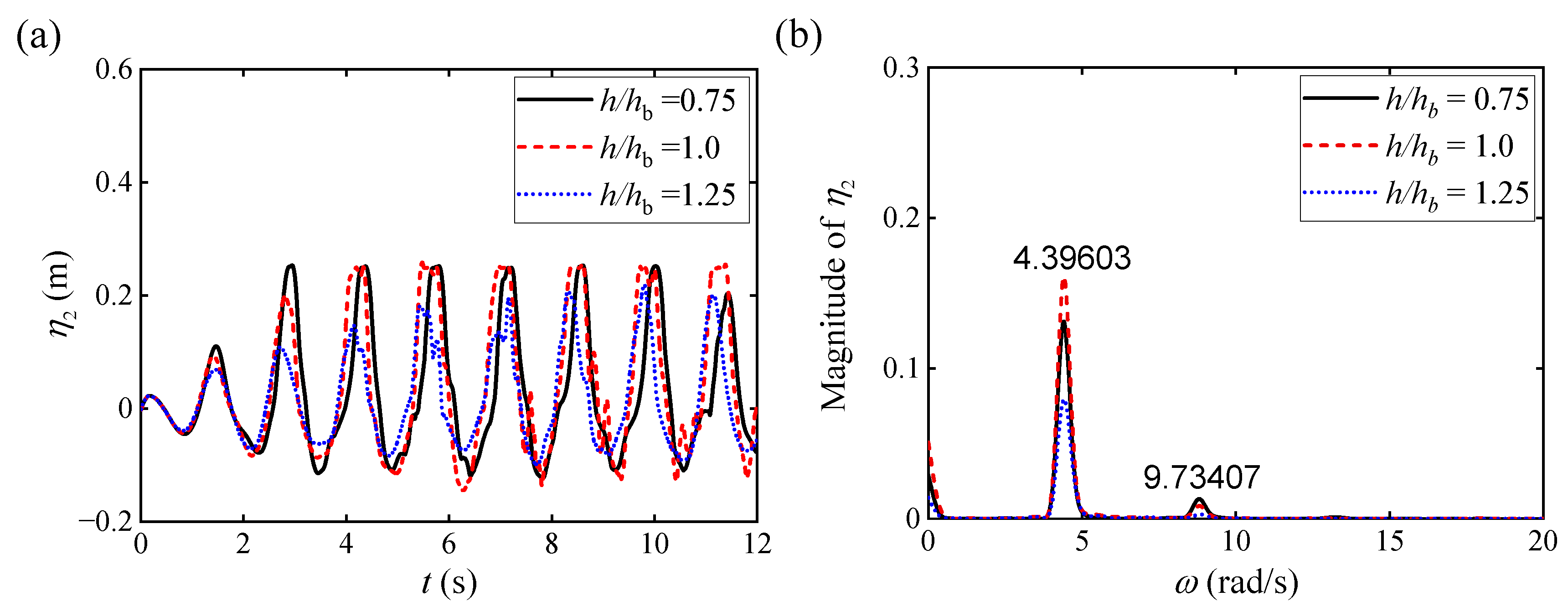
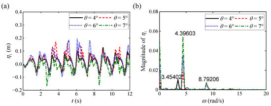
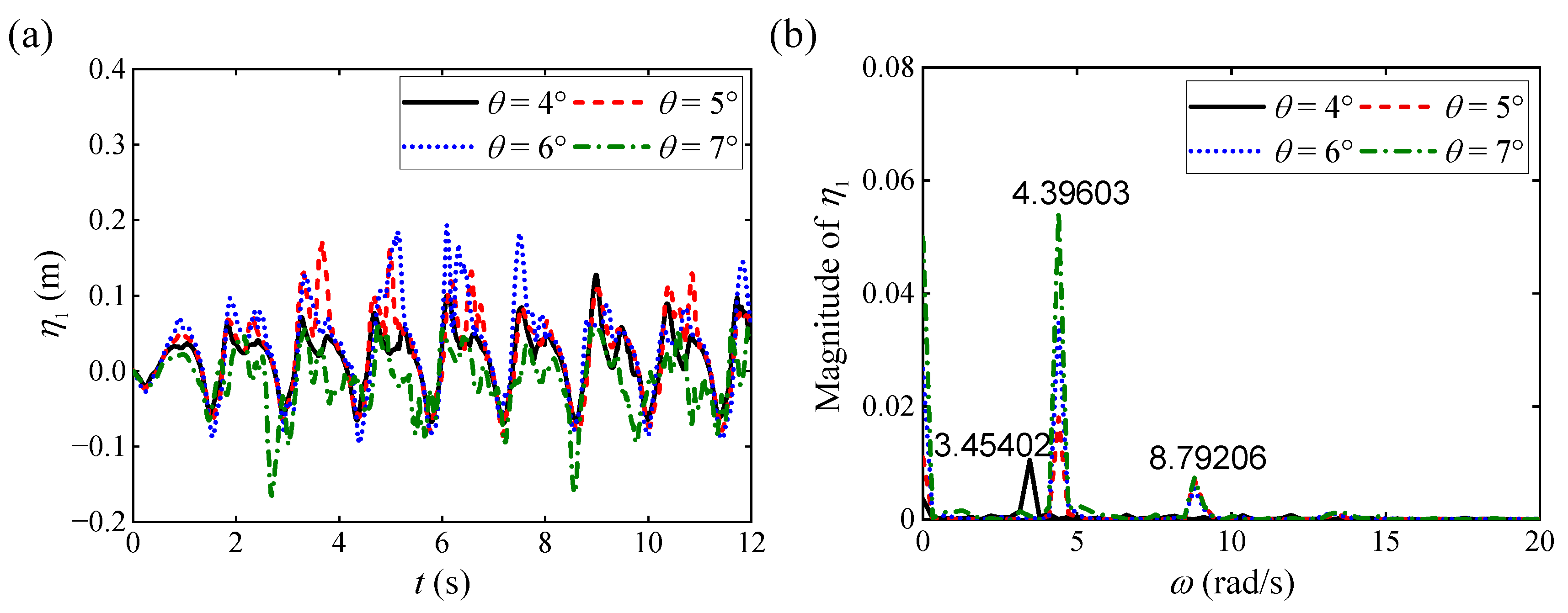
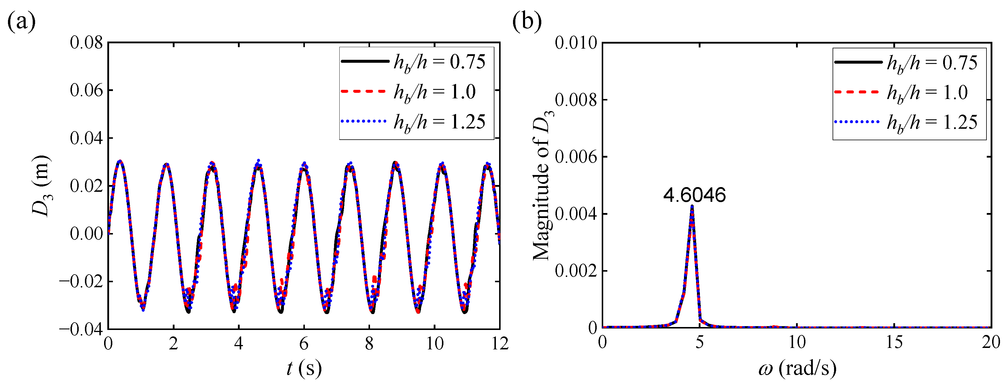
We specifically conduct numerical simulations under $h/h_b=0.75$, $1.0$, and $1.25$, while keeping $\omega =4.456$ $\mathrm{r}\mathrm{a}\mathrm{d}/\mathrm{s}$ and $\theta =4^{\mathrm{o}}$ constant to investigate the influence of $h/h_b$ on the interaction between the sloshing and the single elastic baffle. We first plot the various curves of ${\eta }_1$ and ${\eta }_2$ versus $t$ under different $h/h_b$ with a single elastic baffle, as illustrated in Figure 12a and Figure 13a, respectively. It can be observed from the above two figures that under different $h/h_b$ with a single elastic baffle, the amplitudes of ${\eta }_1$ and ${\eta }_2$ are relatively close when $h/h_b=0.75$ and $1.0$ and gradually decrease when $h/h_b=1.25$. Furthermore, we plot the magnitude of ${\eta }_1$ and ${\eta }_2$ under different $h/h_b$ with a single elastic baffle using FFT analysis, as illustrated in Figure 12b and Figure 13b, respectively. It can be observed from the above two figures that the motion response of the sloshing occurs at $\omega =4.39603$ and $9.73407$ $\mathrm{r}\mathrm{a}\mathrm{d}/\mathrm{s}$, which are close to ${\omega }_1$ and twice ${\omega }_1$. Additionally, when $\omega =4.39603 \mathrm{r}\mathrm{a}\mathrm{d}/\mathrm{s}$, the maximum amplitudes of ${\eta }_1$ and ${\eta }_2$ occur at $h/h_b=1.0$; while $\omega =9.73407 \mathrm{r}\mathrm{a}\mathrm{d}/\mathrm{s}$, the maximum amplitudes of ${\eta }_1$ and ${\eta }_2$ occur at $h/h_b=0.75$ and gradually decrease with the increase in $h/h_b$.

Figure 12. Numerical results for ${\eta }_1$ under different $h/h_b$ with a single elastic baffle: (a) various curves of ${\eta }_1$ versus $t$; (b) corresponding FFT analysis of ${\eta }_1$.

Figure 13. Numerical results for ${\eta }_2$ under different $h/h_b$ with a single elastic baffle: (a) various curves of ${\eta }_2$ versus $t$; (b) corresponding FFT analysis of ${\eta }_2$.

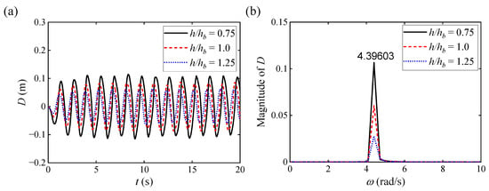
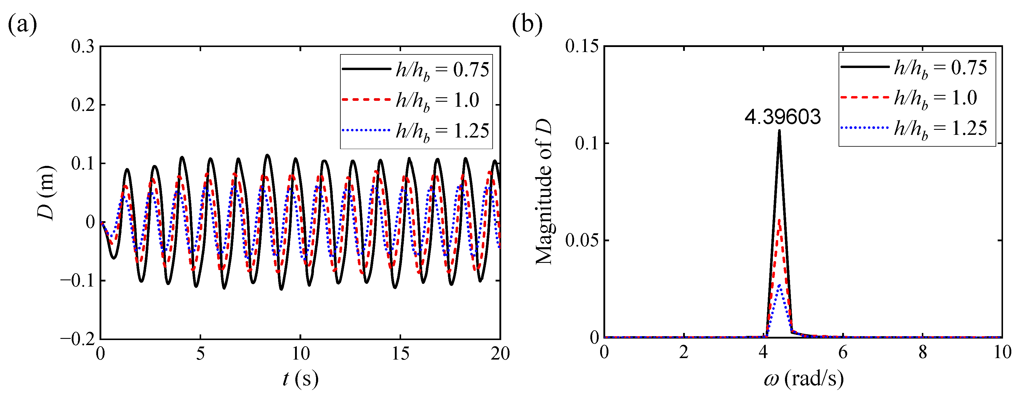
We next plot the various curves of $D$ versus $t$ and the corresponding FFT analysis results of $D$ under different $h/h_b$ with a single elastic baffle, as illustrated in Figure 14a and Figure 14b, respectively. The results demonstrate that as $h/h_b$ increases, $D$ gradually decreases, exhibiting a negative correlation with $h/h_b$. FFT analysis in Figure 14b further verifies that as $h/h_b$ increases, $D$ shows a gradually decreasing trend. Additionally, the magnitude of $D$ under various $h/h_b$ reached its maximum value at $\omega =4.39603$ $\mathrm{r}\mathrm{a}\mathrm{d}/\mathrm{s}$.

Figure 14. Numerical results for $D$ under different $h/h_b$ with a single elastic baffle: (a) various curves of $D$ versus $t$; (b) corresponding FFT analysis of $D$.

We finally plot the various curves of $F$ and $P$ versus $t$ under different $h/h_b$ with a single elastic baffle, as illustrated in Figure 15a and Figure 15b, respectively. The results demonstrate that $F$ exhibits a characteristic change consistent with $D$. Specifically, under $h/h_b=0.75$ and $1.0$, $F$ exhibits obvious nonlinear characteristics, which may be related to the non-uniformity of hydrodynamic excitation and the complex deformation mode of the elastic baffle at lower $h/h_b$; as $h/h_b$ increases, this nonlinear characteristic gradually weakens. Additionally, as $h/h_b$ increases, the amplitude of $P$ decreases notably, which is consistent with the trend of $F$ versus $t$.

Figure 15. Various curves of $F$ and $P$ versus $t$ under different $h/h_b$ with a single elastic baffle: (a) $F$; (b) $P$.

4.2. Multiple Elastic Baffles

We specifically investigate the free surface elevations of the sloshing ${\eta }_1$ and ${\eta }_2$, the displacement and force of the multiple elastic baffles’ top position $D_1$, $D_2$, $D_3$ and $F_1$, $F_2$, $F_3$, the impact pressure on the side wall $P$ under different external incentive frequencies $\omega$, shaking angles $\theta$, and immersion ratios $h/h_b$ to illustrate the mechanism of interaction between the sloshing and the multiple elastic baffles in a shaking tank.

4.2.1. Influence of $\mathit{\omega }$

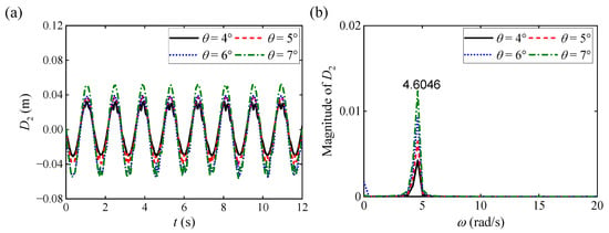
We specifically conduct numerical simulations under $\omega =3.342$, $4.456$, $5.57$, and $6.684$ $\mathrm{r}\mathrm{a}\mathrm{d}/\mathrm{s}$, while keeping $\theta =4^{\mathrm{o}}$ and $h/h_b=1.25$ constant to investigate the influence of $\omega$ on the interaction between the sloshing and the multiple elastic baffles. We first plot the various curves of ${\eta }_1$ and ${\eta }_2$ versus $t$ under different $\omega$ with multiple elastic baffles, as illustrated in Figure 16a and Figure 17a, respectively. It can be observed from the above two figures that, similar to Figure 4a and Figure 5a, the free surface elevation fluctuation period of the sloshing also exhibits a significant frequency dependence on $\omega$. Specifically, ${\eta }_1$ and ${\eta }_2$ under $\omega =5.57$ and $6.684$ $\mathrm{r}\mathrm{a}\mathrm{d}/\mathrm{s}$ is more significant than that under $\omega =3.342$ and $4.456$ $\mathrm{r}\mathrm{a}\mathrm{d}/\mathrm{s}$, exhibiting more severe sloshing response characteristics. We stress that, compared to the single elastic baffle condition, the multiple elastic baffles condition shifts the resonance frequency of the shaking tank to a higher value. Given that it is difficult to accurately compare time-domain waveforms in Figure 16a and Figure 17a, we utilize the FFT analysis method to obtain the magnitude of ${\eta }_1$ and ${\eta }_2$ under different $\omega$ with multiple elastic baffles, as illustrated in Figure 16b and Figure 17b, respectively. It can be observed from the above two figures that the FFT spectral response analysis not only verifies the consistency of time-domain observation results, but also reveals that the magnitude at $\omega =5.57$ and $6.684$ $\mathrm{r}\mathrm{a}\mathrm{d}/\mathrm{s}$ is higher than that at $\omega =3.342$ and $4.456$ $\mathrm{r}\mathrm{a}\mathrm{d}/\mathrm{s}$. Additionally, under $\omega =3.342$ and $6.684$ $\mathrm{r}\mathrm{a}\mathrm{d}/\mathrm{s}$, the energy of the sloshing is mainly concentrated in components higher than that at ${\omega }_1=4.456$ $\mathrm{r}\mathrm{a}\mathrm{d}/\mathrm{s}$; under $\omega =4.456$ and $5.57$ $\mathrm{r}\mathrm{a}\mathrm{d}/\mathrm{s}$, the spectrum shows a significant distribution of double harmonic energy (corresponding to $\omega =8.79206$ and $10.99008$ $\mathrm{r}\mathrm{a}\mathrm{d}/\mathrm{s}$), which is closely related to the interaction mechanism of nonlinear waves, which is verified by the occurrence of double harmonics. In summary, under the excitation of higher frequencies (namely, $\omega =5.57$ and $6.684$ $\mathrm{r}\mathrm{a}\mathrm{d}/\mathrm{s}$), the sloshing exhibits higher energy conversion efficiency and significant nonlinear characteristics. The combined effect of the higher frequency and harmonic movement of the shaking tank leads to intensified water flow.

Figure 16. Numerical results for ${\eta }_1$ under different $\omega$ with multiple elastic baffles: (a) various curves of ${\eta }_1$ versus $t$; (b) corresponding FFT analysis of ${\eta }_1$.

Figure 17. Numerical results for ${\eta }_2$ under different $\omega$ with multiple elastic baffles: (a) various curves of ${\eta }_2$ versus $t$; (b) corresponding FFT analysis of ${\eta }_2$.

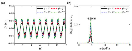
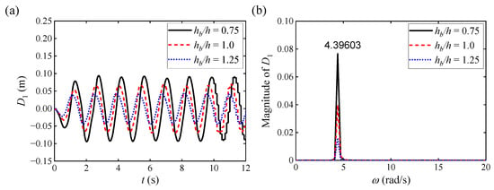
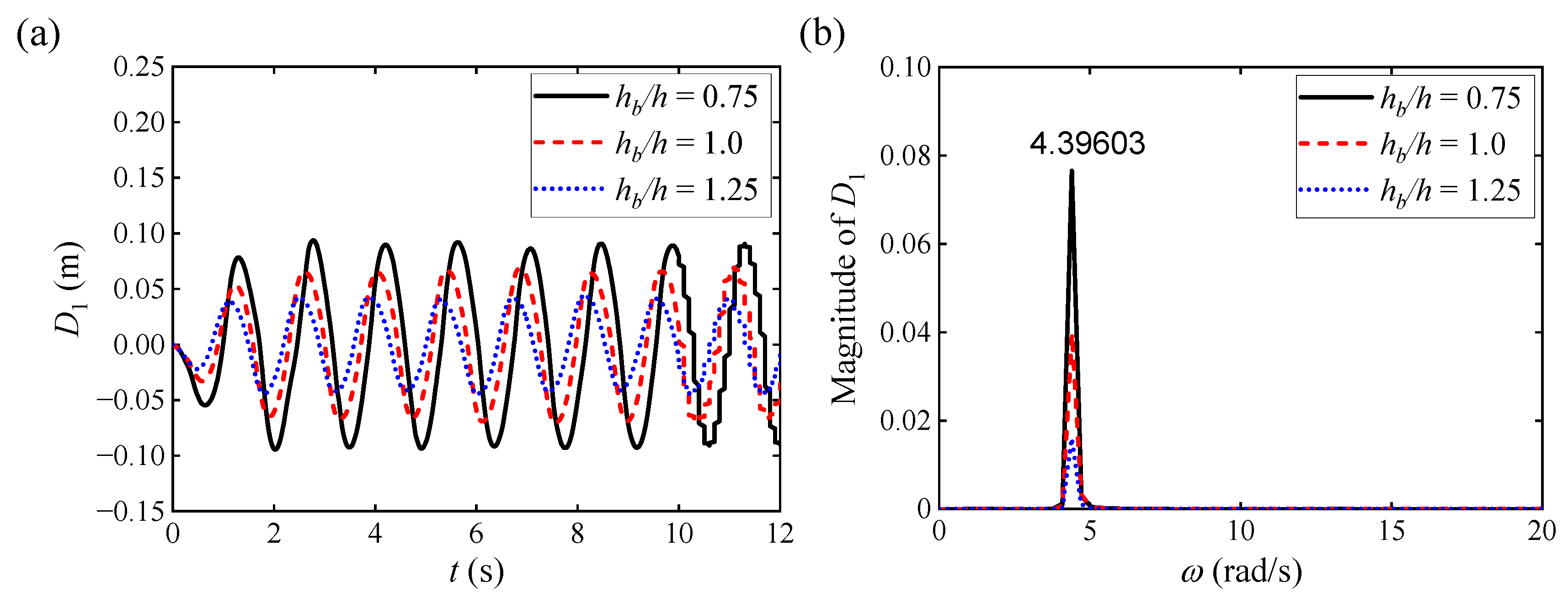
We next plot the various curves of $D_1$, $D_2$, $D_3$ versus $t$ and the corresponding FFT analysis results of $D_1$, $D_2$, $D_3$ under different $\omega$ with multiple elastic baffles, as illustrated in Figure 18a, Figure 19a, Figure 20a and Figure 18b, Figure 19b, Figure 20b, respectively. The results demonstrate that the amplitude of $D_1$ under approximately ${\omega }_1=4.456$ $\mathrm{r}\mathrm{a}\mathrm{d}/\mathrm{s}$ is more significant than that under other $\omega$, exhibiting more severe sloshing response characteristics; when $\omega$ approaches ${\omega }_1$, the bending deformation amplitude of the elastic baffle reaches its maximum. For instance, the maximum displacement ($D_1$) at the resonant frequency (${\omega }_1=4.456$ $\mathrm{r}\mathrm{a}\mathrm{d}/\mathrm{s}$) is approximately $0.04 \mathrm{m}$, which represents a substantial amplification of 1.33 times compared to the off-resonance condition at $\omega =3.342$ $\mathrm{r}\mathrm{a}\mathrm{d}/\mathrm{s}$ (where the peak $D_1$ is only approximately $0.03 \mathrm{m}$). Combining the previous analysis conclusions, we can conclude that $D_1$ exhibits strong consistency with ${\eta }_1$ and ${\eta }_2$, indicating a close dynamic relationship between them under FSI. The FFT analysis results in Figure 18b further confirm this trend, with the baffle reaching its maximum bending response amplitude at $\omega =4.456 \mathrm{r}\mathrm{a}\mathrm{d}/\mathrm{s}$. Additionally, from Figure 19a and Figure 20a, the results demonstrate that the change in $\omega$ has a relatively small influence on $D_2$ and $D_3$. Through FFT analysis in Figure 19b and Figure 20b, we can observe that the magnitude of $D_2$ mainly depends on $\omega$, while the magnitude of $D_3$ mainly concentrates at ${\omega }_1=4.456$ $\mathrm{r}\mathrm{a}\mathrm{d}/\mathrm{s}$. In summary, $D_1$ not only shows a consistent evolutionary trend with ${\eta }_1$ and ${\eta }_2$, but also more intuitively reflects the influence of $\omega$ on the structural dynamic response.

Figure 18. Numerical results for $D_1$ under different $\omega$ with multiple elastic baffles: (a) various curves of $D_1$ versus $t$; (b) corresponding FFT analysis of $D_1$.

Figure 19. Numerical results for $D_2$ under different $\omega$ with multiple elastic baffles: (a) various curves of $D_2$ versus $t$; (b) corresponding FFT analysis of $D_2$.

Figure 20. Numerical results for $D_3$ under different $\omega$ with multiple elastic baffles: (a) various curves of $D_3$ versus $t$; (b) corresponding FFT analysis of $D_3$.

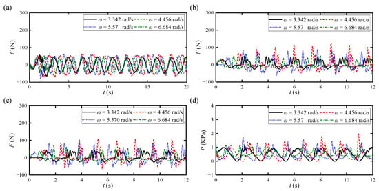
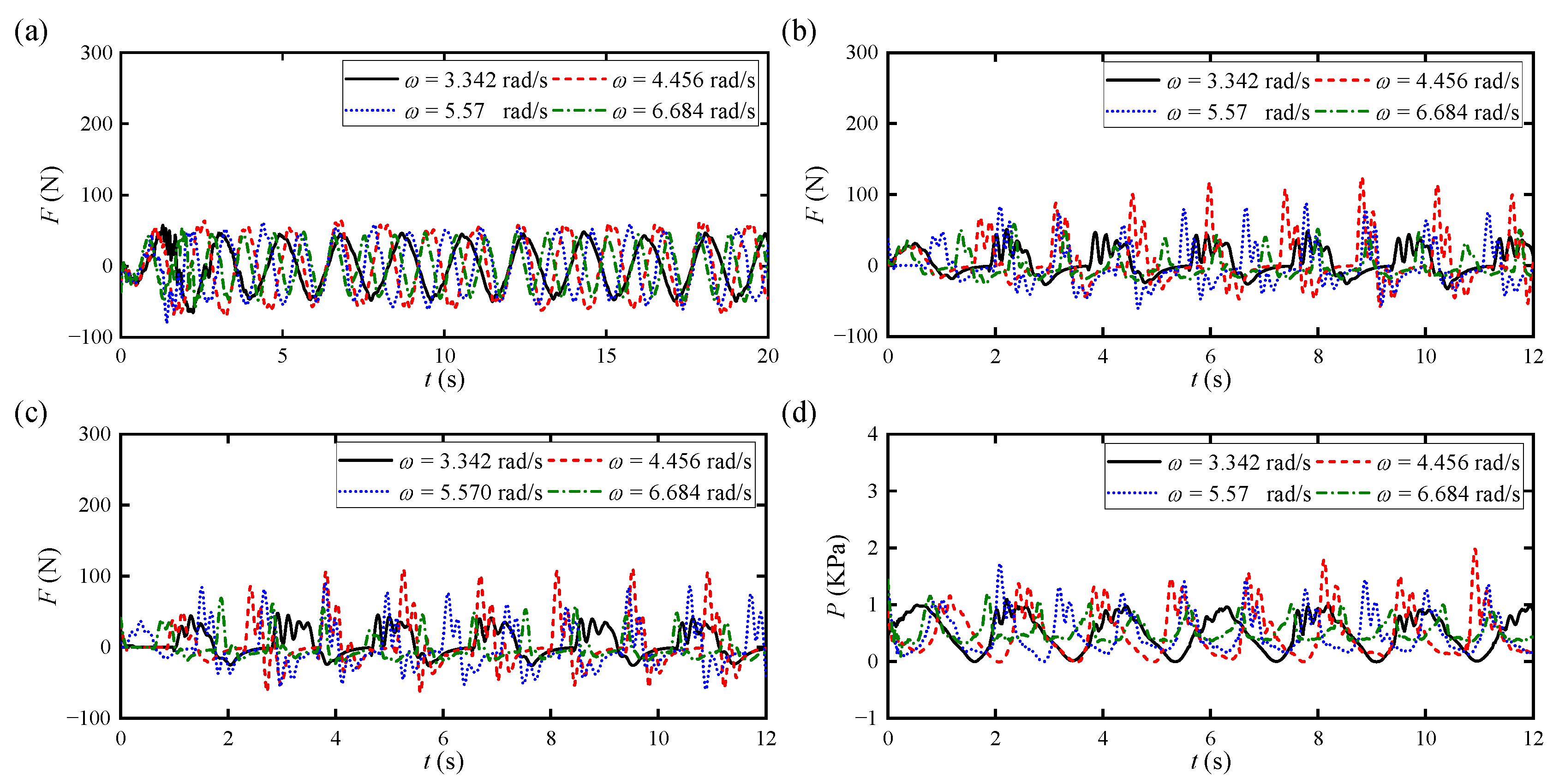
We finally plot the various curves of $F_1$, $F_2$, $F_3$, and $P$ versus $t$ under different $\omega$ with multiple elastic baffles, as illustrated in Figure 21a–c and Figure 21d, respectively. It can be observed from the above four figures that $F_1$, acting on the elastic baffle B1, exhibits a characteristic change consistent with $D_1$, which further indicates that the motion state of the elastic baffle directly affects its force characteristics. The dynamic forces (namely $F_2$, $F_3$) acting on the horizontal elastic baffles B2 and B3 exhibit significant nonlinear characteristics and reach their maximum values at $\omega =4.456 \mathrm{r}\mathrm{a}\mathrm{d}/\mathrm{s}$. Additionally, as illustrated in Figure 21d, $P$ does not increase linearly with $\omega$. In contrast, when $\omega$ approaches ${\omega }_1=4.456$ $\mathrm{r}\mathrm{a}\mathrm{d}/\mathrm{s}$, $P$ reaches its maximum value. Quantitatively, the peak impact pressure surges to 2.0 kPa at $\omega =4.456 \mathrm{r}\mathrm{a}\mathrm{d}/\mathrm{s}$, exhibiting an increase of 100% relative to the non-resonant high-frequency excitation ($\omega =3.342 \mathrm{r}\mathrm{a}\mathrm{d}/\mathrm{s}$).

Figure 21. Various curves of $F_1$, $F_2$, $F_3$ and $P$ versus $t$ under different $w$ with single elastic baffle: (a) $F_1$; (b) $F_2$; (c) $F_3$; (d) $P$.

4.2.2. Influence of $\mathit{\theta }$

We specifically conduct numerical simulations under $\theta =4^{\mathrm{o}}$, $5^{\mathrm{o}}$, $6^{\mathrm{o}}$, and $7^{\mathrm{o}}$, while keeping $\omega =4.456$ $\mathrm{r}\mathrm{a}\mathrm{d}/\mathrm{s}$ and $h/h_b=1.25$ constant to investigate the influence of $\theta$ on the interaction between the sloshing and the multiple elastic baffles. We first plot the various curves of ${\eta }_1$ and ${\eta }_2$ versus $t$ under different $\theta$ with multiple elastic baffles, as illustrated in Figure 22a and Figure 23a, respectively. It can be observed from the above two figures that under different $\theta$ with multiple elastic baffles, the overall evolution characteristics of the sloshing remain consistent; as $\theta$ increases, the amplitudes of ${\eta }_1$ and ${\eta }_2$ show a significant increasing trend, and when $\theta =6^{\mathrm{o}}$ and $7^{\mathrm{o}}$, the amplitudes of ${\eta }_1$ and ${\eta }_2$ are relatively close. This phenomenon indicates that the dynamic behavior of the sloshing is greatly affected by the nonlinear effects of $\theta$. Furthermore, we plot the magnitude of ${\eta }_1$ and ${\eta }_2$ under different $\theta$ with multiple elastic baffles using FFT analysis, as illustrated in Figure 22b and Figure 23b, respectively. It can be observed from the above two figures that when $\theta =7^{\mathrm{o}}$, the response amplitudes of ${\eta }_1$ and ${\eta }_2$ reach their maximum, and the results are relatively close between $\theta =6^{\mathrm{o}}$ and $7^{\mathrm{o}}$.

Figure 22. Numerical results for ${\eta }_1$ under different $\theta$ with multiple elastic baffles: (a) various curves of ${\eta }_1$ versus $t$; (b) corresponding FFT analysis of ${\eta }_1$.

Figure 23. Numerical results for ${\eta }_2$ under different $\theta$ with multiple elastic baffles: (a) various curves of ${\eta }_2$ versus $t$; (b) corresponding FFT analysis of ${\eta }_2$.

We next plot the various curves of $D_1$, $D_2$, $D_3$ versus $t$ and the corresponding FFT analysis results of $D_1$, $D_2$, $D_3$ under different $\theta$ with multiple elastic baffles, as illustrated in Figure 24a, Figure 25a, Figure 26a and Figure 24b, Figure 25b, Figure 26b, respectively. The results demonstrate that the amplitude of $D_1$ under $\theta =7^{\mathrm{o}}$ is more significant than that under other $\theta$, exhibiting more severe sloshing response characteristics. The FFT analysis results in Figure 24b further confirm this trend, with the baffle reaching its maximum bending response amplitude at $\theta =7^{\mathrm{o}}$. Additionally, from Figure 25a and Figure 26a, the results demonstrate that the change in $\theta$ has a notable influence on $D_2$ and $D_3$. Specifically, the amplitude of $D_2$ and $D_3$ shows a clear positive correlation trend with $\theta$. Through FFT analysis in Figure 19b and Figure 20b, we can observe that the magnitudes of $D_2$ and $D_3$ both increase notably with increasing $\theta$.

Figure 24. Numerical results for $D_1$ under different $\theta$ with multiple elastic baffles: (a) various curves of $D_1$ versus $t$; (b) corresponding FFT analysis of $D_1$.

Figure 25. Numerical results for $D_2$ under different $\theta$ with multiple elastic baffles: (a) various curves of $D_2$ versus $t$; (b) corresponding FFT analysis of $D_2$.

Figure 26. Numerical results for $D_3$ under different $\theta$ with multiple elastic baffles: (a) various curves of $D_3$ versus $t$; (b) corresponding FFT analysis of $D_3$.

We finally plot the various curves of $F_1$, $F_2$, $F_3$, and $P$ versus $t$ under different $\theta$ with multiple elastic baffles, as illustrated in Figure 27a–c and Figure 27d, respectively. It can be observed from the above four figures that $F_1$, acting on the elastic baffle B1, exhibits a characteristic change consistent with $D_1$, which further indicates that the motion state of the elastic baffle directly affects its force characteristics. The dynamic forces (namely $F_2$, $F_3$) acting on the horizontal elastic baffles B2 and B3 exhibit significant nonlinear characteristics and reach their maximum values at $\theta =7^{\mathrm{o}}$. Additionally, as illustrated in Figure 27d, $P$ also shows a positive correlation growth trend with $\theta$.

Figure 27. Various curves of $F_1$, $F_2$, $F_3$ and $P$ versus $t$ under different $\theta$ with a single elastic baffle: (a) $F_1$; (b) $F_2$; (c) $F_3$; (d) $P$.

4.2.3. Influence of $\mathit{h}/{\mathit{h}}_{\mathit{b}}$

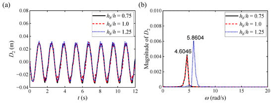
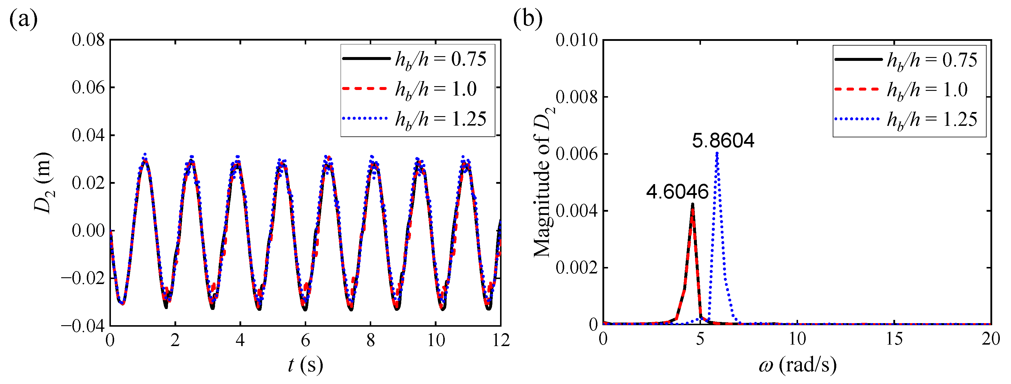
We specifically conduct numerical simulations under $h/h_b=0.75$, $1.0$, and $1.25$, while keeping $\omega =4.456$ $\mathrm{r}\mathrm{a}\mathrm{d}/\mathrm{s}$ and $\theta =4^{\mathrm{o}}$ constant to investigate the influence of $h/h_b$ on the interaction between the sloshing and the multiple elastic baffles. We first plot the various curves of ${\eta }_1$ and ${\eta }_2$ versus $t$ under different $h/h_b$ with multiple elastic baffles, as illustrated in Figure 28a and Figure 29a, respectively. It can be observed from the above two figures that under different $h/h_b$ with multiple elastic baffles, the amplitudes of ${\eta }_1$ and ${\eta }_2$ are relatively close when $h/h_b=0.75$ and $1.0$ and gradually decrease when $h/h_b=1.25$. Furthermore, we plot the magnitude of ${\eta }_1$ and ${\eta }_2$ under different $h/h_b$ with multiple elastic baffles using FFT analysis, as illustrated in Figure 28b and Figure 29b, respectively. The results demonstrate that the magnitude of ${\eta }_1$ and ${\eta }_2$ are relatively close when $h/h_b=0.75$ and $1.0$, which is consistent with Figure 28a and Figure 29a. The motion response of the sloshing occurs at $\omega =4.39603$ and $9.73407$ $\mathrm{r}\mathrm{a}\mathrm{d}/\mathrm{s}$, which are close to ${\omega }_1$ and twice ${\omega }_1$. Additionally, when $\omega =4.39603 \mathrm{r}\mathrm{a}\mathrm{d}/\mathrm{s}$, the maximum amplitudes of ${\eta }_1$ and ${\eta }_2$ occur at $h/h_b=0.75$; while $\omega =9.73407 \mathrm{r}\mathrm{a}\mathrm{d}/\mathrm{s}$, the maximum amplitudes of ${\eta }_1$ and ${\eta }_2$ occur at $h/h_b=1.0$ and gradually decrease with the increase in $h/h_b$.

Figure 28. Numerical results for ${\eta }_1$ under different $h/h_b$ with multiple elastic baffles: (a) various curves of ${\eta }_1$ versus $t$; (b) corresponding FFT analysis of ${\eta }_1$.

Figure 29. Numerical results for ${\eta }_2$ under different $h/h_b$ with multiple elastic baffles: (a) various curves of ${\eta }_2$ versus $t$; (b) corresponding FFT analysis of ${\eta }_2$.

We next plot the various curves of $D$ versus $t$ and the corresponding FFT analysis results of $D$ under different $h/h_b$ with multiple elastic baffles, as illustrated in Figure 30a, Figure 31a, Figure 32a and Figure 30b, Figure 32b, Figure 32b, respectively. The results demonstrate that with the increase in $h/h_b$, $D_1$ gradually decreases, and the two show a negative correlation; the change in $h/h_b$ has no significant effect on the displacement of $D_2$ and $D_3$. The FFT analysis results in Figure 30b, Figure 31b and Figure 32b can further verify the above conclusions.

Figure 30. Numerical results for $D_1$ under different $h/h_b$ with multiple elastic baffles: (a) various curves of $D_1$ versus $t$; (b) corresponding FFT analysis of $D_1$.

Figure 31. Numerical results for $D_2$ under different $h/h_b$ with multiple elastic baffles: (a) various curves of $D_2$ versus $t$; (b) corresponding FFT analysis of $D_2$.

Figure 32. Numerical results for $D_3$ under different $h/h_b$ with multiple elastic baffles: (a) various curves of $D_3$ versus $t$; (b) corresponding FFT analysis of $D_3$.

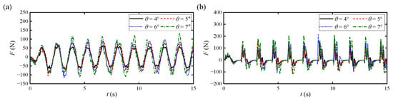
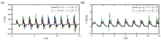
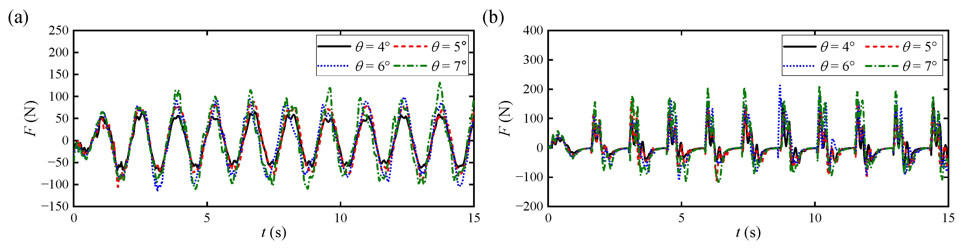
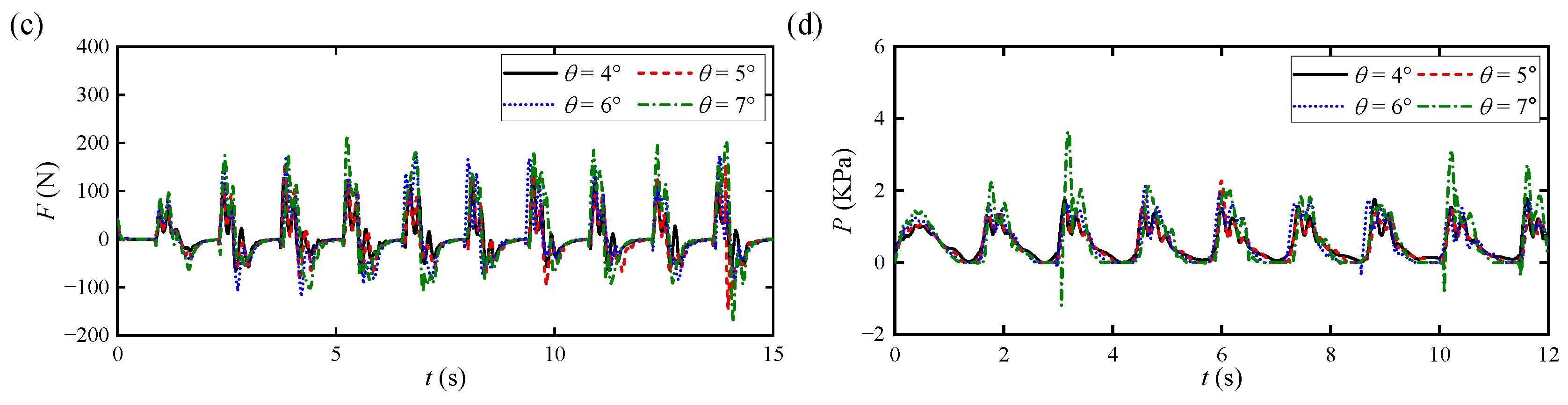
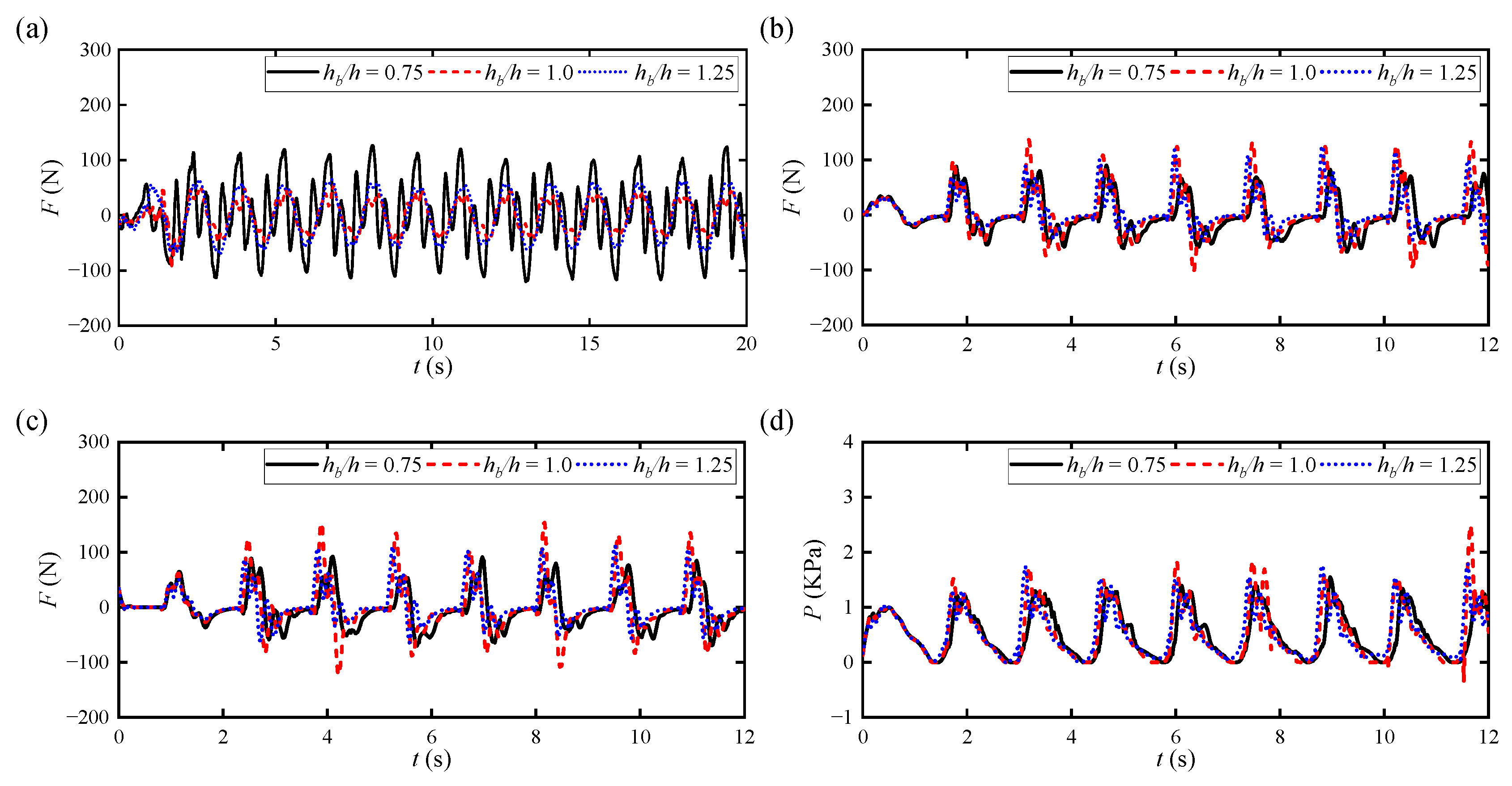
We finally plot the various curves of $F_1$, $F_2$, $F_3$, and $P$ versus $t$ under different $h/h_b$ with multiple elastic baffles, as illustrated in Figure 33a–c and Figure 33d, respectively. It can be observed from the above four figures that $F_1$, acting on the elastic baffle B1, exhibits a characteristic change consistent with $D_1$, which further indicates that the motion state of the elastic baffle directly affects its force characteristics. The dynamic forces (namely $F_2$, $F_3$) acting on the horizontal elastic baffles B2 and B3 exhibit significant nonlinear characteristics and are less affected by changes in $h/h_b$. Additionally, as illustrated in Figure 27d, $P$ is also less affected by changes in $h/h_b$, indicating that $h/h_b$ is not a key factor that can notably change the magnitude of $P$.

Figure 33. Various curves of $F_1$, $F_2$, $F_3$ and $P$ versus $t$ under different $h/h_b$ with multiple elastic baffles: (a) $F_1$; (b) $F_2$; (c) $F_3$; (d) $P$.

5. Conclusions

In this study, an improved SPH method was employed to systematically investigate the hydro-elastic interaction mechanisms between fluid sloshing and elastic baffles in a shaking tank. By analyzing the dynamic responses under varying excitation frequencies ($\omega$), shaking angles ($\theta$), and immersion ratios ($h/h_b$) for both single and multiple baffle configurations, the following key insights into the underlying physical mechanisms are synthesized:

(1)

Hydro-Elastic Damping Mechanism: This study reveals that elastic baffles suppress severe sloshing not merely through physical blockage but via a coupled hydro-elastic damping mechanism. The continuous bending deformation of the baffles effectively absorbs fluid kinetic energy and converts it into structural strain energy. Furthermore, the dynamic boundary alterations introduced by the oscillating baffles disrupt the periodic phase of the fluid wave, preventing the formation of a stable, locked-in resonance.

(2)

Resonance Modulation by Multiple Baffles: Fluid–structure dynamic responses (including free surface elevations, structural displacements, and wall impact pressures) exhibit strong frequency dependence. Under the single-baffle condition, responses universally peak when the external excitation frequency ($\omega$) approaches the tank’s resonant frequency (${\omega }_1=4.456$ $\mathrm{r}\mathrm{a}\mathrm{d}/\mathrm{s}$), yielding peak displacements and impact pressures that are up to 2.0 times higher than those observed under off-resonance conditions. However, the introduction of multiple elastic baffles significantly alters the internal geometry, effectively shifting the resonance response to higher frequency bands.

(3)

Overarching Parametric Trends: Instead of isolated effects, the system exhibits coupled nonlinear responses to external variables. The shaking angle ($\theta$) acts as a clear amplification factor, uniformly intensifying free surface elevations, structural deformations, and impact pressures. Conversely, the immersion ratio ($h/h_b$) governs the effective damping depth; increasing $h/h_b$ generally attenuates structural displacements and impact pressures, exhibiting a negative correlation with dynamic loads.

In summary, this study explicitly correlates the external excitation conditions with the inherent resonance characteristics of the fluid–structure system. The revealed mechanisms provide a solid theoretical foundation for designing flexible internal structures to suppress severe hydrodynamic impacts in liquid-storage tanks.

Furthermore, the mechanistic analysis demonstrates that the superior sloshing suppression capability of the elastic baffle originates not merely from passive obstruction but from two synergistic physical mechanisms: (i) the reversible conversion of fluid kinetic energy into structural strain energy during bending deformation, and (ii) the phase-lagged structural response that actively desynchronizes incident wave motion and suppresses resonant amplification—thereby establishing a fundamentally distinct hydro-elastic damping paradigm relative to conventional rigid blockages.

References

- Steinbrugge, K.V.; Rodrigo, F.A. The Chilean earthquakes of May 1960: A structural engineering viewpoint. Bull. Seismol. Soc. Am. 1963, 53, 225–307. [Google Scholar] [CrossRef] [Scilit]
- Knarr, M.; Gersdorff, N.V.; Duron, Z.; Yen, J. The investigation of a concrete gravity dam in a narrow canyon using 3-D non-linear analysis. In Proceedings of the 21st Century Dam Design-Advances and Adaptations, 31st Annual USSD Conference, San Diego, CA, USA, 11–15 April 2011. [Google Scholar]
- Malhotra, P.K. Sloshing loads in tanks with insufficient freeboard. Earthq. Spectra 2005, 4, 1185–1192. [Google Scholar] [CrossRef] [Scilit]
- Cho, J.R.; Lee, H.W. Numerical study on liquid sloshing in baffled tank by nonlinear finite element method. Comput. Methods Appl. Mech. Eng. 2004, 193, 2581–2598. [Google Scholar] [CrossRef] [Scilit]
- Akyildiz, H.; Ünal, E. Experimental investigation of pressure distribution on a rectangular tank due to the liquid sloshing. Ocean Eng. 2005, 32, 1503–1516. [Google Scholar] [CrossRef] [Scilit]
- Liu, D.M.; Lin, P.Z. Three-dimensional liquid sloshing in a tank with baffles. Ocean Eng. 2009, 36, 202–212. [Google Scholar] [CrossRef] [Scilit]
- Xue, M.A.; Zheng, J.; Lin, P.Z.; Yuan, X.L. Experimental study on vertical baffles of different configurations in suppressing sloshing pressure. Ocean Eng. 2017, 136, 178–189. [Google Scholar] [CrossRef] [Scilit]
- Chu, C.R.; Wu, Y.R.; Wu, T.R.; Wang, C.Y. Slosh-induced hydrodynamic force in a water tank with multiple baffles. Ocean Eng. 2018, 167, 282–292. [Google Scholar] [CrossRef] [Scilit]
- Nasar, T.; Sannasiraj, S.A. Sloshing dynamics and performance of porous baffle arrangements in a barge carrying liquid tank. Ocean Eng. 2019, 183, 24–39. [Google Scholar] [CrossRef] [Scilit]
- Yu, L.; Xue, M.A.; Jiang, Z. Experimental investigation of parametric sloshing in a tank with vertical baffles. Ocean Eng. 2020, 213, 107783. [Google Scholar] [CrossRef] [Scilit]
- Zang, Q.; Fang, H.; Liu, J.; Lin, G. Boundary element model for investigation of the effects of various porous baffles on liquid sloshing in the two-dimensional rectangular tank. Eng. Anal. Bound. Elem. 2019, 108, 484–500. [Google Scholar] [CrossRef] [Scilit]
- Paik, K.J.; Carrica, P.M. Fluid–structure interaction for an elastic structure interacting with free surface in a rolling tank. Ocean Eng. 2014, 84, 201–212. [Google Scholar] [CrossRef] [Scilit]
- Hwang, S.C.; Park, J.C.; Gotoh, H.; Abbas, K.; Kang, K.J. Numerical simulations of sloshing flows with elastic baffles by using a particle-based fluid–structure interaction analysis method. Ocean Eng. 2016, 118, 227–241. [Google Scholar] [CrossRef] [Scilit]
- Maiti, P.R.; Bhattacharyya, S.K. Liquid-structure interaction coupled motion of a cantilever plate inside a container an experimental investigation. Int. J. Fluid Mech. Res. 2020, 47, 517–531. [Google Scholar] [CrossRef] [Scilit]
- Cho, I.H. Liquid sloshing in a swaying/rolling rectangular tank with a flexible porous elastic baffle. Mar. Struct. 2021, 75, 102865. [Google Scholar] [CrossRef] [Scilit]
- Cao, Z.; Xue, M.A.; Yuan, X.; Zheng, J. A fast semi-analytic solution of liquid sloshing in a 2-D tank with dual elastic vertical baffles and walls. Ocean Eng. 2023, 273, 113951. [Google Scholar] [CrossRef] [Scilit]
- Ren, Y.R.; Khayyer, A.; Lin, P.Z.; Hu, X.Y. Numerical modeling of sloshing flow interaction with an elastic baffle using SPHinXsys. Ocean Eng. 2023, 267, 113110. [Google Scholar] [CrossRef] [Scilit]
- Ren, Y.R.; Xue, M.A.; Lin, P.Z. Experimental study of sloshing characteristics in a rectangular tank with elastic baffles. J. Fluids Struct. 2023, 122, 103984. [Google Scholar] [CrossRef] [Scilit]
- Khayyer, A.; Gotoh, H.; Falahaty, H.; Shimizu, Y. Towards development of enhanced fully-Lagrangian mesh-free computational methods for fluid-structure interaction. J. Hydrodyn. 2018, 30, 49–61. [Google Scholar] [CrossRef] [Scilit]
- Sun, P.N.; Le Touze, D.; Oger, G.; Zhang, A.M. An accurate FSI-SPH modeling of challenging fluid-structure interaction problems in two and three dimensions. Ocean Eng. 2021, 221, 108552. [Google Scholar] [CrossRef] [Scilit]
- Lo, E.Y.M.; Shao, S. Simulation of near-shore solitary wave mechanics by an incompressible SPH method. Appl. Ocean Res. 2002, 24, 275–286. [Google Scholar] [CrossRef] [Scilit]
- Gotoh, H. Sub-particle-scale turbulence model for the MPS method-Lagrangian flow model for hydraulic engineering. Int. J. Comput. Fluid Dyn. 2001, 9, 339–347. [Google Scholar]
- Dalrymple, R.A.; Rogers, B.D. Numerical modeling of water waves with the SPH method. Coast. Eng. 2006, 53, 141–147. [Google Scholar] [CrossRef] [Scilit]
- Molteni, D.; Colagrossi, A. A simple procedure to improve the pressure evaluation in hydrodynamic context using the SPH. Comput. Phys. Commun. 2009, 180, 861–872. [Google Scholar] [CrossRef] [Scilit]
- Ganzenmüller, G.C. An hourglass control algorithm for Lagrangian smooth particle hydrodynamics. Comput. Methods Appl. Mech. Eng. 2015, 286, 87–106. [Google Scholar] [CrossRef] [Scilit]
- Crespo, A.J.C.; Gómez-Gesteira, R.; Dalrymple, R.A. Boundary conditions generated by dynamic particles in SPH methods. Comput. Mater. Contin. 2007, 5, 173–184. [Google Scholar]
- Leimkuhler, B.J.; Matthews, C. Molecular Dynamics; Springer International Publishing: New York, NY, USA, 2016. [Google Scholar]
- Faltinsen, O.M. A numerical nonlinear method of sloshing in tanks with two-dimensional flow. J. Ship Res. 1978, 22, 193–202. [Google Scholar] [CrossRef] [Scilit]
- Zhang, C.; Li, Y.; Meng, Q. Fully nonlinear analysis of second-order sloshing resonance in a three-dimensional tank. Comput. Fluids 2015, 116, 88–104. [Google Scholar] [CrossRef] [Scilit]
Disclaimer/Publisher’s Note: The statements, opinions and data contained in all publications are solely those of the individual author(s) and contributor(s) and not of MDPI and/or the editor(s). MDPI and/or the editor(s) disclaim responsibility for any injury to people or property resulting from any ideas, methods, instructions or products referred to in the content. |
© 2026 by the authors. Licensee MDPI, Basel, Switzerland. This article is an open access article distributed under the terms and conditions of the Creative Commons Attribution (CC BY) license.