A Short-Term Load and Photovoltaic Power Forecasting Method Based on Robust Data Preprocessing and QPSO-BiLSTM

Abstract

Accurate short-term load and photovoltaic (PV) power forecasting is essential for power-system dispatch and renewable-energy accommodation under high PV penetration. However, measured source-load data often contain outliers and missing values, while the forecasting performance of bidirectional long short-term memory (BiLSTM) networks is sensitive to hyperparameter selection. This paper develops an integrated short-term load and PV power forecasting framework that combines characteristic-aware robust data preprocessing with BiLSTM modeling tuned by quantum particle swarm optimization (QPSO). An iterative 3σ criterion is first used to detect spike, drop, negative, and flat anomalies according to the different characteristics of load and PV data, and piecewise cubic Hermite interpolation is then applied to repair abnormal and missing points. A BiLSTM network is used to capture bidirectional temporal dependencies, and QPSO is introduced to optimize the number of hidden units, maximum training epochs, and learning rate. Experiments were conducted on measured load and PV datasets with a 15 min resolution, and the proposed model was compared with long short-term memory (LSTM), BiLSTM, and a BiLSTM tuned by particle swarm optimization (PSO), denoted PSO-BiLSTM. In the primary forecasting evaluation on measured grid data, QPSO-BiLSTM achieved mean absolute percentage error (MAPE) values of 2.1616% for load forecasting and 7.5687% for PV power forecasting. Additional random-seed-controlled ablation and robustness validation confirmed statistically significant contributions of the preprocessing procedure and QPSO to load forecasting, while the proposed framework maintained competitive performance for PV forecasting. The proposed method improves forecasting accuracy and provides reliable data support for short-term operation and dispatch of renewable-energy power systems.

1. Introduction

Against the background of global low-carbon energy transition and the development of new power systems, renewable energy represented by photovoltaic (PV) generation has been widely integrated into modern power systems [1,2]. PV generation is clean, low-carbon, and broadly deployable, making it an important technical pathway for promoting the green transformation of the energy sector [3,4]. However, compared with conventional fossil-fuel generation units, PV output is strongly affected by solar irradiance, ambient temperature, cloud movement, and weather variations, and therefore exhibits intermittency, volatility, and randomness [5,6,7]. At the same time, load demand on the user side is influenced by temperature variation, production and living patterns, social activities, and electricity consumption behavior, showing nonlinear and non-stationary characteristics [8,9,10]. The combined uncertainty of source-side PV generation and demand-side load increases the difficulty of power balancing, reserve allocation, and short-term operation scheduling. Therefore, accurate short-term load and PV power forecasting is of great significance for maintaining power system security, improving renewable energy accommodation, and supporting optimal dispatch decisions [11,12].

Short-term load forecasting and PV power forecasting have become important research topics in the operation and optimization of renewable-energy power systems [13]. Existing forecasting methods can generally be divided into physical modeling methods, statistical methods, and data-driven methods [2]. Physical models are usually established according to PV module mechanisms, geographical location, irradiance, and temperature. Although they provide a certain degree of interpretability, they require complete meteorological and equipment parameters, involve complex modeling processes, and may have limited applicability across different regions and operating conditions. Statistical methods, such as linear regression, time-series analysis, autoregressive moving average models, and exponential smoothing models, have simple structures and high computational efficiency [14,15,16]. However, load and PV power series usually involve strong nonlinearity, multi-factor coupling, and short-term fluctuations. Traditional statistical methods are often insufficient for capturing complex temporal patterns, and their forecasting accuracy may decrease under highly volatile conditions.

With the development of artificial intelligence, machine learning and deep learning methods have become important tools for power time-series forecasting [17]. Compared with traditional models, deep learning models can automatically extract high-level features from input data through multilayer nonlinear structures and show strong capability in representing complex nonlinear relationships. Convolutional neural networks (CNNs) are commonly used for local feature extraction, while recurrent neural networks (RNNs) and their variants are more suitable for sequential data modeling. Long short-term memory (LSTM) networks use input gates, forget gates, and output gates to regulate information flow and alleviate the gradient vanishing problem of traditional RNNs [18]. As a result, LSTM models have been widely applied in short-term load forecasting, PV power forecasting, and renewable energy output prediction [19,20,21]. Bidirectional long short-term memory (BiLSTM) networks further introduce both forward and backward information transmission directions, enabling the model to extract historical and contextual temporal features simultaneously and thereby improving its ability to model complex sequential patterns [22,23].

In recent years, deep-learning-based load and PV power forecasting has increasingly evolved toward hybrid architectures that combine complementary feature-extraction and temporal-modeling mechanisms. Improved BiLSTM, CNN-LSTM, CNN-BiLSTM-attention, and attention-enabled Transformer models have been developed to enhance the representation of nonlinear temporal patterns and influential variables [24,25,26,27]. Multitask and probabilistic deep-learning approaches have further extended forecasting from deterministic point estimation to the characterization of prediction uncertainty [28,29]. These advances have improved the modeling capability of forecasting networks, while their performance remains strongly dependent on the quality of the input data and the configuration of model hyperparameters. In measured power-system data, abnormal observations caused by acquisition or transmission errors can distort the temporal patterns used for model training, making data-quality control an important part of the forecasting pipeline [30].

Data preprocessing directly affects the information presented to forecasting models. Existing power-data studies have used statistical detection, interpolation, and related cleaning techniques to identify abnormal observations and improve the quality of model inputs [30]. The design of such preprocessing is particularly important when different types of power-series data are considered within the same forecasting framework. Load power generally varies continuously throughout the day, whereas PV power is naturally zero at night and exhibits weather-driven fluctuations during daylight hours. Consequently, using the same statistical population to detect anomalies in both series can distort the reference distribution: nighttime zeros can strongly affect the mean and variance of PV data, while the intra-day variation pattern of load data follows a different operating structure. This difference motivates an anomaly-detection strategy in which the statistical reference is constructed according to the physical characteristics of each forecasting object.

Hyperparameter configuration is another major factor governing the forecasting performance of recurrent neural networks. The number of hidden units, training epochs, learning rate, and related settings directly affect representation capacity, convergence behavior, and generalization. Metaheuristic algorithms have therefore been widely investigated for automated hyperparameter selection in load-forecasting models [31]. Among them, particle swarm optimization (PSO) is attractive because of its simple search mechanism and straightforward implementation, although loss of swarm diversity can lead to premature convergence in complex search spaces [32,33]. Quantum particle swarm optimization (QPSO) replaces the conventional velocity-based update with a probabilistic position-update mechanism derived from quantum behavior, thereby providing a different exploration mechanism for global parameter search [34].

Recent studies have also broadened the evaluation of short-term power forecasting beyond network architecture alone. A hybrid one-dimensional convolutional neural network-gated recurrent unit (1D CNN-GRU) model combined Shapley additive explanations (SHAP)-based feature selection, exponential moving-average smoothing, and Gaussian-noise augmentation for short-term PV forecasting, achieving the lowest root mean square error (RMSE) across three seasonal test cases and the shortest training time among the deep-learning models evaluated in that study [35]. A multimodal PV forecasting framework based on satellite images and time-series data further incorporated robust feature fusion to reduce sensitivity to noise and missing observations while maintaining low model complexity [36]. For short-term customer-load forecasting, causal inference has been introduced to reduce performance degradation associated with customer heterogeneity and distribution drift, extending model assessment from fitting accuracy to generalization across changing data characteristics [37]. These studies indicate that forecasting accuracy, computational efficiency, robustness to imperfect data, and generalization are increasingly evaluated as complementary aspects of forecasting performance.

Closely related studies have also integrated particle-swarm optimization with recurrent forecasting networks. Liu et al. used density-based spatial clustering of applications with noise (DBSCAN) and support vector machine (SVM) for data cleaning and combined the preprocessing scheme with PSO-LSTM for short-term PV power prediction, reporting additional error reduction after the cleaned data were used for model training [38]. Lin et al. decomposed PV and meteorological series, extracted key features, and employed an improved-PSO-optimized BiLSTM for PV power forecasting [39]. Peng et al. combined symplectic geometry mode decomposition and kernel principal component analysis with PSO-BiLSTM for wind and PV power prediction [40]. Similar optimizer-assisted recurrent frameworks have been developed for load forecasting: Ma et al. integrated CNN-based feature extraction, moving-average preprocessing, attention, and an LSTM model optimized by improved chaotic particle swarm optimization (ICPSO) for short-term household load forecasting [41]. Raju et al. used chaotic PSO to jointly tune hidden neurons, learning rate, batch size, dropout rate, and activation function of an LSTM model for short-term solar-irradiance forecasting [42]. More recently, QPSO-enhanced LSTM has been embedded in a hybrid load-forecasting framework combining optimized variational mode decomposition and GRU/LSTM modeling [43]. Collectively, these studies establish optimizer-assisted LSTM/BiLSTM and preprocessing-plus-optimization pipelines as established methodological directions; their substantive differences arise from how the input data are processed, how temporal information is represented, which parameters are optimized, and how the complete forecasting framework is validated. Against this background, the present study focuses on constructing anomaly-detection statistics separately for load and PV according to their physical operating patterns and integrating this preprocessing with bidirectional temporal modeling and QPSO-based hyperparameter optimization within the same forecasting framework.

Taken together, the literature points to three issues that remain relevant to joint load and PV forecasting. First, existing data-quality methods can identify abnormal observations, suppress noise, or repair incomplete inputs [30,36,38], but the statistical reference used for anomaly detection is generally designed for a specific forecasting object. A unified source-load framework requires the detection statistics themselves to reflect the continuous daily behavior of load and the nighttime-zero constraint of PV generation. Second, the closely related studies reviewed in [38,39,40,41,42,43] mainly employ preprocessing for data cleaning, signal decomposition, feature extraction, or input enhancement before recurrent forecasting, whereas they do not construct separate anomaly-detection reference populations for load and PV according to their distinct operating characteristics and integrate this design with bidirectional temporal modeling within the same forecasting framework. Third, hybrid forecasting pipelines combine several interacting modules, making component-wise ablation, random-seed-controlled robustness validation, and computational-cost evaluation necessary to quantify the contribution and cost of each stage and to complement the primary forecasting evaluation on measured grid data. These issues motivate an integrated forecasting framework that links characteristic-aware data preprocessing, bidirectional temporal feature extraction, adaptive hyperparameter optimization, and systematic validation for both load and PV power.

To address these issues, this paper develops an integrated short-term load and PV power forecasting framework that combines characteristic-aware data preprocessing with QPSO-tuned BiLSTM modeling. For data-quality control, an iterative 3σ criterion is implemented with different statistical populations for load and PV data to detect spike, drop, negative, and flat anomalies, after which piecewise cubic Hermite interpolation is used to repair abnormal and missing points. The cleaned sequences are then modeled by BiLSTM to capture bidirectional temporal dependencies, while QPSO adaptively determines the number of hidden units, maximum training epochs, and learning rate. The framework is evaluated on both load and PV forecasting tasks through baseline comparisons on measured grid data and random-seed-controlled component-wise ablation and robustness validation. In addition to RMSE, mean absolute error (MAE), mean absolute percentage error (MAPE), and R², the computational time required for hyperparameter search, final-model training, and inference is reported to characterize the accuracy–cost profile of the optimization stage.

The main contributions of this paper are as follows:

(1)

A characteristic-aware preprocessing strategy is developed for heterogeneous load and PV measurements. The anomaly-detection statistics are constructed differently for the two forecasting objects: a within-day statistical population is used for load data, whereas nonzero observations at the same time slot across different days are used for PV data. Iterative 3σ detection is then combined with piecewise cubic Hermite interpolation polynomial (PCHIP)-based repair to process spike, drop, negative, flat, and missing observations while preserving the operating characteristics of the two series.

(2)

A unified load/PV forecasting pipeline is constructed by coupling the characteristic-aware preprocessing strategy with QPSO-tuned BiLSTM modeling. The methodological distinction lies in applying forecasting-object-specific data-quality control before bidirectional temporal modeling and adaptive hyperparameter optimization, allowing the same framework to accommodate the different operating characteristics of load and PV power series.

(3)

The framework is evaluated in both load and PV forecasting scenarios through comparative forecasting experiments on measured grid data, random-seed-controlled component-wise ablation and robustness validation, and computational-time analysis. The evaluation quantifies the contributions of preprocessing, bidirectional temporal modeling, and QPSO-based hyperparameter optimization while separately characterizing measured-data forecasting performance, robustness across random seeds, and the computational cost introduced by optimization.

The remainder of this paper is organized as follows: Section 2 introduces the data preprocessing method, the BiLSTM network structure, the QPSO algorithm, and the QPSO-BiLSTM forecasting procedure. Section 3 presents the experimental data, input and output settings, evaluation metrics, and comparison models. Section 4 analyzes and discusses the load forecasting and PV power forecasting results. Section 5 concludes the paper and outlines future research directions.

2. Robust Data Preprocessing and QPSO-BiLSTM Forecasting Methodology

To improve the forecasting accuracy of short-term load and photovoltaic (PV) power, this study develops an integrated forecasting framework that combines characteristic-aware robust data preprocessing, BiLSTM-based bidirectional temporal feature extraction, and QPSO-based adaptive hyperparameter optimization. The overall methodology consists of four parts. First, the raw load and PV power data are preprocessed to detect outliers and repair missing values. Second, a BiLSTM network is constructed to capture the temporal dependence of load and PV power series. Third, quantum particle swarm optimization (QPSO) is introduced to optimize the key hyperparameters of the BiLSTM model. Finally, the optimized model is used to perform short-term load and PV power forecasting.

2.1. Characteristic-Aware Data Preprocessing for Load and PV Power Data

Measured power-system data are usually collected by sensors and transmitted to data centers through communication networks. During data acquisition, transmission, and storage, sensor faults, communication interruptions, and manual recording errors may introduce missing values and abnormal values into the raw dataset. If these noisy data are directly used for model training, the forecasting model may suffer from increased bias and reduced generalization ability. Therefore, systematic data preprocessing is required before model construction.

In this study, data preprocessing includes two steps: outlier detection and missing value repair. Considering the different physical characteristics of load and PV power data, different detection strategies are adopted. PV power is strictly zero during nighttime and only generated during daytime. If full-day PV data are used for statistical detection, numerous zero values may significantly reduce the mean and standard deviation, causing normal daytime PV output to be misidentified as abnormal. Therefore, PV data are detected using a cross-day same-time-slot strategy, where nonzero values at the same time slot across different days are used as the statistical population. In contrast, load data are continuous throughout the day and show clear intra-day variation. Therefore, load data are detected using a within-day strategy, where the daily load sequence is used as the statistical population.

2.1.1. Iterative 3σ-Based Outlier Detection

The traditional 3σ criterion uses the sample mean μ and standard deviation σ as statistical references and identifies values outside the interval [μ − 3σ, μ + 3σ] as outliers [44]. However, when spike anomalies and drop anomalies coexist in a source-load time series, extreme spike values may increase the estimated mean and standard deviation, resulting in an excessively wide detection interval and missed detection of drop anomalies. To address this problem, an iterative 3σ criterion is adopted in this study.

Let the initial effective sample set be D⁽⁰⁾. At the k-th iteration, μ^(k) and σ^(k) denote the mean and standard deviation of the current effective sample set, respectively, and are calculated as follows:

$${\mu }^{\left(k\right)}={\displaystyle \frac{1}{N_{D^{\left(k\right)}}}}{\displaystyle {\sum }_{x_i\in D^{\left(k\right)}}{x}_i}$$

(1)

$${\sigma }^{\left(k\right)}=\sqrt{{\displaystyle \frac{1}{N_{D^{\left(k\right)}}}}{\displaystyle {\sum }_{x_i\in D^{\left(k\right)}}{\left(x_i-{\mu }^{\left(k\right)}\right)}^2}}$$

(2)

where D^(k) denotes the effective sample set retained after the k-th iteration, x_i is the measured power value at sampling time i, and $N_{D^{\left(k\right)}}$ is the number of samples in D^(k). Compared with a single calculation of the mean and standard deviation, the iterative method gradually removes extreme samples and obtains more robust statistical parameters. When D^(k+1) = D^(k), the iteration stops, and the final μ^* and σ^* denote the robust mean and standard deviation, respectively.

Based on μ^* and σ^*, four types of abnormal data are defined. The corresponding index sets of spike, drop, negative, and flat anomalies are denoted by Ω_spike, Ω_drop, Ω_neg, and Ω_flat, respectively, and the not-a-number value (NaN) is used to denote a missing value.

First, spike anomalies are caused by instantaneous voltage disturbance, measurement overflow, or recording errors, and are represented by abnormally large power values:

Ω_spike = {i|x_i > μ^* + 3σ^*,x_i ≠ NaN}

(3)

Second, drop anomalies are caused by sensor under-range, signal attenuation, or loose wiring, and are represented by abnormally small but nonnegative power values:

Ω_drop = {i|0 ≤ x_i < μ^* − 3σ^*,x_i ≠ NaN}

(4)

Third, negative anomalies are detected according to the physical non-negativity of load and PV power:

Ω_neg = {i|x_i<0,x_i ≠ NaN}

(5)

Fourth, a flat anomaly is defined as a sequence of identical measurements over a continuous window:

Ω_flat = {i|x_i+j = x_i,j = 0,1,…,W − 1,x_i ≠ NaN}

(6)

where W is the length of the sliding window and j denotes the relative offset within the window for flat anomaly detection. After the above abnormal points are detected, their values are set as missing values and merged with the original missing points for subsequent repair.

2.1.2. PCHIP-Based Missing Value Repair

Missing values in source-load time series may appear as isolated points caused by occasional acquisition errors or as continuous segments caused by communication interruptions. To repair both abnormal points and original missing points, piecewise cubic Hermite interpolation polynomial (PCHIP) is used in this study [45].

Assume that a missing segment starts at time s. Let j denote the subinterval index, t the time coordinate, and t_j and t_j+1 the time coordinates of the two endpoints of the j-th subinterval. In each subinterval [t_j,t_j+1], PCHIP constructs the cubic polynomial p_j(t) as follows:

p_j(t) = h₀₀(τ)x_j + h₁₀(τ)m_jΔt + h₀₁(τ)x_j+1 + h₁₁(τ)m_j+1Δt

(7)

$$\tau ={\displaystyle \frac{t-t_j}{t_{j+1}-t_j}}$$

(8)

Δt = t_j+1 − t_j

(9)

where Δt is the width of the current subinterval; τ ∈ [0,1] is the normalized local time coordinate; x_j and x_j+1 are the measured power values at the two endpoints of the subinterval; m_j and m_j+1 are the first-order derivative estimates at the endpoints; and h₀₀, h₁₀, h₀₁, and h₁₁ are Hermite basis functions:

h₀₀(τ) = 2τ³ − 3τ² + 1

(10)

h₁₀(τ) = τ³ − 2τ² + τ

(11)

h₀₁(τ) = −2τ³ + 3τ²

(12)

h₁₁(τ) = τ³ − τ²

(13)

PCHIP constructs independent cubic polynomials in different subintervals and ensures continuity of both the function values and the first-order derivatives at the endpoints. Compared with ordinary high-order polynomial interpolation, PCHIP can better preserve the shape of the original curve and avoid unrealistic overshoot. Accordingly, PCHIP was selected as a shape-preserving repair method that provides a practical balance between local smoothness and suppression of nonphysical overshoot, which is desirable for load and PV power series subject to physical constraints. The derivative estimate at each endpoint is determined based on the local slopes. Let the adjacent slopes be δ_j−1 and δ_j. The derivative estimate is calculated as

$$m_j=\left\{\begin{array}{l}0,{\delta }_{j-1}\cdot {\delta }_j\le 0\\ {\displaystyle \frac{2}{\frac{1}{{\delta }_{j-1}}+\frac{1}{{\delta }_j}}},{\delta }_{j-1}\cdot {\delta }_j>0 \end{array}\right.$$

(14)

where

$${\delta }_j={\displaystyle \frac{x_{j+1}-x_j}{t_{j+1}-t_j}}$$

(15)

Through the above procedure, the detected abnormal values and original missing values are repaired, and complete and physically reasonable load and PV power sequences are obtained for model training.

2.2. BiLSTM-Based Temporal Feature Extraction Model

After data preprocessing, the cleaned load and PV power sequences are used to train the forecasting model. Since load and PV power data are typical time-series data, their future values depend not only on current conditions but also on historical temporal patterns. In this study, BiLSTM is used as the basic forecasting model because it can extract temporal information in both forward and backward directions.

2.2.1. LSTM Network Structure

Recurrent neural networks (RNNs) are designed for sequence modeling, but standard RNNs may suffer from gradient vanishing or gradient explosion when learning long-term dependencies. Long short-term memory (LSTM) networks introduce a cell state and several gate structures to control information flow, effectively improving long-sequence modeling ability [18].

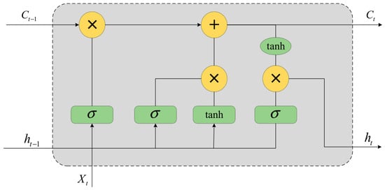
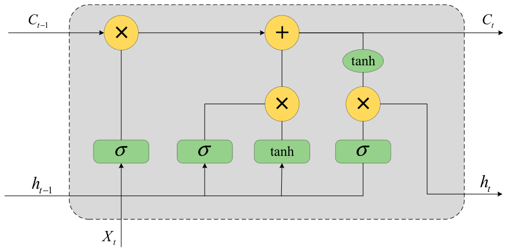
As shown in Figure 1, an LSTM unit contains two main state vectors at time t: the hidden state h_t and the cell state C_t. The information flow is controlled by the forget gate, input gate, and output gate. The forward propagation of an LSTM unit is expressed as follows:

f_t = σ(W_f[h_t−1,x_t] + β_f)

(16)

i_t = σ(W_i[h_t−1,x_t] + β_i)

(17)

$${\tilde{C}}_t=\tanh \left(W_c\left[h_{t-1},x_t\right]+{\beta }_c\right)$$

(18)

$$C_t=f_t{C}_{t-1}+i_t{\tilde{C}}_t$$

(19)

o_t = σ(W_o[h_t−1,x_t] + β_o)

(20)

h_t = o_ttanh(C_t)

(21)

where f_t, i_t, and o_t are the outputs of the forget gate, input gate, and output gate, respectively; C_t and ${\tilde{C}}_t$ denote the cell state and candidate cell state; W_f, W_i, W_c, and W_o are weight matrices; β_f, β_i, β_c, and β_o are bias terms; σ(⋅) is the sigmoid activation function; x_t is the input at time t; and h_t is the hidden output at time t.

Figure 1. LSTM unit structure.

2.2.2. BiLSTM Network Structure

Although LSTM can capture long-term temporal dependencies, its standard structure processes information in only one temporal direction. For time-series forecasting, the target output may be related not only to previous observations but also to contextual information within the input sequence. To better extract bidirectional temporal features, BiLSTM combines a forward LSTM and a backward LSTM in parallel [22].

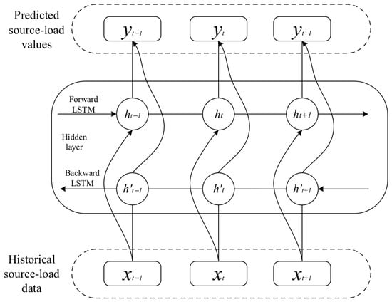
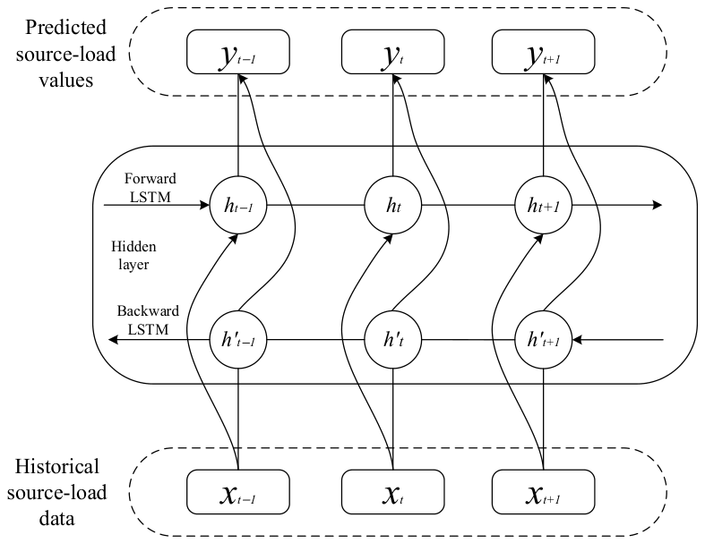
As shown in Figure 2, the forward LSTM processes the input sequence in chronological order to extract historical temporal features, while the backward LSTM processes the sequence in the reverse direction to capture backward contextual information. For each time step, the hidden states of the two directions are calculated separately and then fused to generate the final output. The calculation process of BiLSTM is expressed as follows:

$$\overrightarrow{h_t}=\mathit{LSTM}\left(x_t,\overrightarrow{h_{t-1}}\right)$$

(22)

$$\overleftarrow{h_t}=\mathit{LSTM}\left(x_t,\overleftarrow{h_{t+1}}\right)$$

(23)

$$y_t=W_{\overrightarrow{\mathit{hy}}}\overrightarrow{h_t}+W_{\overleftarrow{\mathit{hy}}}\overleftarrow{h_t}+{\beta }_y$$

(24)

where t denotes the time step; LSTM(⋅) denotes the operation function of the long short-term memory network; $\overrightarrow{h_t}$ denotes the hidden state of the forward LSTM at time t; $\overleftarrow{h_t}$ denotes the hidden state of the backward LSTM at time t; x_t denotes the input source-load feature at time t; $W_{\overrightarrow{\mathit{hy}}}$ denotes the weight coefficient of the forward LSTM; $W_{\overleftarrow{\mathit{hy}}}$ denotes the weight coefficient of the backward LSTM; β_y denotes the bias term of the output layer; and y_t denotes the predicted source-load value at the future time step.

Figure 2. BiLSTM network structure.

In this study, the historical load or PV power sequence is used as the input. The BiLSTM model extracts bidirectional temporal features from the source-load series and maps them to future load or PV power values through the output layer. Compared with a unidirectional LSTM, BiLSTM can use both forward and backward temporal information, which improves its ability to represent nonlinear and non-stationary source-load sequences.

2.3. QPSO-Based Hyperparameter Optimization for BiLSTM

Although BiLSTM has strong temporal feature extraction capability, its forecasting performance depends heavily on hyperparameter configuration. To reduce the uncertainty caused by manual parameter tuning, QPSO is used to optimize the key hyperparameters of the BiLSTM model.

Particle swarm optimization (PSO) is a swarm intelligence optimization algorithm inspired by the social behavior of birds or fish [32]. In PSO, each candidate solution is represented by a particle moving in a multidimensional search space. Each particle has two main attributes: position and velocity. The position represents a candidate solution, and the velocity determines the moving direction and distance in the next iteration. Each particle records its own best historical position, called the personal best, while the best position found by the whole swarm is called the global best.

Assume that the search space is D-dimensional and the swarm contains N particles. Let k denote the iteration index. The velocity and position of the i-th particle in the n-th dimension are updated by

v_in(k + 1) = ω ⋅ v_in(k) + c₁r_1,in(k)[p_in(k) − x_in(k)] + c₂r_2,in(k)[g_n(k) − x_in(k)]

(25)

x_in(k + 1) = x_in(k) + v_in(k + 1)

(26)

where x_in(k) and v_in(k) are the position and velocity of the particle, respectively; ω is the inertia weight; c₁ and c₂ are the cognitive and social learning factors; r_1,in(k) and r_2,in(k) are random numbers uniformly distributed in [0,1]; p_in(k) is the personal best position; and g_n(k) is the global best position.

However, standard PSO may suffer from premature convergence and local optima when solving complex high-dimensional hyperparameter optimization problems. QPSO improves the search mechanism by introducing quantum behavior into the particle update process [34]. Unlike standard PSO, QPSO does not use the velocity variable. Instead, particles are regarded as quantum individuals in a potential well, and their positions are described probabilistically.

For the i-th particle in the n-th dimension, the local attractor pp_in(k) is defined as a random weighted average of the personal best and global best positions:

pp_in(k) = φ_in(k) ⋅ p_in(k) + [1 − φ_in(k)] ⋅ g_n(k)

(27)

where φ_in(k) is a random number uniformly distributed in [0,1]. The mean best position of all particles is defined as

$${\mathit{mbest}}_n\left(k\right)={\displaystyle \frac{1}{N}}{\displaystyle \sum _{i=1}^N{p}_{\mathit{in}}\left(k\right)}$$

(28)

Based on the quantum behavior model, the position update equation of QPSO can be written as

$$x_{\mathit{in}}\left(k+1\right)=p{p}_{\mathit{in}}\left(k\right)\pm \alpha \cdot \left|{\mathit{mbest}}_n\left(k\right)-x_{\mathit{in}}\left(k\right)\right|\cdot \ln \left({\displaystyle \frac{1}{u_{\mathit{in}}\left(k+1\right)}}\right)$$

(29)

where α is the contraction–expansion coefficient, u_in(k + 1) is a random number uniformly distributed in [0,1], and the sign ± is randomly selected to determine the search direction. In this study, the value of the contraction–expansion coefficient at iteration k, denoted by α_k, was linearly decreased according to ${\alpha }_k=1-{\displaystyle \frac{0.5 k}{K}}$ over the QPSO iterations, where k is the current iteration and K is the maximum number of iterations.

Compared with standard PSO, QPSO removes the velocity update mechanism and allows particles to search the solution space according to quantum probabilistic behavior. From an algorithmic perspective, this quantum-behavior-based position update is designed to enhance the exploration capability of the swarm and may reduce the tendency toward premature convergence compared with the velocity-based update mechanism of standard PSO. In this study, QPSO is used to search for the optimal combination of BiLSTM hyperparameters, including the number of hidden units, the maximum number of training epochs, and the learning rate.

2.4. Overall QPSO-BiLSTM Forecasting Procedure

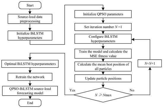
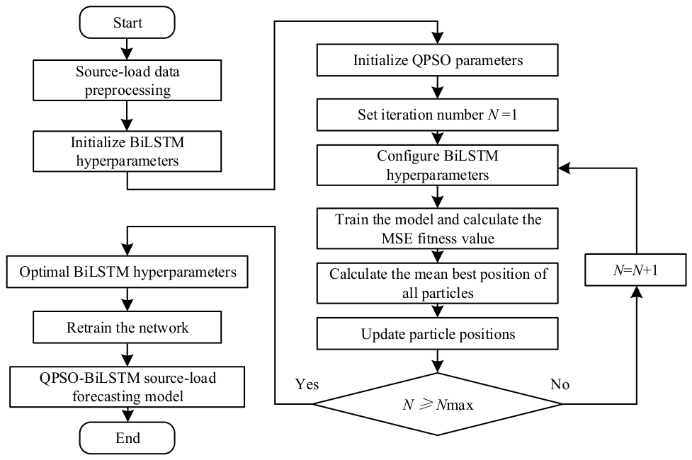
The proposed QPSO-BiLSTM forecasting procedure is shown in Figure 3. The main steps are described below.

Figure 3. Flowchart of the QPSO-BiLSTM forecasting model.

Step 1: Data preprocessing and dataset construction. The raw load and PV power time series are first processed using the outlier detection and missing value repair methods described in Section 2.1. After preprocessing, a supervised learning dataset is constructed using a sliding time-window method. Historical load or PV power values and corresponding meteorological features are used as model inputs, and the future load or PV power values are used as outputs. The training set and test set are then formed, and both input features and output targets are normalized.

Step 2: Hyperparameter search space definition and QPSO initialization. The search space of BiLSTM hyperparameters is defined, including the number of hidden units, the maximum number of training epochs, and the learning rate. Then, the QPSO population is initialized. Each particle position represents a specific hyperparameter combination of the BiLSTM model. The population size and maximum number of QPSO iterations are also specified.

Step 3: Adaptive hyperparameter optimization using QPSO. For each particle, its position is decoded into a set of BiLSTM hyperparameters. The BiLSTM model is trained on the training set using this hyperparameter configuration, and the mean squared error (MSE) on the training set is used as the fitness value. The personal best position, global best position, mean best position, and particle positions are updated iteratively according to the QPSO update equations. The optimization process continues until the maximum number of iterations is reached or the convergence condition is satisfied.

Step 4: Model training with optimal hyperparameters. After QPSO, the optimal hyperparameter combination is obtained. The BiLSTM forecasting model is then reconstructed and trained using the optimized number of hidden units, maximum training epochs, and learning rate.

Step 5: Forecasting and result output. The trained QPSO-BiLSTM model is applied to the test set to obtain short-term load and PV power forecasting results. The predicted values are transformed back to the original scale through inverse normalization. The forecasting performance is then evaluated in the case study using multiple error indicators.

Within Figure 3, N and N_max denote the current and maximum QPSO iteration numbers used in the flowchart, respectively.

3. Experimental Setup and Case Study

To verify the effectiveness of the proposed QPSO-BiLSTM model, a case study was conducted using measured load and photovoltaic (PV) power data. The experimental design includes dataset description, input and output settings, evaluation metrics, and comparison models. The proposed model was evaluated in two forecasting tasks: short-term load forecasting and short-term PV power forecasting.

3.1. Dataset Description and Experimental Environment

The dataset used in this study consists of measured load demand and PV power output data from a regional power grid in China. The input variables include maximum temperature, average temperature, minimum temperature, humidity, load active power, and PV active power. The data were collected at a sampling interval of 15 min, meaning that each day contains 96 sampling points.

A total of 92 days of data were used in the experiments. The first 85 days constituted the training-data period, while Days 86–92 served as the seven testing target days. The resulting training samples were used to optimize and train the forecasting models, while the seven testing samples were used to evaluate their generalization performance. Both load forecasting and PV power forecasting were carried out under the same data division strategy to ensure consistency in model comparison.

To avoid information leakage, all data-dependent preprocessing and normalization parameters were determined using the training-data period and were subsequently applied to the test period.

The current validation therefore reflects the forecasting performance of the proposed model for the investigated region, time period, and operating conditions; its generalization under substantial distribution shifts, such as seasonal transitions, extreme weather, or abrupt load growth, requires further evaluation.

The forecasting model was implemented in MATLAB R2024b and executed using CPU-based computation on a 64-bit Windows platform equipped with an Intel 64-bit processor with 24 logical CPUs and approximately 32 GB of physical memory. Before model training, the raw data were processed using the data preprocessing method described in Section 2.1, including outlier detection and missing value repair. After preprocessing, the data were normalized to reduce the influence of different variable scales and improve model training stability.

3.2. Day-Ahead Multi-Step Input and Output Settings

The forecasting task in this study is formulated as a day-ahead multi-step prediction problem. Since the sampling interval is 15 min, the model outputs 96 predicted values for the next day.

The first 85 days define the training-data period, while Days 86–92 serve as the seven testing target days. The previous-day 96-point power sequence is used as part of the input for each day-ahead forecasting sample. Accordingly, the 92 consecutive days yield 91 supervised forecasting samples, comprising 84 training samples with Days 2–85 as the target days and seven testing samples with Days 86–92 as the target days.

For each forecasting sample, the model input consists of three parts: the meteorological features of the previous day, the 96 time-step power sequence of the previous day, and the meteorological features of the forecasting day. The model output is the 96 time-step power sequence of the forecasting day. For the load forecasting task, the output is the load power sequence of the next day. For the PV power forecasting task, the output is the PV power sequence of the next day.

The input and output settings are summarized in Table 1.

Table 1. Input and output settings of the forecasting model.

Item	Description
Sampling interval	15 min
Number of sampling points per day	96
Training-data period	First 85 days
Testing target days	Last 7 days (Days 86–92)
Input features	Previous-day meteorological features, previous-day 96-point power sequence, and forecasting-day meteorological features
Output target for load forecasting	Forecasting-day 96-point load power sequence
Output target for PV forecasting	Forecasting-day 96-point PV power sequence

3.3. Evaluation Metrics for Forecasting Performance

To evaluate the forecasting performance of different models, four commonly used metrics were adopted: root mean square error (RMSE), mean absolute error (MAE), mean absolute percentage error (MAPE), and coefficient of determination (R²). RMSE and MAE reflect the absolute prediction error, MAPE measures the relative forecasting error, and R² reflects the goodness of fit between predicted and actual values. Lower RMSE, MAE, and MAPE values indicate better forecasting accuracy, while a higher R² value indicates better model fitting performance.

The RMSE is defined as

$$\mathit{RMSE}=\sqrt{{\displaystyle \frac{1}{n}}{\displaystyle \sum _{i=1}^n{(y_i-{\widehat{y}}_i)}^2}}$$

(30)

The MAE is defined as

$$\mathit{MAE}={\displaystyle \frac{1}{n}}{\displaystyle \sum _{i=1}^n\left|y_i-{\widehat{y}}_i\right|}$$

(31)

The MAPE is defined as

$$\mathit{MAPE}={\displaystyle \frac{1}{n}}{\displaystyle \sum _{i=1}^n\left|\frac{y_i-{\widehat{y}}_i}{y_i}\right|\times 100\%}$$

(32)

The coefficient of determination (R²) is defined as

$$R^2=1-{\displaystyle \frac{{\displaystyle \sum _{i=1}^n{(y_i-{\widehat{y}}_i)}^2}}{{\displaystyle \sum _{i=1}^n{(y_i-\overline{y})}^2}}}$$

(33)

where i is the sample index, y_i is the actual value, ${\widehat{y}}_i$ is the predicted value, $\overline{y}$ is the average of the actual values, and n is the number of samples. For PV forecasting, MAPE was calculated only for samples with nonzero actual PV power because the percentage error is undefined when the actual value is zero. Accordingly, nighttime samples with zero actual PV output were excluded from the MAPE calculation.

3.4. Baseline Models and Comparison Settings

To verify the effectiveness of the proposed QPSO-BiLSTM model, three comparison models were selected: LSTM, BiLSTM, and PSO-BiLSTM. These models were used as benchmarks for both load forecasting and PV power forecasting. The comparison models are described as follows:

• The LSTM model is used as the basic recurrent neural network model. It captures temporal dependencies in the input sequence through gate structures, but it only processes information in a single temporal direction.
• The BiLSTM model is used to evaluate the effect of bidirectional temporal feature extraction. Compared with LSTM, BiLSTM can use both forward and backward temporal information in the input sequence.
• The PSO-BiLSTM model uses particle swarm optimization to optimize the key hyperparameters of BiLSTM, including the number of hidden units, the maximum number of training epochs, and the learning rate. This model is used to evaluate the effect of conventional swarm intelligence optimization on BiLSTM forecasting performance.
• The QPSO-BiLSTM model is the proposed model in this study. It uses QPSO to optimize the BiLSTM hyperparameters. Compared with standard PSO, QPSO introduces quantum behavior into the particle position update process, which is intended to enhance exploration capability and potentially alleviate premature convergence during hyperparameter optimization.

The comparison model settings are summarized in Table 2.

Table 2. Comparison of forecasting models.

Model	Description	Purpose
LSTM	Unidirectional long short-term memory network	Baseline time-series forecasting model
BiLSTM	Bidirectional long short-term memory network	Evaluates the effect of bidirectional temporal feature extraction
PSO-BiLSTM	BiLSTM optimized by particle swarm optimization	Evaluates the effect of conventional swarm optimization
QPSO-BiLSTM	BiLSTM optimized by quantum particle swarm optimization	Proposed model

For the baseline LSTM and BiLSTM models, the hyperparameters were predefined and kept fixed throughout the experiments. Specifically, both baseline models employed two recurrent layers with 200 hidden units in each layer, a maximum of 50 training epochs, an initial learning rate of 0.005, and a mini-batch size of 16. The Adam optimizer was used for network training [46]. The same fixed hyperparameter settings were adopted for both LSTM and BiLSTM to provide a consistent baseline for evaluating the effect of bidirectional temporal feature extraction. In contrast, for PSO-BiLSTM and QPSO-BiLSTM, the numbers of hidden units, the maximum number of training epochs, and the learning rate were automatically determined by the corresponding optimization algorithms within the predefined search spaces. All models were trained and tested using the same dataset division, input features, output targets, and evaluation metrics. This ensures that the performance differences among the models are mainly caused by model structure and hyperparameter optimization strategy rather than differences in data setting.

For PSO/QPSO-based hyperparameter optimization, the population size was set to 6 particles and the maximum number of iterations was set to 20. For QPSO, the contraction–expansion coefficient was varied linearly during the optimization process, as defined in Section 2.3. The random coefficients used in the local-attractor construction and quantum position update were independently sampled from a uniform distribution over [0,1]. Since the six particles in the initial population were also individually evaluated before the iterative optimization process, each forecasting task required a total of 6 × (1 + 20) = 126 candidate BiLSTM model evaluations during the hyperparameter search. After the optimal hyperparameter combination was obtained, the final BiLSTM model was retrained using the optimized parameters. Thus, each PSO-BiLSTM or QPSO-BiLSTM forecasting task involved 126 candidate-model evaluations during hyperparameter optimization and one additional training run for the final forecasting model.

4. Forecasting Results and Performance Discussion

This section presents the experimental results of the proposed QPSO-BiLSTM model. First, the effectiveness of the data preprocessing method is analyzed using load and PV data. Then, the forecasting performance of different models is compared in the load forecasting task and the PV power forecasting task. The results are evaluated in terms of prediction accuracy, optimized hyperparameters, convergence behavior, forecasting curves, random-seed-controlled component-wise ablation, and robustness validation.

4.1. Preprocessing Results for Abnormal and Missing Data

To verify the effectiveness of the proposed data preprocessing method, outlier detection and missing value repair experiments were performed on both load data and PV power data. The problematic data in the raw dataset include spike anomalies, drop anomalies, negative anomalies, flat anomalies, and original missing values. After detection, the identified abnormal points were set as missing values and merged with the original missing values, after which all missing entries were repaired using PCHIP interpolation.

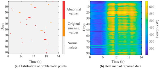
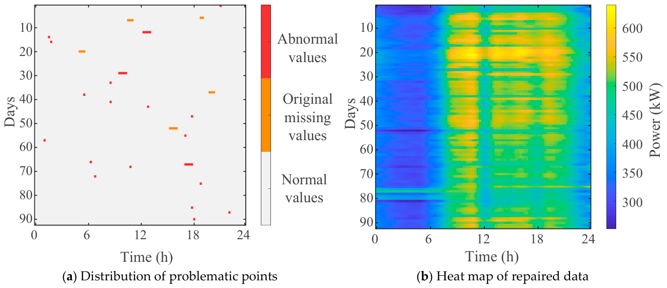
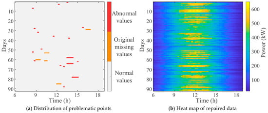
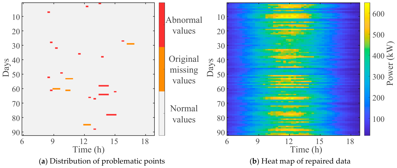
The distribution of problematic points and the global repair results for the load data are shown in Figure 4. Figure 4a shows the overall distribution of abnormal and originally missing points in the load data across different days and intra-day time periods. The problematic points are sparsely distributed without an evident concentration within a specific time period, indicating no clear recurring intra-day pattern. Figure 4b provides a global day-time view of the repaired load data. After preprocessing, the load data retain a continuous and regular intra-day variation pattern, with a coherent day-time structure and no evident artificial discontinuities introduced by the repair process. Therefore, Figure 4 is used not only to visualize the locations of problematic points but also to qualitatively assess whether the proposed preprocessing method preserves the overall temporal structure and physical consistency of the load data.

Figure 4. Preprocessing results for the load data.

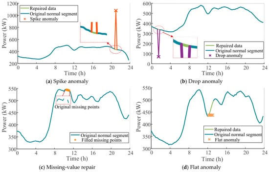
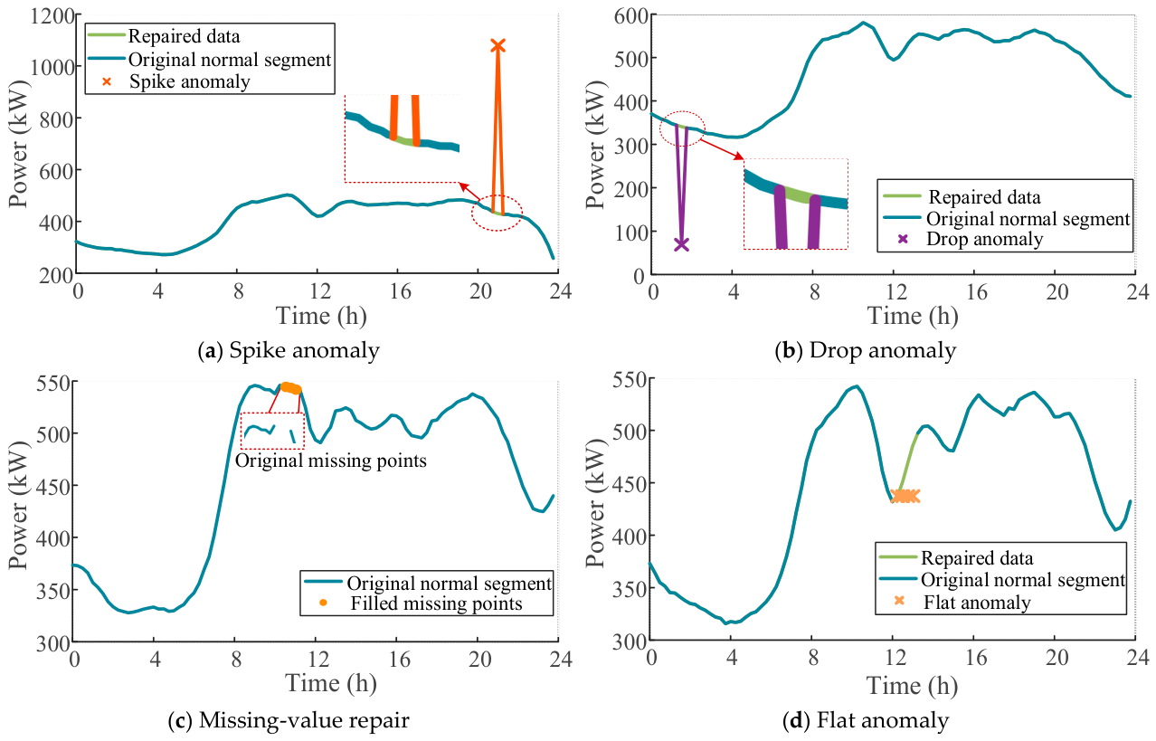
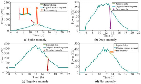
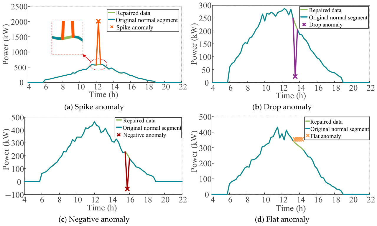
The detection and repair results of typical load anomalies are shown in Figure 5. For the spike anomaly, drop anomaly, original missing values, and flat anomaly shown in Figure 5, the repaired values are smoothly connected with the original normal segments. These examples qualitatively illustrate the local repair behavior of the proposed preprocessing method for representative abnormal load data.

Figure 5. Representative detection and repair results for load data.

The distribution of problematic points and the global repair results for the PV power data are shown in Figure 6. Compared with load data, PV power has more obvious physical characteristics: it remains zero at night and fluctuates significantly during the daytime. The proposed method considers this feature by using a cross-day same-time-slot detection strategy for PV data, which avoids misidentifying normal nighttime zero values as abnormal points.

Figure 6. Preprocessing results for the PV power data.

Figure 6a shows the distribution of abnormal and originally missing points in the PV data during the effective daytime generation period. The problematic points are sparsely distributed across different days and time slots within this period. Figure 6b presents the repaired PV data in the day-time domain. After preprocessing, the PV data preserve the typical daily generation pattern, with power gradually increasing in the morning, remaining relatively high around midday, and decreasing toward the evening. The coherent day-time structure and the absence of evident discontinuities indicate that the repair process maintains the temporal continuity and physical characteristics of PV generation.

Representative local repair results for typical PV power anomalies are further presented in Figure 7. The repaired curves are smoothly connected with the original normal segments, and the overall PV output trend remains consistent with the physical characteristics of PV generation. These examples qualitatively illustrate the local repair behavior of the proposed preprocessing method for representative abnormal PV power data.

Figure 7. Representative detection and repair results for PV power data.

To provide quantitative evidence beyond the visual examples, 20 paired semi-synthetic controlled-corruption experiments were further conducted on the measured load and PV datasets. Known anomalies and missing values were introduced into screened normal observations, so that the ground-truth anomaly locations and reference values were available for quantitative evaluation. The proposed detection method was compared with single-σ thresholding and the interquartile range (IQR) method under identical corrupted samples. Here, TP, FP, and FN denote the numbers of true positives, false positives, and false negatives, respectively. The results are shown in Table 3.

Table 3. Quantitative comparison of different anomaly-detection methods over 20 controlled-corruption experiments.

Dataset	Method	TP	FP	FN	Precision	Recall	F1-Score
Load	Proposed detector	238	0	0	1.0000	1.0000	1.0000
Load	Single-σ	238	0	0	1.0000	1.0000	1.0000
Load	IQR	237	15	1	0.9405	0.9958	0.9673
PV	Proposed detector	237	0	1	1.0000	0.9958	0.9979
PV	Single-σ	234	0	4	1.0000	0.9832	0.9915
PV	IQR	237	0	1	1.0000	0.9958	0.9979

As shown in Table 3, the proposed detector achieved F1-scores of 1.0000 and 0.9979 for the load and PV data, respectively, demonstrating consistently high detection performance across the two datasets with different physical characteristics.

To independently evaluate the repair performance, PCHIP, linear interpolation, and cubic spline interpolation were further compared using the same known abnormal/missing locations, thereby eliminating the influence of detection errors. The original measured values were used as references, and the results are reported as mean ± standard deviation (SD), together with the corresponding p-values for comparison with PCHIP, in Table 4.

Table 4. Comparison of reconstruction errors for different interpolation methods over 20 paired experiments.

Dataset	Interpolation Method	RMSE (kW), Mean ± SD	MAE (kW), Mean ± SD	RMSE p-Value vs. PCHIP	MAE p-Value vs. PCHIP
Load	PCHIP	12.0088 ± 7.0650	7.8430 ± 4.3732	-	-
Load	Linear interpolation	13.7025 ± 7.0015	9.4659 ± 4.4921	3.62 × 10−5	3.81 × 10−6
Load	Cubic spline interpolation	11.4602 ± 7.5389	7.4300 ± 4.4553	0.4980	0.3488
PV	PCHIP	28.0372 ± 7.6473	21.0522 ± 5.6000	-	-
PV	Linear interpolation	26.1036 ± 7.4186	19.4396 ± 5.2588	0.0759	0.0328
PV	Cubic spline interpolation	46.1239 ± 18.6189	34.5331 ± 12.9727	1.91 × 10−5	5.72 × 10−6

For the load data, PCHIP significantly reduced the RMSE and MAE compared with linear interpolation and achieved performance statistically comparable to cubic spline interpolation. For the PV data, PCHIP significantly outperformed cubic spline interpolation, although linear interpolation yielded slightly lower point-wise errors. Overall, PCHIP did not outperform every baseline under every metric, but it exhibited competitive and stable reconstruction performance across both load and PV data. Together with the detection results in Table 3, these results demonstrate that the adopted preprocessing scheme provides robust overall performance across data with different temporal and physical characteristics.

In summary, the proposed data preprocessing method can effectively identify and repair spike anomalies, drop anomalies, negative anomalies, flat anomalies, and original missing values. The repaired data provide a reliable data basis for subsequent load and PV power forecasting.

4.2. Load Forecasting Accuracy and Convergence Analysis

To verify the performance of the proposed QPSO-BiLSTM model in the load forecasting task, LSTM, BiLSTM, PSO-BiLSTM, and QPSO-BiLSTM were compared on the load test set. The forecasting error metrics are shown in Table 5, and the optimized hyperparameters obtained by PSO and QPSO are shown in Table 6.

Table 5. Error metrics of different models for load forecasting.

Model	RMSE (kW)	MAE (kW)	MAPE (%)	R2
LSTM	16.2908	13.2896	2.9434	0.9443
BiLSTM	14.7512	11.5048	2.5843	0.9538
PSO-BiLSTM	13.6912	10.8474	2.4197	0.9606
QPSO-BiLSTM	12.5709	9.7745	2.1616	0.9663

Table 6. Hyperparameters of BiLSTM optimized by PSO and QPSO for load forecasting.

Parameter	PSO-BiLSTM	QPSO-BiLSTM
Number of units in hidden layer 1	175	169
Number of units in hidden layer 2	160	166
Maximum training epochs	41	28
Learning rate	0.00416	0.00449

As shown in Table 5, the forecasting results obtained from the measured grid data exhibit progressively lower errors from LSTM to QPSO-BiLSTM. Compared with LSTM, BiLSTM reduces RMSE, MAE, and MAPE, indicating the potential benefit of bidirectional temporal feature extraction for load forecasting. Hyperparameter optimization further reduces the prediction errors, and QPSO-BiLSTM obtains the lowest RMSE, MAE, and MAPE and the highest R² among the four models in this comparison, with values of 12.5709 kW, 9.7745 kW, 2.1616%, and 0.9663, respectively. Compared with the baseline LSTM model, QPSO-BiLSTM reduces all three error metrics by more than 20%. The robustness and statistical significance of these performance differences are further examined through random-seed-controlled validation in Section 4.4.

Table 6 shows the optimal hyperparameters obtained by PSO and QPSO. The results indicate that different optimization algorithms search for different parameter combinations. QPSO obtains a relatively balanced hidden-layer structure and a suitable learning rate, which helps the model achieve better forecasting performance with fewer training epochs.

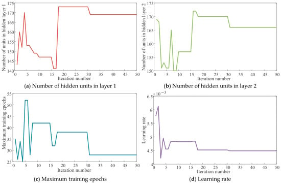
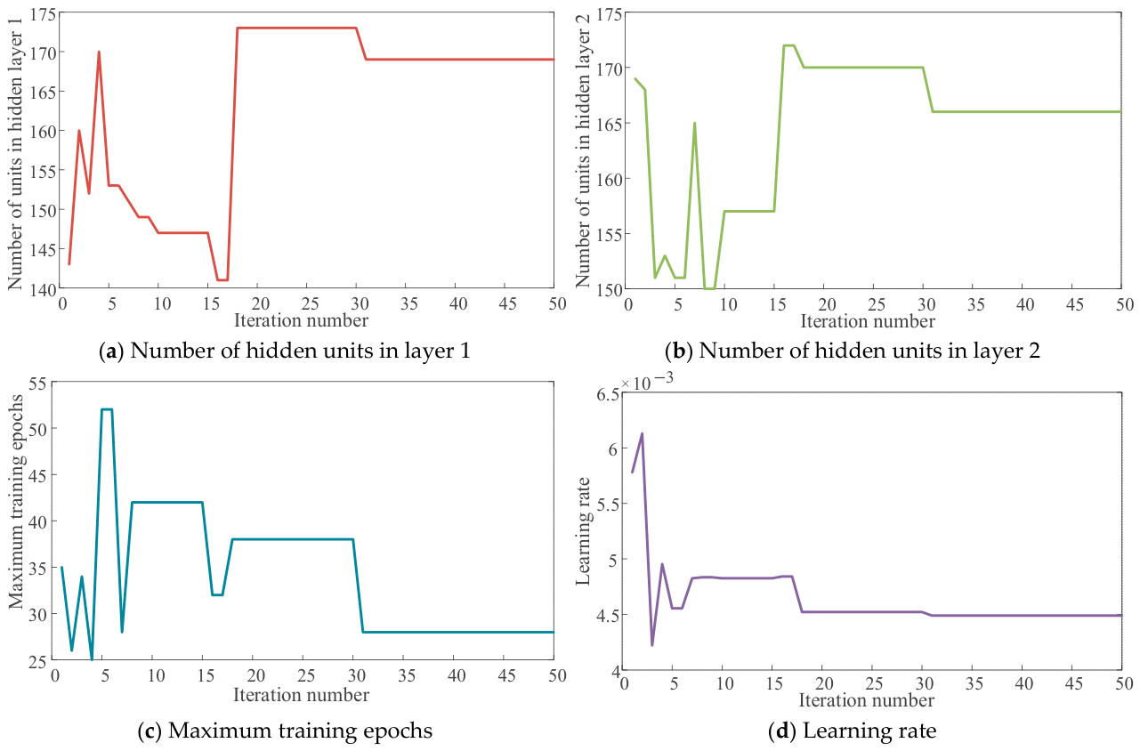
The evolution of BiLSTM hyperparameters during the QPSO process is shown in Figure 8. At the early stage of optimization, the hyperparameters fluctuate in a wide range, indicating that the particles perform global exploration in the search space. As the iteration proceeds, the fluctuation range gradually narrows, and the parameters finally converge to stable values. This process reflects the transition from global exploration to local exploitation.

Figure 8. Evolution of the BiLSTM hyperparameters during QPSO for load forecasting.

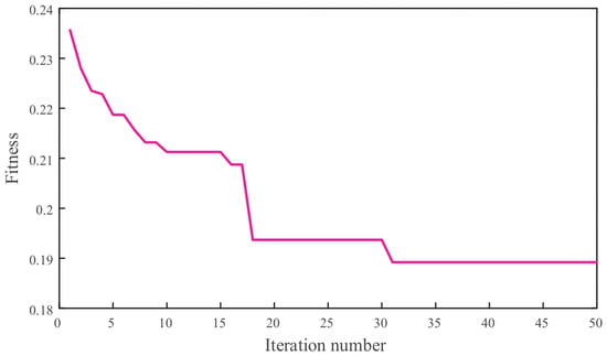
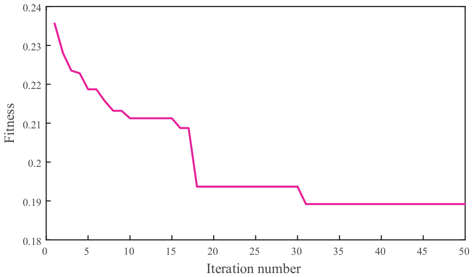
The QPSO fitness convergence curve for load forecasting is shown in Figure 9. The fitness value decreases rapidly during the early iterations and then gradually stabilizes, illustrating the convergence behavior of QPSO under the adopted optimization settings.

Figure 9. Fitness convergence curve of QPSO for load forecasting.

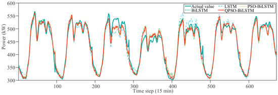
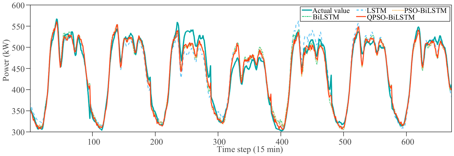
The overall forecasting curves of the seven-day load test set are shown in Figure 10. All four models can generally follow the overall trend of the actual load curve, especially during relatively stable periods. However, obvious differences appear at peak–valley transition points and periods with large fluctuations. LSTM and BiLSTM show certain lag or deviation at some extreme points, while PSO-BiLSTM and QPSO-BiLSTM fit the actual curve more closely. The QPSO-BiLSTM curve generally follows the actual load profile more closely during the major fluctuation periods, which is consistent with the lower forecasting errors reported in Table 5.

Figure 10. Comparison of load forecasting results of different models on the seven-day test set.

4.3. PV Power Forecasting Accuracy and Performance Analysis

To further evaluate the forecasting performance of the proposed model for a power series with stronger intermittency and variability, the four models were also compared on the PV power forecasting task. The forecasting error metrics are shown in Table 7, and the optimized hyperparameters obtained by PSO and QPSO are shown in Table 8.

Table 7. Error metrics of different models for PV power forecasting.

Model	RMSE (kW)	MAE (kW)	MAPE (%)	R2
LSTM	67.7222	41.5265	27.9792	0.8379
BiLSTM	24.4043	12.9557	8.8357	0.9787
PSO-BiLSTM	23.5882	12.9355	8.8587	0.9781
QPSO-BiLSTM	21.8955	11.2943	7.5687	0.9828

Table 8. Hyperparameters of BiLSTM optimized by PSO and QPSO for PV power forecasting.

Parameter	PSO-BiLSTM	QPSO-BiLSTM
Number of units in hidden layer 1	186	196
Number of units in hidden layer 2	148	157
Maximum training epochs	10	82
Learning rate	0.00924	0.00443

As shown in Table 7, the four models exhibit clear differences in the primary forecasting evaluation on measured grid data. LSTM produces the largest errors, whereas BiLSTM substantially reduces RMSE, MAE, and MAPE. QPSO-BiLSTM obtains the lowest RMSE, MAE, and MAPE and the highest R², with values of 21.8955 kW, 11.2943 kW, 7.5687%, and 0.9828, respectively. Compared with BiLSTM, QPSO-BiLSTM reduces RMSE and MAE by approximately 10.3% and 12.8%, respectively. These results demonstrate favorable forecasting performance of QPSO-BiLSTM for the considered PV test period, while the robustness of the differences among architectures and optimization strategies is further evaluated in Section 4.4.

It is worth noting that the MAPE of PSO-BiLSTM is slightly higher than that of BiLSTM, although its RMSE and MAE are lower. This suggests that, in the primary forecasting evaluation on measured grid data, the two optimization strategies converged to different regions of the hyperparameter space. In this case, QPSO produced a parameter configuration associated with lower overall forecasting errors for the PV forecasting task.

As shown in Table 8, PSO and QPSO obtain different optimal hyperparameter combinations for the PV power forecasting task. This difference is consistent with the discussion in Section 2.3 that standard PSO may suffer from premature convergence and limited search capability, whereas QPSO alleviates these limitations through its quantum-behavior-based position update mechanism. Consequently, QPSO identifies a more favorable combination of training epochs and learning rate, which allows more adequate training with more stable parameter updates, providing a better balance between training depth and update stability for the strongly fluctuating and intermittent PV power series.

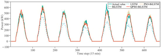
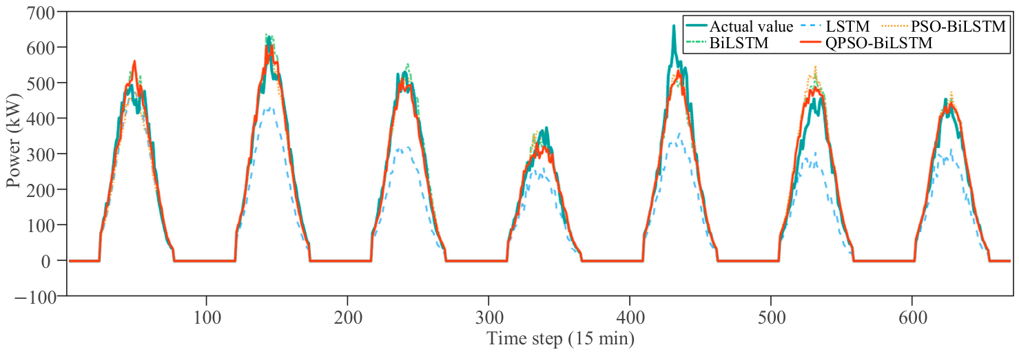
The overall forecasting curves of the PV power test set are shown in Figure 11. All four models can capture the general daily variation trend of PV output and accurately predict the zero-output period at night. However, during the daytime peak period and rapid power-drop periods, the LSTM prediction curve deviates significantly from the actual curve, and the peak power is clearly underestimated. BiLSTM and the two optimized models show better tracking performance in the peak region. Among them, QPSO-BiLSTM achieves the closest fit to the actual PV output curve and maintains high accuracy during rapid rising and falling periods. These curves illustrate the ability of QPSO-BiLSTM to track the overall PV generation profile and rapid power variations during the considered test period.

Figure 11. Comparison of PV power forecasting results of different models on the seven-day test set.

The computational cost of QPSO was further evaluated to assess the practical applicability of the proposed method. For the load forecasting task, the QPSO hyperparameter search required 2660.76 s (approximately 44.35 min), while retraining the final BiLSTM model using the optimized hyperparameters required 21.68 s. Prediction over the complete test set required only 0.0163 s, resulting in a total computational time of 2682.46 s (approximately 44.71 min). For the PV power forecasting task, the corresponding QPSO search, final model training, and prediction times were 2417.47 s (approximately 40.29 min), 19.75 s, and 0.0162 s, respectively, resulting in a total computational time of 2437.24 s (approximately 40.62 min). The total computational time for the two forecasting tasks was therefore approximately 85.33 min (1.42 h).

Although QPSO introduces additional computational costs because multiple candidate BiLSTM models must be repeatedly trained during hyperparameter optimization, this computational burden is primarily concentrated in the offline optimization stage. Once the optimal hyperparameters are obtained, the final model requires only approximately 20 s for training and approximately 0.016 s for prediction over the complete test set.

In the primary forecasting evaluation on measured grid data reported in Section 4.2 and Section 4.3, QPSO-BiLSTM reduced RMSE, MAE, and MAPE relative to the conventional BiLSTM model by approximately 14.8%, 15.0%, and 16.4%, respectively, for load forecasting, and by approximately 10.3%, 12.8%, and 14.3%, respectively, for PV forecasting. The additional computational burden is concentrated in the offline hyperparameter-search stage, whereas prediction over the complete test set requires only approximately 0.016 s. Therefore, the proposed optimization framework remains practical for the day-ahead forecasting scenario considered in this study.

Overall, the proposed framework achieves favorable forecasting performance for both load and PV power. The contributions of its individual components and the robustness of the observed performance differences are further quantified through the random-seed-controlled ablation and robustness validation in Section 4.4.

4.4. Random-Seed-Controlled Ablation and Robustness Analysis

To further quantify the contributions of data preprocessing, the BiLSTM architecture, and QPSO-based hyperparameter optimization, random-seed-controlled ablation and robustness experiments were conducted under stochastic training and optimization. All experiments adopted the same data partition and evaluation protocol. Ten paired runs were performed using random seeds 1001–1010, and the same random seed was used for each corresponding paired comparison. The results are reported as mean ± standard deviation (SD), and the paired Wilcoxon signed-rank test was used to assess statistical significance [47]. To ensure a consistent reference across different ablation configurations, all metrics in this section were calculated against the screened original observations and are used primarily to evaluate the relative contributions of the individual components and their robustness across random seeds.

Four comparison settings were considered. The minimal-preprocessing model only performed the necessary filling of NaN values and was used to assess the overall contribution of anomaly detection and repair. The simple-preprocessing model adopted single-σ detection and linear interpolation to provide a conventional preprocessing baseline. The matched-hyperparameter LSTM used the same QPSO-selected hyperparameters as the complete model, with BiLSTM replaced by a unidirectional LSTM, thereby isolating the contribution of bidirectional temporal feature extraction. Finally, PSO-BiLSTM and QPSO-BiLSTM used the same search space, population size, and maximum number of iterations to compare the two hyperparameter optimization strategies. The results of the random-seed-controlled validation are summarized in Table 9.

Table 9. Forecasting performance of different ablation configurations across 10 paired runs with controlled random seeds (mean ± SD).

Dataset	Experimental Configuration	RMSE (kW)	MAE (kW)	MAPE (%)	R2
Load	Complete QPSO-BiLSTM	29.4092 ± 2.0422	23.3676 ± 1.7508	5.3852 ± 0.5047	0.8748 ± 0.0171
Load	Minimal preprocessing + BiLSTM	33.4785 ± 2.9910	26.6672 ± 2.6380	6.1513 ± 0.8807	0.8374 ± 0.0300
Load	Simple preprocessing + BiLSTM	29.8389 ± 2.8465	24.1558 ± 2.6451	5.7196 ± 0.7207	0.8707 ± 0.0253
Load	Matched-hyperparameter LSTM	30.6564 ± 3.5724	24.7117 ± 2.9565	5.7897 ± 0.8300	0.8629 ± 0.0320
Load	PSO-BiLSTM	33.5276 ± 5.4727	27.2369 ± 4.1260	6.4424 ± 0.8861	0.8342 ± 0.0545
PV	Complete QPSO-BiLSTM	81.9398 ± 11.9910	49.2109 ± 9.3131	27.6691 ± 5.8072	0.7989 ± 0.0619
PV	Minimal preprocessing + BiLSTM	81.5079 ± 9.9536	49.0461 ± 6.7240	26.8484 ± 3.4837	0.8021 ± 0.0515
PV	Simple preprocessing + BiLSTM	85.3908 ± 12.0289	51.2387 ± 8.6874	29.6447 ± 5.9967	0.7819 ± 0.0619
PV	Matched-hyperparameter LSTM	77.8372 ± 11.4251	48.2079 ± 7.5330	26.7146 ± 4.1900	0.8185 ± 0.0498
PV	PSO-BiLSTM	76.1253 ± 12.9757	46.2626 ± 8.3661	25.1954 ± 3.9894	0.8252 ± 0.0595

The preprocessing module provided a clear contribution to load forecasting. Compared with the minimal-preprocessing baseline, the complete preprocessing scheme reduced RMSE, MAE, and MAPE by 12.15%, 12.37%, and 12.45%, respectively, while increasing R² from 0.8374 to 0.8748. Compared with the simple-preprocessing baseline based on single-σ detection and linear interpolation, the complete scheme further reduced RMSE, MAE, and MAPE by 1.44%, 3.26%, and 5.85%, respectively, for the load task, and by 4.04%, 3.96%, and 6.66%, respectively, for the PV task. These results indicate that the characteristic-aware anomaly detection and PCHIP-based repair provide favorable overall forecasting performance across both types of power-series data, with the strongest improvement observed when abnormal load data are explicitly detected and repaired.

The matched-hyperparameter architecture ablation further shows that BiLSTM improves the mean forecasting performance for the load task. Relative to the matched LSTM, BiLSTM reduced RMSE, MAE, and MAPE by 4.07%, 5.44%, and 6.99%, respectively, and also exhibited smaller standard deviations across the main error metrics. This result indicates that bidirectional temporal modeling contributes positively to the representation of load variation patterns. For PV forecasting, the average differences between the two architectures were smaller and did not form a consistent statistical distinction across the 10 paired runs with controlled random seeds.

The contribution of QPSO was most evident in the load forecasting task. Compared with PSO-BiLSTM, QPSO-BiLSTM reduced RMSE, MAE, and MAPE by 12.28%, 14.21%, and 16.41%, respectively, while increasing R² from 0.8342 to 0.8748. The standard deviations of QPSO-BiLSTM were also substantially smaller than those of PSO-BiLSTM, indicating that QPSO improved both the mean forecasting accuracy and stability across random seeds. For PV forecasting, the mean differences between PSO and QPSO were not statistically significant. The stronger intra-day and inter-day variability of PV power, together with the absence of direct irradiance- and cloud-related predictors in the current input set, increases the influence of exogenous variability on the forecasting results.

The statistical significance of the paired comparisons is summarized in Table 10, where p denotes the p-value obtained from the paired Wilcoxon signed-rank test.

Table 10. Paired Wilcoxon signed-rank test results for the ablation comparisons.

Dataset	Comparison	RMSE p	MAE p	MAPE p	R2 p
Load	Complete vs. minimal preprocessing	0.0020	0.0195	0.0488	0.0020
Load	Complete vs. simple preprocessing	0.9219	0.6250	0.0840	1.0000
Load	BiLSTM vs. matched-hyperparameter LSTM	0.5566	0.4316	0.2754	0.5566
Load	QPSO-BiLSTM vs. PSO-BiLSTM	0.0273	0.0059	0.0020	0.0195
PV	Complete vs. minimal preprocessing	0.8457	0.8457	0.7695	0.8457
PV	Complete vs. simple preprocessing	0.2324	0.3750	0.3750	0.2754
PV	BiLSTM vs. matched-hyperparameter LSTM	0.3750	0.6953	0.6250	0.4316
PV	QPSO-BiLSTM vs. PSO-BiLSTM	0.6953	0.6953	0.3223	0.5566

As shown in Table 10, the complete preprocessing scheme significantly outperformed the minimal-preprocessing baseline for all four load-forecasting metrics (p < 0.05). The differences between QPSO-BiLSTM and PSO-BiLSTM were also statistically significant for RMSE, MAE, MAPE, and R², confirming the robustness of the QPSO-related improvement in the load task. BiLSTM achieved lower mean errors than the matched-hyperparameter LSTM, although the differences were not statistically significant. For PV forecasting, none of the paired comparisons reached statistical significance, indicating a stronger influence of data variability on the relative performance of individual modules.

Overall, the random-seed-controlled ablation and robustness analyses further clarify the contributions of the proposed framework. The preprocessing procedure improves input quality and downstream forecasting performance, BiLSTM provides favorable mean performance and stability for load forecasting, and QPSO yields the clearest and most reproducible performance gain in the load task. Their combined effect results in a stable overall advantage for load forecasting, while the complete framework maintains competitive performance for the more variable PV forecasting task.

5. Conclusions

This paper proposed a QPSO-BiLSTM model for short-term load and photovoltaic (PV) power forecasting. To improve the quality of measured source-load data, an iterative 3σ criterion was used to detect spike, drop, negative, and flat anomalies, and PCHIP interpolation was applied to repair abnormal and missing values. Based on the preprocessed data, a BiLSTM forecasting model was constructed to capture bidirectional temporal dependencies in load and PV power series. QPSO was then introduced to optimize the key hyperparameters of BiLSTM, including the number of hidden units, maximum training epochs, and learning rate.

The main conclusions are as follows:

• The proposed data preprocessing method can effectively identify and repair abnormal and missing values in load and PV power data. By considering the different physical characteristics of load and PV power series, the method improves the quality and continuity of the input data and provides a reliable basis for subsequent model training.
• BiLSTM provides bidirectional temporal feature extraction for source-load forecasting. In the matched-hyperparameter ablation, BiLSTM achieves lower mean forecasting errors and smaller variability across random seeds than LSTM for the load task. For the more variable PV task, the two architectures show comparable performance across the 10 controlled random seeds.
• In the primary forecasting evaluation on measured grid data, QPSO-BiLSTM obtained the lowest forecasting errors among the compared models, with MAPE values of 2.1616% for load forecasting and 7.5687% for PV power forecasting. The random-seed-controlled robustness validation further confirmed statistically significant improvements of QPSO over PSO for load forecasting: RMSE, MAE, and MAPE were reduced by 12.28%, 14.21%, and 16.41%, respectively, together with lower variability across random seeds. For PV forecasting, the complete framework maintained competitive forecasting performance.

Several scientific and practical issues remain for further investigation. First, the statistical characteristics of load and PV power may vary with season, region, and operating conditions. Future work will therefore investigate adaptive modeling and robustness under distribution shifts to improve cross-scenario generalization. Second, QPSO-based hyperparameter optimization requires repeated training of candidate networks. Evaluating its computational scalability and optimization stability on larger datasets, in higher-dimensional search spaces, and in rolling model-update scenarios therefore remains an important direction for future research, together with the development of more efficient search and update strategies. Third, for PV forecasting, the current input features do not include direct meteorological drivers such as solar irradiance and cloud cover. Incorporating richer physically relevant variables may improve the representation of rapid weather-driven PV fluctuations. In addition, feature-contribution analysis and uncertainty quantification will be explored to enhance model interpretability, together with practical deployment strategies for online rolling forecasting and real-time power-system scheduling.

References

- Ochoa-Barragán, R.; Saavedra-Sánchez, L.D.; Nápoles-Rivera, F.; Ramírez-Márquez, C.; Lira-Barragán, L.F.; Ponce-Ortega, J.M. Artificial Intelligence Enabling Intelligent Solar Energy Systems: Integration and Emerging Directions. Processes 2026, 14, 1167. [Google Scholar] [CrossRef] [Scilit]
- Zhu, Q.; Li, J.; Qiao, J.; Shi, M.; Wang, C. Application and Prospect of Artificial Intelligence Technology in Renewable Energy Forecasting. Proc. CSEE 2023, 43, 3027–3047. [Google Scholar] [CrossRef]
- Xie, L.; Li, C.; Luo, Y.; Li, L. A Short-Term Photovoltaic Power Prediction Based on Multidimensional Feature Fusion of Satellite Cloud Images. Processes 2026, 14, 846. [Google Scholar] [CrossRef] [Scilit]
- Iheanetu, K.J. Solar Photovoltaic Power Forecasting: A Review. Sustainability 2022, 14, 17005. [Google Scholar] [CrossRef] [Scilit]
- Raza, M.Q.; Nadarajah, M.; Ekanayake, C. On Recent Advances in PV Output Power Forecast. Sol. Energy 2016, 136, 125–144. [Google Scholar] [CrossRef] [Scilit]
- Ji, X.; Zhao, G.; Ye, P.; Meng, X.; Yang, M.; Zhang, Y. Short-Term Photovoltaic Power Forecasting Method Based on QMD-HBiGRU. High Volt. Eng. 2024, 50, 3850–3859. [Google Scholar]
- Qin, Z.; Wei, H.; Deng, X.; Zhang, Y.; Wang, X. Photovoltaic Power Prediction Based on Multi-Source Environmental Information Fusion Using a VMD-ZOA-LSTM Hybrid Mode. Processes 2026, 14, 1166. [Google Scholar] [CrossRef] [Scilit]
- Bao, Z.; Wang, L.; Zhang, P.; Zhang, C.; Liu, H. Short-Term Load Forecasting Based on Hybrid Feature Selection and Spatio-Temporal Convolutional Attention Mechanism. Power Syst. Technol. 2025, 49, 5028–5037. [Google Scholar] [CrossRef]
- Yang, S.; Zhou, Z.; Chen, Y.; Liu, J.; Gong, Y. Short-Term Power Load Forecasting Method Considering Regional Adjacency Characteristics. Proc. CSU-EPSA 2024, 36, 130–139. [Google Scholar] [CrossRef]
- Xiao, J.-W.; Liu, P.; Fang, H.; Liu, X.-K.; Wang, Y.-W. Short-Term Residential Load Forecasting with Baseline-Refinement Profiles and Bi-Attention Mechanism. IEEE Trans. Smart Grid 2024, 15, 1052–1062. [Google Scholar] [CrossRef] [Scilit]
- Han, F.; Wang, X.; Qiao, J.; Shi, M.; Pu, T. Review on Artificial Intelligence-Based Load Forecasting Research for the New-Type Power System. Proc. CSEE 2023, 43, 8569–8591. [Google Scholar]
- Wang, H.; Lei, Z.; Zhang, X.; Zhou, B.; Peng, J. A Review of Deep Learning for Renewable Energy Forecasting. Energy Convers. Manag. 2019, 198, 111799. [Google Scholar] [CrossRef] [Scilit]
- Husein, M.; Gago, E.J.; Balfaqih, H.; Pegalajar, M.C. Towards Energy Efficiency: A Comprehensive Review of Deep Learning-Based Photovoltaic Power Forecasting Strategies. Heliyon 2024, 10, e33419. [Google Scholar] [CrossRef] [Scilit]
- Zhang, F.; Zhang, F.; Zhang, S. Power Load Forecasting in the Time Series Analysis Method Based on Lifting Wavelet. Electr. Autom. 2017, 39, 72–76. [Google Scholar]
- Shi, W.; Wu, K.; Wang, D.; Wang, D. Electric Power System Short-Term Load Forecasting Model Based on Time Series Analysis and Kalman Filter Algorithm. Tech. Autom. Appl. 2018, 37, 9–12, 23. [Google Scholar]
- Yang, G.; Zheng, H.; Zhang, H.; Jia, R. Short-Term Load Forecasting Based on Holt-Winters Exponential Smoothing and Temporal Convolutional Network. Autom. Electr. Power Syst. 2022, 46, 73–82. [Google Scholar]
- Chen, K.; Chen, K.; Wang, Q.; He, Z.; Hu, J.; He, J. Short-Term Load Forecasting with Deep Residual Networks. IEEE Trans. Smart Grid 2019, 10, 3943–3952. [Google Scholar] [CrossRef] [Scilit]
- Hochreiter, S.; Schmidhuber, J. Long Short-Term Memory. Neural Comput. 1997, 9, 1735–1780. [Google Scholar] [CrossRef] [Scilit]
- Kong, W.; Dong, Z.Y.; Jia, Y.; Hill, D.J.; Xu, Y.; Zhang, Y. Short-Term Residential Load Forecasting Based on LSTM Recurrent Neural Network. IEEE Trans. Smart Grid 2019, 10, 841–851. [Google Scholar] [CrossRef] [Scilit]
- Wang, T.; Wang, X.; Xu, Y.; Li, W. Study on LSTM Photovoltaic Output Prediction Model Considering Similar Days. Acta Energiae Solaris Sin. 2023, 44, 316–323. [Google Scholar] [CrossRef]
- Shi, J.; Wang, Y.; Zhou, Y.; Ma, Y.; Gao, J.; Wang, S.; Fu, Z. Bayesian Optimization-LSTM Modeling and Time Frequency Correlation Mapping Based Probabilistic Forecasting of Ultra-Short-Term Photovoltaic Power Outputs. IEEE Trans. Ind. Appl. 2024, 60, 2422–2430. [Google Scholar] [CrossRef] [Scilit]
- Schuster, M.; Paliwal, K.K. Bidirectional Recurrent Neural Networks. IEEE Trans. Signal Process. 1997, 45, 2673–2681. [Google Scholar] [CrossRef] [Scilit]
- Guo, Y.; Li, Y.; Qiao, X.; Zhang, Z.; Zhou, W.; Mei, Y.; Lin, J.; Zhou, Y.; Nakanishi, Y. BiLSTM Multitask Learning-Based Combined Load Forecasting Considering the Loads Coupling Relationship for Multienergy System. IEEE Trans. Smart Grid 2022, 13, 3481–3492. [Google Scholar] [CrossRef] [Scilit]
- Sun, H.; Yang, F.; Gao, Z.; Hu, S.; Wang, Z.; Liu, J. Short-Term Load Forecasting Based on Mutual Information and Bi-directional Long Short-term Memory Network Considering Fluctuation in Importance Values of Features. Autom. Electr. Power Syst. 2022, 46, 95–103. [Google Scholar] [CrossRef]
- Tang, D.; Zhu, W.; Hou, L. Ultra-Short-Term Photovoltaic Power Forecasting Based on the CNN-LSTM-XGBoost Model. Chin. J. Power Sources 2022, 46, 1048–1052. [Google Scholar] [CrossRef] [Scilit]
- Ren, J.; Wei, H.; Zou, Z.; Hou, T.; Yuan, Y.; Shen, J.; Wang, X. Ultra-Short-Term Power Load Forecasting Based on CNN-BiLSTM-Attention. Power Syst. Prot. Control 2022, 50, 108–116. [Google Scholar]
- Zhao, H.; Wu, Y.; Ma, L.; Pan, S. Spatial and Temporal Attention-Enabled Transformer Network for Multivariate Short-Term Residential Load Forecasting. IEEE Trans. Instrum. Meas. 2023, 72, 1–11. [Google Scholar] [CrossRef] [Scilit]
- Wang, J.; Wang, K.; Li, Z.; Lu, H.; Jiang, H.; Xing, Q. A Multitask Integrated Deep-Learning Probabilistic Prediction for Load Forecasting. IEEE Trans. Power Syst. 2024, 39, 1240–1250. [Google Scholar] [CrossRef] [Scilit]
- Ryu, S.; Yu, Y. Quantile-Mixer: A Novel Deep Learning Approach for Probabilistic Short-Term Load Forecasting. IEEE Trans. Smart Grid 2024, 15, 2237–2250. [Google Scholar] [CrossRef] [Scilit]
- Liu, Y.; Yu, H.; Liu, W.; Huang, M.; Li, L.; Zhang, S. Abnormal Data Identification for Distributed Photovoltaic Generation Based on DTW and a Two-Stage Quartile Method. Therm. Power Gener. 2024, 53, 34–44. [Google Scholar]
- Mumtahina, U.; Alahakoon, S.; Wolfs, P. Hyperparameter Tuning of Load-Forecasting Models Using Metaheuristic Optimization Algorithms—A Systematic Review. Mathematics 2024, 12, 3353. [Google Scholar] [CrossRef] [Scilit]
- Kennedy, J.; Eberhart, R. Particle Swarm Optimization. In Proceedings of ICNN’95—International Conference on Neural Networks, Perth, WA, Australia, 27 November–1 December 1995; IEEE: Piscataway, NJ, USA, 1995; Volume 4, pp. 1942–1948. [Google Scholar]
- Clerc, M.; Kennedy, J. The Particle Swarm-Explosion, Stability, and Convergence in a Multidimensional Complex Space. IEEE Trans. Evol. Comput. 2002, 6, 58–73. [Google Scholar] [CrossRef] [Scilit]
- Sun, J.; Fang, W.; Wu, X.; Palade, V.; Xu, W. Quantum-Behaved Particle Swarm Optimization: Analysis of Individual Particle Behavior and Parameter Selection. Evol. Comput. 2012, 20, 349–393. [Google Scholar] [CrossRef] [Scilit]
- Thipwangmek, N.; Suetrong, N.; Taparugssanagorn, A.; Tangparitkul, S.; Promsuk, N. Enhancing Short-Term Solar Photovoltaic Power Forecasting Using a Hybrid Deep Learning Approach. IEEE Access 2024, 12, 108928–108941. [Google Scholar] [CrossRef] [Scilit]
- Wang, K.; Shan, S.; Dou, W.; Wei, H.; Zhang, K. A Robust Photovoltaic Power Forecasting Method Based on Multimodal Learning Using Satellite Images and Time Series. IEEE Trans. Sustain. Energy 2025, 16, 970–980. [Google Scholar] [CrossRef] [Scilit]
- Wang, Z.; Zhang, H.; Yang, R.; Chen, Y. Improving Model Generalization for Short-Term Customer Load Forecasting With Causal Inference. IEEE Trans. Smart Grid 2025, 16, 424–436. [Google Scholar] [CrossRef] [Scilit]
- Liu, Y.; Zhang, Z.; Ma, L.; Jia, Y.; Yin, W.; Liu, Z. Short-Term Prediction of Photovoltaic Power Based on DBSCAN-SVM Data Cleaning and PSO-LSTM Model. Energy Eng. 2024, 121, 3019–3035. [Google Scholar] [CrossRef] [Scilit]
- Lin, W.; Zhang, B.; Lu, R. A Novel Hybrid Deep Learning Model for Photovoltaic Power Forecasting Based on Feature Extraction and BiLSTM. IEEJ Trans. Electr. Electron. Eng. 2024, 19, 305–317. [Google Scholar] [CrossRef] [Scilit]
- Peng, S.; Zhu, J.; Wu, T.; Yuan, C.; Cang, J.; Zhang, K.; Pecht, M. Prediction of Wind and PV Power by Fusing the Multi-Stage Feature Extraction and a PSO-BiLSTM Model. Energy 2024, 298, 131345. [Google Scholar] [CrossRef] [Scilit]
- Ma, L.; Wang, L.; Zeng, S.; Zhao, Y.; Liu, C.; Zhang, H.; Wu, Q.; Ren, H. Short-Term Household Load Forecasting Based on Attention Mechanism and CNN-ICPSO-LSTM. Energy Eng. 2024, 121, 1473–1493. [Google Scholar] [CrossRef] [Scilit]
- Raju, V.A.G.; Nayak, J.; Dash, P.B.; Mishra, M. Short-Term Solar Irradiance Forecasting Model Based on Hyper-Parameter Tuned LSTM via Chaotic Particle Swarm Optimization Algorithm. Case Stud. Therm. Eng. 2025, 69, 105999. [Google Scholar] [CrossRef] [Scilit]
- Peng, L.-L.; Yun, S.; Liu, X.-Q.; Fan, G.-F. Uncertainty Quantification and Load Forecasting Based on CPO-VMD and Hybrid Deep Learning. Electr. Power Syst. Res. 2026, 252, 112444. [Google Scholar] [CrossRef] [Scilit]
- Pukelsheim, F. The Three Sigma Rule. Am. Stat. 1994, 48, 88–91. [Google Scholar] [CrossRef] [Scilit]
- Fritsch, F.N.; Carlson, R.E. Monotone Piecewise Cubic Interpolation. SIAM J. Numer. Anal. 1980, 17, 238–246. [Google Scholar] [CrossRef] [Scilit]
- Kingma, D.P.; Ba, J. Adam: A Method for Stochastic Optimization. In Proceedings of the International Conference on Learning Representations (ICLR), San Diego, CA, USA, 7–9 May 2015. [Google Scholar]
- Wilcoxon, F. Individual Comparisons by Ranking Methods. Biom. Bull. 1945, 1, 80–83. [Google Scholar] [CrossRef] [Scilit]
Disclaimer/Publisher’s Note: The statements, opinions and data contained in all publications are solely those of the individual author(s) and contributor(s) and not of MDPI and/or the editor(s). MDPI and/or the editor(s) disclaim responsibility for any injury to people or property resulting from any ideas, methods, instructions or products referred to in the content. |
© 2026 by the authors. Licensee MDPI, Basel, Switzerland. This article is an open access article distributed under the terms and conditions of the Creative Commons Attribution (CC BY) license.