


Abstract
In medium-voltage distribution systems, switch states determine how sections are grouped and supplied by feeders, defining the sectionalized operating configuration. Changes in load demand and distributed generation output can increase losses and cause voltage violations, making an existing configuration unsuitable for the new conditions. Switching corrections can redistribute power flows to reduce losses and voltage violations, but their benefits must be balanced against switching costs. Variations in loss costs also change return scales, which can impair reinforcement learning (RL) methods that use a fixed value-learning scale. To address these challenges, we propose an adaptive soft actor-critic (A-SAC) algorithm to correct sectionalized operating configurations and minimize cumulative operating cost. The dynamic adaptation mechanism adjusts the value-learning scale as operating conditions change, guiding the agent to learn lower-cost configuration correction policies while preserving the original cost objective. A masked softmax output layer excludes infeasible switching actions. Tests on a 37-bus test system under normal, high photovoltaic (PV) output, and changing source/load conditions show cost reductions of 3.2–6.2% relative to retaining the initial configuration and lower costs than other advanced RL algorithms. In the changing source/load scenario, the mean cost is 3.2% lower than that of soft actor-critic (SAC).
1. Introduction
The growing integration of distributed generation (DG) has increased the need for flexible operation of medium-voltage distribution systems [1]. Changes in load demand and DG output affect network power flows and, if not managed, can lead to increased power losses, feeder overloads, and voltage violations. Meanwhile, the development and deployment of remotely controlled switches allow sectionalized operating configurations to be adjusted to redistribute power flows and improve network operation [2]. However, load levels, load distribution, and DG output vary over time, changing the power-flow patterns within an existing configuration [3]. These changes affect feeder loading and nodal voltages, thereby altering the operating performance of that configuration. Meanwhile, limits on switching operations couple configuration decisions across time [4]. The challenge is therefore to adapt sectionalized operating configurations to changing power-flow conditions while minimizing cumulative power-loss costs, switching costs, and voltage-violation penalties.
Such configuration adjustment involves discrete switching decisions under network operating constraints. Some studies use genetic search with nearest-neighbor mapping to obtain radial configurations [5]. Other approaches combine multi-step switch exchange with bi-level scheduling to coordinate topology adjustment and network operation [6]. However, heuristic search does not generally guarantee a globally optimal configuration. In contrast, mixed-integer optimization explicitly models switching decisions and operating constraints and provides bounds on solution quality [7]. Multi-stage robust formulations further incorporate renewable uncertainty and intertemporal switching limits [4], while sensitivity-assisted integer quadratic programming improves the efficiency of individual switching decisions [8]. Despite these advances, solving large mixed-integer problems remains computationally demanding. Accordingly, supervised-learning methods predict voltage stability indices or switching variables [9,10], while other approaches learn configuration selection rules and surrogate power-flow constraints [11]. These methods reduce parts of the online computation, but still require search or optimization to obtain the final operating decisions. Furthermore, reinforcement learning (RL) treats configuration adjustment as a sequential decision problem and learns control policies that account for the effects of switching actions on subsequent operation [1,12]. Other studies combine pre-training on historical data with safe online policy updates to support reliable network operation [13]. However, differences in section loading, supply-path impedance, and DG output lead to different return scales for configuration correction. With a shared value network, equal relative prediction errors produce larger squared losses for returns with greater magnitudes [14]. This can reduce value-estimation accuracy in conditions with smaller return magnitudes and impair the resulting configuration correction decisions.
This paper addresses the influence of return-scale differences on value learning by proposing an adaptive soft actor-critic (A-SAC) algorithm for sectionalized configuration correction. The configuration correction problem is formulated as a Markov decision process (MDP) to minimize cumulative power-loss costs, switching costs, and voltage-violation penalties. The algorithm incorporates a dynamic adaptation mechanism that adjusts value learning to evolving return scales while preserving the original operating-cost objective. The proposed algorithm is evaluated on a 37-bus medium-voltage test system under varying generation and load conditions. The results demonstrate that the proposed algorithm not only adapts sectionalized operating configurations to changing generation and load conditions but also achieves lower cumulative operating costs than other RL algorithms.
The main contributions of this research are as follows:
- An MDP formulation of sectionalized configuration correction, which models sequential switching decisions under varying generation and load conditions to minimize cumulative operating costs.
- An A-SAC algorithm with a dynamic adaptation mechanism, which accommodates evolving return scales in value learning while preserving the original operating-cost objective.
- Evaluation of the proposed algorithm on a 37-bus medium-voltage test system under varying generation and load conditions, with comparisons against other RL algorithms.
2. Related Work
Network reconfiguration is widely studied for loss reduction, voltage regulation, and reliability improvement [15,16]. Some studies use switch exchange to exploit network structure [2,3], which reduces search effort but does not generally establish a global optimum. Genetic search uses radiality mapping to avoid nonradial candidates [5], although radiality alone does not establish minimum operating cost. To account for changing operating conditions, multi-step exchange is combined with bi-level scheduling [6], and multi-timescale branch reduction coordinates stochastic operation [17]. The latter extends the range of operating conditions considered; its solution quality is assessed mainly against benchmarks without a general theoretical optimality-gap guarantee. Hybrid simulated annealing–tabu search improves exploration [18], although evaluating each candidate still requires power-flow calculation. Updating the configuration as conditions change therefore involves further search and evaluation. For post-event restoration, shortest-path heuristics jointly represent electricity and communication networks [19], showing that an electrically acceptable configuration may also depend on communication availability.
To provide bounds on solution quality, mixed-integer conic formulations use tighter relaxations for stochastic reconfiguration [7]; however, the associated multi-snapshot problem remains challenging to solve. The modeled cost also depends on how demand responds to reconfiguration. Voltage-dependent load formulations account for demand changes caused by altered nodal voltages [20,21], while temperature-dependent models additionally capture changes in consumption with ambient conditions [22]. Modeling renewable output together with load voltage dependence further accounts for changes on both sides of the power balance [23]. Beyond aggregate power, phase imbalance requires phase-specific operating constraints, as incorporated in phase-balancing and unbalanced microgrid formulations [24,25]. Fixed equipment ratings can also restrict renewable utilization, motivating joint optimization of dynamic transformer ratings and reconfiguration [26]. As operating inputs change, the suitability of a previously selected configuration must be reconsidered. Multi-stage robust optimization addresses uncertainty and intertemporal switching limits [4], while mapping-based column-and-constraint generation handles decision-dependent uncertainty [27] and distributionally robust decomposition coordinates controls under uncertain photovoltaic (PV) output distributions [28]. Their coverage of uncertain operating conditions depends on the specified uncertainty representation. Moreover, endpoint feasibility does not ensure safe implementation: switching-path optimization addresses intermediate transitions [29], and protection-aware models enforce coordination and fault-isolation requirements after topology changes [30,31]. Electrical feasibility alone also does not ensure cyber-physical security, prompting observability-constrained reconfiguration [32] and attack-aware Stackelberg formulations [33]. During outages, topology selection must additionally respect storage availability and repair timing [34,35], while recovery-sequence and transition models account for how service is restored over time [36,37]. To reduce the resulting solution burden, sensitivity-based integer optimization accelerates individual switching decisions [8]. Historical-curtailment feedback guides forecast-based daily topology selection [38], and net-load clustering restricts integer-programming schedules to a smaller candidate set [39]. Although the latter reduces online computation, forecast errors can undermine candidate selection because it relies on accurate day-ahead forecasts. This dependence motivates decisions that respond to updated operating observations.
Learning-based methods reduce online computation by replacing selected calculations with learned mappings. Predicting voltage-stability indices accelerates branch-reduction searches [9], but the prediction supplies an evaluation quantity rather than a complete switching decision. Predicting selected switch states reduces the remaining mixed-integer problem [10], while learned topology-selection trees and power-flow surrogates simplify optimization [11]; both retain a solver to complete the decision. RL instead learns a policy from operating observations: graph-based soft actor-critic (SAC) coordinates network reconfiguration with voltage and reactive-power control [12], whereas transformer policies retain alternating-current (AC) optimal power flow for dispatch feasibility [1], so policy-based topology selection does not necessarily eliminate online optimization. Direct policy learning also faces a large switching action space. Power-flow-based sampling reduces the available candidates [40], thereby restricting policy selection to the retained set. Switch-contribution-based two-stage learning allocates high- and low-contribution switches to separate stages [41], reducing the learning burden while requiring coordination between stages. Coordinating devices with different response times motivates multi-timescale policies [42]; safe execution of the selected topology additionally requires sequential-switch control [43]. Safe exploration during training is a separate requirement from execution feasibility. Constrained offline pre-training and safe online updates reduce trial-and-error risks [13], while robust-environment interaction accounts for uncertainty in safe policy learning [44]. Action masking restricts inadmissible actions during constrained policy optimization [45]. Accurate estimation of the admissible actions’ returns remains a separate learning requirement. Similarly, event-driven Q-routing [46] and attention-based multi-agent learning with action masks [47] adapt restoration actions to topology changes, while return estimation remains part of the learning problem. In sectionalized configuration correction, differences in section loading, supply-path impedance, and DG output change return magnitudes. With squared-error value learning, equal relative prediction errors then produce unequal losses, which can impair estimation across operating conditions. PopArt addresses scale dependence by adaptively normalizing value targets while preserving their original-scale predictions [14,48]. For replay-based configuration correction, calibration must track changes in complete return targets as the source/load conditions, policy, and value estimates evolve. This motivates a schedule that responds to observed range changes while continuing to track target drift between events.
3. Preliminaries
3.1. System Model
Figure 1 illustrates the four-feeder, 10 kV distribution system, comprising twelve sections and five DG units connected through points of common coupling. Sectionalizing switches lie at section boundaries, while tie switches connect sections on different feeders. Under radial operation, each section has a unique supply path to the substation. Switch states determine the sections assigned to each feeder and their supply paths, together defining the sectionalized operating configuration. The equipment within each physical section remains fixed when this configuration changes.
Figure 1.
Medium-voltage distribution system schematic.
Changes in demand and DG output alter the losses associated with these supply paths. For example, DG1 may produce surplus power in A3 while B3 has high demand and low DG3 output. Closing tie switch and opening sectionalizing switch transfers A3 to feeder B while maintaining a connected radial topology. DG1 can then supply part of B3’s demand through the tie line, reducing the current and losses on feeder B’s upstream branches. The economic value of this exchange depends on the resulting loss costs, voltage penalties, and switching costs over the remaining horizon. Sectionalized configuration correction therefore determines when and how to change section assignments and supply paths to minimize cumulative operating cost under network constraints.
3.2. Problem Definition
Changes in generation and load conditions alter the energy-loss costs of the existing configuration. Correcting the configuration may reduce these costs, but requires switch operations that incur additional costs. The objective is therefore to minimize cumulative operating cost over the full horizon by balancing loss-cost savings against switching costs. A voltage-limit violation penalty is also included to account for voltage deviations. These terms form the total cost used for optimization. The operating horizon consists of T intervals, indexed by . The cost in each interval is given by
where is the total cost in interval t, is the unit energy cost, is the active power loss under the selected configuration, and is the interval duration. The product gives the loss energy. The coefficient is the cost per switch operation, and is the number of operations. The coefficient penalizes voltage-limit violations, and is the sum of voltage excursions beyond the allowed limits at the evaluated nodes, measured in per unit. The full-horizon optimization problem is
where is the configuration correction policy and denotes the expectation under that policy.
At each interval, the controller retains the current configuration or closes one switch and opens another. Retaining the configuration incurs no switching cost, whereas one exchange counts as two operations. With a fixed cost per operation, the same exchange incurs the same switching cost across generation and load conditions. Loss energy, however, varies with branch currents and supply paths. Since line losses depend on the square of current, changes in load demand and DG output can cause substantial differences in loss energy and the savings obtained from a correction. The resulting loss-cost savings may offset the switching cost under one condition but be insufficient under another. Because the resulting configuration also affects subsequent losses, this decision must account for costs over the remaining horizon.
Even with fixed cost coefficients, these variations in loss energy can change the numerical range of cumulative costs estimated during policy learning. The selected configurations must remain connected and radial, satisfy power-flow balance, and respect branch capacity limits. The controller selects configuration corrections within these constraints to minimize cumulative operating cost over the full horizon under changing generation and load conditions.
4. A-SAC Framework
4.1. Overview of the Proposed Method
The sectionalized configuration correction problem requires switching decisions that reduce operating costs while maintaining a connected, radial network. Changes in generation and load alter loss costs and hence the scale of value-learning targets. We propose an A-SAC framework to learn feasible correction policies while adapting value learning to these scale changes.
Figure 2 shows the discrete SAC backbone for configuration correction. The masked actor assigns zero probability to infeasible actions, while twin critics and their target networks support value learning. The dynamic adaptation mechanism in Section 4.4 adjusts the target scale during training and preserves the critics’ original-scale predictions. Policy improvement uses these original-scale values, retaining the operating-cost objective.
Figure 2.
Discrete SAC backbone with action masking for sectionalized configuration correction.
4.2. MDP Formulation
We formulate sectionalized configuration correction as a finite-horizon MDP:
where denotes the MDP, is the state space, is the action space, P is the state transition probability, r is the reward function, and is the discount factor.
4.2.1. State
The state at interval t is defined as
where and are the vectors of nodal active and reactive load demand, is the vector of nodal active DG output, is the configuration of all controllable switches before the decision, and t is the time index within the operating horizon. The three power vectors use the same fixed ordering of non-source nodes, with zero DG output at nodes without DG. Load demand and DG output are taken as positive. We assume that DG units operate at unity power factor. Separate load and DG inputs distinguish operating conditions with the same net injections but different load and generation profiles.
Each entry of is 1 if the corresponding switch is closed and 0 if it is open. The position of each entry corresponds to a fixed switch index. The initial configuration is given. The switch configuration and the fixed branch connections together determine the operating topology. The state dimension is
where denotes the state dimension, n is the total number of nodes, including the source node, and m is the number of controllable switches. The net injections used in power-flow calculations are
where and are the active and reactive net injection vectors, respectively, with generation injection taken as positive. Future load and DG outputs are not included in the state.
4.2.2. Action
At each interval, the controller either retains the current configuration or closes one switch and opens another. The hold action avoids switching costs when the expected operating-cost savings from an exchange do not cover its switching cost. The action is defined as
where is the action at interval t, denotes retaining the current configuration, and denotes closing switch i and opening switch j. The switch indices correspond to their positions in . An exchange requires and ; all other switch states remain unchanged. The fixed action library has entries, where is the total number of actions. Fixed branches are excluded from switching decisions.
Only a subset of switch pairs is feasible for a given configuration. In the candidate topology, closing an open switch creates a single cycle. The switch selected for opening must lie on this cycle to preserve connectivity and radiality. Candidate exchanges and the hold action are then checked by power flow under the current load and DG output; nonconvergent solutions and branch overloads are rejected. These checks define the feasible action set . Voltage deviations enter the cost as a soft penalty, so an accepted action may still produce a voltage-limit violation. Each exchange specifies the resulting steady-state configuration. The close–open notation identifies the two changed switch states; it does not prescribe the physical order or timing of their operation. An execution procedure must check the intermediate states and protection coordination before implementing the selected exchange.
4.2.3. State Transition
Let denote the joint load and DG input. The selected action updates the switch configuration, and the time index advances by one:
where F is the configuration update function, is the configuration after the action, and is the next state. The environment evaluates the current interval’s cost using and before advancing to . Load and DG output follow a joint transition model, denoted by . This model conditions their next values on and t and allows dependence between load and DG output. Under this model, switching actions do not affect their evolution. The state transition probability is therefore
for next states whose configuration and time index satisfy (8), and zero otherwise. Prescribed load and DG time series are a deterministic special case.
4.2.4. Reward
To minimize operating costs, we define the reward as the negative interval cost:
where is the reward in interval t, is the interval cost defined in (1), is the unit energy cost, is active power loss, and is the interval duration. The coefficient is the cost per switch operation, is the operation count, is the voltage-violation penalty coefficient, and is the total voltage-limit violation. Losses and voltages are evaluated under the current injections and the configuration after the action. The operation count is
where ℓ indexes the controllable switches. The count is zero for a hold action and two for an exchange. The total voltage-limit violation is
where is the set of nodes included in the voltage evaluation, is the voltage magnitude at node i in per unit, and and are its lower and upper limits. The penalty is zero when all evaluated voltages are within their limits and grows in proportion to the total voltage deviation and interval duration. Retaining the configuration avoids switching costs but still incurs energy-loss costs and any voltage-violation penalty.
We set so that future costs are not discounted. Maximizing expected cumulative reward is then equivalent to minimizing expected full-horizon cost:
where is the correction policy, denotes expectation under that policy, and T is the number of intervals in the operating horizon. The episode ends after the cost in interval T is evaluated, and the terminal value is zero. The policy thus balances switching costs against current and future operating costs. We use discrete SAC to learn this policy and introduce dynamic adaptation through value normalization to accommodate changes in cumulative-return scale. Normalization statistics are updated through event-triggered and periodic calibration. The reward retains its original cost definition, and policy updates use action values on the original cost scale.
4.3. Learning a Correction Policy with Discrete SAC
To learn a correction policy for the MDP, we use discrete SAC [49]. SAC is an off-policy actor–critic algorithm that combines expected return with an entropy bonus for exploration [50]. The actor , with parameters , determines the action probabilities. Two independent critics each provide action-value estimates through linear outputs, where is the number of actions. Their target networks provide bootstrap estimates, and the smaller of the two estimates is used to reduce overestimation. For configuration correction, this formulation must exclude infeasible exchanges, separate exploration from the final cost objective, and accommodate changes in value scale. We describe these adaptations below.
4.3.1. Feasible Action Selection
A switching decision must preserve a connected radial network and respect branch capacities. Closing a tie switch creates a cycle; opening a controllable switch on that cycle restores radiality while keeping all sections connected [51]. Opening a switch outside the cycle instead leaves the cycle intact and disconnects part of the network from the substation. Even a topologically valid exchange can overload a line if the transferred load raises its current above its rating. Feasibility therefore depends on both the current switch configuration and the load and DG output.
The actor outputs one score for each action in the fixed library. A standard softmax layer converts these scores into an action distribution:
where is the score for action a at state s, is the full action library, and b indexes its entries. Every action with a finite score receives positive probability, even if it violates the network constraints.
To exclude these actions, we construct a binary mask before action selection. First, a candidate pair must close a currently open switch i and open a currently closed, controllable switch j on the resulting cycle. We then solve power flow under the current load and DG output and reject candidates with nonconvergence or branch overloads. The mask is 1 for an exchange that passes these checks and 0 otherwise. The hold action undergoes the same power-flow and capacity checks. Voltage violations remain part of the reward penalty.
To ensure that only feasible actions receive positive probability, we use a masked softmax output layer [51]:
which sets rejected actions’ probabilities to zero and normalizes the remaining probabilities to sum to one. The layer is differentiable with respect to the actor scores, allowing policy gradients to update and learn probabilities over feasible actions. Softmax has no trainable parameters of its own: the actor learns the scores, while the constraint-based mask remains fixed during each update.
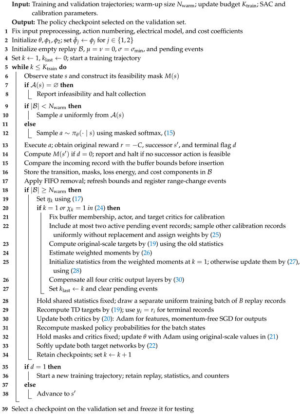
At each decision, the mask is recomputed and one action is selected from . Rejected scores are set to before softmax. Policy updates use the current-state mask, whereas value targets use the next-state mask. Before applying softmax, Algorithm 1 checks that the action set is nonempty. If it is empty, the prescribed procedure reports infeasibility within the hold-or-one-exchange control scope and stops the affected trajectory before action selection. The trajectory is recorded as incomplete rather than assigned a completed-horizon cost. A hold action is available only when it passes the same electrical checks. The zero terminal value applies only to completion of the operating horizon.
4.3.2. Exploration Schedule
A switch exchange incurs an immediate cost, while its loss savings may continue over later intervals. Before the critics learn these future savings, the policy may favor holding the configuration. To encourage exploration of alternative feasible supply paths, SAC includes an entropy bonus. The policy entropy is defined as
where H measures the dispersion of action probabilities and log is the natural logarithm. Its maximum is , where is the number of feasible actions. If only one action is feasible, the entropy is zero. The temperature coefficient controls the weight of this bonus relative to return; a larger coefficient favors a more dispersed action distribution.
The entropy bonus supports exploration, but the final objective is to minimize cumulative operating cost. We therefore train in two phases. The first retains entropy regularization to explore feasible exchanges, and the second removes it to optimize the cost objective. The temperature follows
where k counts gradient updates after replay warm-up, is the temperature coefficient, and is the exploration temperature in cost units per nat. The quantities and are the numbers of exploration updates and total training updates, respectively. We set . For the remaining updates, the entropy coefficient is zero in both the policy loss and the temporal-difference (TD) target. Training then maximizes the original cost-based return, without forcing the policy entropy itself to zero.
4.3.3. Value Updates and Experience Replay
To reuse experience as the value estimates and normalization statistics change, we store original transitions in a finite first-in, first-out (FIFO) replay buffer . Each record contains , the current and next-state masks, loss energy, and cost components. Here, i indexes a record, and are its state and action, is the original negative-cost reward, is the successor state, and is 1 at the end of the operating horizon and 0 otherwise. Targets are recomputed from these records at each update. Actor and critic updates use uniform replay batches; event records are sampled separately for statistical calibration.
The critics fit normalized targets, while policy improvement uses values in the original cost units. To connect these two representations, we recover the original-scale action value as
where j indexes the critics, is the normalized output of critic j, is its parameter vector, and and are the shared normalization mean and scale. The target critics, with parameters , use the same conversion.
At the start of each training update, any event-triggered or periodic calibration is completed before a uniform training batch is drawn. When and change, all four critics are compensated to preserve their original-scale outputs. The updated statistics remain fixed throughout the subsequent critic, actor, and target-network updates. Thus, calibration changes the learning scale while preserving the action values used for policy improvement.
Using (18), the TD target for a nonterminal record is
where is the target in the original cost units, is the discount factor, and indexes feasible successor actions. We evaluate the finite action sum exactly. At the end of the operating horizon, and no successor value is evaluated. A pause in data collection before that endpoint does not make the transition terminal.
For a uniform batch of B records, the critics are trained by minimizing the squared error against the normalized target:
where B is the batch size, is the normalized target, is the loss of critic j, and stopgrad blocks gradients through its argument. Each target is treated as fixed, and each record supervises only its recorded action.
The actor is then trained using the updated critics:
where is the policy loss. Gradients pass through the action probabilities and their logarithms while critic parameters remain fixed. Using original-scale values keeps the cost–entropy trade-off unchanged when changes. Both this loss and the TD target include only feasible actions.
These losses are minimized using adaptive moment estimation (Adam) for the actor and critic feature layers, and stochastic gradient descent (SGD) without momentum for the critic output layers. The latter avoids carrying optimizer momentum across changes in normalization coordinates. After the critic and actor updates, each target network is softly updated:
where is the target update coefficient. All four critics share the same normalization statistics during this update. Throughout training, the environment reward remains the negative operating cost.
4.4. Dynamic Adaptation
Load demand and DG output vary across sections and over time. Together with changes in supply paths, these variations alter branch currents and energy losses. Since line losses depend on squared current, loss costs can vary substantially even with fixed cost coefficients. With a fixed cost per operation, each exchange still costs . As the policy selects different configurations and the remaining operating horizon changes, the cumulative-cost targets encountered during training can also change in magnitude. A fixed normalization scale may then produce critic updates that are too large or too small for the evolving targets.
Output-preserving value normalization follows PopArt [14,48]: updated statistics rescale the learning targets, and compensation of the output layer preserves the original-scale predictions. A-SAC develops the calibration schedule and replay sampling for configuration correction. Changes in observed loss-energy and reward ranges trigger calibration, while periodic updates track target drift between events. Triggering records enter the calibration batch with weights reflecting their share of replay, so these records are represented without changing the buffer distribution estimated by the target moments. The ordinary actor and critic updates retain uniform replay sampling. Shared statistics and compensation of both online and target critics keep their value coordinates consistent, and original-scale actor updates retain the prescribed cost–entropy trade-off. The matched-budget ablation in Section 5.4 compares this combined schedule and sampling design with periodic calibration at a similar count.
4.4.1. Event-Triggered and Periodic Calibration
New operating conditions can extend the range of loss energy observed in replay. To respond to such changes, we compare each incoming record with the current buffer bounds before insertion. A loss-energy event is registered if
where is the loss energy of the incoming record, and are the current buffer bounds, and is a numerical tolerance in energy units. We also register an event when the original reward falls outside , where and are the buffer reward bounds and is a tolerance in reward units. This additional check captures changes in total cost that need not produce a new loss-energy extreme. When an old record is removed, the bounds are refreshed and any contraction of the observed ranges also registers an event. The first record initializes the bounds, which subsequently describe the active buffer rather than the entire training history.
Range changes alone do not capture every change in the TD targets. Their distribution can evolve as the policy and value estimates change, even without new reward extremes. We therefore combine event-triggered calibration with periodic calibration. The first calibration is performed after replay warm-up and before the first gradient update. Thereafter, calibration is scheduled by
where is the indicator function, is the calibration flag at update k, and is the last calibration index. The flag is 1 if an event is pending and 0 otherwise. The parameters K and are the maximum calibration interval and the minimum event-driven interval, with . Events are collected and processed at training-update boundaries. Multiple pending events are combined into one calibration, and the pending flag is reset afterward. Periodic calibration limits the delay when no event occurs. New records remain available for ordinary replay while an event is pending.
4.4.2. Replay-Based Target Normalization
Calibration uses the complete original-scale TD target in (19), which includes both the interval cost and the estimated future return. At the start of calibration, the buffer membership, actor, and target critics are held fixed, and targets are computed using the old normalization statistics. This provides a common network snapshot for estimating the target distribution.
To include the records that triggered calibration, we select at most two pending event records still in the buffer for forced inclusion and sample the remaining calibration records uniformly without replacement. Giving all selected records equal weight would overrepresent the forced event records. We therefore weight them according to their share of the buffer. Let N be the buffer size, F the forced set with , and U the uniform sample from the remaining buffer with . For a partial-buffer sample, the weights are
where is the statistical weight of record i. If the full buffer is used, every record receives weight . Other pending event records remain eligible for uniform sampling. The first and second target moments are estimated as
where and estimate the mean and second moment of the original-scale targets . Conditional on the fixed buffer and network snapshot, these are unbiased estimates of the buffer target moments. Thus, event records contribute to calibration without being assigned an artificially large share of the target distribution.
The shared statistics are then updated by
where is the running second moment, is the update rate per calibration, and is the minimum scale. Superscript + denotes the updated statistics. Before the first calibration, and . The first calibration initializes and from and . The scale floor prevents division by zero when the targets have little variation. For numerical stability, the variance is evaluated using the equivalent centered update
where v is the running variance and is the calibration sample’s weighted variance. This avoids subtracting nearly equal large second moments when computing the scale. All states and actions share the same statistics, and normalization is applied to the complete target rather than separately to its cost components.
4.4.3. Output-Preserving Network Compensation
Changing and alone would change the original-scale values recovered from an unchanged critic. To preserve the learned values during calibration, we simultaneously transform the output layers of the two online critics and the two target critics. Write the normalized output vector of each network as
where c indexes the four critics, is the feature vector, and and are the output weight matrix and bias vector. The output vector has one component per action. When the statistics change, these parameters are updated as
where is an -dimensional vector of ones, and and are the compensated parameters. With the feature layers held fixed, substitution gives
where is the component for action a, and is its value after compensation. Calibration therefore preserves original-scale predictions, action rankings, and the minimum of the two critic estimates. It changes the learning coordinates without introducing a jump in the values used for policy improvement.
After compensation, a separate uniform training batch is drawn and its targets are recomputed. The critics fit using (20), while the actor uses original-scale values in (21). The statistics are held fixed during these updates. This preserves the relative costs of losses, switching, and voltage violations, as well as the prescribed cost–entropy trade-off. Throughout the procedure, the environment reward remains .
4.5. Training the A-SAC Algorithm
In sectionalized configuration correction, the feasible action set changes with the switch configuration and generation and load conditions. A standard softmax output does not exclude exchanges that violate topology or branch-capacity constraints. Changes in loss costs also shift the scale of value-learning targets, while the entropy-regularized SAC objective differs from the cumulative-cost objective. The training procedure must therefore enforce action feasibility, adapt value learning to changing target scales, and align the final policy updates with operating cost.
To meet these requirements, A-SAC uses the masked softmax output layer for action selection and differentiable policy updates over feasible actions. Replay retains the original reward , and dynamic normalization is applied to the complete TD target. When the statistics change, all four critic output layers are compensated to preserve their original-scale predictions. The critics fit normalized targets, whereas the actor uses values restored to the original cost scale. This preserves the relative weights of the cost components and the prescribed cost–entropy trade-off during policy learning.
Algorithm 1 combines feasible action sampling, replay-based calibration, and actor–critic updates into the overall training procedure. Calibration is completed before gradient updates, and the shared statistics remain fixed during critic, actor, and target-network updates. A separate uniform replay batch is used for learning, so event records influence calibration without receiving additional training weight. Early updates retain entropy regularization for exploration; the final phase sets in both the TD target and policy loss to optimize the cost objective.
| Algorithm 1: Training the A-SAC algorithm |
 |
5. Results
5.1. Experimental Setup
5.1.1. Test Distribution System
The 37-bus, 10-kV test system contains 37 buses, 41 branches, and 12 fixed physical sections. Bus 1 is the slack bus at 1.0 p.u.; the operating voltage range is 0.95–1.05 p.u. The four substation branches have current limits of 320 A, and the remaining branches have limits of 230 A. The initial configuration closes the eight sectionalizing switches and opens the five tie switches. Loads are specified as active and reactive powers, and the five PV units operate at unity power factor. Appendix A gives the electrical data, allocation rules, and profile organization.
Power flows are solved by the backward/forward sweep method using a balanced three-phase, constant-PQ model. Convergence requires both a maximum change in nodal complex voltage below p.u. between successive iterations and a maximum nodal complex-power imbalance below MVA. Each solve allows at most 300 iterations. A candidate that does not converge is excluded from the feasible action set.
The hourly source/load data are organized by scenario and profile identifier. Each scenario has six training profiles, two validation profiles, five original test profiles, and five additional independent test profiles. The independent profiles vary load and PV multipliers, peak times, and spatial load weights. The training, validation, and independent-test profile identifiers and source seeds are disjoint. Checkpoint selection uses the validation profiles; the test profiles are reserved for the reported comparisons.
The energy-loss tariff is 0.65 CNY/kWh, and each individual switch operation costs 8 CNY. A close–open exchange therefore costs 16 CNY. The voltage penalty coefficient is CNY/(p.u.·h), so a summed voltage deviation of 0.01 p.u. sustained for one hour incurs 12 CNY. This coefficient retains an explicit economic tradeoff between voltage deviations and switching: persistent deviations accumulate a penalty, while every exchange incurs its physical operating cost.
5.1.2. Algorithm Setup
We compare A-SAC with SAC, proximal policy optimization (PPO), and deep Q-network (DQN), and include SAC with fixed normalization statistics (Fixed-SAC) to distinguish adaptive normalization from fixed rescaling. The three SAC variants differ only in their value normalization and use original-scale values for policy updates. All methods use the same physical cost objective and feasibility rules. The networks use rectified linear unit (ReLU) activations, and PPO uses generalized advantage estimation (GAE). Network and training parameters are listed in Table 1, and normalization parameters are given in Table 2.
Table 1.
Network and training parameters of the RL algorithms.
Table 2.
Dynamic adaptation parameters of A-SAC.
5.1.3. Implementation and Evaluation Setup
The algorithms are implemented in Python 3.11 using PyTorch 2.6. The computing platform has two Intel Xeon Platinum 8375C processors and four NVIDIA A100-SXM4 graphics processing units (GPUs) with 80 GB of memory each. Independent runs use separate compute devices.
For the main experiments, all methods use five random seeds (0–4) and equal environment-interaction budgets. Policies are validated every 5000 interactions, and the checkpoint with the lowest mean full-horizon validation cost is selected for testing. Testing uses deterministic actions with the policy and normalization statistics frozen.
Each independent profile is evaluated by all five trained policies; Fixed and Greedy are evaluated once per profile. All methods use the same profile and initial configuration in a paired comparison.
Learning diagnostics follow the separate protocol in Table 3, with five successive target-scale stages: nominal, high, low, high, and nominal. The SAC variants are compared using matched raw TD targets; stage labels are not supplied to the algorithms. Gradient norms are measured before clipping. All checkpoints are evaluated on the same fixed full-horizon validation trajectory.
Table 3.
Protocol for learning-performance diagnostics.
5.2. Learning Performance
The learning evaluations use 40,000 environment interactions per run. The scale, gradient, and validation diagnostics follow Table 3, with Fixed-SAC using CNY and CNY. Vertical dashed lines mark the stage transitions. Shaded bands show one standard deviation across five runs; the gradient and relative-update statistics pool observations from both critics.
Figure 3 compares the training rewards after smoothing each run over 500 environment interactions. A-SAC improves rapidly during the early stage and maintains a higher reward as training proceeds. At 40,000 interactions, its mean smoothed reward is , compared with for SAC, for PPO, and for DQN. The corresponding standard deviation is 3.1 for A-SAC, whereas SAC, PPO, and DQN give 22.2, 12.5, and 40.0, respectively. The smaller fluctuations and narrower spread across seeds indicate that A-SAC learns a more consistent correction policy under the changing training conditions.
Figure 3.
Training rewards over 40,000 environment interactions. Each run is smoothed over 25 records sampled every 20 interactions. Solid curves and bands show the mean and one standard deviation across five seeds; faint curves show individual smoothed runs.
The adaptation mechanism is examined in Figure 4 using matched raw TD targets. Their standard deviation varies from 68.6 to 454.3 CNY across the diagnostic stages. Fixed-SAC rescales these targets with a constant divisor, so its learning-space standard deviation still changes from approximately 0.6 to 4.0. A-SAC updates the normalization statistics at the transitions and brings the learning-space standard deviation back close to one. This behavior is particularly clear when the raw target scale decreases at 18,000 interactions: the adaptive statistic follows the new range after a brief transient, allowing critic learning to continue on a comparable scale.
Figure 4.
TD-target scale adaptation. The left axis gives the standard deviation in the critic learning space; the right axis gives the raw target standard deviation in CNY.
Figure 5 shows how these scale changes affect the critic-feature gradient norms and relative parameter updates, defined as parameter-change norms divided by pre-update parameter norms. For SAC and Fixed-SAC, the mean relative update in the first high-scale stage is approximately 19 times that in the following low-scale stage. For A-SAC, the corresponding means are and , a ratio of 1.23. Its gradient norm also remains within a narrower range across the later stages. Thus, adaptive normalization moderates the variation in optimization steps as the target distribution changes, linking the scale tracking in Figure 4 to the consistency of critic learning.
Figure 5.
Critic update stability during training (both critics, five runs).
Figure 6 evaluates the resulting policies on the same fixed 24-h validation trajectory. A-SAC reaches 645.7 CNY after 5000 interactions and decreases to 535.5 CNY at the final checkpoint. Fixed-SAC and SAC finish at 545.4 and 566.1 CNY, respectively, giving A-SAC cost reductions of 1.8% and 5.4%. PPO and DQN finish at 545.5 and 598.2 CNY. A-SAC also has the smallest final standard deviation, at 0.5 CNY across the five seeds. Together, the reward, diagnostic, and validation results show that tracking the evolving target scale supports consistent critic updates and improves the operating cost achieved by the learned policies.
Figure 6.
Validation costs on the same fixed 24-h trajectory. Curves and bands show means and one standard deviation across five runs.
5.3. Control Performance
Figure 7 presents the source/load profiles over 168 h with hourly decisions. The high-PV scenario increases generation while retaining the normal daily load pattern. The changing source/load scenario raises demand during hours 48–95 and reduces PV generation during hours 96–119. Independent profiles additionally change load and PV levels, peak times, and spatial distributions. These profiles are excluded from training and checkpoint selection, and testing uses frozen policies and normalization statistics. Fixed retains the initial configuration, whereas Greedy chooses the feasible action with the lowest current operating cost. All comparisons retain the initial configuration in the first hour and allow subsequent hold or one-exchange decisions.
Figure 7.
Load and PV profiles under different operating conditions: (a) original test set; (b) independent test set. Curves and bands show the mean and one standard deviation across five profiles per scenario.
Figure 8 compares full-horizon operating costs. The original set contains five evaluations per method and scenario. For each independent scenario, five trained policies are evaluated on five common profiles, giving 25 seed–profile results per RL method; Fixed and Greedy each have five profile evaluations. Error bars show descriptive standard deviations. The larger spread on the independent set reflects changes in the operating profiles as well as differences between trained policies.
Figure 8.
Total operating costs under different operating conditions: (a) original test set; (b) independent test set. Error bars show one descriptive standard deviation across the results in each group.
A-SAC has the lowest mean cost in all three original scenarios, reducing cost by 3.2–6.2% relative to Fixed. Greedy makes no exchanges in these tests and therefore coincides with Fixed: the immediate saving from an available exchange does not cover its 16-CNY switching cost. A-SAC evaluates the benefit over the remaining horizon. In the changing source/load scenario, it reduces loss costs by 284.3 CNY while spending 96.0 CNY on switching, yielding a net saving of 188.3 CNY. Its total cost is 2864.6 CNY, compared with 2960.7 CNY for SAC and 3052.9 CNY for Greedy. Relative to SAC, lower loss costs and switching costs contribute 41.7 and 54.4 CNY, respectively, to the saving.
The comparisons also show why loss reduction alone does not determine the preferred policy. Under normal conditions, DQN has 22.5 CNY lower loss costs than A-SAC but incurs 102.4 CNY more in switching costs, leaving its total cost 79.9 CNY higher. A-SAC balances the duration of a configuration’s benefit against the cost of changing it. On the independent profiles, A-SAC again has the lowest mean cost. Its mean paired savings are 3.4–8.1% relative to Greedy and 2.0–4.7% relative to SAC, showing that the advantage persists when the operating patterns change.
Table 4 reports differences on common test profiles, defined as . Negative values favor A-SAC. The original comparisons resample their five run–profile pairs. For independent profiles, training seeds and profiles are resampled separately to retain the crossed evaluation structure; each reported 95% interval uses 2000 bootstrap resamples. The 25 evaluations therefore represent five trained policies crossed with five operating profiles.
Table 4.
Paired full-horizon cost differences and 95% bootstrap intervals (CNY). Negative differences favor A-SAC.
All reported intervals lie below zero. In the independent changing source/load scenario, A-SAC saves 264.8 CNY relative to Greedy, with a 95% interval of 201.6–337.3 CNY, and 147.4 CNY relative to SAC, with an interval of 109.3–188.9 CNY. Every one of the 25 paired evaluations favors A-SAC in both comparisons. These paired results account for the broad profile-dependent cost variation visible in Figure 8 and quantify the improvement between methods evaluated under the same conditions.
Figure 9 shows when the savings arise in the original changing source/load scenario. As demand rises during hours 48–95, the cumulative gap between Greedy and A-SAC grows from 6.9 to 180.5 CNY. Over these 48 h, A-SAC saves 196.0 CNY in losses while incurring 22.4 CNY in switching costs. During the following low-PV period, this gap narrows to 164.8 CNY as the relative value of the selected supply paths changes. It reaches 188.3 CNY at the end of the horizon. Against SAC, the final saving is 96.1 CNY. Thus, the principal benefit comes from maintaining more economical configurations during sustained high demand while controlling the number of exchanges.
Figure 9.
Cumulative operating costs and net load in the original changing source/load scenario. Curves and cost bands show means and one standard deviation across five runs. Greedy and Fixed share one curve because their trajectories coincide.
To evaluate solution quality, Table 5 compares the controllers with a 24-h offline optimization reference using hours 0–23 of the five independent profiles in each scenario. The reference enumerates the 379 connected radial configurations in the supplied configuration catalogue, evaluates their hourly operating costs and feasibility, and applies dynamic programming over hold or one-exchange transitions. The first hour retains the initial configuration. With the complete 24-h source/load trajectory available, the reference minimizes cumulative cost over this configuration catalogue and transition rule. The recorded objective equals the bound for each of the 15 instances, giving a zero gap for this finite-state problem. The frozen policies use their current-state inputs.
Table 5.
Costs for the 24-h offline-reference comparison (CNY, mean ± descriptive SD). The last column is the relative difference between A-SAC’s mean and the reference mean.
A-SAC’s mean cost is 0.04–0.52% above the offline reference, compared with 1.20–7.31% for Greedy and 3.14–4.02% for SAC. In the changing source/load scenario, for example, A-SAC costs 425.2 CNY against the reference value of 424.3 CNY, while Greedy and SAC cost 444.3 and 437.6 CNY. The learned policy therefore approaches the full-future reference while making decisions from its current observation. The recorded reference time is 0.163–0.439 s per 24-h instance, averaging 0.218 s; it includes hourly power-flow evaluation and dynamic programming using a prebuilt topology catalogue.
Table 6 reports voltage performance for all independent-profile tests. Every method maintains voltages within 0.95–1.05 p.u., so violation duration, violating bus–hours, integrated deviation, and voltage penalties are all zero. For A-SAC, the overall range is 0.9747–1.0088 p.u. The cost differences in these tests consequently arise from loss and switching costs. The action mask enforces topology, power-flow convergence, and branch-current conditions, while voltage remains the soft constraint defined in the objective.
Table 6.
Voltage performance on the independent 168-h profiles. and are extrema; violation hours, bus–hours, and integrated deviations are means across trajectories.
All 330 independent-test trajectories complete their 168-h horizons, covering 55,440 decisions with no empty feasible sets or executed power-flow failures. No RL policy or Greedy evaluation activates a fallback. Across the complete control logs, the selected-configuration power flows converge in four to six iterations, and the largest reported nodal power residual is MVA. These operating records verify that the observed economic improvements are obtained with completed, electrically feasible trajectories.
5.4. Ablation Study
To assess the role of adaptive normalization and its calibration triggers, we compare SAC without normalization, Fixed-SAC with fixed statistics, Periodic-only, Event-only, and the proposed A-SAC. Fixed-SAC uses CNY and CNY. Periodic-only and Event-only retain one calibration trigger each. We also include Periodic-matched, whose interval of 44 or 45 updates is selected from each A-SAC run’s calibration count. It uses the same calibration batch size of 512 and statistics update rate of 0.05. Its actual count differs from A-SAC by to .
Figure 10 compares the cost increase relative to A-SAC after pairing test set, scenario, profile, and training seed. The original set contains five pairs per scenario, and the independent set contains 25 seed–profile pairs. On the original profiles, Fixed-SAC incurs 2.35–4.50% higher costs than A-SAC and is also more costly than unnormalized SAC. A fixed change of value coordinates therefore does not reproduce the benefit of adapting the statistics. Periodic-only reduces the excess cost to 1.22–2.33%, while Event-only remains 1.56–2.88% above A-SAC. The independent profiles retain this ordering: the corresponding ranges are 2.42–5.71%, 1.28–2.87%, and 1.56–3.96%. Both single-trigger variants improve on fixed normalization, and their combination further reduces operating cost.
Figure 10.
Operating cost increases of the ablation variants relative to paired A-SAC results: (a) original test set; (b) independent test set. Error bars show one descriptive standard deviation.
At comparable calibration counts, Periodic-matched remains 0.83–1.54% above A-SAC on the original profiles and 0.81–1.96% above it on the independent profiles. In the independent changing source/load scenario, the excess cost falls from 2.87% for Periodic-only to 1.96% for Periodic-matched. Increasing periodic calibration frequency thus accounts for part of the improvement, while the combined event and periodic design provides a further reduction. This comparison evaluates the combined calibration schedule and its event-record statistics under a similar calibration budget.
Figure 11 examines target tracking across normal operation, high net demand, gradual source/load redistribution, return to the previous range, and settled conditions. The dimensionless tracking mismatch is
where and are the reference raw TD-target mean and standard deviation, and and are the normalization statistics. We average each stage within a seed before summarizing the five seed means. Fixed-SAC has a mismatch of 3.81–4.21 across the stages because its fixed mean remains displaced from the evolving target mean. Event-only responds to high net demand, with a mismatch of 0.046, but its mismatch rises to 0.506 during the gradual shift and remains 0.414 after settling. The variants with periodic calibration stay below 0.03 in these two stages. Periodic updates therefore maintain target tracking when distribution changes do not produce a new range event.
Figure 11.
Normalization tracking mismatch across training stages, including the Periodic-matched variant. Error bars show one standard deviation across five runs.
When conditions return to the previous range, A-SAC has a mismatch of 0.105, compared with 0.186 for Periodic-only, 0.166 for Periodic-matched, and 0.558 for Event-only. The combined trigger responds more closely during this transition, while periodic updates sustain tracking during gradual changes. These complementary responses explain the lower test costs of the combined scheme in Figure 10.
Figure 12 evaluates the tradeoff between calibration count and final cost on the fixed 24-h validation trajectory. Increasing the maximum interval K from 10 to 50 reduces the mean count from 20,324 to 4497, a reduction of 77.9%, while the mean cost decreases from 539.59 to 535.47 CNY. Increasing K to 100 further reduces the count to 2541 but raises the cost to 542.52 CNY. Thus, gives the lowest validation cost among the tested intervals with substantially fewer calibrations than .
Figure 12.
Calibration count and final validation cost for A-SAC at different maximum intervals and for Periodic-matched. Points and error bars show means and one standard deviation across five seeds.
Periodic-matched uses calibrations, close to for A-SAC at . Its final validation cost is CNY, compared with CNY for A-SAC, where the ranges denote one standard deviation across five seeds. The mean difference is 2.73 CNY, or 0.51% relative to A-SAC. Together with the paired test costs and stage-wise tracking results, this comparison shows how combining event and periodic calibration improves target tracking and operating performance at a similar calibration count.
5.5. Computational Efficiency
Decision time is evaluated on a single CPU device over the 15 independent source/load profiles. Each RL method uses its seed-0 checkpoint, and each 168-h trajectory is repeated three times. The first three decisions in every repeat are excluded as warm-up, leaving 7425 timed decisions per method. The measurement includes topology screening, candidate power-flow calculations, mask finalization, action selection, and other control overhead. Table 7 reports the mean component times and the distribution of total decision time.
Table 7.
Decision times for the 37-bus system (ms). Component columns are means; total time includes all components and other overhead. Warm-up decisions are excluded.
A-SAC requires 8.68 ms per decision on average, with a 95th percentile of 10.52 ms and a maximum of 14.45 ms. Candidate power-flow calculations take 8.124 ms, accounting for 93.6% of the mean total, whereas policy inference takes 0.181 ms. SAC, PPO, and DQN have similar total times because they use the same feasibility-evaluation procedure. Greedy requires 8.30 ms, while Fixed requires 0.52 ms to evaluate its retained configuration. Thus, the time required to evaluate candidate configurations dominates the online computation.
The A-SAC records contain 16–19 candidate power-flow calls per decision. Mean total time increases from 8.65 ms for 16 calls to 10.34 ms for 19 calls, showing how the candidate set affects computation within the same network. For a network with buses, the decision time can be expressed as
where is the number of candidate power-flow calls. Increasing the number of controllable switches can enlarge the candidate set, while network size affects the cost of each solve. Reusing topology checks and parallelizing candidate solves therefore address the main computational components when extending the controller to larger systems.
6. Discussion
The control results show how the value of a configuration exchange depends on the operating horizon. Greedy retains the initial configuration throughout the tests because its current-interval loss reduction does not recover the switching cost. A-SAC instead accepts switching costs when the subsequent loss savings make the exchange economical. In the original changing source/load scenario, 284.3 CNY of loss-cost savings offset 96.0 CNY of switching costs, reducing total cost by 188.3 CNY relative to Greedy. The comparison with DQN further illustrates this balance: DQN achieves lower loss costs in the normal scenario, but its greater switching expenditure produces a higher total cost. Thus, the learned controller improves the complete operating objective by coordinating loss reduction with the frequency of configuration changes.
The learning and ablation results explain how adaptive calibration supports these decisions. Target-scale changes produce large variations in the relative critic updates of SAC and Fixed-SAC, whereas A-SAC maintains more consistent updates across the diagnostic stages. The ablation separates the responses to different target-distribution changes: event calibration responds to range changes, and periodic calibration continues tracking between events. Increasing the frequency of periodic calibration recovers part of the cost improvement; the combined schedule and event-record sampling achieve further savings at a comparable calibration count. Output-preserving compensation and original-scale actor updates retain the relative weights of the physical cost components while adapting the learning coordinates.
Independent source/load profiles extend the evaluation to different load and PV levels, peak times, and spatial distributions within the 37-bus network. The frozen A-SAC policies retain a cost advantage across these profiles, and the short-horizon comparison places their mean costs within 0.04–0.52% of the offline dynamic-programming reference. The complete decision-time evaluation identifies candidate power-flow calculations as the dominant online computation. Extending the implementation to larger networks therefore calls for efficient candidate screening and power-flow evaluation. Practical execution also requires checking intermediate switching states and coordinating protection before applying the selected exchange.
7. Conclusions
This paper presents an A-SAC algorithm for correcting sectionalized operating configurations under changing generation and load conditions in medium-voltage distribution systems. A finite-horizon MDP represents the cumulative loss costs, switching costs, and voltage penalties. The calibration design combines event-triggered and periodic updates of value-normalization statistics, output-preserving compensation, and original-scale policy improvement. An action mask restricts configuration selection to candidates that satisfy topology, power-flow convergence, and branch-capacity requirements.
On the single 37-bus test system, A-SAC reduces full-horizon cost by 3.2–6.2% relative to retaining the initial configuration. On independent profiles, the paired mean saving is 2.0–4.7% relative to SAC and 3.4–8.1% relative to Greedy. The results show that considering subsequent loss savings enables economical exchanges that the one-step controller does not select. Learning diagnostics connect target-scale tracking with more consistent critic updates, while the matched-budget ablation supports the combined calibration design. A-SAC requires 8.68 ms per decision on average in the complete 37-bus evaluation. Future work will extend the evaluation to larger networks and measured source/load profiles and integrate the selected exchanges with physical switching and protection procedures.
Author Contributions
Conceptualization, X.Z. and Y.Q.; methodology, X.Z. and Y.Q.; software, X.Z. and Z.X.; validation, J.L. and L.J.; writing—original draft preparation, X.Z. and Y.Q.; writing—review and editing, Z.X., B.J. and R.W. All authors have read and agreed to the published version of the manuscript.
Funding
This paper is supported by the Science and Technology Project of State Grid Jiangsu Electric Power Co., Ltd., “Optimization Method and Simulation Study of Green and Reliable Sectional Configuration for Medium-Voltage Distribution Lines” (Grant Number J2026123).
Institutional Review Board Statement
Not applicable.
Informed Consent Statement
Not applicable.
Data Availability Statement
The original contributions presented in this study are included in the article. Further inquiries can be directed to the corresponding author(s).
Conflicts of Interest
The authors declare that this study received funding from Science and Technology Project of State Grid Jiangsu Electric Power Co., Ltd. The funder was not involved in the study design, collection, analysis, interpretation of data, the writing of this article or the decision to submit it for publication. Authors Xian Zhou, Zhenghong Xu, Jiangdong Liu, Ling Ju, Biao Jiang and Rong Wu are employed by State Grid Jiangsu Electric Power Co., Ltd. The remaining authors declare that the research was conducted in the absence of any commercial or financial relationships that could be construed as a potential conflict of interest.
Appendix A. Network and Profile Data for Reproduction
The data package contains the nodal data in buses.csv, branch data in branches.csv, and PV data in dg.csv. Table A1 summarizes the common electrical and cost parameters. Table A2, Table A3 and Table A4 provide the corresponding numerical network specification; CSV files retain the full stored precision.
Table A1.
Electrical and cost parameters of the 37-bus test system.
Table A2 gives section base loads and bus assignments. Within each section, the three buses in ascending order receive fractions 0.34, 0.33, and 0.33 of its active and reactive loads. The same fractions allocate the hourly section load profiles. The source/load CSV columns segment_01–segment_12 follow the order A1, A2, A3, B1, B2, B3, C1, C2, C3, D1, D2, and D3. Table A3 specifies the PV locations and capacities; their reactive powers are zero.
Table A2.
Section loads and bus assignments.
Table A3.
PV units in the test network.
Table A4 lists branch impedances in ohms and current limits in amperes. The impedances are total branch values and already include line length. A dash identifies a fixed branch; and denote initially closed and open branches, respectively.
Table A4.
Branch electrical data and initial switch configuration.
The 54 archived profiles each contain 168 hourly records, for 9072 rows in the source/load data file, source_load_profiles.csv. Each row gives active and reactive load and PV active power for all 12 sections. Table A5 gives the partition sizes. The associated metadata file, profile_metadata.csv, records each profile identifier, partition, source seed, template seed and path, load and PV multipliers, peak shifts, spatial weights, and initial configuration. These records keep the input series separate from the training seed used to obtain a policy.
Table A5.
Archived source/load profile partitions.
Training source-seed ranges are 20262022–20262027 for Normal, 20272022–20272027 for High PV, and 20282022–20282027 for Changing Source/Load. The corresponding validation ranges are 20263022–20263023, 20273022–20273023, and 20283022–20283023. Independent-test ranges are 20265022–20265026, 20275022–20275026, and 20285022–20285026. Original-test template seeds are 20261006–20261010 in each scenario. Training, validation, and independent-test source seeds are separated by construction.
Across the archived independent profiles, the load multiplier ranges from 0.9245 to 1.1505 and the PV multiplier from 0.8772 to 1.1585. Load peaks shift by to h, and PV peaks by to h. The exact shifts and section weights are stored per profile, and the supplied hourly series specify the inputs used for replay. All methods use the same profile identifier and initial configuration in a paired test; the 24-h reference comparison uses its first 24 records.
References
- Bahrami, S.; Chen, Y.C.; Wong, V.W.S. Dynamic Distribution Network Reconfiguration with Generation and Load Uncertainty. IEEE Trans. Smart Grid 2024, 15, 5472–5484. [Google Scholar] [CrossRef] [Scilit]
- Jabr, R.A.; Džafić, I.; Huseinagić, I. Real Time Optimal Reconfiguration of Multiphase Active Distribution Networks. IEEE Trans. Smart Grid 2018, 9, 6829–6839. [Google Scholar] [CrossRef] [Scilit]
- Zhan, J.; Liu, W.; Chung, C.Y.; Yang, J. Switch Opening and Exchange Method for Stochastic Distribution Network Reconfiguration. IEEE Trans. Smart Grid 2020, 11, 2995–3007. [Google Scholar] [CrossRef] [Scilit]
- Guo, Z.; Wei, W.; Liu, Y.; Hu, W.; Hu, C. Real-Time Distribution Network Reconfiguration Using Multi-Stage Robust Optimization. IEEE Trans. Smart Grid 2025, 16, 4475–4487. [Google Scholar] [CrossRef] [Scilit]
- Jo, S.; Oh, J.Y.; Lee, J.; Oh, S.; Moon, H.S.; Zhang, C.; Gadh, R.; Yoon, Y.T. Hybrid Genetic Algorithm with k-Nearest Neighbors for Radial Distribution Network Reconfiguration. IEEE Trans. Smart Grid 2024, 15, 2614–2624. [Google Scholar] [CrossRef] [Scilit]
- Li, J.; Chen, J.; Wang, Y.; Chen, W. Combining multi-step reconfiguration with many-objective reduction as iterative bi-level scheduling for stochastic distribution network. Energy 2024, 290, 130198. [Google Scholar] [CrossRef] [Scilit]
- Jabr, R.A. Mixed Integer Optimization of the Flow Pattern for Stochastic Feeder Reconfiguration. IEEE Trans. Power Syst. 2024, 39, 1896–1904. [Google Scholar] [CrossRef] [Scilit]
- Wang, S.; Wei, J.; Huang, S.; Cui, H.; Cheng, X.; Ma, K.; Huang, G.; Shen, F.; Li, Y. Non-Iterative Sensitivity-Based Switch Exchange Method for Distribution Network Reconfiguration. IEEE Trans. Smart Grid 2025, 16, 2830–2845. [Google Scholar] [CrossRef] [Scilit]
- Huang, W.; Zhao, C. Deep-Learning-Aided Voltage-Stability-Enhancing Stochastic Distribution Network Reconfiguration. IEEE Trans. Power Syst. 2024, 39, 2827–2836. [Google Scholar] [CrossRef] [Scilit]
- Qin, J.; Yang, R.; Yu, N. Physics-Informed Graph Neural Networks for Collaborative Dynamic Reconfiguration and Voltage Regulation in Unbalanced Distribution Systems. IEEE Trans. Ind. Appl. 2025, 61, 2538–2548. [Google Scholar] [CrossRef] [Scilit]
- Zeng, J.; Liu, D.; Zhang, H. Coordinated Distribution Network Reconfiguration and Power Flow Optimization Based on Optimal Policy Tree and Constraint Learning. IEEE Trans. Power Syst. 2026, 41, 3172–3185. [Google Scholar] [CrossRef] [Scilit]
- Wang, R.; Bi, X.; Bu, S. Real-Time Coordination of Dynamic Network Reconfiguration and Volt-VAR Control in Active Distribution Network: A Graph-Aware Deep Reinforcement Learning Approach. IEEE Trans. Smart Grid 2024, 15, 3288–3302. [Google Scholar] [CrossRef] [Scilit]
- Gao, H.; Wang, R.; He, S.; Wang, L.; Liu, J.; Chen, Z. A Cloud-Edge Collaboration Solution for Distribution Network Reconfiguration Using Multi-Agent Deep Reinforcement Learning. IEEE Trans. Power Syst. 2024, 39, 3867–3879. [Google Scholar] [CrossRef] [Scilit]
- Hessel, M.; Soyer, H.; Espeholt, L.; Czarnecki, W.; Schmitt, S.; van Hasselt, H. Multi-Task Deep Reinforcement Learning with PopArt. Proc. AAAI Conf. Artif. Intell. 2019, 33, 3796–3803. [Google Scholar] [CrossRef] [Scilit]
- Vijayan, V.; Arzani, A.; Mahajan, S.M. Network Reconfiguration in Electric Power Distribution Networks: A Review. IEEE Trans. Ind. Appl. 2026, 62, 5149–5159. [Google Scholar] [CrossRef] [Scilit]
- Maurya, P.; Tiwari, P.; Pratap, A.; Tiwari, S. Advanced optimization of distributed generation and network reconfiguration in power distribution networks: Challenges, methodologies, and strategic insights. Renew. Sustain. Energy Rev. 2026, 232, 116830. [Google Scholar] [CrossRef] [Scilit]
- Huang, W.; Xu, M.; Zhang, X.; Zheng, L. An Efficient Heuristic Algorithm for Stochastic Multi-Timescale Network Reconfiguration for Medium- and High-Voltage Distribution Networks with High Renewables. Energies 2025, 18, 5861. [Google Scholar] [CrossRef] [Scilit]
- Bautista Ríos, J.P.; Ñaupari Huatuco, D.Z.; Simeon Pucuhuayla, F.J.; Rodriguez, Y.P.M. A Hybrid Simulated Annealing–Tabu Search Framework for Distribution Network Reconfiguration: Evidence from a Peruvian Case. Electricity 2026, 7, 25. [Google Scholar] [CrossRef] [Scilit]
- Islam, M.Z.; Lin, Y.; Vokkarane, V.M. Disaster-Resilient Cyber-Physical Distribution System Reconfiguration and Dynamic Networked Microgrid Formation Under Intermittent Generation. IEEE Trans. Ind. Appl. 2026, 62, 3459–3471. [Google Scholar] [CrossRef] [Scilit]
- Mahdavi, M.; Schmitt, K.E.K.; Chamana, M.; Bayne, S.; Jurado, F. Effective Strategies for Distribution Systems Reconfiguration Considering Loads Voltage Dependence. IEEE Trans. Ind. Appl. 2024, 60, 2621–2632. [Google Scholar] [CrossRef] [Scilit]
- Mahdavi, M.; Chamana, M.; Schmitt, K.; Bayne, S.; Awaafo, A.; Jurado, F.; Marfo, E.A. A Flexible Distribution Network Topology Determination in Presence of Scattered Energy Sources Using Coherence Between Load Type and Components. IEEE Trans. Ind. Appl. 2024, 60, 8004–8019. [Google Scholar] [CrossRef] [Scilit]
- Mahdavi, M.; Schmitt, K.; Chamana, M.; Bayne, S. Distribution Systems Reconfiguration Considering Dependency of Loads on Grid Voltage and Temperature. IEEE Trans. Power Deliv. 2024, 39, 882–897. [Google Scholar] [CrossRef] [Scilit]
- Mahdavi, M.; Schmitt, K.; Chamana, M.; Jurado, F.; Bayne, S.; Marfo, E.A.; Awaafo, A. A Mixed-Integer Programming Model for Reconfiguration of Active Distribution Systems Considering Voltage Dependency and Type of Loads and Renewable Sources. IEEE Trans. Ind. Appl. 2024, 60, 5291–5303. [Google Scholar] [CrossRef] [Scilit]
- Fu, L.; Wang, W.; Dong, Z.Y.; Li, Y. Optimal Reconfiguration for Active Distribution Networks Incorporating a Phase Demand Balancing Model. IEEE Trans. Power Syst. 2024, 39, 6183–6195. [Google Scholar] [CrossRef] [Scilit]
- Su, Y.; Li, D.; Wang, F.; Olama, M.; Ferrari, M.; Ollis, B.; Liu, Y. Flexible dynamic boundary microgrid operation considering network and load unbalances. Appl. Energy 2024, 371, 123633. [Google Scholar] [CrossRef] [Scilit]
- Bagheri, A.; Mobayen, S.; Behzadi, S.; Osali, N. To Capture Curtailed Renewable Energies in Smart Distribution Systems Using a Convex Co-Optimization of Dynamic Transformer Rating and Dynamic Reconfiguration. IEEE Trans. Power Deliv. 2026, 41, 312–324. [Google Scholar] [CrossRef] [Scilit]
- Zhang, R.; Qu, K.; Zhao, C.; Huang, W. Robust Distribution Network Reconfiguration Using Mapping-Based Column-and-Constraint Generation. IEEE Trans. Power Syst. 2026, 41, 3636–3649. [Google Scholar] [CrossRef] [Scilit]
- Byeon, G.; Kim, K. Distributionally Robust Decentralized Volt-Var Control with Network Reconfiguration. IEEE Trans. Smart Grid 2024, 15, 4705–4718. [Google Scholar] [CrossRef] [Scilit]
- Li, Y.; Shang, L.; Dong, X.; Chen, L.; Yu, Y. Smooth Topology Transition Method for Distribution Network with Coordinated Optimization of Soft Open Points and AC Switches. IEEE Trans. Power Syst. 2026, 41, 4609–4625. [Google Scholar] [CrossRef] [Scilit]
- Kahnamouei, A.S.; Lotfifard, S.; Rostami, M. Optimized Distribution Systems Reconfiguration Considering Protection Devices Constraints. IEEE Trans. Power Deliv. 2025, 40, 1267–1278. [Google Scholar] [CrossRef] [Scilit]
- Cometa, R.; Velini, A.; Nasab, M.R.; Lorusso, F.; Scala, M.L.; Bruno, S. A MISOCP Formulation for Distribution Optimal Network Reconfiguration Considering Fault Detection Isolation & Recovery Practices. IEEE Trans. Ind. Appl. 2026, 1–12. [Google Scholar] [CrossRef] [Scilit]
- Lei, C.; Bu, S.; Wang, Q.; Liang, L. Observability Defense-Constrained Distribution Network Reconfiguration for Cyber-Physical Security Enhancement. IEEE Trans. Smart Grid 2024, 15, 2379–2382. [Google Scholar] [CrossRef] [Scilit]
- Maleki, S.; Belmega, E.V.; Konstantinou, C.; Lakshminarayana, S. Distribution System Reconfiguration to Mitigate Load Altering Attacks via Stackelberg Games. IEEE Trans. Smart Grid 2026, 17, 1535–1548. [Google Scholar] [CrossRef] [Scilit]
- Xu, R.; Zhang, C.; Zhang, D.; Yang Dong, Z.; Yip, C. Adaptive Robust Load Restoration via Coordinating Distribution Network Reconfiguration and Mobile Energy Storage. IEEE Trans. Smart Grid 2024, 15, 5485–5499. [Google Scholar] [CrossRef] [Scilit]
- Wang, K.; Xue, Y.; Shahidehpour, M.; Chang, X.; Li, Z.; Zhou, Y.; Sun, H. Resilience-Oriented Two-Stage Restoration Considering Coordinated Maintenance and Reconfiguration in Integrated Power Distribution and Heating Systems. IEEE Trans. Sustain. Energy 2025, 16, 124–137. [Google Scholar] [CrossRef] [Scilit]
- Sun, Y.; Wu, W. Explicit Resilience Assessment Model for Distribution Systems with Arbitrary Protection and Switching Equipment Configuration. IEEE Trans. Power Deliv. 2025, 40, 1089–1099. [Google Scholar] [CrossRef] [Scilit]
- Yu, H.; Zhang, Z.; Li, P.; Ji, H.; Yu, J.; Song, G.; Sun, B.; Zhao, J. Edge computing-based distributed power restoration for active distribution networks considering switching sequence. Appl. Energy 2025, 401, 126788. [Google Scholar] [CrossRef] [Scilit]
- Gupta, R.K.; Molzahn, D.K. Improving fairness in photovoltaic curtailment via feedback-driven daily topology reconfiguration in power distribution networks. Appl. Energy 2025, 400, 126543. [Google Scholar] [CrossRef] [Scilit]
- Xie, S.; Kaneko, A.; Iino, Y.; Hayashi, Y.; Momokawa, R.; Shimoo, T.; Naoi, S.; Ogita, Y. Spatiotemporal Sparsified Dynamic Reconfiguration Scheduling Method for High-Photovoltaic-Penetration Distribution Systems. Energies 2026, 19, 2836. [Google Scholar] [CrossRef] [Scilit]
- Gholizadeh, N.; Musilek, P. A Generalized Deep Reinforcement Learning Model for Distribution Network Reconfiguration with Power Flow-Based Action-Space Sampling. Energies 2024, 17, 5187. [Google Scholar] [CrossRef] [Scilit]
- Gao, H.; Jiang, S.; Li, Z.; Wang, R.; Liu, Y.; Liu, J. A Two-Stage Multi-Agent Deep Reinforcement Learning Method for Urban Distribution Network Reconfiguration Considering Switch Contribution. IEEE Trans. Power Syst. 2024, 39, 7064–7076. [Google Scholar] [CrossRef] [Scilit]
- Peng, H.; Liao, K.; Yang, J.; Pang, B.; He, Z. Deep Reinforcement Learning Based Multi-Timescale Volt/Var Control in Distribution Networks Considering Network Reconfiguration. IEEE Trans. Sustain. Energy 2025, 16, 2948–2958. [Google Scholar] [CrossRef] [Scilit]
- Oh, J.Y.; Oh, S.; Lee, G.S.; Yoon, Y.T.; Jo, S. Sequential Control of Individual Switches for Real-Time Distribution Network Reconfiguration Using Deep Reinforcement Learning. IEEE Trans. Smart Grid 2025, 16, 3666–3683. [Google Scholar] [CrossRef] [Scilit]
- Hao, G.; Li, Y.; Li, Y.; Guang, K.; Zeng, Z. Safe Reinforcement Learning for Active Distribution Networks Reconfiguration Considering Uncertainty. IEEE Trans. Ind. Appl. 2025, 61, 1757–1769. [Google Scholar] [CrossRef] [Scilit]
- Hong, L.; Wu, M.; Gao, Y.; He, J.; Wang, Y.; Zhu, J.; Zhu, Y. Dynamic Distribution Network Reconfiguration Considering V2G-Enabled EV Aggregation Stations: A Safe Reinforcement Learning Approach. IEEE Trans. Ind. Appl. 2026, 62, 4977–4989. [Google Scholar] [CrossRef] [Scilit]
- Ingalalli, A.; Kamalasadan, S.; Dong, Z.; Bharati, G.R.; Chakraborty, S. Event-Driven Q-Routing-Based Dynamic Optimal Reconfiguration of the Connected Microgrids in the Power Distribution System. IEEE Trans. Ind. Appl. 2024, 60, 1849–1859. [Google Scholar] [CrossRef] [Scilit]
- Si, R.; Chen, S.; Zhang, J.; Xu, J.; Zhang, L. A multi-agent reinforcement learning method for distribution system restoration considering dynamic network reconfiguration. Appl. Energy 2024, 372, 123625. [Google Scholar] [CrossRef] [Scilit]
- van Hasselt, H.; Guez, A.; Hessel, M.; Mnih, V.; Silver, D. Learning Values across Many Orders of Magnitude. Adv. Neural Inf. Process. Syst. 2016, 29, 4294–4302. [Google Scholar]
- Christodoulou, P. Soft Actor-Critic for Discrete Action Settings. arXiv 2019, arXiv:1910.07207. [Google Scholar] [CrossRef] [Scilit]
- Haarnoja, T.; Zhou, A.; Abbeel, P.; Levine, S. Soft Actor-Critic: Off-Policy Maximum Entropy Deep Reinforcement Learning with a Stochastic Actor. In Proceedings of the 35th International Conference on Machine Learning, Stockholm, Sweden, 10–15 July 2018; pp. 1861–1870. [Google Scholar]
- Gao, Y.; Wang, W.; Shi, J.; Yu, N. Batch-Constrained Reinforcement Learning for Dynamic Distribution Network Reconfiguration. IEEE Trans. Smart Grid 2020, 11, 5357–5369. [Google Scholar] [CrossRef] [Scilit]
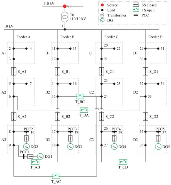
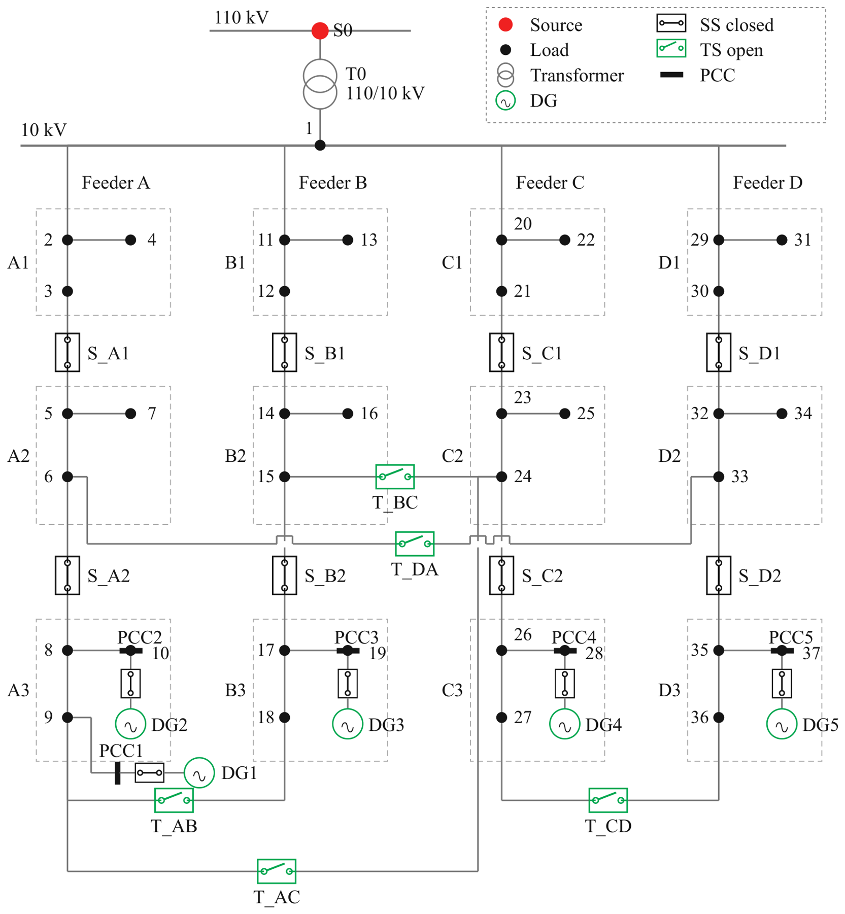
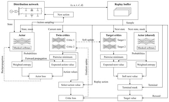
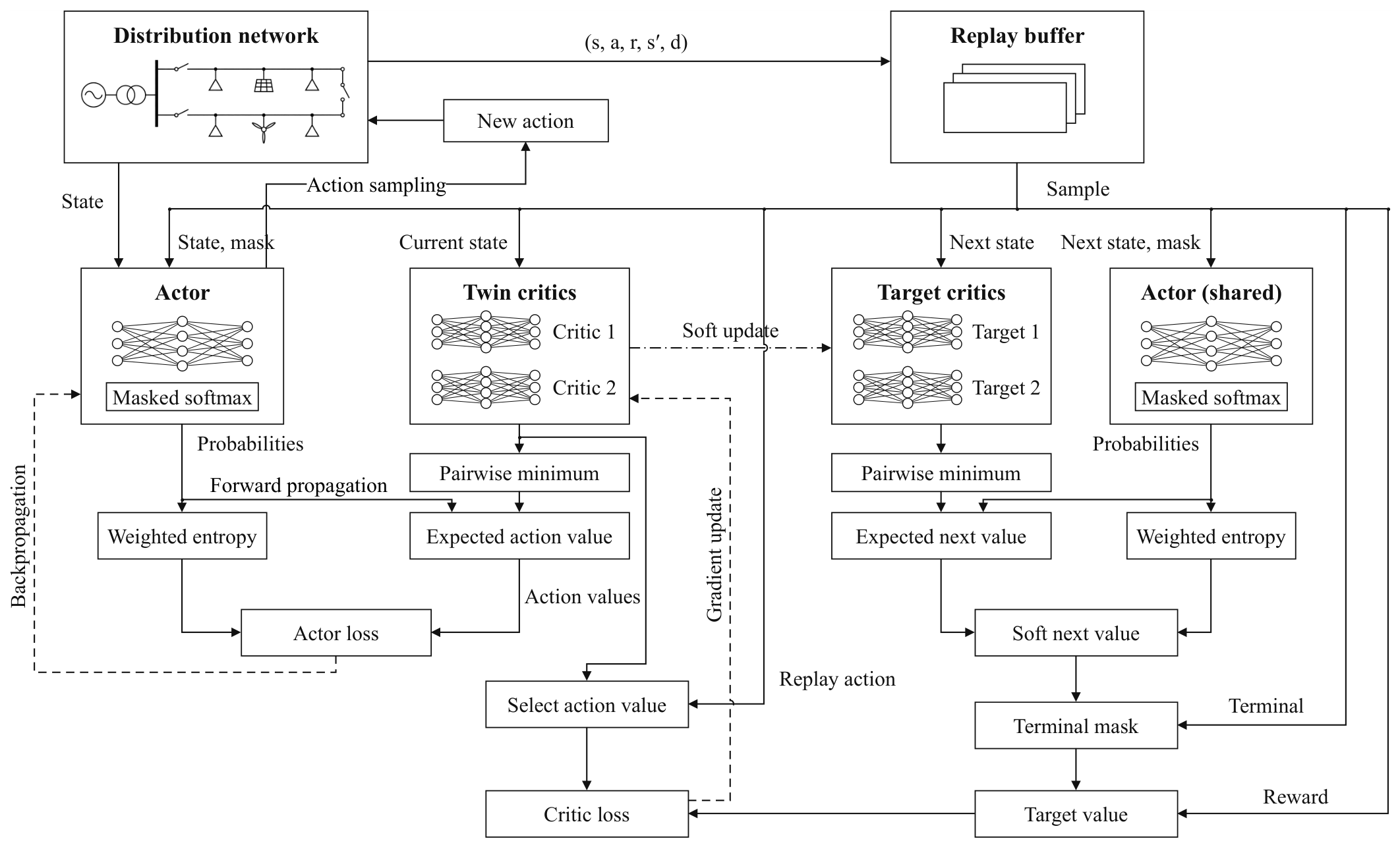
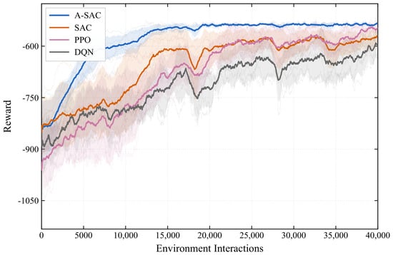
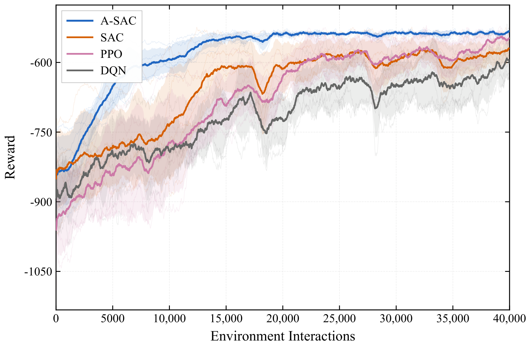
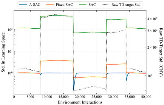
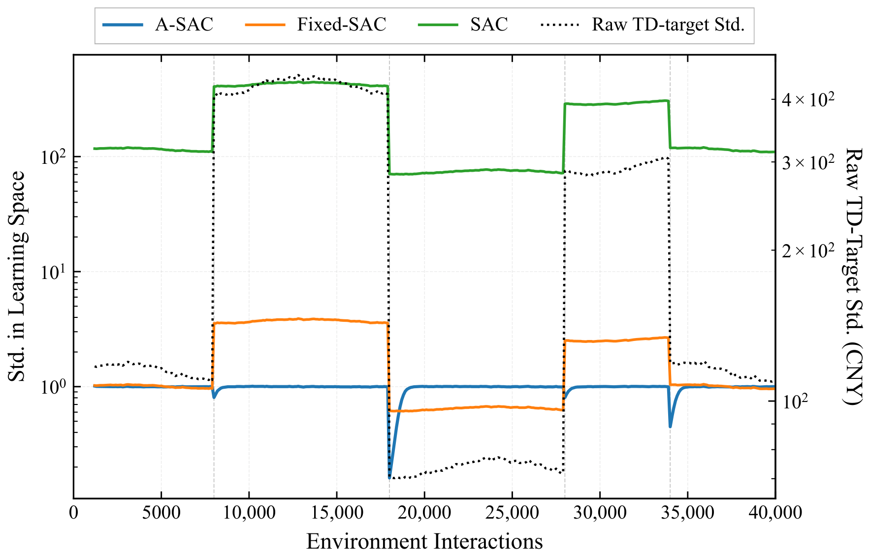
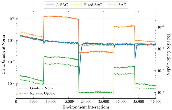
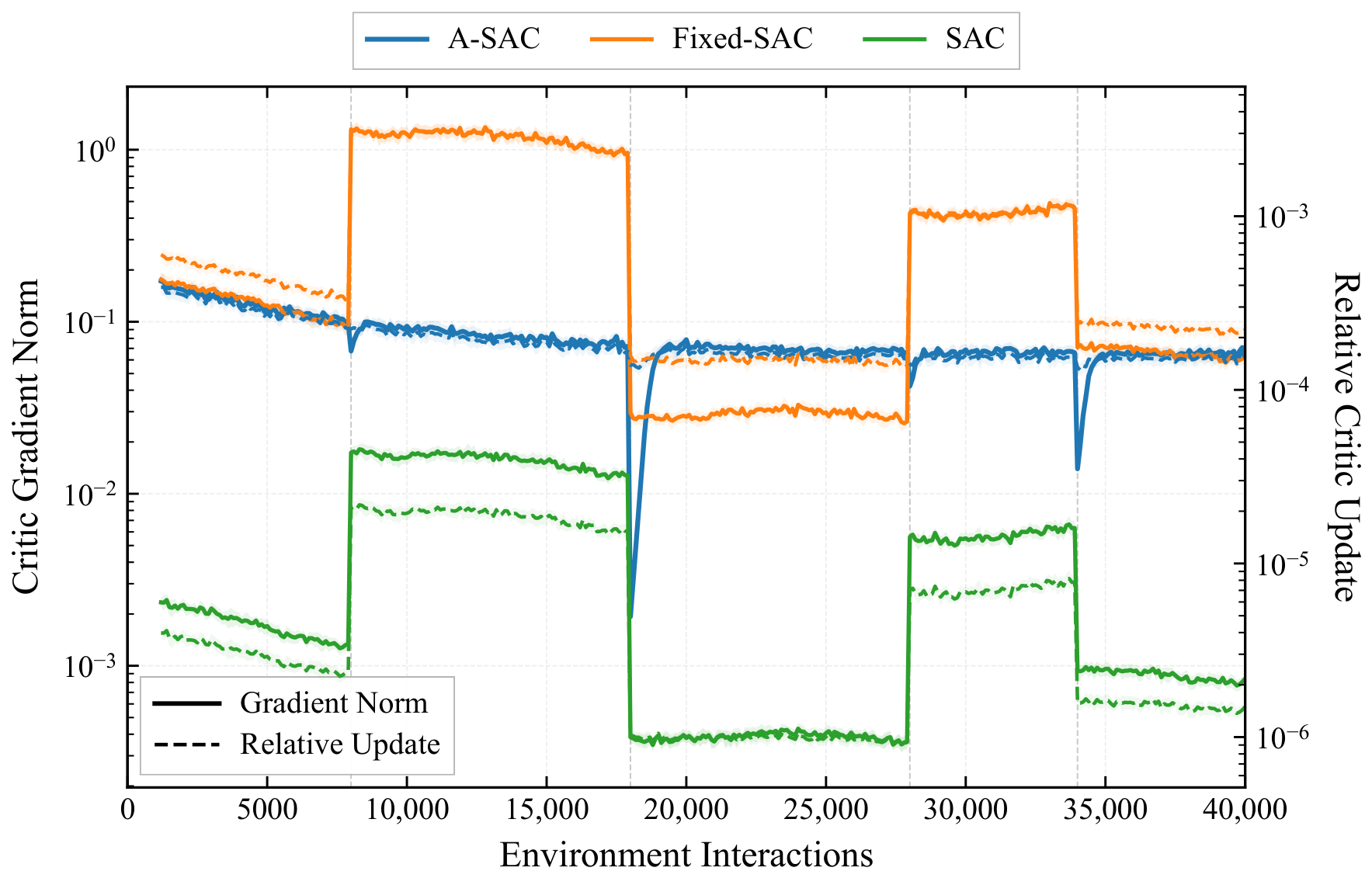
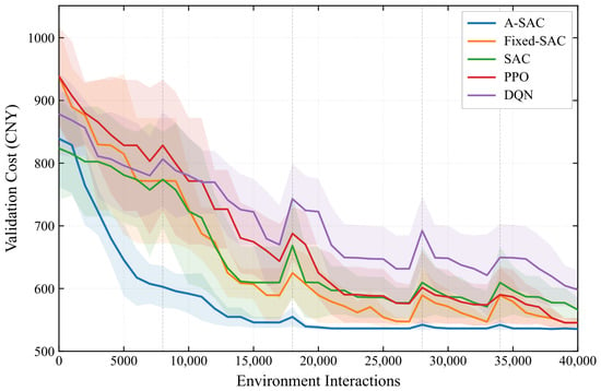
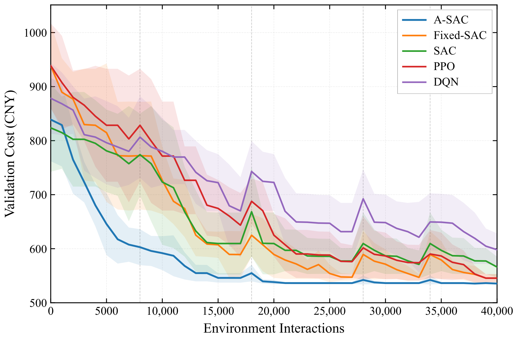
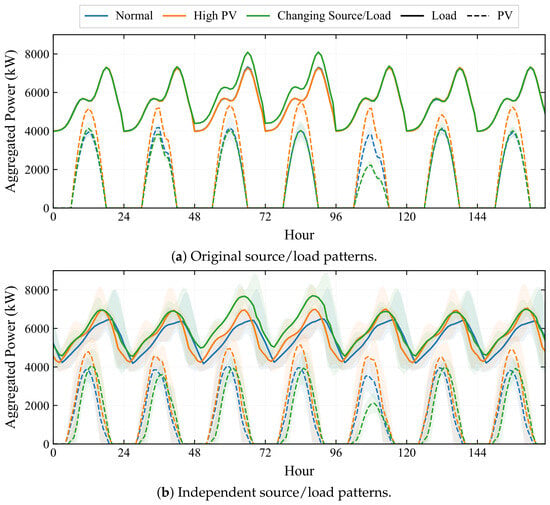
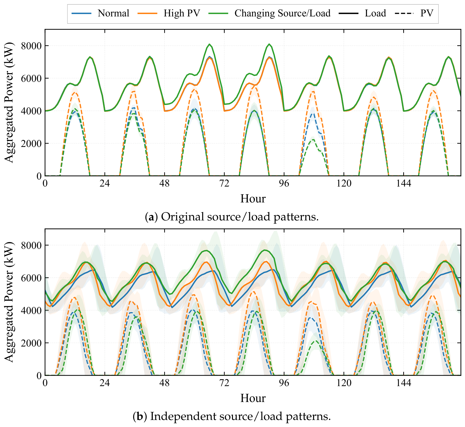
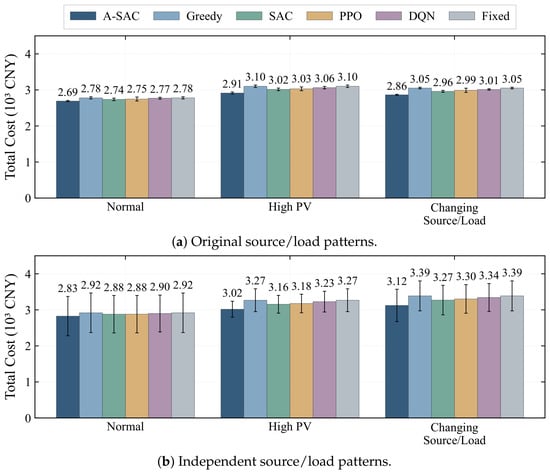
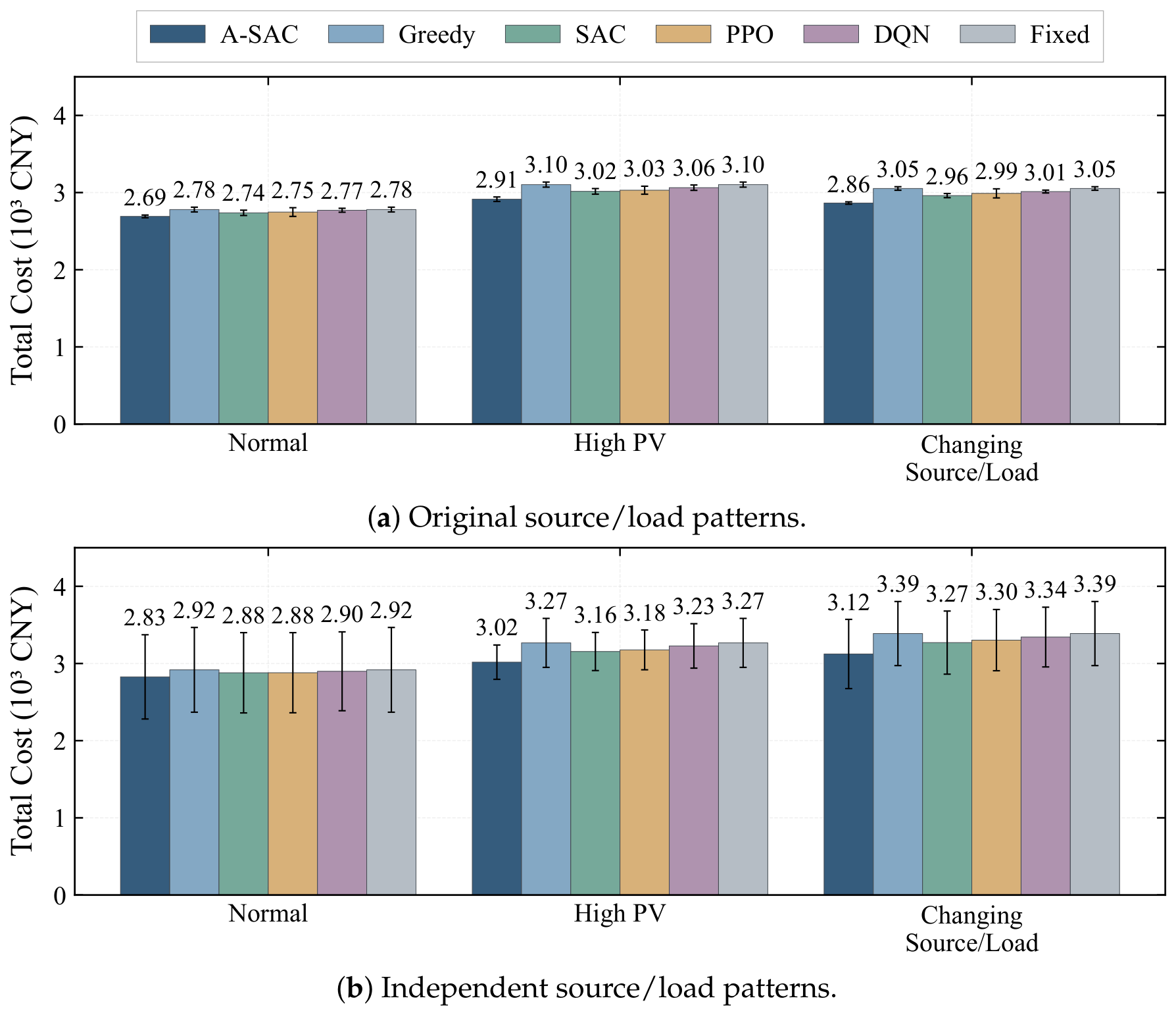
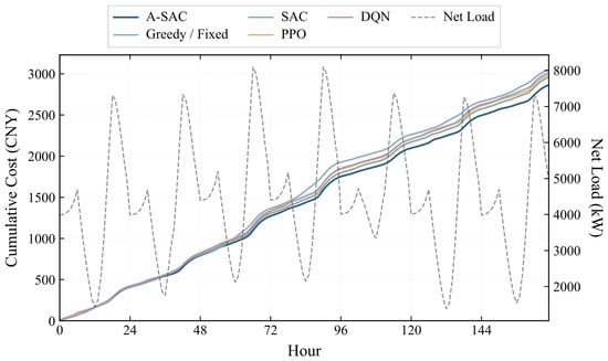
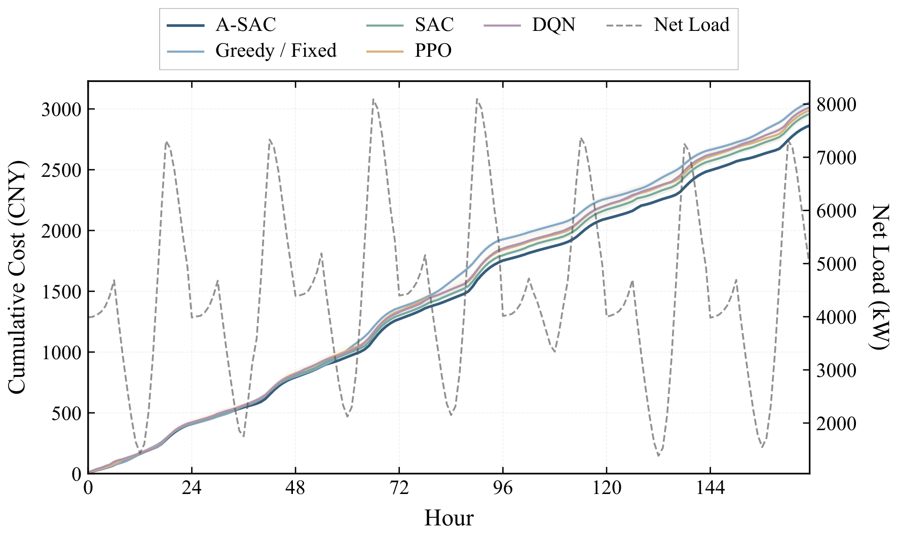
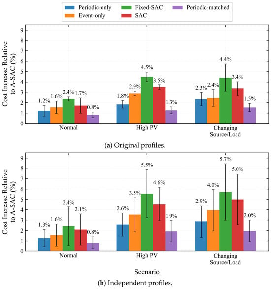
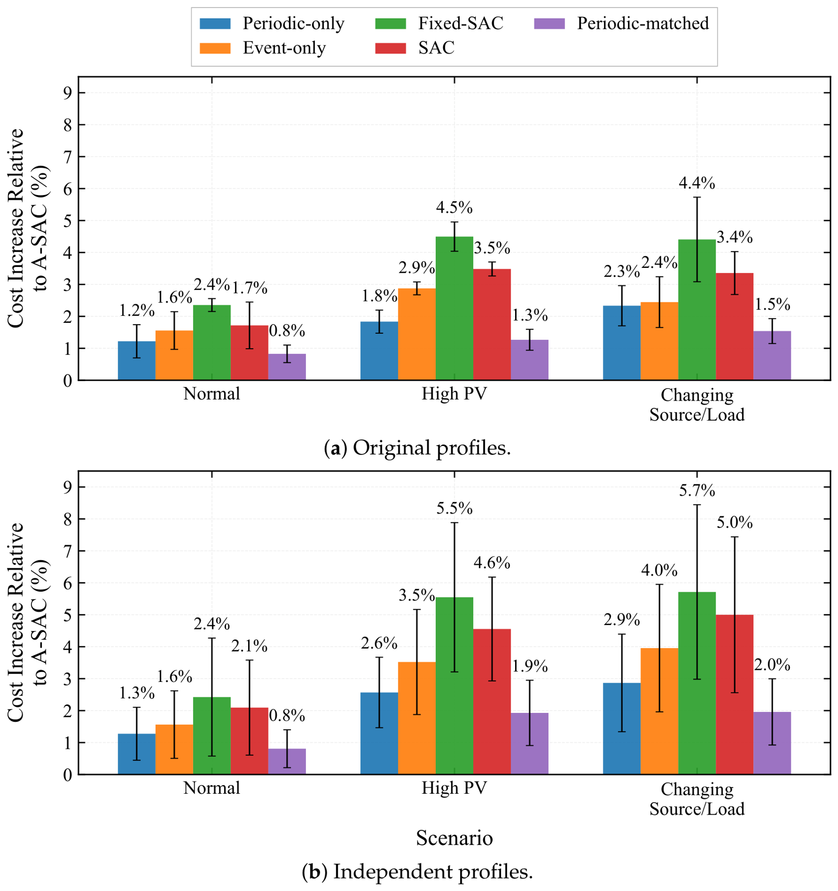
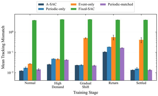
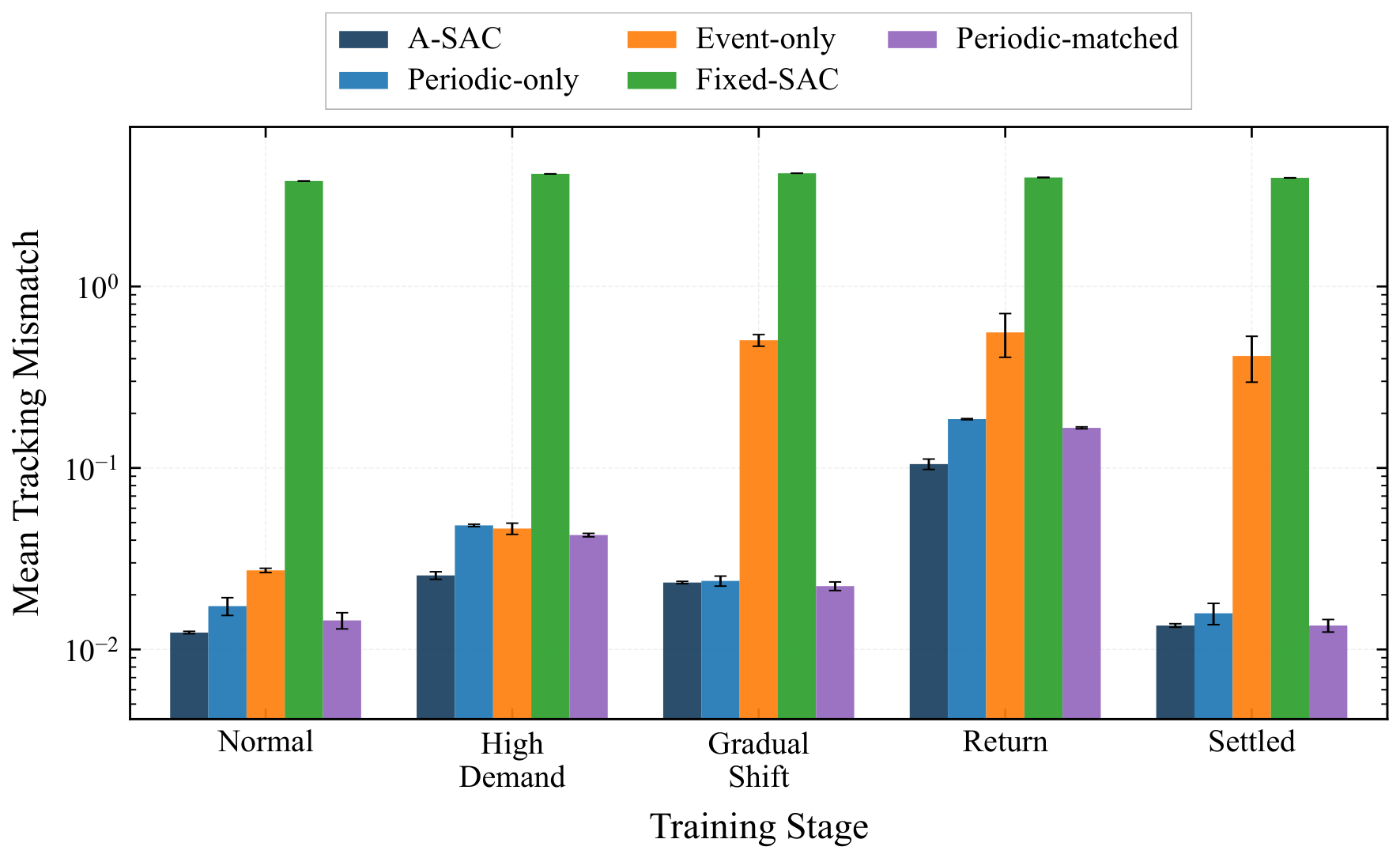
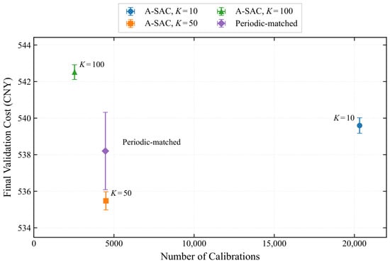
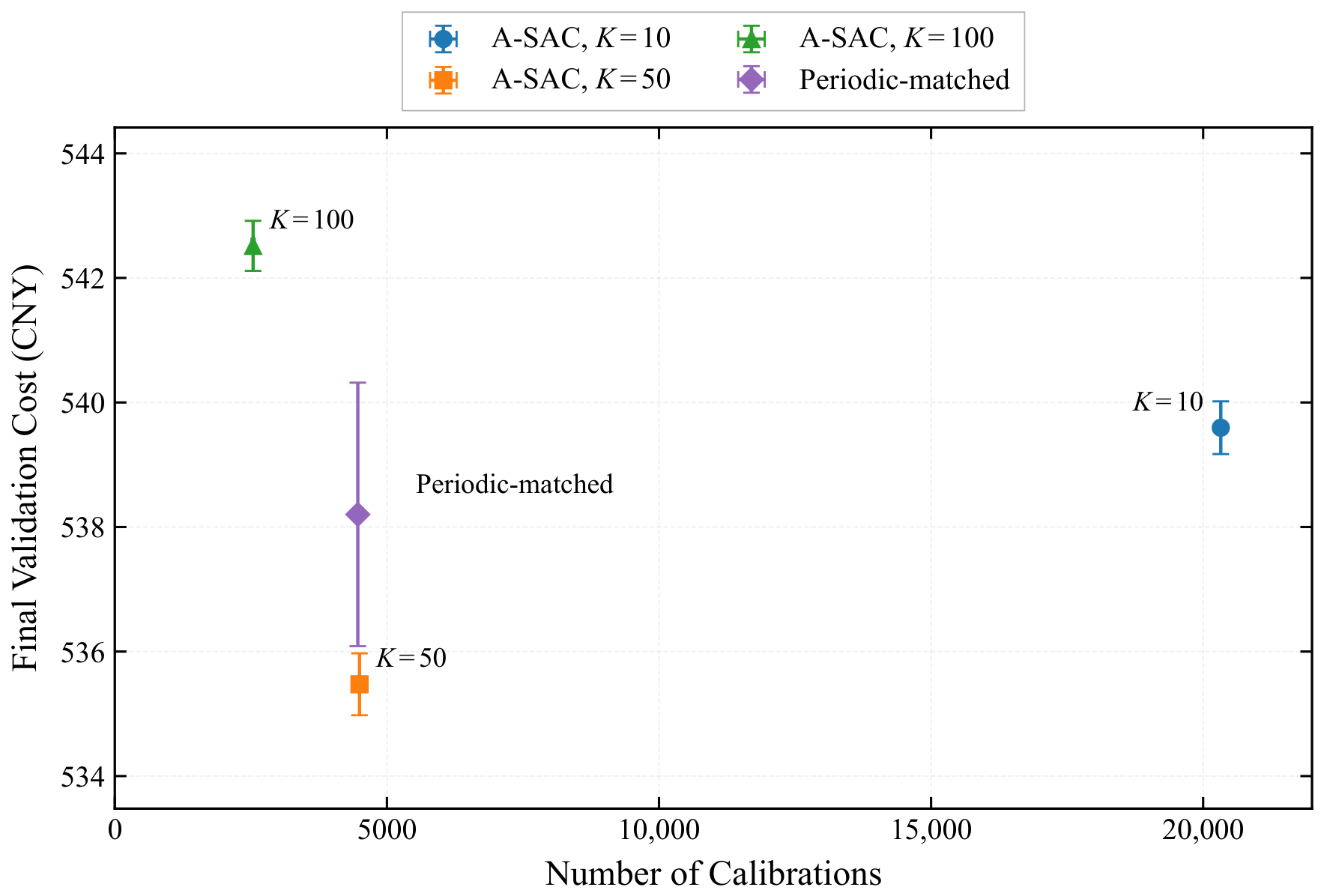

Disclaimer/Publisher’s Note: The statements, opinions and data contained in all publications are solely those of the individual author(s) and contributor(s) and not of MDPI and/or the editor(s). MDPI and/or the editor(s) disclaim responsibility for any injury to people or property resulting from any ideas, methods, instructions or products referred to in the content. |
© 2026 by the authors. Licensee MDPI, Basel, Switzerland. This article is an open access article distributed under the terms and conditions of the Creative Commons Attribution (CC BY) license.