Optimal Selection Method for Terminal-Guidance Parameters with Complex Constraints Based on the TLBO Algorithm

Abstract

Simultaneously satisfying multiple constraints while maintaining a relatively simple guidance law remains challenging in terminal guidance. This paper proposes a parameter optimization method based on teaching–learning-based optimization (TLBO). Taking proportional navigation as an example, a bias term is designed to achieve a desired impact angle and two bias term adjustment coefficients are introduced as additional optimization variables to satisfy the seeker blind-zone constraint. The lead-angle and normal acceleration rate constraints are converted into normal acceleration magnitude constraints. With impact time and impact speed as optimization objectives, TLBO is employed to optimize the initial conditions and guidance parameters. Numerical simulations demonstrate the feasibility of the proposed method, and the Monte Carlo results show that satisfactory terminal guidance performance is maintained under the specified normal-acceleration perturbations.

1. Introduction

Terminal guidance is the final phase of a missile’s attack mission and is crucial for precise target striking [1]. The key to terminal guidance control lies in designing an appropriate guidance law based on the missile-target relative kinematics equations [2]. For practical applications, the terminal guidance process must satisfy various constraint requirements [3]. Currently, common constraints include acceleration magnitude constraints, acceleration rate constraints, lead angle constraints, seeker blind zone constraints, impact speed constraints, impact angle constraints, and impact time constraints. Furthermore, compared with missiles equipped with active thrust along the velocity direction, for aerodynamic-only maneuvering missiles, only the normal acceleration is controllable, which makes the terminal guidance problem under the aforementioned complex constraints even more challenging to solve. It should be further clarified that the acceleration magnitude and acceleration rate constraints mainly consider the limits on the magnitude and rate of change of the missile’s angle of attack and sideslip angle [4]; the lead angle and seeker blind zone constraints primarily address the limitations of the missile seeker’s detection capabilities [5]; the impact speed constraint primarily considers the striking effectiveness of the missile [6]; and the impact time and impact angle constraints mainly account for multi-missile cooperative engagement scenarios [7].

To simultaneously satisfy these multiple constraints, guidance laws typically become increasingly complex, which is detrimental to their practical application. Therefore, without significantly increasing the complexity of the guidance law, optimizing the terminal guidance parameters has become a practical and feasible method to satisfy multiple constraints while ensuring the target is struck [8]. During the terminal guidance process, the initial conditions of the terminal guidance and the key parameters of the guidance law play a decisive role [9]. Under multiple constraint conditions, intelligent optimization algorithms can be used to find parameter values that optimize the objective function [10,11,12]. Common intelligent optimization algorithms include the teaching-learning-based optimization (TLBO) algorithm [10], genetic algorithm (GA) [11] and particle swarm optimization (PSO) [12]. In this study, TLBO is employed to solve the formulated parameter-selection problem.

Previous studies have addressed different subsets of terminal guidance constraints, including impact-time and impact-angle constraints [2,7,13,14], field-of-view constraints [3,5,13,14,15,16,17,18], terminal-speed requirements [6,16], and acceleration constraints [4,16]. Optimization-based guidance and parameter-selection approaches have also been investigated [8,11,12,16,19]. In particular, ref. [16] developed a three-dimensional guidance method that incorporates terminal impact-angle requirements, field-of-view and lateral-acceleration constraints, while maximizing terminal speed and minimizing flight time. However, the simultaneous treatment of prescribed impact time, prescribed impact speed, normal-acceleration magnitude and rate, lead angle, and seeker-blind-zone constraints within a proportional navigation (PN)-based parameter-optimization framework remains insufficiently investigated.

To address these issues, this paper develops a multi-constraint terminal guidance parameter-optimization framework without fundamentally altering the structure of the PN guidance law. The contributions lie in the modification of the biased PN law and the formulation of the constrained parameter-selection problem, while the standard TLBO algorithm is used only as the numerical solver. The specific contributions are as follows:

(1) From the guidance-law perspective, the biased PN guidance law is improved by introducing adjustable bias-term coefficients. By optimizing these coefficients, the prescribed impact angles can be achieved while satisfying the seeker blind-zone constraint.

(2) From the optimization-formulation perspective, the normal-acceleration-rate and lead-angle constraints are converted into implementable normal-acceleration constraints, and the terminal guidance initial conditions and guidance-law parameters are jointly selected. A normalized performance index associated with impact time and impact speed is defined, and the resulting multi-constraint parameter-selection problem is solved using TLBO.

(3) Monte Carlo simulations with normal-acceleration perturbations are conducted to evaluate the performance of the optimized parameters under the uncertainty conditions considered in this study.

2. Problem Description

This section first presents the three-dimensional relative motion equations between the missile and the target and the missile motion equations. It then describes various motion constraints that need to be considered during the terminal guidance phase, and finally provides the design objectives of this paper.

2.1. Equations of Motion

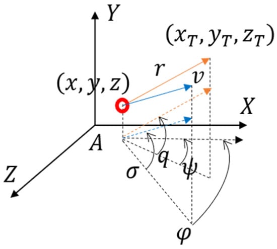
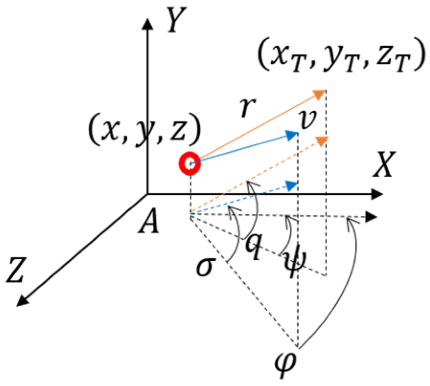
Figure 1 illustrates the three-dimensional relative motion between the missile and the target. Let $AXYZ$ denote the inertial coordinate system. $\left(x_T,y_T,z_T\right)$ and $\left(x,y,z\right)$ represent the positions of the target and the missile, respectively.

Figure 1. Schematic diagram of the three-dimensional relative kinematic relationship between missile and target.

Let $r$ denote the relative distance between the missile and the target, and $v$ denote the missile velocity. $\sigma$ is the flight-path elevation angle, and $\phi$ is the flight-path azimuth angle. $a^{\sigma }$ denotes the normal acceleration generated by aerodynamic forces to change $\sigma$, and $a^{\phi }$ denotes the normal acceleration used to change $\phi$. $a^v$ represents the acceleration along the velocity direction caused by aerodynamic drag, and $g$ is gravitational acceleration. Define $\sigma$ as positive when the velocity points above the $AXZ$ plane, and negative otherwise; $q$ is the line-of-sight (LOS) elevation angle, defined as positive when the vector from the missile position to the target position points above the $AXZ$ plane, and negative otherwise. Define $\phi$ as positive when the velocity points to the left side of the $AXY$ plane, and negative otherwise; $\psi$ is the LOS azimuth angle, defined as positive when the vector from the missile to the target points to the left side of the $AXY$ plane, and negative otherwise.

The missile-target relative kinematics equations are:

$$\left\{\begin{array}{c}\dot{r}=-v\cos \sigma \cos q\cos \left(\psi -\phi \right)-v\sin \sigma \sin q\\ r\dot{q}=-v\sin \sigma \cos q+v\cos \sigma \sin q\cos \left(\psi -\phi \right)\\ r\dot{\psi }\cos q=v\cos \sigma \sin \left(\psi -\phi \right)\end{array}\right.$$

(1)

The missile kinematics equations are:

$$\left\{\begin{array}{c}\dot{x}=v\mathit{cos}\sigma cos\phi \\ \dot{y}=v\sin \sigma \\ \dot{z}=-v\mathit{cos}\sigma sin\phi \\ \dot{v}=-a^v-g\sin \sigma \\ v\dot{\sigma }=a^{\sigma }-g\cos \sigma \\ -v\mathit{cos}\sigma \dot{\phi }=a^{\phi }\end{array}\right.$$

(2)

Remark 1.

It should be pointed out here that the missile considered in this study has no active thrust acting along the velocity direction. The complex-constrained terminal guidance process is realized entirely by designing the guidance law and optimizing the terminal guidance parameters to generate appropriate normal accelerations $a^{\sigma }$and $a^{\phi }$. Compared with the case where the missile has active thrust along the velocity direction, this paper reduces an additional design degree of freedom, undoubtedly further increasing the difficulty of target striking under complex constraints. According to aerodynamics, the changes in $a^{\sigma }$and $a^{\phi }$can be realized by changing the angle of attack $\mathsf{\alpha }$ and sideslip angle $\mathsf{\beta }$, and the aerodynamic drag $a^v$  is also related to $\mathsf{\alpha }$ and $\mathsf{\beta }$. In the simulation analysis of this paper, to account for the correlation between aerodynamic drag and aerodynamic force, without loss of generality, the following is selected:

$$a^v=\delta \left|a^{\sigma }\right|+\epsilon \left|a^{\phi }\right|$$

(3)

where $\delta$ and $\epsilon$ are positive values related to the lift coefficient, side-force coefficient and drag coefficient.

2.2. Kinematic Constraints

The entire terminal guidance process needs to satisfy multiple constraints, including the impact time constraint and impact angle constraint considering multi-missile cooperation, the impact speed constraint considering striking effect, the lead angle constraint and seeker blind zone constraint considering seeker detection capabilities, and the acceleration magnitude constraint and acceleration rate constraint considering missile maneuverability. These constraints are described below:

(1) Impact time constraint: Let the time required for the missile to hit the target be $t_f$ and $t_f^{\ast }$ be the given impact time. The impact time constraint requires:

$$t_f=t_f^{\mathrm{*}}$$

(4)

(2) Impact speed constraint: Let the velocity of the missile when it hits the target be $v_f$ and $v_f^{\ast }$ be the given impact speed. The impact speed constraint is:

$$v_f=v_f^{\mathrm{*}}$$

(5)

(3) Impact angle constraint: Let the flight path elevation angle and azimuth angle of the missile when it hits the target be ${\sigma }_f$ and ${\phi }_f$ respectively, and ${\sigma }_f^{\ast }$ and ${\phi }_f^{\ast }$ be the given impact flight path elevation angle and azimuth angle. The impact angle constraint is:

$$\left\{\begin{array}{c}{\sigma }_f={\sigma }_f^{\mathrm{*}}\\ {\phi }_f={\phi }_f^{\mathrm{*}}\end{array}\right.$$

(6)

(4) Acceleration magnitude constraint: During the terminal guidance process, the normal accelerations $a^{\sigma }$ and $a^{\phi }$ satisfy the following constraints:

$$\left\{\begin{array}{c}\left|a^{\sigma }\right|\le a_{max}^{\sigma }\\ \left|a^{\phi }\right|\le a_{max}^{\phi }\end{array}\right.$$

(7)

(5) Acceleration rate constraint: During the terminal guidance process, the normal acceleration rates ${\dot{a}}^{\sigma }$ and ${\dot{a}}^{\phi }$ satisfy the following constraints:

$$\left\{\begin{array}{c}\left|{\dot{a}}^{\sigma }\right|\le {\dot{a}}_{max}^{\sigma }\\ \left|{\dot{a}}^{\phi }\right|\le {\dot{a}}_{max}^{\phi }\end{array}\right.$$

(8)

where ${\dot{a}}_{max}^{\sigma }$ and ${\dot{a}}_{max}^{\phi }$ are the allowable maximum acceleration rates.

(6) Seeker blind zone constraint: When the missile-target distance is less than a certain value, the missile enters the seeker’s blind zone. At this time, the missile cannot obtain the relative kinematic state of the missile and target to calculate $a^{\sigma }$ and $a^{\phi }$. In this paper, when the missile is in the blind zone, $a^{\sigma }$ and $a^{\phi }$ are calculated as follows:

$$\left\{\begin{array}{c}{a}^{\sigma }=g\cos \sigma , \forall r<d\\ a^{\phi }=0, \forall r<d\end{array}\right.$$

(9)

where $d$ is the missile-target distance at which the missile enters the blind zone before hitting the target. $a^{\sigma }$ and $a^{\phi }$ do not require the missile-target relative kinematic state, and simultaneously ensure $v\dot{\sigma }=0$ and $v\mathit{cos}\sigma \dot{\phi }=0$.

(7) Lead angle constraint: Define the lead angles as $\eta =q-\sigma$ and $\mu =\psi -\phi$. The lead angle constraint is:

$$\left\{\begin{array}{c}\left|\eta \right|\le {\eta }_{max}, \forall r\ge d\\ \left|\mu \right|\le {\mu }_{max}, \forall r\ge d\end{array}\right.$$

(10)

where ${ \eta }_{max}>0$ and ${\mu }_{max}>0$ are the allowable maximum lead angles. The equalities $\left|\eta \right|={\eta }_{max}$ and $\left|\mu \right|={\mu }_{max}$ represent only the boundaries of the admissible region and hold when the corresponding constraint is active.

Remark 2.

It should be noted here that the seeker blind zone constraint mainly considers that the seeker is in a blind zone when the missile is about to hit the target, at which point the missile cannot obtain the relative kinematic state, while the lead angle constraint mainly considers the limited field of view of the seeker. Therefore, when the missile is far from the target, the missile is outside the seeker’s blind zone, and it only needs to satisfy the lead angle constraint to ensure the seeker operates normally. Similarly, when the missile is close to the target, if the seeker has entered the blind zone and cannot operate normally, the lead angle constraint does not need to be satisfied.

2.3. Design Objectives

Based on the kinematics in Equations (1) and (2) and considering the kinematic constraints (4)–(10), the design objectives are as follows:

(1) Design a PN guidance law and optimize the initial conditions of terminal guidance and guidance law parameters to satisfy the above constraint conditions while hitting the target;

(2) Further consider the inaccuracy of the nominal values of the lift coefficient, side-force coefficient, and mass parameters causing the actual normal accelerations $a^{\sigma }$ and $a^{\phi }$ to deviate from the optimized values, and evaluate the resulting terminal-guidance performance under the specified acceleration perturbations through Monte Carlo simulations.

3. Main Results

This section first presents a PN guidance law with bias terms to achieve a given impact angle; considering the seeker blind zone constraint, bias term adjustment coefficients are additionally added to the PN guidance law, so that through parameter optimization, the missile can reach the given impact angle state before entering the blind zone, i.e., $q=\sigma ={\sigma }_f^{\ast }$ and $\psi =\phi ={\phi }_f^{\ast }$; then, the acceleration magnitude constraint, acceleration rate constraint, and lead angle constraint are transformed into constraints on the acceleration magnitude executable by a computer system; on this basis, performance indices are defined considering the impact speed and impact time constraints, and the TLBO method is used to optimize the terminal guidance initial conditions and guidance law parameters, solving the terminal guidance parameter optimization problem under complex constraints.

3.1. Proportional Navigation Guidance Law Considering Impact Angle Constraint

The PN guidance law is widely used in practice, and its form is as follows:

$$\left\{\begin{array}{c}{a}_0^{\sigma }=b^{\sigma }v\dot{q}+g\cos \sigma \\ a_0^{\phi }=-b^{\phi }v\mathit{cos}\sigma \dot{\psi }\end{array}\right.$$

(11)

where $b^{\sigma }$ and $b^{\phi }$ are the PN coefficients.

To enable the missile to hit the target with the desired impact angle, a bias term is added to Equation (11), and its general form is as follows:

$$\left\{\begin{array}{c}{a}^{\sigma }=a_0^{\sigma }+a_B^{\sigma }\\ a^{\phi }=a_0^{\phi }+a_B^{\phi }\end{array}\right.$$

(12)

where $a_B^{\sigma }$ and $a_B^{\phi }$ are bias terms.

Substituting Equation (12) into Equation (2) yields:

$$\left\{\begin{array}{c}\dot{\sigma }=b^{\sigma }\dot{q}+{\displaystyle \frac{a_B^{\sigma }}{v}}\\ \dot{\phi }=b^{\phi }\dot{\psi }-{\displaystyle \frac{a_B^{\phi }}{v\mathit{cos}\sigma }}\end{array}\right.$$

(13)

From the above equation, in a very short time before hitting the target, the following relationship holds:

$$\left\{\begin{array}{c}{\displaystyle \frac{{\sigma }_f-\sigma }{∆t}}=b^{\sigma }{\displaystyle \frac{q_f-q}{∆t}}+{\displaystyle \frac{a_B^{\sigma }}{v}}\\ {\displaystyle \frac{{\phi }_f-\phi }{∆t}}=b^{\phi }{\displaystyle \frac{{\psi }_f-\psi }{∆t}}-{\displaystyle \frac{a_B^{\phi }}{v\mathit{cos}\sigma }}\end{array}\right.$$

(14)

where $q_f$ and ${\psi }_f$ are the LOS elevation and azimuth angles when hitting the target. Since $r=0$ at impact, according to Equation (1), $q_f={\sigma }_f$, ${\phi }_f={\psi }_f$; $∆t=t_f-t$ is the remaining time to go.

Rearranging Equation (14) yields:

$$\left\{\begin{array}{c}{a}_B^{\sigma }=-\left(\sigma -b^{\sigma }q+\left(b^{\sigma }-1\right){\sigma }_f\right)v/∆t\\ a_B^{\phi }=\left(\phi -b^{\phi }\psi +\left(b^{\phi }-1\right){\phi }_f\right)v\mathit{cos}\sigma /∆t\end{array}\right.$$

(15)

In a very short time before hitting the target, the remaining time to go satisfies:

$$∆t=r/v$$

(16)

Combining Equations (6), (15), and (16), the PN guidance law with bias terms considering the impact angle constraint is obtained as follows:

$$\left\{\begin{array}{c}{a}^{\sigma }=a_0^{\sigma }+a_B^{\sigma }=b^{\sigma }v\dot{q}+g\cos \sigma -\left(\sigma -b^{\sigma }q+\left(b^{\sigma }-1\right){\sigma }_f^{\mathrm{*}}\right)v^2/r\\ a^{\phi }=a_0^{\phi }+a_B^{\phi }=-b^{\phi }v\mathit{cos}\sigma \dot{\psi }+\left(\phi -b^{\phi }\psi +\left(b^{\phi }-1\right){\phi }_f^{\mathrm{*}}\right)v^2\mathit{cos}\sigma /r\end{array}\right.$$

(17)

3.2. Improved Guidance Law Further Considering Seeker Blind Zone Constraint

Considering the seeker blind zone constraint, after the missile enters the seeker’s blind zone, $v\dot{\sigma }=0$ and $v\mathit{cos}\sigma \dot{\phi }=0$. Therefore, the missile needs to reach the terminal impact angle state in advance, i.e., $q=\sigma ={\sigma }_f^{\ast }$ and $\psi =\phi ={\phi }_f^{\ast }$. For the biased PN guidance law, coefficients $b^{\sigma }$ and $b^{\phi }$ need to make the lead angles $\eta$ and $\mu$ approach zero. In addition, under the action of the biased PN guidance law (17), one can obtain:

$$\left\{\begin{array}{c}\dot{\sigma }=b^{\sigma }\dot{q}-\left(\sigma -b^{\sigma }q+\left(b^{\sigma }-1\right){\sigma }_f^{\mathrm{*}}\right)v/r\\ \dot{\phi }=b^{\phi }\dot{\psi }-\left(\phi -b^{\phi }\psi +\left(b^{\phi }-1\right){\phi }_f^{\mathrm{*}}\right)v/r\end{array}\right.$$

Therefore, $\sigma -b^{\sigma }q$ converges to $\left(1-b^{\sigma }\right){\sigma }_f^{\ast }$, and $\phi -b^{\phi }\psi$ converges to $\left(1-b^{\phi }\right){\phi }_f^{\ast }$. To make the convergence speed adjustable, bias term adjustment coefficients $l^{\sigma }$ and $l^{\phi }$ are added to the biased PN law (17) as follows:

$$\left\{\begin{array}{c}{a}^{\sigma }=b^{\sigma }v\dot{q}+g\cos \sigma -l^{\sigma }\left(\sigma -b^{\sigma }q+\left(b^{\sigma }-1\right){\sigma }_f^{\mathrm{*}}\right)v^2/r\\ a^{\phi }=-b^{\phi }v\mathit{cos}\sigma \dot{\psi }+l^{\phi }\left(\phi -b^{\phi }\psi +\left(b^{\phi }-1\right){\phi }_f^{\mathrm{*}}\right)v^2\mathit{cos}\sigma /r\end{array}\right.$$

(18)

At this time:

$$\left\{\begin{array}{c}\dot{\sigma }=b^{\sigma }\dot{q}-l^{\sigma }\left(\sigma -b^{\sigma }q+\left(b^{\sigma }-1\right){\sigma }_f^{\mathrm{*}}\right)v/r\\ \dot{\phi }=b^{\phi }\dot{\psi }-l^{\phi }\left(\phi -b^{\phi }\psi +\left(b^{\phi }-1\right){\phi }_f^{\mathrm{*}}\right)v/r\end{array}\right.$$

Therefore, the convergence speed of $\sigma -b^{\sigma }q$ to $\left(1-b^{\sigma }\right){\sigma }_f^{\ast }$ and $\phi -b^{\phi }\psi$ to $\left(1-b^{\phi }\right){\phi }_f^{\ast }$ can be adjusted by adjusting the values of $l^{\sigma }$ and $l^{\phi }$.

Thus, for the PN guidance law (18), coefficients $b^{\sigma }$, $b^{\phi }$, $l^{\sigma }$ and $l^{\phi }$ can be adjusted so that the missile realizes $q=\sigma ={\sigma }_f^{\ast }$ and $\psi =\phi ={\phi }_f^{\ast }$ before entering the seeker’s blind zone.

3.3. Normal Acceleration Magnitude Constraint

The normal acceleration magnitude constraint is implemented in the computer system as follows:

If $a^{\sigma }\left[k\right]>a_{max}^{\sigma }$,

$$a^{\sigma }\left[k\right]=a_{max}^{\sigma };$$

If $a^{\sigma }\left[k\right]<-a_{max}^{\sigma }$,

$$a^{\sigma }\left[k\right]=-a_{max}^{\sigma };$$

Otherwise, $a^{\sigma }\left[k\right]$ remains unchanged.

If $a^{\phi }\left[k\right]>a_{max}^{\phi }$,

$$a^{\phi }\left[k\right]=a_{max}^{\phi };$$

If $a^{\phi }\left[k\right]<-a_{max}^{\phi }$,

$$a^{\phi }\left[k\right]=-a_{max}^{\phi };$$

Otherwise, $a^{\phi }\left[k\right]$ remains unchanged.

Here, $a^{\sigma }\left[k\right]$ is the discrete-time variable for $a^{\sigma }$. Defining $a^{\sigma }\left(t\right)$ as the continuous-time variable for $a^{\sigma }$, $a^{\sigma }\left[k\right]=a^{\sigma }\left(k{T}_s\right)$, $k=\mathrm{1,2},\dots$; $T_s$ is the control period of the digital control system. $a^{\phi }\left[k\right]$ is the discrete-time variable for $a^{\phi }$.

3.4. Normal Acceleration Rate Constraint

The normal acceleration rate constraint is implemented in the computer system as follows:

If ${\displaystyle \frac{a^{\sigma }\left[k\right]-a^{\sigma }\left[k-1\right]}{T_s}}>{\dot{a}}_{max}^{\sigma }$,

$$a^{\sigma }\left[k\right]=a^{\sigma }\left[k-1\right]+{\dot{a}}_{max}^{\sigma }{T}_s;$$

If ${\displaystyle \frac{a^{\sigma }\left[k\right]-a^{\sigma }\left[k-1\right]}{T_s}}<-{\dot{a}}_{max}^{\sigma }$,

$$a^{\sigma }\left[k\right]=a^{\sigma }\left[k-1\right]-{\dot{a}}_{max}^{\sigma }{T}_s;$$

Otherwise, $a^{\sigma }\left[k\right]$ remains unchanged.

If ${\displaystyle \frac{a^{\phi }\left[k\right]-a^{\phi }\left[k-1\right]}{T_s}}>{\dot{a}}_{max}^{\phi }$,

$$a^{\phi }\left[k\right]=a^{\phi }\left[k-1\right]+{\dot{a}}_{max}^{\phi }{T}_s;$$

If ${\displaystyle \frac{a^{\phi }\left[k\right]-a^{\phi }\left[k-1\right]}{T_s}}<-{\dot{a}}_{max}^{\phi }$,

$$a^{\phi }\left[k\right]=a^{\phi }\left[k-1\right]-{\dot{a}}_{max}^{\phi }{T}_s;$$

Otherwise, $a^{\phi }\left[k\right]$ remains unchanged.

3.5. Lead Angle Constraint

The lead angle constraint is implemented in the computer system as follows:

If $\widehat{q}\left[k+1\right]-\widehat{\sigma }\left[k+1\right]>{\eta }_{max}$,

$$a^{\sigma }\left[k\right]={\displaystyle \frac{\widehat{q}\left[k+1\right]-{\eta }_{max}-\sigma \left[k\right]}{T_s}}v\left[k\right]+g\cos \sigma \left[k\right];$$

If $\widehat{q}\left[k+1\right]-\widehat{\sigma }\left[k+1\right]<-{\eta }_{max}$,

$$a^{\sigma }\left[k\right]={\displaystyle \frac{\widehat{q}\left[k+1\right]+{\eta }_{max}-\sigma \left[k\right]}{T_s}}v\left[k\right];$$

Otherwise, $a^{\sigma }\left[k\right]$ remains unchanged.

If $\widehat{\psi }\left[k+1\right]-\widehat{\phi }\left[k+1\right]>{\mu }_{max}$,

$$a^{\phi }\left[k\right]=-{\displaystyle \frac{\widehat{\psi }\left[k+1\right]-{\mu }_{max}-\phi \left[k\right]}{T_s}}v\left[k\right]\mathit{cos}\sigma \left[k\right];$$

If $\widehat{\psi }\left[k+1\right]-\widehat{\phi }\left[k+1\right]<-{\mu }_{max}$,

$$a^{\phi }\left[k\right]=-{\displaystyle \frac{\widehat{\psi }\left[k+1\right]+{\mu }_{max}-\phi \left[k\right]}{T_s}}v\left[k\right]\mathit{cos}\sigma \left[k\right];$$

Otherwise, $a^{\phi }\left[k\right]$ remains unchanged.

Here,

$$\widehat{\sigma }\left[k+1\right]=\sigma \left[k\right]+T_s{\displaystyle \frac{a^{\sigma }\left[k\right]-g\cos \sigma \left[k\right]}{v\left[k\right]}}$$

$$\begin{array}{cc}\hfill \widehat{q}\left[k+1\right]=q\left[k\right]-& T_s{\displaystyle \frac{v\left[k\right]}{r\left[k\right]}}\mathit{sin}\sigma \left[k\right]\mathit{cos}q\left[k\right]\hfill \\ & +T_s{\displaystyle \frac{v\left[k\right]}{r\left[k\right]}}\mathit{cos}\sigma \left[k\right]\mathit{sin}q\left[k\right]cos\left(\psi \left[k\right]-\phi \left[k\right]\right)\hfill \end{array}$$

$$\widehat{\phi }\left[k+1\right]=\phi \left[k\right]-T_s{\displaystyle \frac{a^{\phi }\left[k\right]}{v\left[k\right]\mathit{cos}\sigma \left[k\right]}}$$

$$\widehat{\psi }\left[k+1\right]=\psi \left[k\right]+T_s{\displaystyle \frac{v\left[k\right]}{r\left[k\right]}}{\displaystyle \frac{\cos \sigma \left[k\right]}{\cos q\left[k\right]}}\mathrm{s}\mathrm{i}\mathrm{n}\left(\psi \left[k\right]-\phi \left[k\right]\right)$$

$$\sigma \left[k\right],q\left[k\right],v\left[k\right],r\left[k\right],\phi \left[k\right],\psi \left[k\right]\mathrm{are} \mathrm{the} \mathrm{discrete}‐\mathrm{time} \mathrm{variables} \mathrm{for} \sigma ,q,v,r,\phi ,\psi .$$

3.6. Performance Index Design Considering Impact Speed and Time Constraints

The constraints considered in this study are handled in different ways. The impact-angle requirement is incorporated into the biased PN guidance law in Equation (18). The normal-acceleration magnitude, normal-acceleration rate, and lead-angle constraints are enforced through the constraint-handling procedures described in Section 3.3, Section 3.4 and Section 3.5, while the seeker blind-zone condition is handled according to Equation (9). Therefore, impact time and impact speed are the remaining terminal quantities included in the optimization objective.

To realize the impact time constraint, the following performance index can be defined:

$$Q_t=\left|t_f/T_s-t_f^{\mathrm{*}}/T_s\right|$$

To realize the impact speed constraint, the following performance index can be defined:

$$Q_v=\left|v_f-v_f^{\mathrm{*}}\right|$$

To satisfy both the impact time constraint and the impact speed constraint, the above two performance indices are normalized and summed to obtain the new performance index as follows:

$$Q=\left|t_f-t_f^{\mathrm{*}}\right|/t_f^{\mathrm{*}}+\left|v_f-v_f^{\mathrm{*}}\right|/v_f^{\mathrm{*}}$$

(19)

Remark 3.

The two terms in Equation (19) are normalized by their prescribed values, making them dimensionless and placing them on a common scale. Equal weights are assigned because impact time and impact speed are treated with equal importance in this study. Equation (19) ranks candidate solutions by their impact-time and impact-speed errors and is not a complete measure of constraint satisfaction. The acceptability of a candidate solution therefore requires separate verification of the target-hitting condition and the terminal and path constraints in Equations (4)–(10).

3.7. Teaching-Learning-Based Optimization Algorithm

The present problem involves the simultaneous optimization of ten initial-condition and guidance-law parameters under multiple terminal and path constraints. The standard TLBO algorithm is adopted because it requires relatively few algorithm-specific control parameters, thereby reducing the additional parameter-tuning effort. Its implementation consists of initialization, the teacher phase, and the learner phase, as briefly described below.

(1) Initialization Part:

Define the population size $L$ and the iteration number $N$.

The number of optimized parameters is $h$, i.e., $\mathit{S}\mathit{t}=\left[{St}_1,\dots {St}_h\right]$.

The range of optimized parameters is ${St}_j\in \left[\underset{\_}{{St}_j},\overline{{St}_j}\right],j=1,\dots ,h$.

The $i$-th student ${\mathit{S}\mathit{t}}_i=\left[{St}_{i1},\dots {St}_h\right],i=1,\dots ,L$ can be initialized as:

$${St}_{ij}=rand·\left(\overline{{St}_j}-\underset{\_}{{St}_j}\right)+\underset{\_}{{St}_j}$$

(20)

where $rand$ represents a uniformly distributed random number in the range $\left[0, 1\right]$.

(2) Teacher Phase:

During the teacher phase, each individual is updated toward the current best solution according to:

$${St}_{ij}^{new}={St}_{ij}^{old}+rand·\left(T_j-T_F·{Mean}_j\right)$$

(21)

where ${St}_{ij}^{old}$ and ${St}_{ij}^{new}$ represent the status of each student before and after learning, $T_j$ is the optimal value of the entire class for the $j$-th parameter (teacher), ${Mean}_j$ is the average value of the entire class for the $j$-th parameter. $T_F$ is the teaching factor, defined as:

$$T_F=round(1+rand)$$

(22)

where $round\left(·\right)$ means rounding to the nearest integer.

If the updated individual is better than the original individual, the original individual will be replaced by the new individual, thus ensuring the population develops in a better direction.

(3) Learner Phase:

During the learner phase, each individual randomly selects another individual from the population. The update direction is determined by comparing their objective-function values, and the individual is updated according to:

$${St}_{ij}^{new}=\left\{\begin{array}{c}{St}_{ij}^{old}+rand·\left({St}_{cj}-{St}_{ij}^{old}\right) if Q\left({St}_{cj}\right)<Q\left({St}_{ij}^{old}\right)\\ {St}_{ij}^{old}+rand·\left({St}_{ij}^{old}-{St}_{cj}\right) if Q\left({St}_{ij}^{old}\right)<Q\left({St}_{cj}\right)\end{array}\right.$$

(23)

where ${St}_{cj}$ is the learning partner randomly selected by ${St}_{ij}$ from the class, with index $c$. $Q\left(·\right)$ represents the objective function. Similar to the teacher phase, if the updated individual is better than the original individual, the original individual is replaced by the new individual to ensure the population evolves in a better direction.

The pseudocode of the TLBO algorithm is shown in Algorithm 1.

Algorithm 1: Teaching-Learning-Based Optimization Algorithm

Input: Define population size L, iteration number N, optimization parameter number $h$, i.e., $\mathit{S}\mathit{t}=\left[{St}_1,\dots {St}_h\right]$, optimization parameter range ${St}_j\in \left[\underset{\_}{{St}_j},\overline{{St}_j}\right], j=1,\dots ,h$.

Output: Optimal solution ${\mathit{S}\mathit{t}}^{best}.$

Initialization Phase:

Initialize the student solutions according to formula (20);

Set o $=1$;

while $o\le N$

Teacher Phase:

Calculate the average grade of all students, find the optimal solution;

for $i=1:L$

(1) Set the optimal solution as the teacher and update the student solution according to (21);

(2) If the updated individual is better than the original one, replace the original individual with the new one;

end

Learner Phase:

for $i=1:L$

(1) Students conduct mutual learning and improvement according to formula (23);

(2) If the updated individual is better than the original one, replace the original individual with the new one;

end

If the stopping criteria are met, then stop; otherwise, $o=o+1$.

end

3.8. Solving Parameter Optimization Problem Based on TLBO Algorithm

There are two categories of terminal guidance parameters: the first category is the terminal guidance initial conditions, including $x_0$, $y_0$, $z_0$, $v_0$, ${\sigma }_0$, ${\phi }_0$, $q_0,{\psi }_0,{\eta }_0$, ${\mu }_0$, $r_0$; the second category is the PN coefficients, including $b^{\sigma }$, $b^{\phi }$, $l^{\sigma }$, $l^{\phi }$.

Given $\left(x_T,y_T,z_T\right)$ and $q_0$, ${\psi }_0$ and $r_0$, the variables $x_0$, $y_0$, $z_0$ are determined. Similarly, given ${\sigma }_0$, ${\phi }_0$, ${\eta }_0$, ${\mu }_0$, the variables $q_0$ and ${\psi }_0$ are determined. Therefore, this paper selects $v_0$, ${\sigma }_0$, ${\phi }_0$, ${\eta }_0,{\mu }_0,r_0$, $b^{\sigma }$, $b^{\phi }$, $l^{\sigma }$, $l^{\phi }$ as parameters to be optimized, i.e.,

$$\mathit{S}\mathit{t}=\left[{St}_1,\dots {St}_{10}\right]=\left[v_0,{\sigma }_0,{\phi }_0,{\eta }_0,{\mu }_0,r_0,b^{\sigma },b^{\phi },l^{\sigma },l^{\phi }\right]$$

According to the requirements of the TLBO algorithm, the parameter ranges are predefined as ${St}_j\in \left[\underset{\_}{{St}_j},\overline{{St}_j}\right], j=1,\dots ,10$. Based on all the derivations above, the optimization problem is defined as follows:

Multi-constraint terminal guidance parameter optimization problem: Given target position $\left(x_T,y_T,z_T\right)$, specify the required impact angles as ${\sigma }_f^{\ast }$ and ${\phi }_f^{\ast }$, set $a_{max}^{\sigma }$, $a_{max}^{\phi }$, ${\dot{a}}_{max}^{\sigma }$, ${\dot{a}}_{max}^{\phi }$, ${\eta }_{max}$, ${\mu }_{max}$ and $d$, optimize the PN parameters $b^{\sigma }$, $b^{\phi }$, $l^{\sigma }$, $l_{\phi }$ and initial speed $v_0$, initial flight path angles ${\sigma }_0$ and ${\phi }_0$, initial lead angles ${\eta }_0$ and ${\mu }_0,$ and initial missile-target distance $r_0$ to satisfy the impact time $t_f=t_f^{\ast }$ and impact speed $v_f=v_f^{\ast }.$ Namely:

$$\underset{{\mathit{St}}_j\in \left[\underset{\_}{{\mathit{St}}_j},\overline{{\mathit{St}}_j}\right],j=1,\dots ,10}{\min }Q$$

(24)

s.t.

Missile kinematics equations: Equation (2);

Missile-target relative kinematics equations: Equation (1);

Proportional navigation guidance law: Equation (18);

Normal acceleration magnitude constraint: Equation (7);

Normal acceleration rate constraint: Equation (8);

Seeker blind zone constraint: Equation (9);

Lead angle constraint: Equation (10).

4. Simulation Analysis

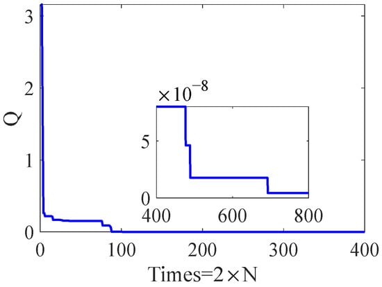
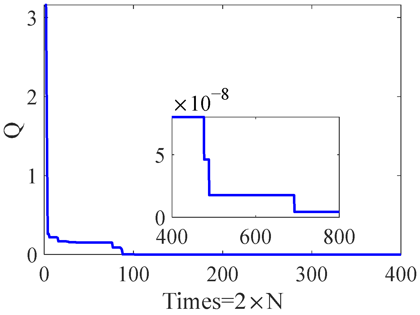
The following numerical example evaluates the proposed method under the specified initial conditions and constraint settings. In the simulation, set the target position as $\left(x_T,y_T,z_T\right)=\left(\mathrm{9000,9000},-9000\right)$ m, the given impact angles ${\sigma }_f^{\ast }=-85$ deg, ${\phi }_f^{\ast }=30$ deg, the given impact time $t_f^{\ast }=27 \mathrm{s}$, and the given impact speed $v_f^{\ast }=360 \mathrm{m}/\mathrm{s}$, $a_{max}^{\sigma }=a_{max}^{\phi }=30 \mathrm{m}$/${\mathrm{s}}^2$, ${\dot{a}}_{max}^{\sigma }={\dot{a}}_{max}^{\phi }=1000 \mathrm{m}$/${\mathrm{s}}^3$, ${\eta }_{max}={\mu }_{max}=60$ deg, $d=200 \mathrm{m}$. For the aerodynamic drag-related coefficients shown in (3), $\delta =0.2$ and $\epsilon =0.1$. The optimization ranges for each parameter are selected as follows: $v_0\in \left[100,500\right] \mathrm{m}/\mathrm{s}$, ${\sigma }_0\in \left[-30,30\right] \mathrm{d}\mathrm{e}\mathrm{g}$, ${\phi }_0\in \left[-30,30\right] \mathrm{d}\mathrm{e}\mathrm{g}$, ${\eta }_0\in \left[-60,60\right] \mathrm{d}\mathrm{e}\mathrm{g}$, ${\mu }_0\in \left[-60,60\right] \mathrm{d}\mathrm{e}\mathrm{g}$, $r_0\in \left[6000,9000\right] \mathrm{m}$, $b^{\sigma }\in \left[2,100\right]$, $b^{\phi }\in \left[2,100\right]$, $l^{\sigma }\in \left[1,3\right]$, $l^{\phi }\in \left[1,3\right]$. The TLBO algorithm population size is set to $L=5$, and the number of iterations is $N=400$. In addition to the maximum iteration count stated above, the optimization stopped early if a newly improved best objective value fell below ${10}^{-9}$ after the first iteration. If the simulation results do not satisfy the specified requirements, the parameters are adjusted and the calculation is repeated. Solving problem (24) using the TLBO algorithm, the change curve of the performance index (19) during the optimization process is shown in Figure 2, and the optimization results of the parameters are shown in Table 1. Figure 2 shows that the performance index converges to a value on the order of ${10}^{-9}$, indicating that the impact-time and impact-speed errors are small and that the corresponding requirements are satisfied. The remaining terminal and path constraints are verified separately using the resulting trajectory.

Figure 2. Evolution of the performance index during optimization.

Table 1. Parameter optimization results.

Optimized Parameter	Optimization Result	Optimized Parameter	Optimization Result
$r_0$ [m]	6.3709 $\times {10}^3$	${\sigma }_0$ [deg]	−13.8666
$v_0$ [m/s]	239.5410	${\phi }_0$ [deg]	−0.9072
${\eta }_0$ [deg]	−45.8608	${\mu }_0$ [deg]	7.0109
$b^{\sigma }$	44.8497	$l^{\sigma }$	2.2892
$b^{\phi }$	16.9663	$l^{\phi }$	2.2974

4.1. Terminal Guidance Process Analysis Under Optimized Parameters

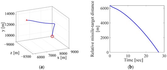
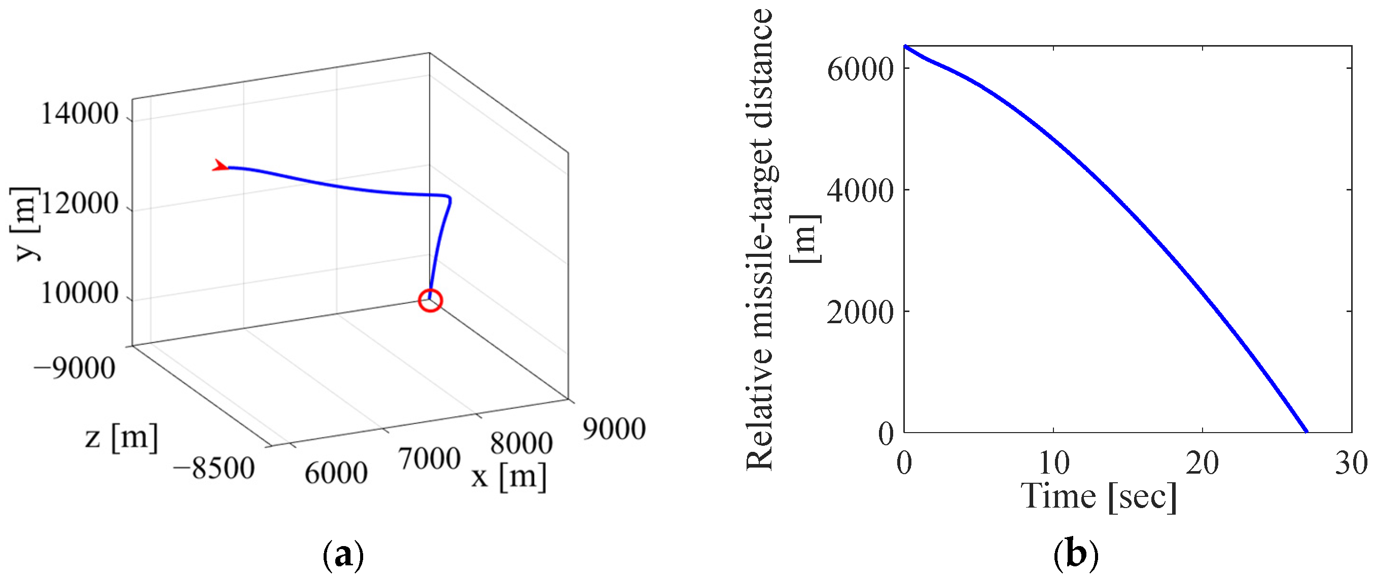
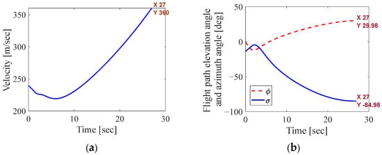
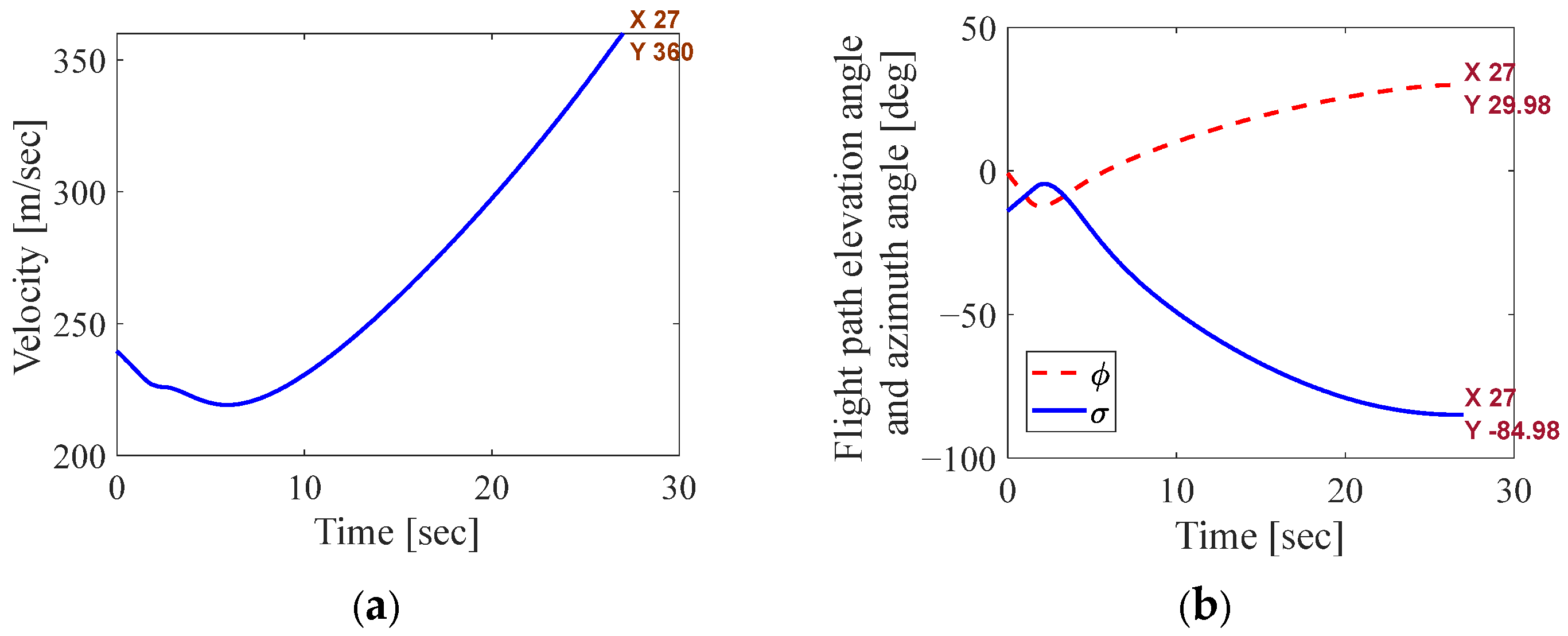
Figure 3a shows the 3D trajectory of the missile during the terminal guidance process under the optimized parameters.Figure 3b, Figure 4 and Figure 5 show the changes of various missile variables over time during the terminal guidance process under the optimized parameters.

Figure 3. (a) Three-dimensional missile trajectory and (b) change of relative missile-target distance over time during terminal guidance under optimized parameters. In (a), the red arrowhead indicates the starting point, and the red circle indicates the endpoint of the trajectory.

Figure 4. (a) Change of velocity over time and (b) changes of flight path elevation angle and azimuth angle over time during terminal guidance under optimized parameters.

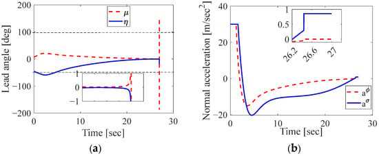
Figure 5. (a) Changes of lead angles over time and (b) changes of normal accelerations over time during terminal guidance under optimized parameters.

Figure 3b first shows that the designed biased PN guidance law under optimized parameters can hit the target subject to constraints on acceleration magnitude, acceleration rate, lead angle, and seeker blind zone. Figure 4a shows that under the optimized parameters, the missile can relatively accurately achieve the impact time constraint and impact speed constraint. Figure 4b shows that the impact angle constraint can also be well satisfied, with ${\sigma }_f=-84.98 \mathrm{d}\mathrm{e}\mathrm{g}$ and ${\varphi }_f=29.98 \mathrm{d}\mathrm{e}\mathrm{g}$. As shown in Figure 5a, the lead angle constraint can be satisfied before the missile enters the seeker’s blind zone. Figure 5b shows that the acceleration magnitude constraints are satisfied, and after the missile enters the seeker blind zone, even though $a^{\sigma }$ and $a^{\phi }$ are selected as shown in (9), the missile can still strike the target while satisfying the impact time, impact angle, and impact speed constraints.

The results help distinguish the roles of the guidance-law modification and parameter optimization. The bias-term adjustment coefficients are designed to reduce flight-path-angle errors before entry into the seeker blind zone, while the constraint-handling procedures address the normal-acceleration and lead-angle limits. The initial conditions and guidance-law parameters are optimized with respect to impact-time and impact-speed errors. Satisfaction of the terminal and path constraints is assessed separately using the corresponding simulation results.

4.2. Monte Carlo Sensitivity Analysis Under Acceleration Perturbations

In practical applications, the actual values of missile mass, lift coefficient, and side-force coefficient may deviate from the theoretical values used in simulations. Therefore, a Monte Carlo analysis is conducted to examine the effects of normal-acceleration perturbations on the terminal guidance performance.

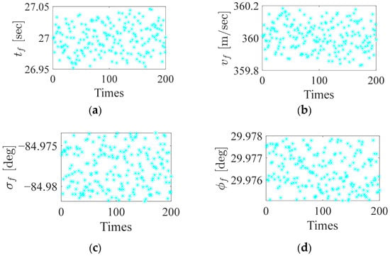
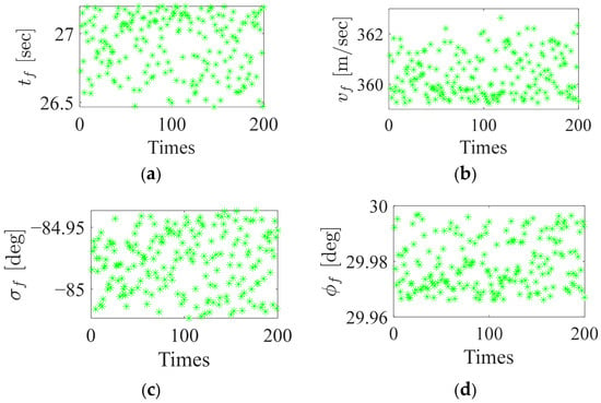
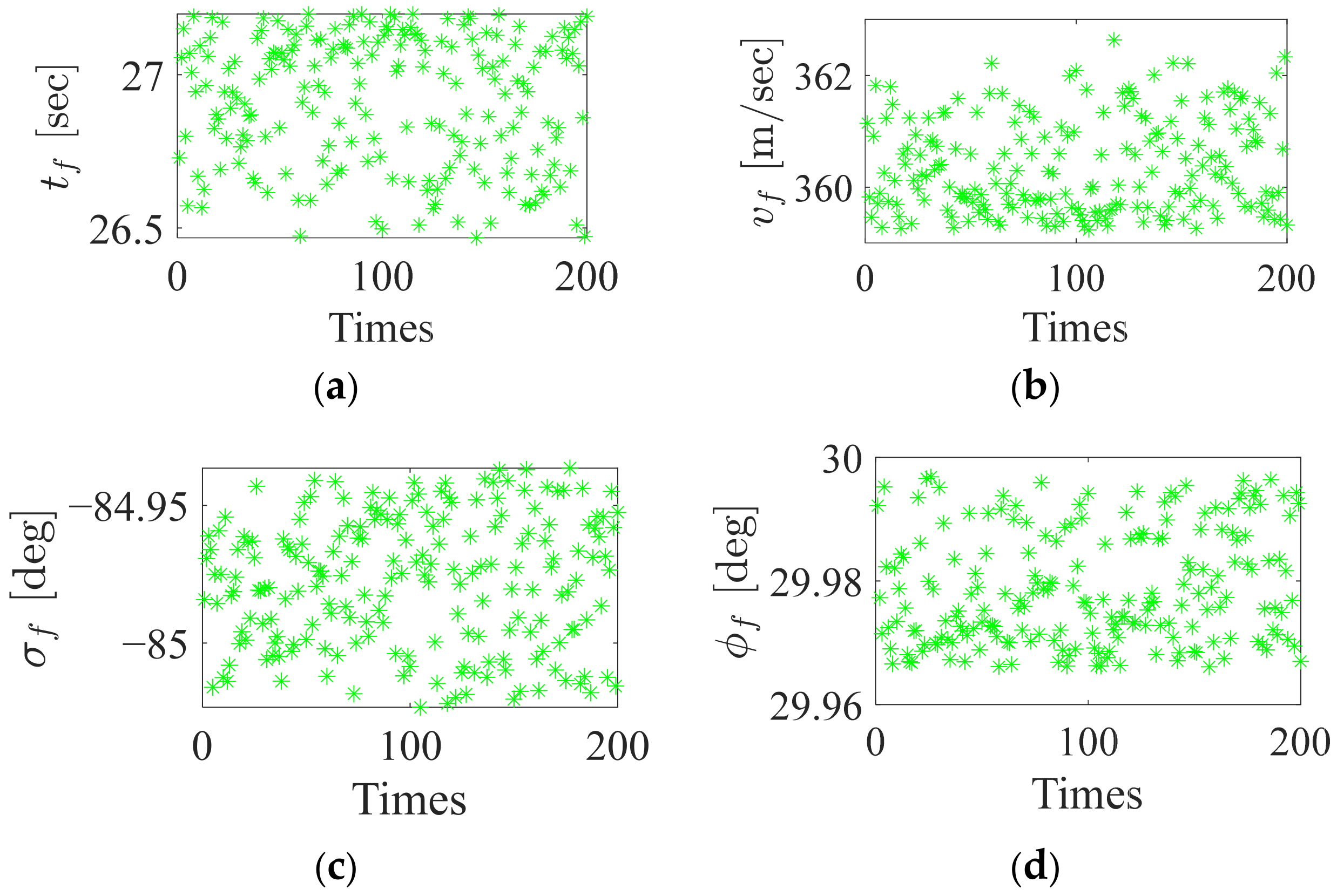
Under the optimized parameters, the normal accelerations $a^{\sigma }$ and $a^{\phi }$ are calculated using the guidance law (18). Deviations in missile mass, lift coefficient, and side-force coefficient may cause the actual normal accelerations to differ from the calculated values. Two scenarios are considered here: (1) simultaneous perturbations within ±5% are applied to $a^{\sigma }$ and $a^{\phi }$, and (2) simultaneous perturbations within ±50% are applied to $a^{\sigma }$ and $a^{\phi }$. The specific implementation process is as follows: In each simulation run, two random numbers are generated within either (0.95, 1.05) or (0.5, 1.5). These numbers are multiplied by the calculated values of $a^{\sigma }$ and $a^{\phi }$, respectively. The resulting values are used as the actual maneuver accelerations applied to the missile. Each scenario is simulated 200 times, and the Monte Carlo simulation results of the relevant variables are shown in Figure 6 and Figure 7.

Figure 6. Monte Carlo results with simultaneous perturbations within ±5% in $a^{\sigma }$ and $a^{\phi }$: (a) impact time $t_f$; (b) impact speed $v_f$; (c) impact angle ${\sigma }_f$; (d) impact angle ${\phi }_f.$

Figure 7. Monte Carlo results with simultaneous perturbations within ±50% in $a^{\sigma }$ and $a^{\phi }$: (a) impact time $t_f$; (b) impact speed $v_f;$ (c) impact angle ${\sigma }_f$; (d) impact angle ${\phi }_f.$

The missile successfully hit the target in all 200 trials at both perturbation levels. These results show that the proposed method performs effectively under the simulation scenario and acceleration-perturbation model considered in this study. Figure 6c,d and Figure 7c,d show that perturbations in $a^{\sigma }$ and $a^{\phi }$ do not affect the accuracy of the impact angles. This is because the impact angles mainly depend on the bias terms. Perturbations in the normal accelerations $a^{\sigma }$ and $a^{\phi }$ are equivalent to perturbations in the bias-term parameters $l^{\sigma }$ and $l^{\phi }$. Therefore, they do not significantly affect the impact angles. However, Figure 6a,b and Figure 7a,b show that these perturbations affect both the impact time and impact speed. For the ±5% perturbation case, the impact time range is (27 − 0.05, 27 + 0.05), with a maximum relative deviation of less than 0.19%; the impact speed range is (360 − 0.2, 360 + 0.2), with a maximum relative deviation of less than 0.056%. For the ±50% perturbation case, the impact time range is (27 − 0.6, 27 + 0.2), with a maximum relative deviation of approximately 2.2%; the impact speed range is (360 − 1, 360 + 3), with a maximum relative deviation of approximately 0.83%. Therefore, under the considered acceleration perturbations, the impact-time and impact-speed deviations remain within the reported ranges, while the impact angles remain close to their prescribed values.

5. Conclusions

This paper proposes a TLBO-based parameter optimization method for terminal guidance under multiple constraints. The method simultaneously optimizes the initial conditions and guidance-law parameters while maintaining a relatively simple guidance-law structure. The considered constraints include impact time, impact angle, impact speed, normal acceleration magnitude and rate, lead angle, and the seeker blind zone. The simulation results show that the optimized trajectory hits the target while satisfying the prescribed terminal and path constraints. The Monte Carlo results further show that satisfactory target-hitting and terminal-state performance is maintained under the specified normal-acceleration perturbations. These results demonstrate the feasibility of the proposed method under the engagement conditions and uncertainty model considered in this study.

References

- Wang, Y.; Wang, C.; Zhu, B.; Liu, G.; Wang, E.; Guo, L. Secure three-dimensional guidance for target strikes under unknown direction attacks and multiple constraints. IEEE Trans. Aerosp. Electron. Syst. 2025, 61, 6951–6963. [Google Scholar] [CrossRef] [Scilit]
- Wu, F.; Chen, Z.; Shao, X.; Wang, K. Nonlinear optimal guidance with constraints on impact time and impact angle. Automatica 2025, 181, 112500. [Google Scholar] [CrossRef] [Scilit]
- Yi, X.; Wang, C.; Dong, W.; Wang, J.; Deng, F.; Xin, M. Wide-envelope cooperative guidance with constrained field-of-view and varying speed against maneuvering targets. IEEE Trans. Aerosp. Electron. Syst. 2025, 61, 9021–9035. [Google Scholar] [CrossRef] [Scilit]
- Lu, D.; Guo, J.; Jiang, R. Two-stage differential game guidance law with terminal angle and hard acceleration constraints. In Advances in Guidance, Navigation and Control: Proceedings of 2024 International Conference on Guidance, Navigation and Control; Springer: Berlin/Heidelberg, Germany, 2025; Volume 18, pp. 20–29. [Google Scholar]
- Wang, N.; Wang, X.; Li, Y. Three-dimensional adaptive dynamic surface guidance law for missile with terminal angle and field-of-view constraints. ISA Trans. 2024, 154, 113–131. [Google Scholar] [CrossRef] [Scilit]
- Li, Y.; Liu, J.; Shan, J.; Wang, J. Guidance law with terminal velocity constraint for hypersonic morphing vehicle. In Advances in Guidance, Navigation and Control: Proceedings of 2024 International Conference on Guidance, Navigation and Control; Springer: Berlin/Heidelberg, Germany, 2025; Volume 9, pp. 326–335. [Google Scholar]
- Shi, H.; Cheng, Z.; Kuang, M.; Zhu, J.; Yan, X.; Li, X. Four-stage guidance law for impact time and angle control based on the Bezier curve. IEEE Trans. Aerosp. Electron. Syst. 2024, 60, 3766–3778. [Google Scholar] [CrossRef] [Scilit]
- Kong, X.; Zhang, C. Parameter optimization method for predictor–corrector guidance with impact angle constraint. Int. J. Aerosp. Eng. 2024, 2024, 4540925. [Google Scholar] [CrossRef] [Scilit]
- Duan, X.; Wang, J.; Wang, Y.; Fan, S. Initial-condition-aware polynomial guidance with impact time and angle constraints. Aerospace 2025, 12, 484. [Google Scholar] [CrossRef] [Scilit]
- Rao, R.V.; Savsani, V.J.; Vakharia, D.P. Teaching–learning-based optimization: A novel method for constrained mechanical design optimization problems. Comput.-Aided Des. 2011, 43, 303–315. [Google Scholar] [CrossRef] [Scilit]
- Qiu, J.; Xiao, S. Multi-objective terminal trajectory optimization based on hybrid genetic algorithm pseudospectral method. Electron. Lett. 2024, 60, e13281. [Google Scholar] [CrossRef] [Scilit]
- Bao, C.; Fan, J.; Ji, Y. A PSO-MLP-based terminal guidance law profile parameter prediction method under field-of-view constraints. In 2025 China Automation Congress (CAC); IEEE: New York, NY, USA, 2025; pp. 3113–3117. [Google Scholar]
- Han, T.; Hu, Q.; Xin, M. Analytical solution of field-of-view limited guidance with constrained impact and capturability analysis. Aerosp. Sci. Technol. 2020, 97, 105586. [Google Scholar] [CrossRef] [Scilit]
- Wang, P.; Lee, C.-H.; Liu, Y.; Tahk, M.J. Nonlinear three-dimensional guidance for impact time and angle control with field-of-view constraint. IEEE Trans. Aerosp. Electron. Syst. 2024, 60, 264–279. [Google Scholar] [CrossRef] [Scilit]
- He, S.; Lee, C.-H.; Shin, H.-S.; Tsourdos, A. Optimal three-dimensional impact time guidance with seeker’s field-of-view constraint. Chin. J. Aeronaut. 2021, 34, 240–251. [Google Scholar] [CrossRef] [Scilit]
- Duvvuru, R.; Maity, A.; Umakant, J. Three-dimensional field of view and impact angle constrained guidance with terminal speed maximization. Aerosp. Sci. Technol. 2022, 126, 107552. [Google Scholar] [CrossRef] [Scilit]
- Kim, H.-G.; Lee, J.-Y. Generalized guidance formulation for impact angle interception with physical constraints. Aerospace 2021, 8, 307. [Google Scholar] [CrossRef] [Scilit]
- Zhou, G.; Xia, Q. A guidance strategy for strapdown seeker considering minimum field-of-view angle constraint. Int. J. Aerosp. Eng. 2020, 2020, 5247257. [Google Scholar] [CrossRef] [Scilit]
- Chen, K.-Y.; Lee, Y.-L.; Liao, S.-J.; Kung, C.-C. The design of particle swarm optimization guidance using a line-of-sight evaluation method. Comput. Electr. Eng. 2016, 54, 159–169. [Google Scholar] [CrossRef] [Scilit]
Disclaimer/Publisher’s Note: The statements, opinions and data contained in all publications are solely those of the individual author(s) and contributor(s) and not of MDPI and/or the editor(s). MDPI and/or the editor(s) disclaim responsibility for any injury to people or property resulting from any ideas, methods, instructions or products referred to in the content. |
© 2026 by the authors. Licensee MDPI, Basel, Switzerland. This article is an open access article distributed under the terms and conditions of the Creative Commons Attribution (CC BY) license.