


Abstract
This paper proposes a novel elasto-geometrical coupling calibration and an adaptive parameter identification method for flexible redundant manipulators. For the modeling, an elasto-geometrical coupling calibration model containing kinematic parameter errors and non-kinematic errors is constructed. Secondly, an adaptive identification rule is formulated to suppress the elasto-geometrical modeling errors according to the residual linearization errors in each iteration, thus obtaining accurate identification results even in the case of highly elastic joints. Thirdly, a dual-target measuring strategy based on multi-source sensing is designed to obtain high-precision hand-eye data; thus, lightweight sensors and a vision system suitable for flexible light-load manipulators can be practically used for the calibration. As revealed by simulation tests, the newly developed identification algorithm can progressively compensate for considerable linearization modeling discrepancies for a redundant robotic arm with 12 highly elastic joints. All error parameters are estimated with an accuracy above 99% through iterative updates. Corresponding experiments are carried out on an eight-joint cable-driven elastic redundant manipulator, and the results indicate the new calibration method reaches the fastest algorithm convergence and residuals at the same level when compared with two traditional ones.
1. Introduction
Absolute positioning accuracy is a decisive performance metric for robotic manipulators, which largely governs the execution quality of robot arms in real-world applications [1]. For conventional industrial manipulators, kinematic parameter errors constitute the primary source of absolute positioning deviation. These errors mainly stem from imperfections introduced in the manufacturing, assembly, and transmission phases of robot links and joints [1,2]. Traditional calibration approaches can effectively compensate such kinematic parameter deviations and boost the absolute positioning performance of industrial robots, thereby satisfying accuracy requirements for most routine industrial assignments [1,2]. Nevertheless, typical industrial manipulators possess high structural stiffness, relatively long link structures and limited degrees of freedom. Such characteristics make them ill-suited for unstructured-environment tasks requiring soft contact with compliant workpieces including diapers and medical pads [3,4]. Against this practical demand, redundant manipulators featuring elastic joints, short links and a large number of joint units have emerged as a promising technical alternative [3,4,5].
A critical drawback of many classic calibration techniques is that they seldom take joint angle errors induced by robot self-weight and external payload into account during the calibration process. Li et al. [6], Chen et al. [7], and Yang et al. [8] established calibration frameworks founded on the product-of-exponentials (POE) theory; however, all kinematic parameters within their models were treated as constant quantities. Jiang et al. [9,10,11] also developed several calibration models, yet these works likewise only adopted fixed kinematic parameters without considering payload-driven joint deviations.
Apart from pure kinematic calibration research, considerable investigations have focused on joint compliance characteristics of robotic systems. A series of studies explored non-kinematic parameter calibration by exploiting link mass-distribution information. Nubiola and Bonev, together with their collaborators [12,13,14,15], constructed integrated models incorporating both kinematic and non-kinematic error terms, while Klimchik et al. [16] carried out parameter identification work for manipulator stiffness models under real industrial conditions. Gong et al. [17] formulated non-kinematic errors with gravitational and center-of-mass variables that are hard to acquire by direct measurement, circumventing the need for explicit identification of these hard-to-measure physical quantities. Some other studies targeted non-kinematic errors originating from external loads. Chen and Kao [18] built a complete stiffness transformation from joint space to Cartesian space via the conservative congruence transformation (CCT), which supports calibration under external loading conditions. On this basis, Dumas et al. [19] simplified the stiffness model to facilitate efficient stiffness identification while retaining acceptable accuracy. Zhou et al. [20] further proposed a unified framework that simultaneously considers geometric inaccuracies and compliance-related non-kinematic parameters. To improve parameter identifiability amid practical measurement noise, Mamedov et al. [21] derived simplified model variants by evaluating parameter scaling and noise influences. Theissen et al. [22] presented an elastostatic calibration scheme that employs external loads of diverse directions and magnitudes. Du et al. [23] and Chen et al. [24] further built functional mappings that connect two categories of non-kinematic parameters to end-effector positioning errors.
Although diverse calibration models have been developed, research regarding parameter identification for elasto-geometrical coupled redundant manipulators remains limited. One widely-adopted strategy is payload-invariant iterative identification. Under this paradigm, error parameters solved in the prior iteration are incorporated into the calibration model for subsequent computation of a new set of error parameters. The iteration proceeds until the magnitude of solved error parameters drops below the preset threshold, and the final error-parameter solution is accumulated from results of all iterative cycles [7,15,25]. Besides this cumulative iterative scheme, scholars have put forward identification algorithms built upon the Levenberg–Marquardt approach, which adaptively modifies the damping factor at each iteration. The damping factor multiplied by the identity matrix is added to the Jacobian matrix of the least-squares formulation, ensuring positive-definite property throughout numerical iterations [26].
Nevertheless, state-of-the-art elasto-geometrical coupling modeling and parameter calibration methods for redundant robotic arms still have some limitations. First, most existing calibration models are originally designed for high-rigidity, low-degree-of-freedom industrial robots with high assembly precision. These models only account for partial kinematic errors while neglecting the coupled effects of non-kinematic errors, thus exhibiting poor adaptability to flexible redundant manipulators with multiple joints and high structural flexibility. Second, traditional identification algorithms employ uniform and fixed iteration criteria throughout the calibration process. When coping with high-dimensional model problems accompanied by significant linearization errors, such generic iteration strategies are susceptible to severe linearization error interference, leading to degraded convergence stability and even numerical divergence. Third, prevailing calibration schemes mostly rely on bulky and heavy sensing devices, which are incompatible with the light-load characteristic of flexible manipulators. Although lightweight target sensors can match the light-load operational features, they suffer from inherent drawbacks such as inaccurate hand-eye calibration and low measurement precision. The inherent contradiction between sensor structural adaptability and measurement accuracy substantially impedes the implementation of robust calibration schemes, which severely restricts the practical applicability of calibration for flexible redundant manipulators calibration.
For this purpose, three main contributions are presented in this work: (1) An elasto-geometric coupling calibration model is constructed that incorporates both kinematic parameter deviations and non-kinematic errors, which improves the model’s integrity and generalization capability. (2) An adaptive parameter updating law is formulated to progressively alleviate the adverse effects introduced by linearization errors. (3) A dual-target relative pose measurement scheme relying on multi-source sensing is proposed to obtain high-precision hand–eye measurements of the manipulator. Based on this, a lightweight calibration scheme applicable to flexible light-load manipulators is proposed.
The structure of this paper is outlined as follows. Section 2 constructs the elasto-geometrical error model as well as the corresponding calibration model. Section 3 develops an iterative parameter identification algorithm. In Section 4, numerical simulations are carried out on a 12-joint elastic robotic manipulator to verify both the convergence property of the proposed identification algorithm and the precision of its solved parameter results. Section 5 presents experimental tests implemented on an eight-joint cable-driven manipulator, which further validates the prediction accuracy of the newly-derived calibration model and the practical effectiveness of the identification algorithm. Finally, Section 6 summarizes the main conclusions of this work.
2. Kinematic Error Model with Rigid–Flexible Coupling
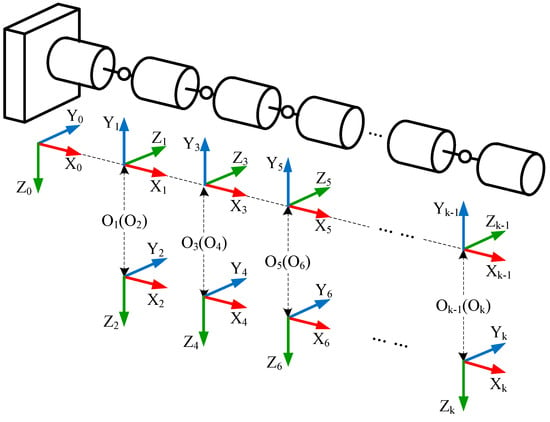
Figure 1 illustrates the joint coordinate systems of a k-degree-of-freedom serial hyper-redundant manipulator, which are defined following the modified Denavit–Hartenberg (MDH) notation.
Figure 1.
Coordinate frames of a hyper-redundant manipulator with k joints.
Let F0 and Fi (i = 1,2, …,k) denote the base frame and the joint coordinate frames of the hyper-redundant manipulator, respectively. The forward kinematic model of joint i is then given by
where i−1Ti is the nominal transformation matrix from Fi−1 to Fi, expressed as
In the above equation, Rx(*) and Rz(*) represent transformations around the X and Z axes of the joint coordinate frame, respectively, while Dx(*) and Dz(*) represent translations along these axes. The nominal MDH parameters of joint i are αi, ai, θi, and di, where αi, ai, and di are fixed structural parameters, and θi is the commanded rotation angle of joint i at the jth measurement configuration. The MDH parameter errors of joint i are represented by Δui = [δαi, δai, δθi, δdi]T. Based on differential transformation theory, the matrix Ci mapping Δui to the pose error of Fi is given by
In the matrix elements of Equation (3), S and C are shorthand for the trigonometric functions sin(*) and cos(*), respectively.
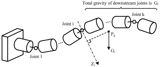
The effect of the manipulator’s self-weight on the joint rotation angle θi is considered next. First, the gravitational torque acting on joint i must be calculated. As shown in Figure 2, calculating this torque, MGi, requires the total gravitational force Gi of all downstream joints (joints i through k) and its moment arm relative to the axis Zi.
Figure 2.
Total gravitational force Gi of the downstream joints of joint i and its moment arm relative to the axis Zi.
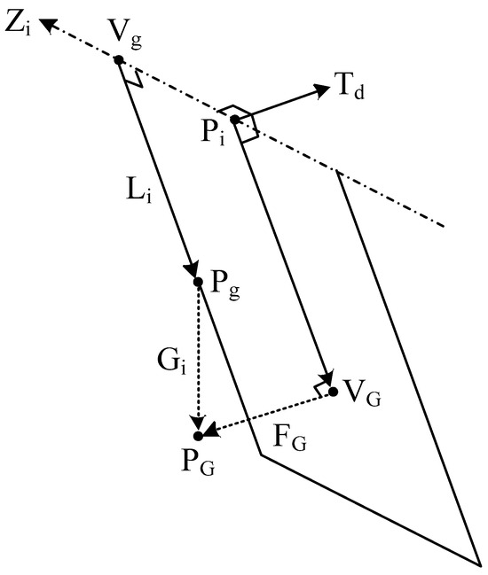
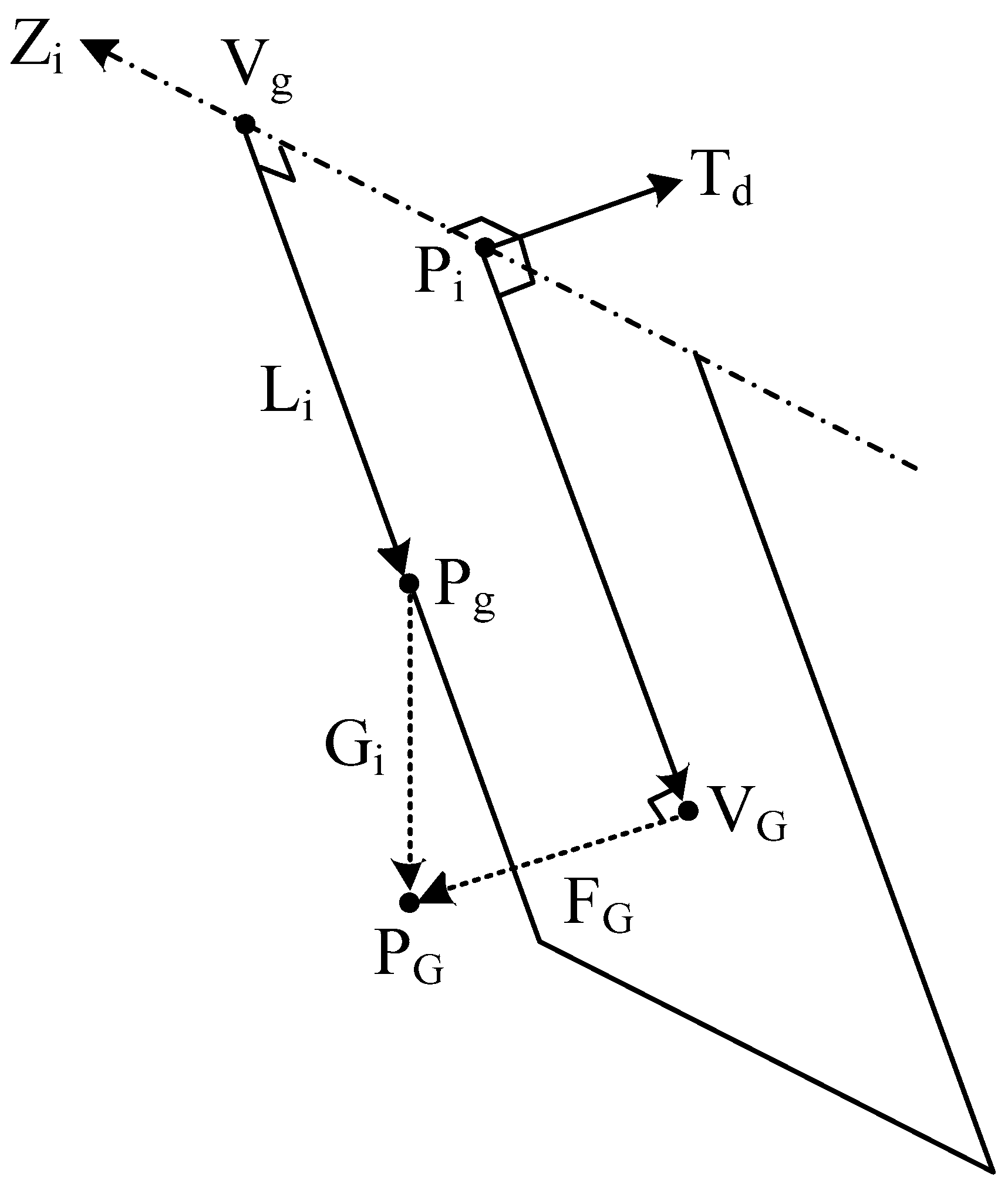
As shown in Figure 3, let Zi = [Zix, Ziy, Ziz]T denote the direction vector of the axis of joint i, comprising the first three elements of the third column of 0Ti obtained from Equation (1). The joint center, i.e., the origin of Fi, is Pi = [Pix, Piy, Piz]T, comprising the first three elements of the fourth column of 0Ti. The combined center of mass of all its downstream joints is denoted by Pg = [Pgx, Pgy, Pgz]T.
Figure 3.
Moment arm Li of the total gravitational force Gi and the force component FGi perpendicular to Li.
Calculating the combined center of mass Pg of all downstream joints of joint i requires the center-of-mass positions Pgs and Pgi. Here, Pgs is the combined center of mass of the terminal joint k and its mounted sensor, while Pgi represents the center-of-mass position of the remaining downstream joints. Since the joints and the terminal sensor generally have axisymmetric structures, Pgs can be specified by the distance dgs from Ok to the center of mass along Xk. Similarly, Pgi can be specified by the distance dgi from the joint-frame origin Oi to the center of mass along Xi. Thus, the coordinates of Pgs in F0 are calculated as
The coordinates of the center of mass Pgi in F0 are calculated as
The three coordinates of the combined center of mass Pg of all downstream joints of joint i, including the terminal sensor, are calculated as
where the symbols “(1)”, “(2)”, and “(3)” denote the first, second, and third elements of a vector, respectively, and avg(*) denotes the averaging operation.
The foot of the perpendicular from Pg to the axis Zi, denoted by Vg, can then be expressed as
where t is a scalar. The moment-arm vector Li is defined as
Since Li must be perpendicular to Zi, t is obtained as
Substituting the above expression into Equation (7) yields Vg = [Vgx, Vgy, Vgz]T, after which the moment-arm vector Li can be calculated using Equation (8).
Given the total mass ms of the terminal sensor and the mass mi of each joint, the total gravitational force Gi of all downstream joints of joint i is given by
In Equation (10), g is the gravitational acceleration. Expressing Gi in the base frame F0 as the vector Gg = [0, 0, −Gi]T gives the coordinates of the endpoint of this vector as
Define Td = [Tdx, Tdy, Tdz]T as the normal vector to the plane containing Li and Zi, and let VG = [VGx, VGy, VGz]T be the projection of PG onto this plane. Since the vector PiVG is perpendicular to Td, and the vector VGPG is perpendicular to both Zi and Li, the following system of equations can be established:
Solving the system in Equation (12) yields the projection point VG. Its analytical solution is given in Appendix A. The component vector of Gi that is perpendicular to both the moment-arm vector Li and the joint axis Zi is then given by
And the explicit solution of FGi is also given in Appendix A. If the angle between Td and Gg is less than 90°, the gravitational torque acting on joint i is given by
If the angle between Td and Gg is greater than or equal to 90°, the gravitational torque acting on joint i is given by
The additional rotation angle δθiG of joint i induced by the gravitational torque can be expressed as
Suppose that the measured actual pose of the sensor frame mounted on joint k at the jth measurement configuration {θ1, …, θk}j is (0Tsa)j. Combining this pose with the transformation matrix kTs from the frame of joint k to the sensor frame gives (0Tka)j = [(0Tsa)j]−1kTs. The elements of (0Tka)j are denoted as follows:
Using the elements of (0Tka)j in Equation (17), the corresponding actual pose vector pka(j) can be calculated as
where atan2(y, x) is the two-argument arctangent function.
Equation (1) gives the nominal transformation matrix (0Tk)j of joint k at the configuration {θ1, …, θk}j. The elements of (0Tk)j are denoted as follows:
The corresponding nominal pose vector pk(j) can then be obtained from (0Tk)j as
The pose-error vector Ej of joint k at the measurement configuration {θ1, …, θk}j is consequently obtained as
Combining all λi and all Δui into a single vector gives
The mapping from Δu to Ej at the jth measurement configuration used for calibration can then be established as
In Equation (23),
In Equation (24),
In Equation (25),
In Equation (26),
The matrix elements in Equations (28) and (29) are obtained from the forward kinematic equation
If a total of n measurement configurations (j = 1,2,…,n) are used for calibration, Equation (23) can be extended to
In Equation (31),
Equation (31) is rearranged as follows to solve for Δu:
In Equation (33), J+ denotes the generalized inverse of J.
3. Asymptotic Iterative Identification Algorithm
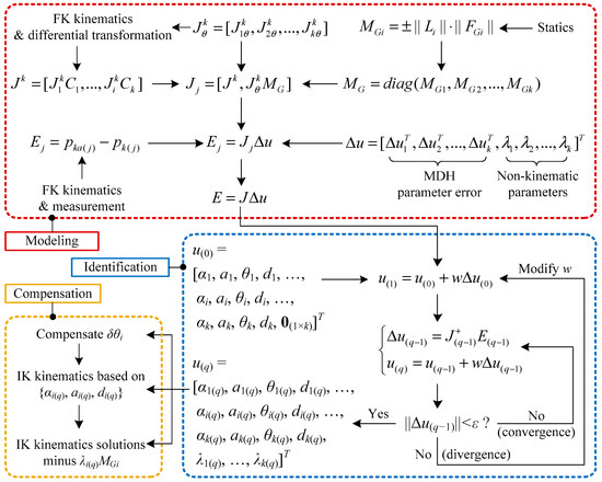
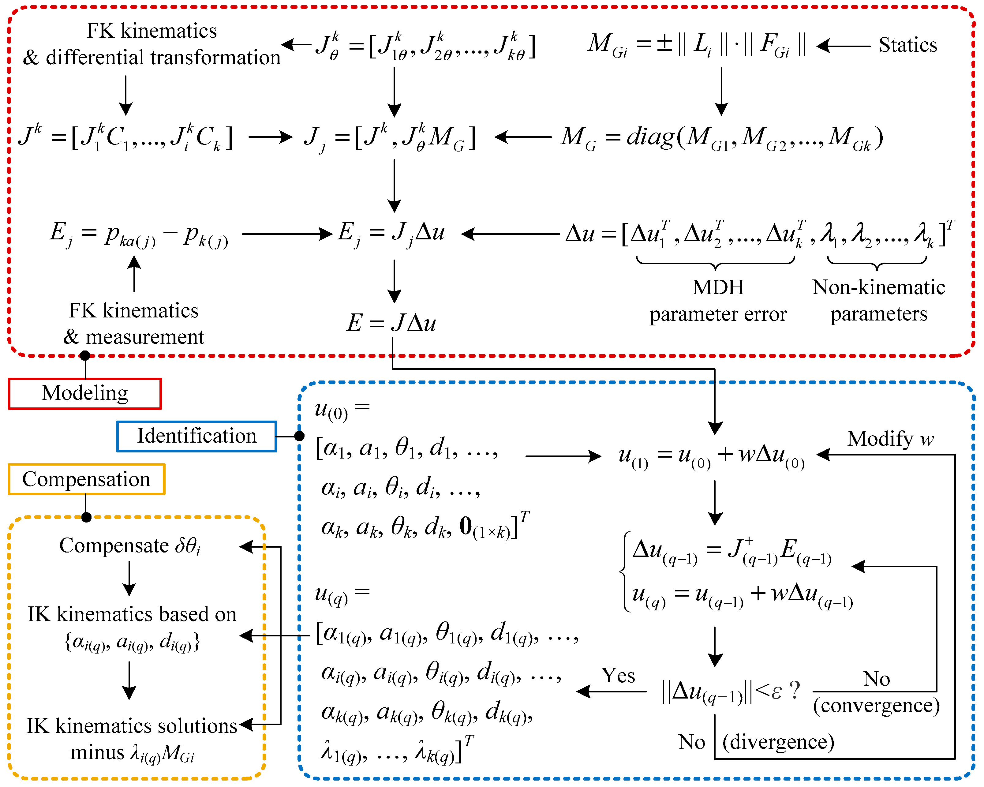
The workflow of the calibration method is shown in Figure 4. The modeling procedure has been described in detail in Section 2, while the identification and compensation procedures are shown in the “adaptive iterative identification” and “classified compensation” modules of Figure 4, respectively.
Figure 4.
Flowchart of the calibration method.
Let u(0) = [α1, a1, θ1, d1, …, αi, ai, θi, di, …, αk, ak, θk, dk, 0(1×k)]T denote the vector of nominal MDH parameters and joint elastic coefficients of the manipulator at the jth measurement configuration, where {θ1, θ2, …, θk} are the commanded joint rotation angles at this configuration. The MDH parameters used to establish Equation (33) are therefore elements 1 through 4k of u(0). The value of Δu first obtained from Equation (33) is defined as the initial identification result, Δu(0) = [δα1(0), δa1(0), δθ1(0), δd1(0), …, δαi(0), δai (0), δθi (0), δdi (0), …, δαk(0), δak(0), δθk(0), δdk(0), λ1(0), …, λk(0)]T, where the subscript “(0)” denotes the initial identification. According to the following equation, Δu0 is multiplied by the weight w and then added to u(0) to obtain u(1):
The weight w is selected manually and generally satisfies w ≤ 1.
The vector u(1) = [α1(1), a1(1), θ1(1), d1(1), …, αi(1), ai(1), θi(1), di(1), …, αk(1), ak(1), θk(1), dk(1), λ1(1), …, λk(1)]T, obtained from Equation (34), replaces u(0) used in Equation (34). Equation (33) is then reconstructed to obtain the first iterative identification result, Δu(1), with u(1) serving as the nominal parameter vector. The subscript “(1)” denotes the first iterative identification. Specifically, {αi, ai, di} are replaced by {αi(1), ai(1), di(1)} from u(1), while θi is replaced by θi(1)+λi(1)MGi. Here, MGi is the gravitational torque acting on joint i at the measurement configuration {θ1, θ2, …, θk}j, calculated using Equation (14) or (15).
Since the above steps must be repeated, Equations (33) and (34) are generalized as follows:
The subscripts “(q−1)” and “(q)” denote the (q − 1)th and qth iterative identifications, respectively. An increasing trend in the norm ||Δu(q−1)|| obtained iteratively from Equation (35) indicates divergence. In this case, the weight w in Equation (34) is reduced to decrease the linearization error at each iteration, and the iteration is restarted from q = 1. A decreasing trend in ||Δu(q−1)|| indicates convergence, and the iteration stops when ||Δu(q−1)|| < ε. Here, ε is a threshold selected according to the required calibration accuracy. The resulting vector u(q) = [α1(q), a1(q), θ1(q), d1(q), …, αi(q), ai(q), θi(q), di(q), …, α12(q), a12(q), θ12(q), d12(q), λ1(q), …, λkq)]T contains the final identified MDH parameters and joint elastic coefficients.
Compensation for the MDH parameter errors and joint elastic coefficients is performed in three substeps. First, for i = 1, …, k, the (4i − 1)th element δθi of u(q) − u(0) at any measurement configuration is taken as the zero-offset error of joint i, and all δθi are compensated simultaneously in the control system. Next, {αi(q), ai(q), di(q)} from u(q) are used as the nominal MDH parameters of the manipulator to solve the inverse kinematics. Finally, for i = 1, …, k, λi(q)MGi is subtracted from the rotation-angle command for joint i obtained from the inverse kinematic solution, yielding the final compensated rotation-angle commands for all joints.
4. Simulation
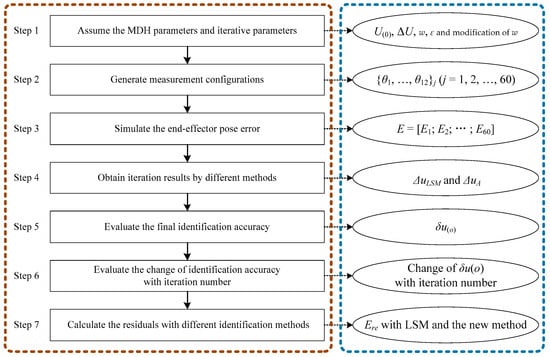
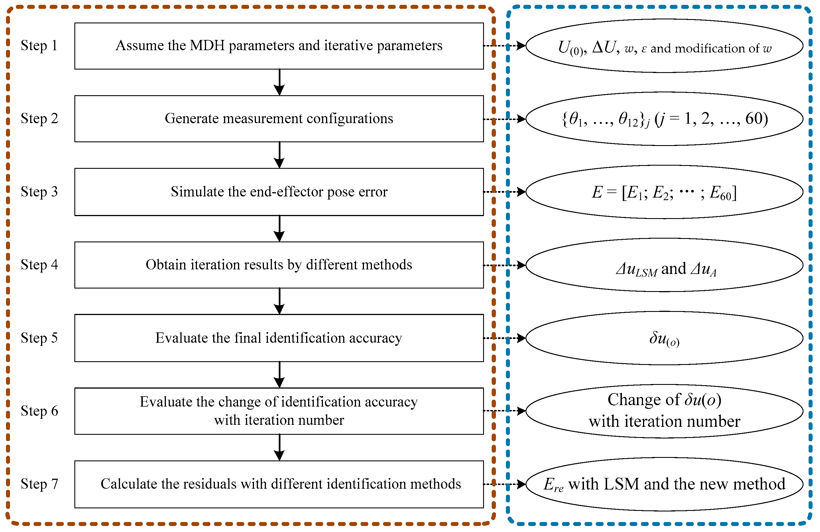
The simulation uses the proposed model with rigid–flexible coupling. The error parameters are identified using the adaptive iterative identification algorithm and a conventional iterative least-squares identification algorithm with a fixed weight, and their convergence rates and accuracies are compared. The identification algorithm is performed on MATLAB (R2023b, 2.10 GHz CPU) in both the simulation and experiment. As shown in Figure 5, the simulation is performed in the following steps.
Figure 5.
Flowchart of simulation.
Step 1: The nominal MDH parameters of the hyper-redundant manipulator are assumed to be those listed in Table 1, while the MDH parameter errors and joint elastic coefficients are given in Table 2 (k = 12). The initial iteration weight is w = 1, and the threshold is ε = 0.02. Whenever the iteration diverges, w is reduced by multiplying it by 0.1.
Table 1.
Nominal MDH parameters of the redundant manipulator.
Table 2.
MDH parameter errors and joint elastic coefficients of the hyper-redundant manipulator.
Step 2: The measurement configurations {θ1, …, θ12}j (j = 1, 2, …, 60) are selected using the DETMAX algorithm.
Step 3: The vector E required for calibration is generated by simulation using Equations (17)–(21). The measurement noises need to be simulated. According to the real experimental setup in Section 5, the positional measurement accuracies of the camera and the laser tracker are assumed to be 0.15mm and 0.03mm, respectively. Marker-1 and marker-2 are both 50mm × 50mm in size. Thus, the measurement uncertainty distributions can be roughly set as ~N [0,(0.18mm/3)2] for the positional part and ~N [0,(0.0036rad/3)2] for E, respectively. Accordingly, 103 sets of the measurement noises are generated and added to the pose vector E in Equation (31).
Step 4: The conventional least-squares identification algorithm [7] and the proposed adaptive iterative identification algorithm are used to solve for Δu based on Equation (33). The corresponding results are denoted by ΔuLSM and ΔuA, respectively.
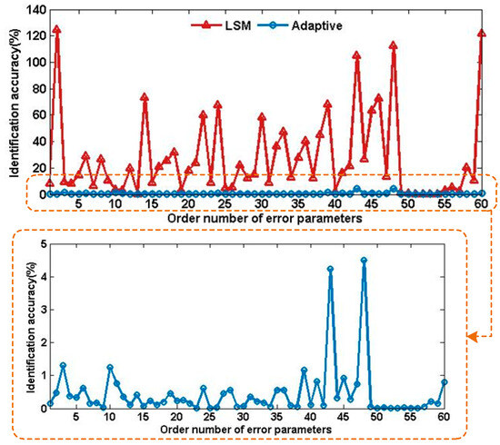
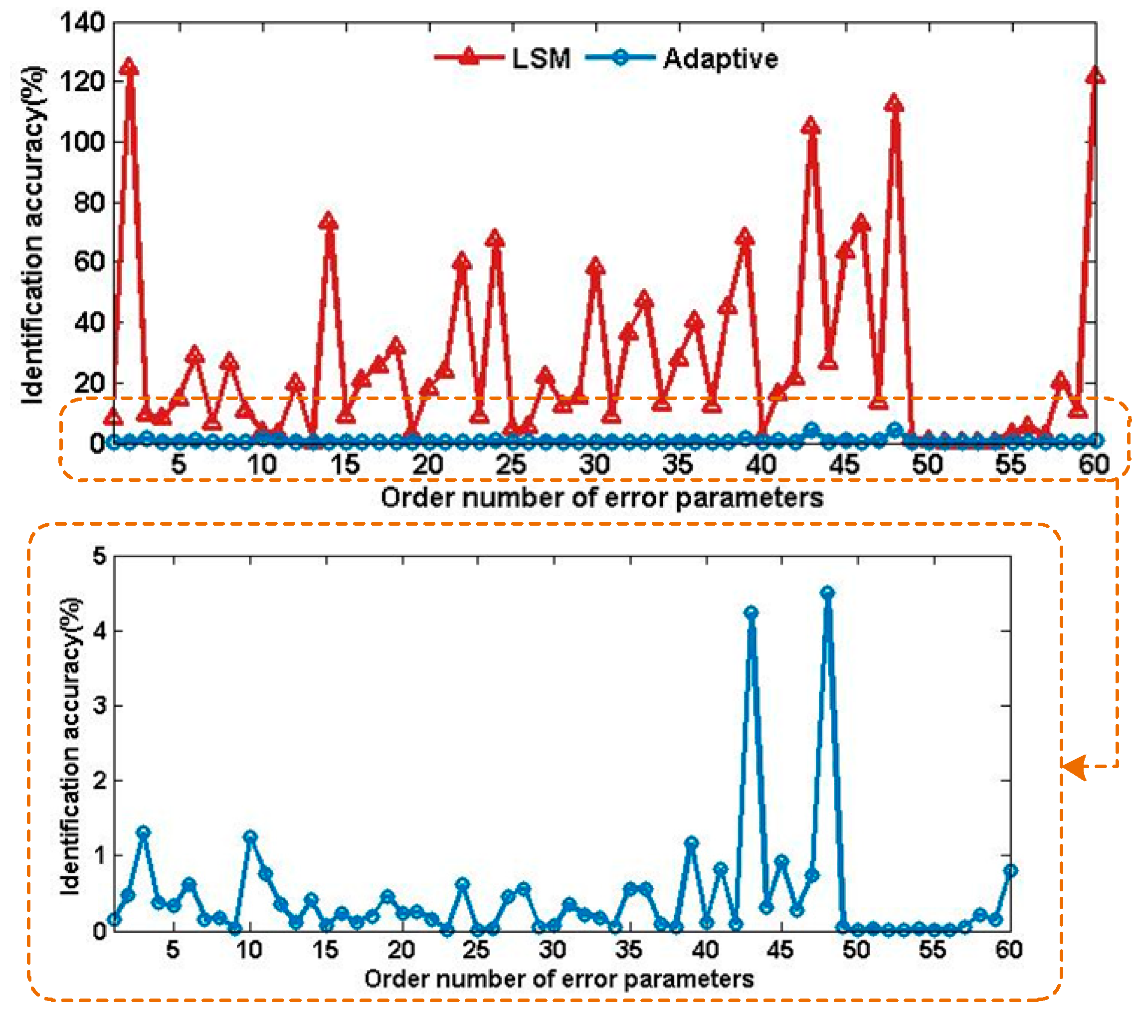
Step 5: The identification accuracy of the oth element in each of ΔuLSM and ΔuA is denoted by δu(o) and calculated using the following equation. Here, o is the index of an error parameter in Δu; the elements δα1, δa1, …, λ12 in both ΔuLSM and ΔuA are indexed sequentially by o = 1, 2, …, 60.
Here, Δuca(o) is the identified result corresponding to the assumed value Δu(o). Figure 6 shows the identification accuracies δu(o) for ΔuLSM and ΔuA.
Figure 6.
Identification accuracy comparison between the different methods in simulation.
As reflected in Figure 6, the identification accuracy indices δu(o) of the presented method achieve values superior to 5% upon convergence. In comparison, the least-squares method yields highly unreliable estimates for certain parameters, whose errors go beyond 120%.
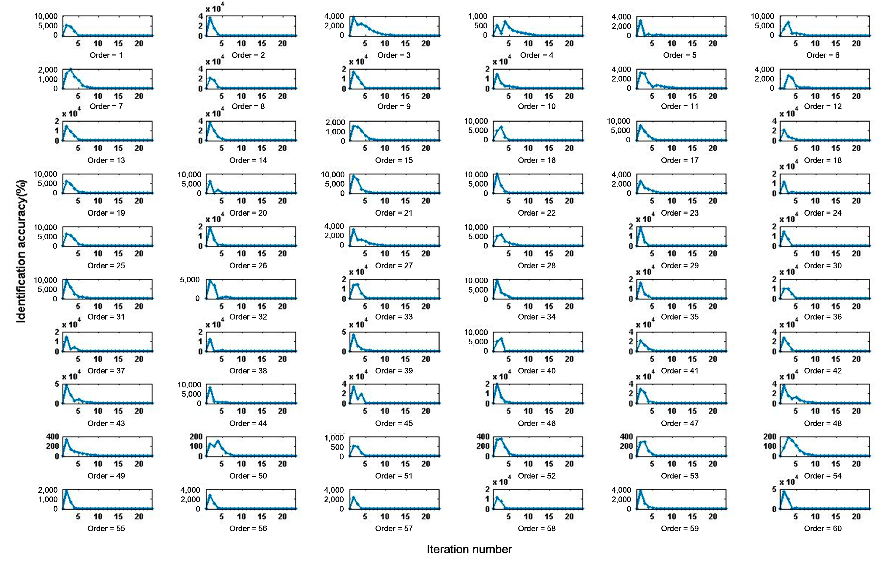
Step 6: For the proposed method, Equation (36) is used to evaluate the identification accuracy δu(o) of each parameter as a function of the number of iterations. The results are shown in Figure 7.
Figure 7.
Trend in identification accuracy of each error parameter with iteration number in simulation.
As illustrated in Figure 7, the δu(o) values of individual error parameters keep reducing along with growing iteration numbers and eventually settle at a small constant level. One or multiple inflection points can be observed on some curves: before convergence, the residuals stop decreasing and even grow. This phenomenon arises because the absolute values of linearization errors for individual parameters are not guaranteed to decrease at each iteration step. Benefiting from the adaptive weighting strategy of the identification method, δu(o) can quickly revert to a downward trend and converge successfully.
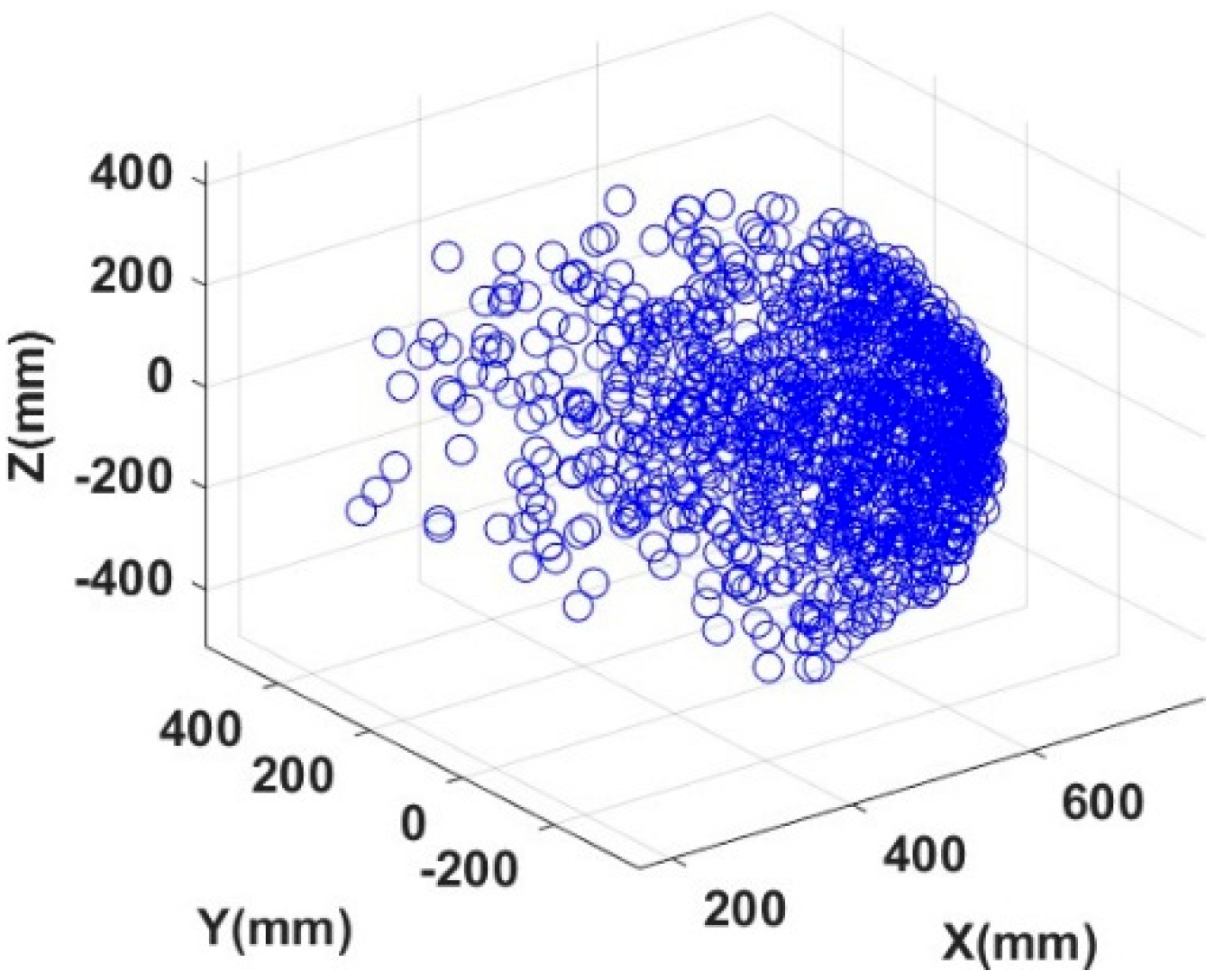
Step 7: A total of 1000 measurement points are randomly generated within the manipulator’s workspace. Their distribution is shown in Figure 8.
Figure 8.
Distribution of test points.
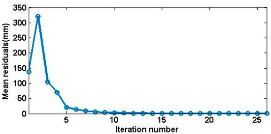
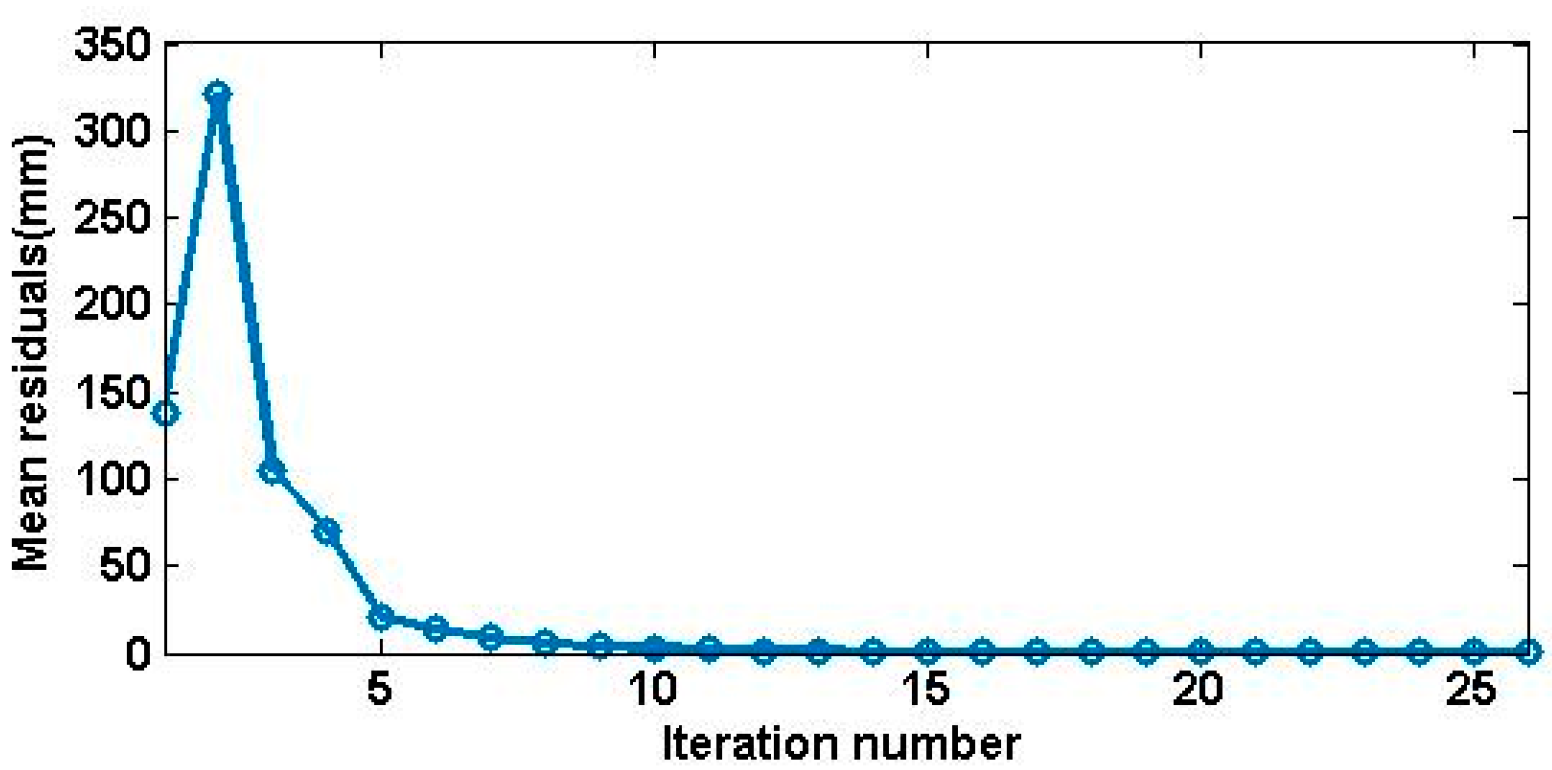
Error compensation is performed using the identification result ΔuA from each iteration. The positioning residual Ere of joint 12 at the testth measurement point (test = 1, 2, …, 1000) is calculated using Equation (37). In Equation (37), Δxtest, Δytest, and Δztest are the corresponding components of E obtained in Step 3. The results are shown in Figure 9.
Figure 9.
Trend in mean residual with iteration number in simulation.
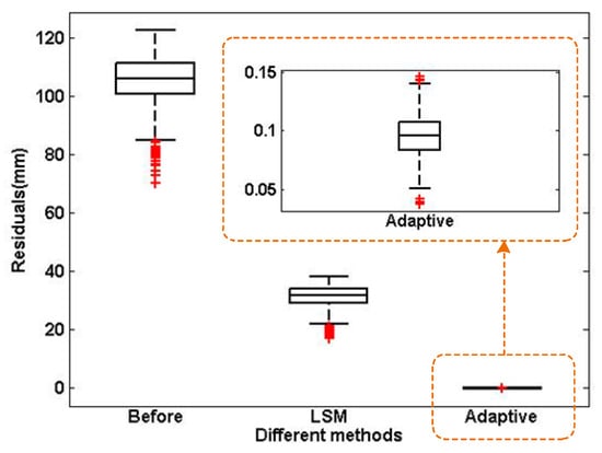
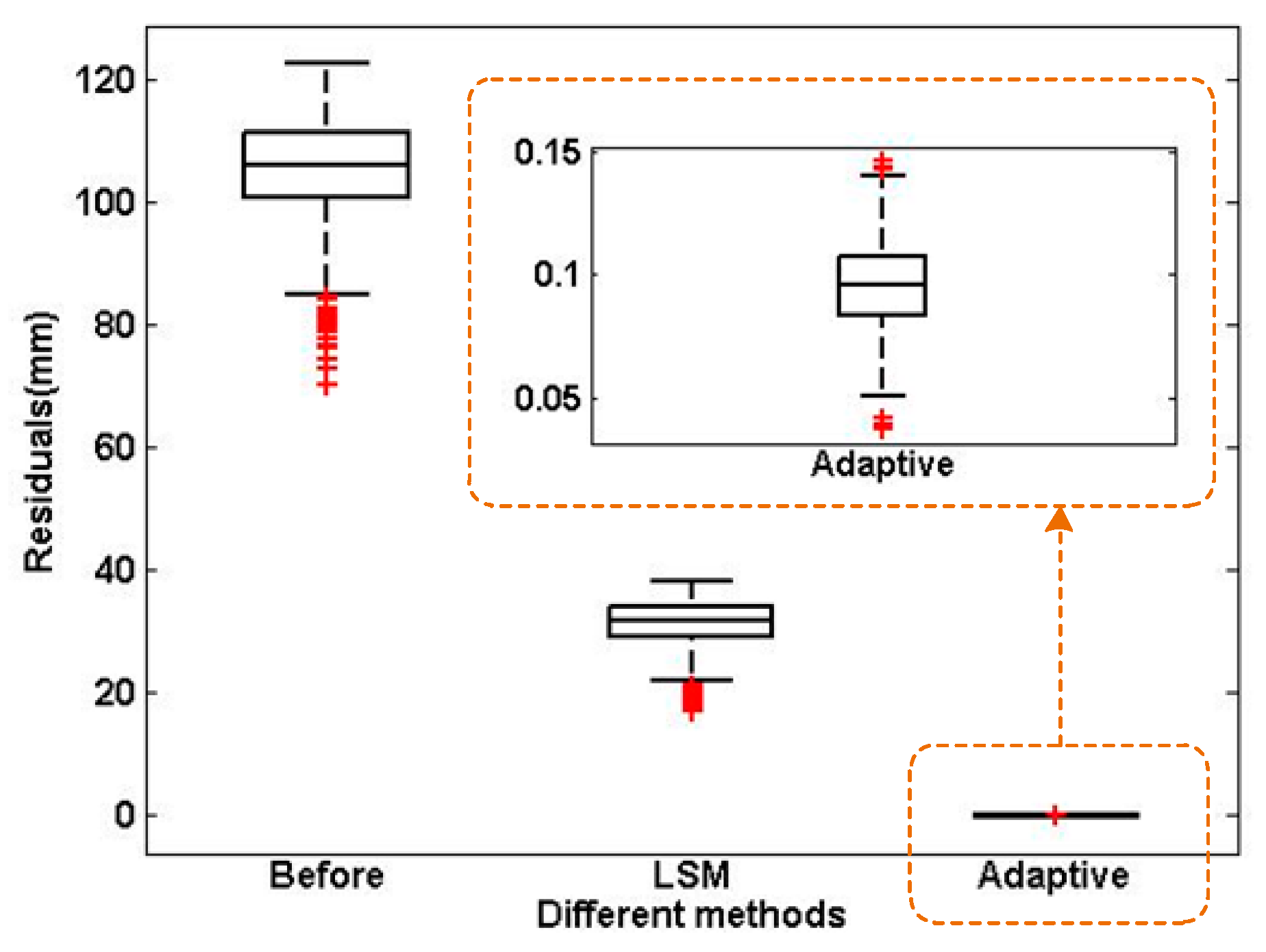
Consistent with the trend in Figure 8, Figure 9 shows that the positioning residuals gradually decrease with the increase in the number of iterations and finally stabilize, although fluctuations occur during the initial iterations. Error compensation is then performed using the final identification results ΔuLSM and ΔuA, respectively, and Equation (37) is used to calculate the absolute positioning residual Ere of joint 12. Meanwhile, Step 3 and Equation (37) are used to obtain the positioning error of the uncalibrated manipulator at measurement point test, which serves as the baseline for comparison with the two sets of residuals. The statistical results for the three groups are shown in Figure 10.
Figure 10.
Comparison of residuals for different methods in simulation.
As plotted in Figure 10, the median residual values obtained by the LSM and the newly developed algorithm reach 31.524 mm and 0.095 mm separately. The proposed strategy attains the minimal residual and lifts the calibration accuracy to roughly 99.7%. The overall experimental outcomes reveal that it can provide a generalized description for non-kinematic errors and enrich the calibration model, allowing more faithful depiction of the rigid–flexible coupling features of the robotic arm. In addition, the iterative identification scheme mitigates the rise in linearization errors originating from non-kinematic parameters and maintains the identification accuracy of unknown parameters.
5. Experiment
5.1. Experimental Setup
Experiments are conducted on a cable-driven redundant manipulator. The manipulator has eight joints alternating between pitch and yaw, with eight DoFs in total. The length of each manipulator link is 110 mm, with a total reach of 440 mm. Each joint is driven by two cables for bidirectional rotation, and each cable is actuated by an independent motor to regulate its retraction and release. A vision system is adopted for pose measurement. The experiment is conducted at a room temperature of 25 °C. The nominal kinematic parameters of the robot are summarized in Table 3, and the principal specifications of the lens and industrial camera are given in Table 4. This platform is used to evaluate parameter identification and the resulting improvement in absolute positioning accuracy.
Table 3.
Nominal kinematic parameters in experiment.
Table 4.
The main specifications of the vision system.
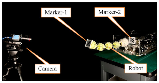
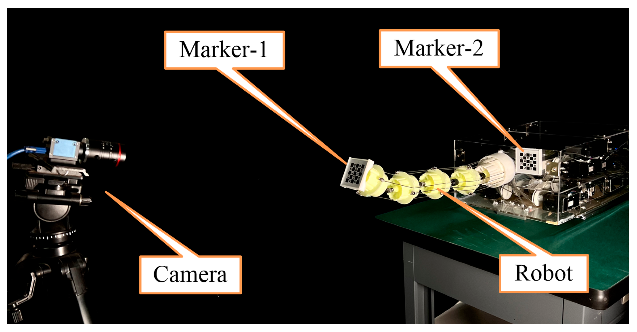
As shown in Figure 11, marker-1, measuring 50 mm × 50 mm, is attached near the robot tip, while marker-2 of the same size is fixed near the base. The camera is positioned to observe marker-1 throughout the selected measurement configurations. The visibility of the markers and the quality of their images should be considered during the configuration selection.
Figure 11.
Installation of sensors and instruments for calibration.
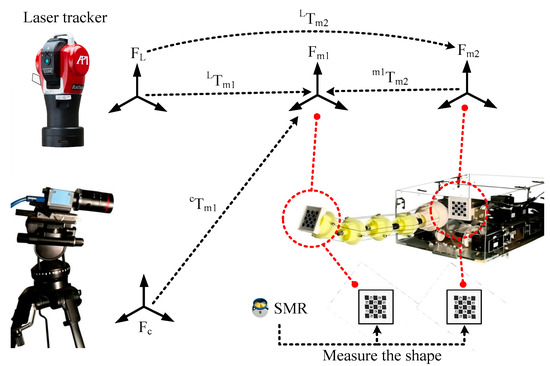
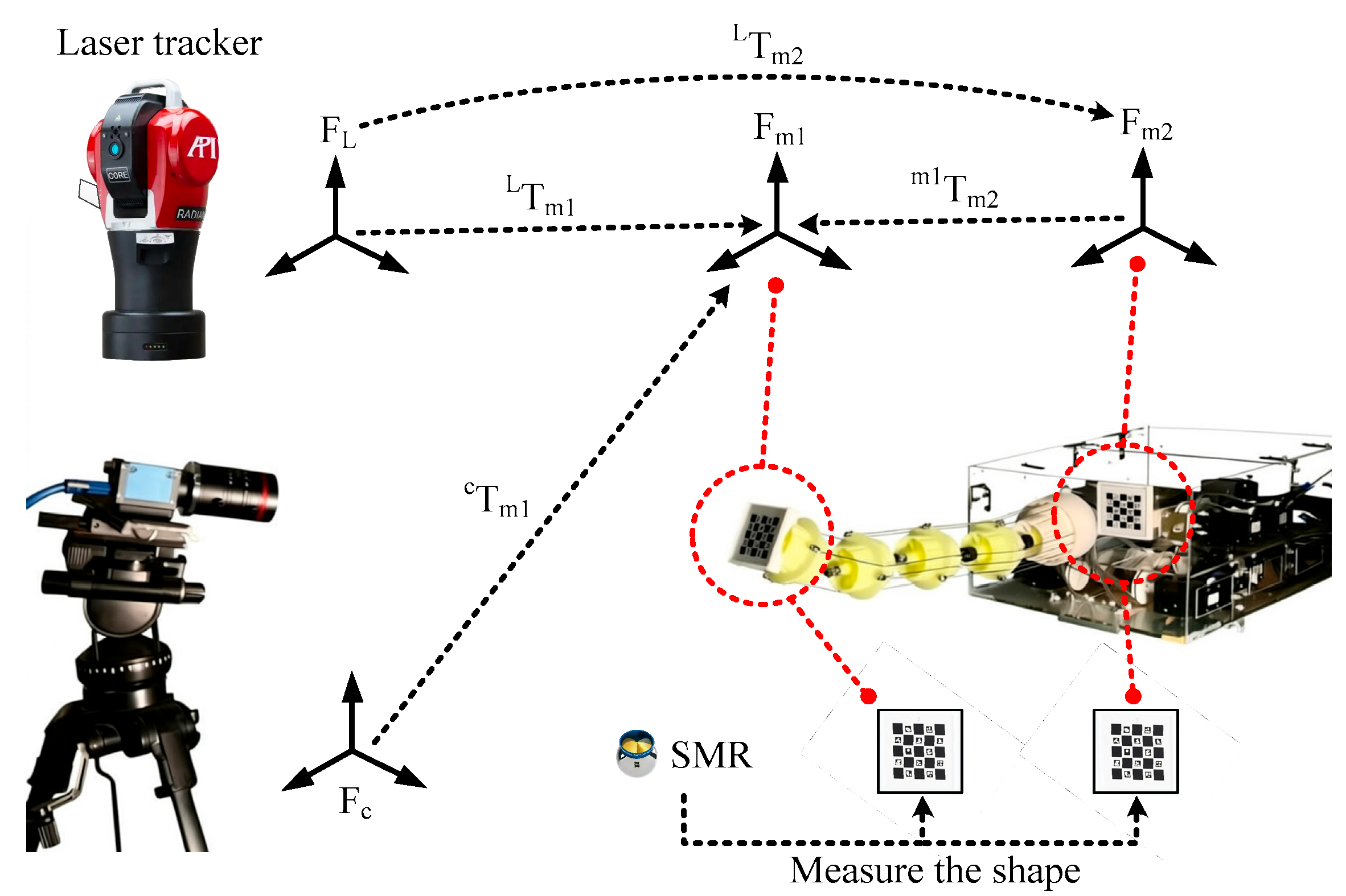
An API Radian PLUS laser tracker (API Metrology, Rockville, MD, USA) assists with registration of the measurement frames. Its specified distance resolution is 0.5 μm, and its maximum permissible error is 15 μm + 5 μm/m. The tracker provides a common reference for the markers, while the camera measures the lightweight end marker during calibration. The frame registration procedure is illustrated in Figure 12. Points on the edges and surface of marker-1 are measured with the tracker’s spherically mounted reflector (SMR), allowing the marker frame to be reconstructed in the tracker frame. Repeating this operation at different angles of joint 8 gives a sequence of marker poses. A circular fit to the marker origins determines the corresponding rotation axis. The axis of joint 7 is obtained in the same way. These axes, together with the adopted kinematic frame convention, establish the terminal frame and the constant transformation . To register the camera with the robot base, the tracker measures both marker frames, and the camera observes marker-1 at the same stationary configuration. With the fixed base-to-marker relationship , the transformations are chained as follows: = ()−1 .
Figure 12.
Establishment of 8Tm1 and cT0 with hybrid measurement instruments.
After the robot reaches each specified configuration, a settling time of approximately 5 s is allowed, and pose measurements are acquired once visible vibration has subsided. During SMR contact, the camera monitors marker-1 in real time to check for displacement caused by the probing force. At a measurement distance of 400 mm, the camera’s repeatability measurement accuracy is 0.06 mm along both the Xc and Yc axes and 0.13 mm along the Zc axis. Any contact-induced marker displacement should remain below the corresponding repeatability limits. The use of a lightweight visual marker limits the additional load at the tip of the compliant robot; the tracker is used for frame registration rather than carried by the robot during routine pose acquisition.
5.2. Pose Measurement and Parameter Identification
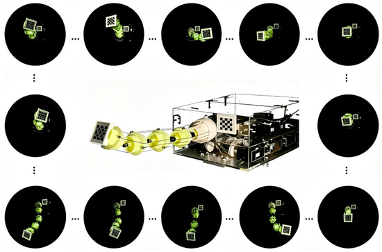
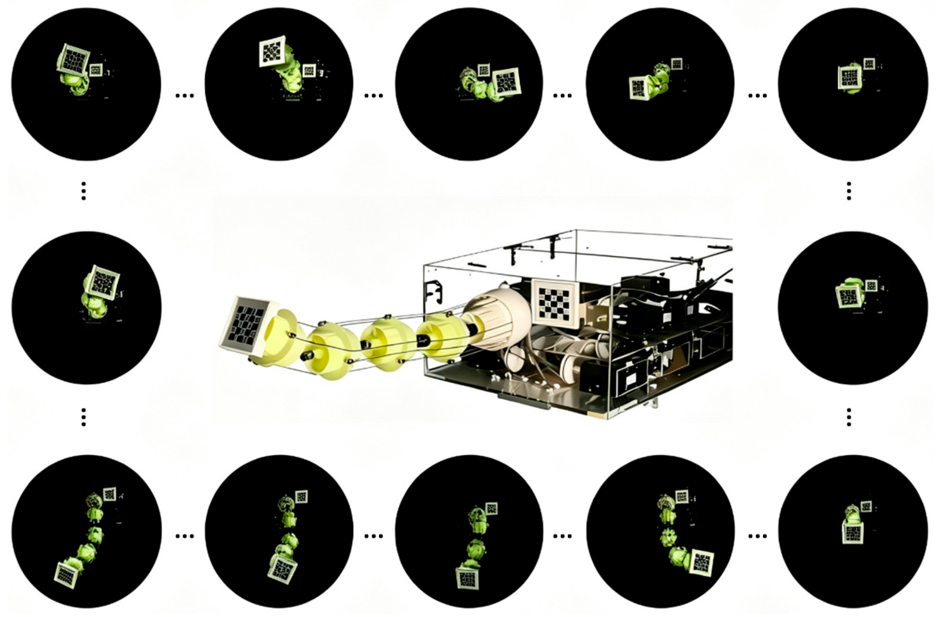
A total of 45 measurement configurations are selected using the DETMAX algorithm while accounting for marker visibility. The selected configurations vary the robot posture while maintaining a clear view of marker-1; representative configurations are shown in Figure 13. Configurations with severe occlusion or poor marker-image quality are excluded from pose acquisition. Each measurement configuration is performed five times and 30 images are captured for each marker after the robot has settled to reduce the influence of image noise on pose estimation at each measurement configuration.
Figure 13.
Some of the visible optimized measurement configurations.
The measured marker pose is converted into the pose of the terminal frame in the robot base frame using the registered transformations: = ()−1 ()−1. The discrepancy between the measured pose and the pose predicted by the calibration model supplies the observation data for parameter identification. The proposed identification method is denoted by M1, and the two comparison methods are denoted by M2 [20] and M3 [24], consistent with the labels in the experimental plots. Their iterative behavior is assessed through the norm of the parameter update, , whereas their practical calibration performance is assessed separately through the end-effector positioning residuals.
An additional set of 80 validation configurations is randomly generated to verify the calibration accuracy. The industrial camera is used to measure the end-effector positioning residuals at these validation configurations.
5.3. Experimental Results and Discussion
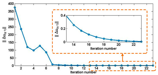
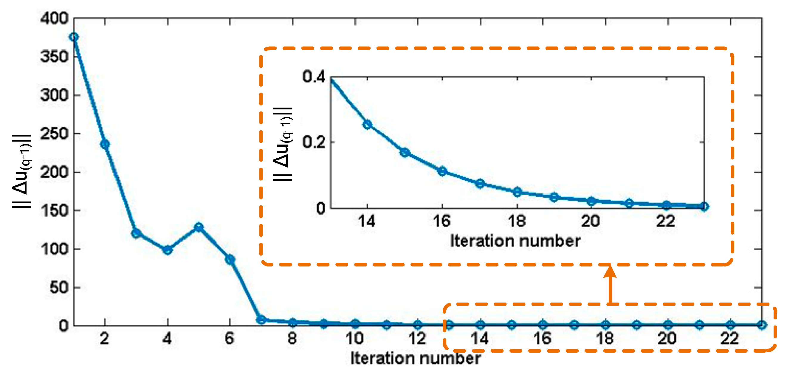
Figure 14, Figure 15 and Figure 16 show the evolution of for M1, M2, and M3 of the 1st repeated experiment, while the remaining results are given in Appendix B. All three curves exhibit an overall decrease followed by a small-update regime. For M1, the update norm falls from approximately 375 to below 10 within about seven iterations, despite a temporary increase near the fifth iteration. The inset in Figure 14 shows a smooth decrease from approximately 0.4 at iteration 13 to a value close to zero at the last plotted iteration, 23. The early increase is therefore transient and is not followed by sustained oscillation.
Figure 14.
Trend in ||Δu(q−1)|| with iteration number of M1 in experiment.
Figure 15.
Trend in ||Δu(q−1)|| with iteration number of M2 in experiment.
Figure 16.
Trend in ||Δu(q−1)|| with iteration number of M3 in experiment.
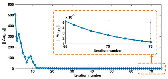
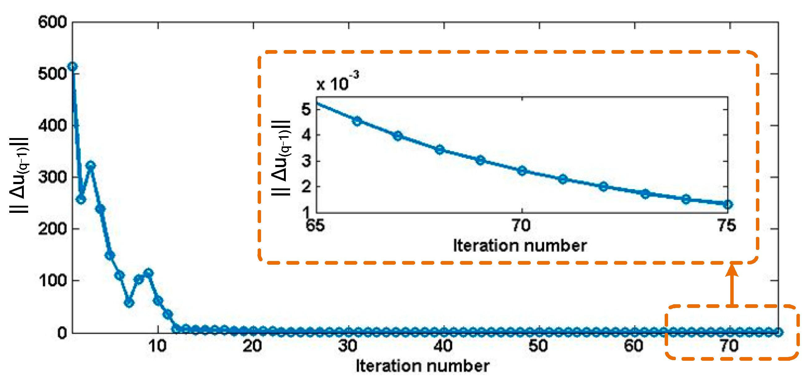
M2 also approaches a small update norm, as shown in Figure 15. Its initial decrease contains several reversals, particularly near iterations 3 and 8~9, before the curve enters a prolonged decay stage. The enlarged segment decreases from approximately 5 × 10⁻³ at iteration 65 to approximately 1.3 × 10⁻³ at iteration 75. Thus, the plotted result indicates continued stabilization, rather than divergence, although the recorded sequence is substantially longer than that of M1.
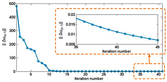
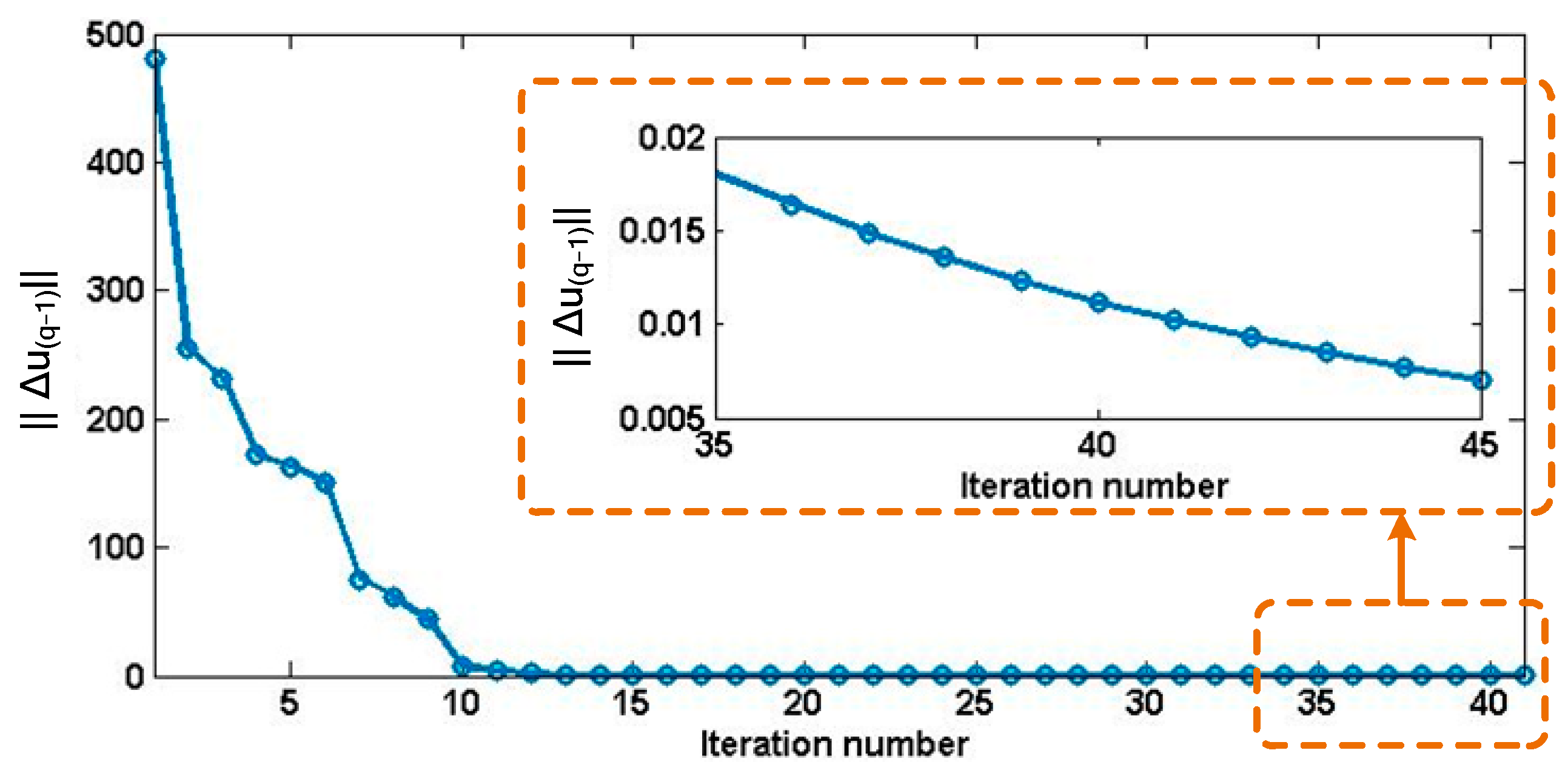
For M3, Figure 15 shows a rapid initial decrease from approximately 485, converging toward zero after iteration 10. The inset resolves its subsequent gradual decrease from approximately 0.018 at iteration 35 to approximately 0.007 at iteration 45. M3 therefore displays a shorter recorded iteration sequence than M2 and a longer sequence than M1.
The three recorded sequences end at iterations 23, 75, and 41, respectively. M1 thus uses the fewest iterations in the plotted runs and exhibits rapid stabilization after its initial transient. The time consumption of M1, M2 and M3 is 164.923 s, 473.494 s and 230.912 s, respectively, which is consistent with the difference in iteration numbers. M1 exhibits the fastest convergence speed. This may stem from the fact that M1 performs adaptive corrections directly on the identified results rather than indirectly adjusting the Jacobian matrix of the calibration model.
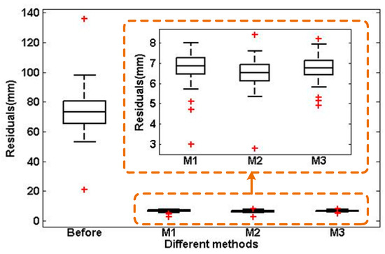
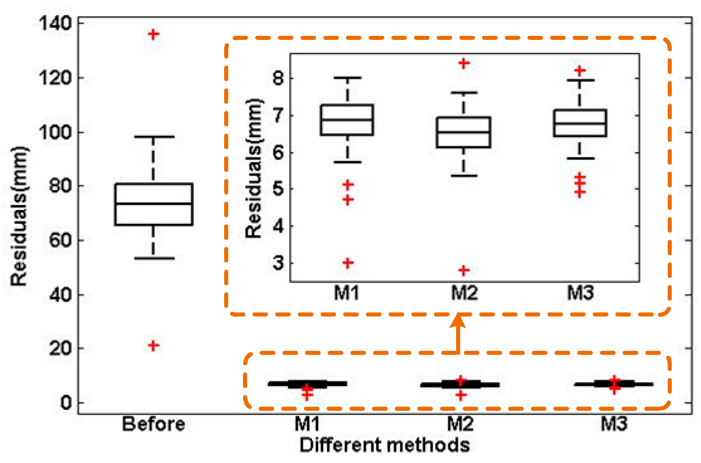
The positioning comparison in Figure 17 evaluates the uncalibrated robot and the robot after calibration with each of M1, M2, and M3. As the multiple identification results for M1, M2, and M3 in Appendix B show favorable repeatability, only the manipulator end-effector positioning residuals from the first experiment are shown herein. Specifically, the identified parameters are used to compute the compensated joint commands. For this cable-driven platform, those commands must then be converted into the corresponding cable-length changes and motor commands. The industrial camera measures the resulting end-effector positions after the robot settles. The absolute positioning residual is the Euclidean distance between the measured and desired end-effector positions, expressed in millimeters. The four groups in the figure represent the uncalibrated condition and three calibration methods.
Figure 17.
Comparison of absolute positioning residuals for different stages of new method in the 1st repeated experiment.
Figure 17 shows a marked reduction in positioning residuals for all three methods. Before calibration, the median is approximately 73 mm, with the central half of the observations spanning roughly 66~81 mm. The calibrated medians read from the inset are approximately 6.903 mm for M1, 6.612 mm for M2, and 6.756 mm for M3. These values correspond to a reduction of about 90% relative to the uncalibrated median. The three calibrated distributions nevertheless differ. M2 has the lowest median, while M1 and M3 have slightly higher medians than M2. However, the numerical differences among the residuals obtained by the three calibration methods are very small compared with those before calibration. Such minor differences cannot indicate the accuracy discrepancy of the three iterative algorithms, which implies that the three methods achieve identical iterative accuracy. This indicates that the proposed algorithm can maintain high iterative efficiency while attaining good convergence accuracy.
It should be noted that the analytical solution of Equation (16) attributes the gravity-induced joint deflection solely to the gravity moment MGi acting on the joint compliance λi. Friction in the joint hinges is not included in the compliance model, therefore constituting a major source of the discrepancy between the analytical solution and the experimental results. Another potential error source lies in the determination of the center of mass, i.e., the parameters Pgs and Pgl in Equations (4) and (5). However, since the resulting error in MGi is weighted by the relatively small lever arm of the combined center of mass and is further attenuated by the small joint compliance, its influence on the identified and compensated results is negligible compared with that of friction.
Millimeter-scale residuals remain after calibration. Plausible contributors include configuration-dependent cable friction, elastic deformation, transmission hysteresis, and uncertainty in visual measurement and frame registration. The results support a substantial improvement in positioning accuracy on the tested platform, while further characterization of mechanical and measurement effects is needed to explain and reduce the remaining errors.
6. Conclusions
This paper presents an elasto-geometrical calibration model and adaptive iterative identification algorithm for compliant hyper-redundant serial robots, enabling joint identification of kinematic geometric errors and joint elastic deformations. The adaptive weighting strategy effectively mitigates divergence triggered by high-dimensional parameters and linearization errors. Both simulation and experimental tests verify that the method delivers favorable calibration performance and faster convergence compared with existing approaches.
Several limitations still remain. First, the nonzero residuals and the variation across configurations indicate that further improvement in calibration accuracy is needed. Future work should characterize cable friction, hysteresis, and elastic deformation under controlled conditions and use the results to refine the model. Second, marker visibility limits the range of configurations accessible to a fixed camera. Viewpoint adjustment or multiple camera views, combined with configuration selection that considers parameter observability, could improve measurement coverage.
Author Contributions
Conceptualization, B.W.; methodology, B.W. and Z.J.; software, B.W. and Z.J.; validation, B.W.; formal analysis, B.W. and Z.J.; investigation, B.W. and Z.J.; resources, B.W.; data curation, B.W.; writing—original draft preparation, B.W. and S.X.; writing—review and editing, B.W. and S.X.; visualization, Z.J.; supervision, Z.J.; project administration, Z.J.; funding acquisition, Z.J. All authors have read and agreed to the published version of the manuscript.
Funding
This research was funded by the General Program of National Natural Science Foundation of China, grant number 52175452.
Institutional Review Board Statement
Not applicable.
Informed Consent Statement
Not applicable.
Data Availability Statement
Data is contained within this article.
Acknowledgments
During the preparation of this manuscript, the authors used Grammarly, v.1.2.304.1976 to improve the English language, grammar, and readability of the text. The authors reviewed and edited all AI-assisted content and take full responsibility for the final manuscript. The authors would also like to thank Beijing Beishute Maternity & Child Articles Co., Ltd for providing factory survey opportunities and technical support.
Conflicts of Interest
Author Bin Wang was employed by the company Beijing Beishute Maternity & Child Articles Co., Ltd. The remaining authors declare that the research was conducted in the absence of any commercial or financial relationships that could be construed as a potential conflict of interest.
Appendix A
If it is assumed that
Then, the analytical solution of VG is given by
Its three components are given by
The analytical solution of FGi is given by
Its three components are given by
Appendix B
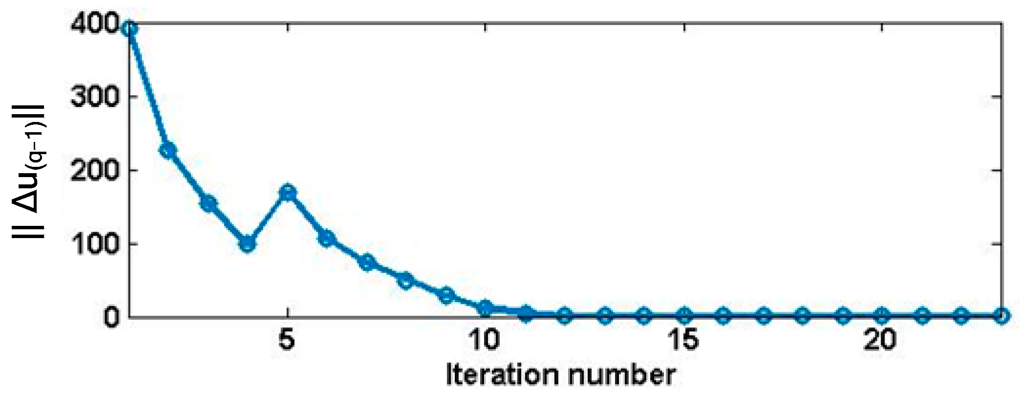
Results of the 2nd to 5th repeated experiments for Method M1 are given in Figure A1, Figure A2, Figure A3 and Figure A4.
Figure A1.
Trend in ||Δu(q−1)|| with iteration number of M1 in 2nd repeated experiment.
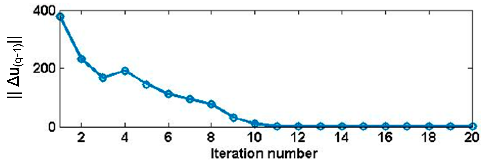
Figure A2.
Trend in ||Δu(q−1)|| with iteration number of M1 in 3rd repeated experiment.
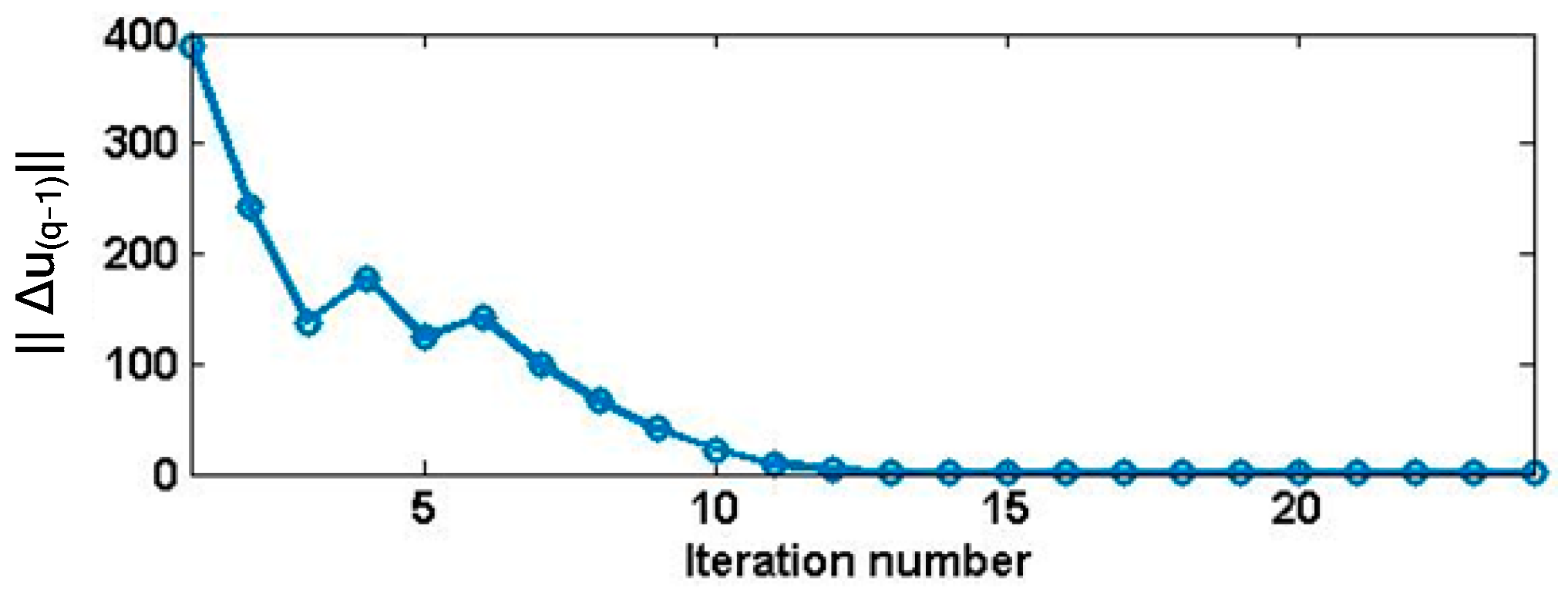
Figure A3.
Trend in ||Δu(q−1)|| with iteration number of M1 in 4th repeated experiment.
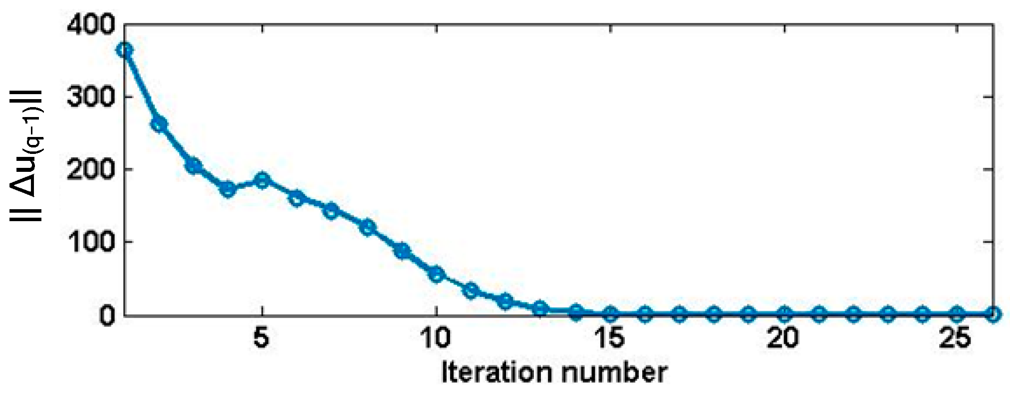
Figure A4.
Trend in ||Δu(q−1)|| with iteration number of M1 in 5th repeated experiment.
Results of the 2nd to 5th repeated experiments for Method M2 are given in Figure A5, Figure A6, Figure A7 and Figure A8.
Figure A5.
Trend in ||Δu(q−1)|| with iteration number of M2 in 2nd repeated experiment.
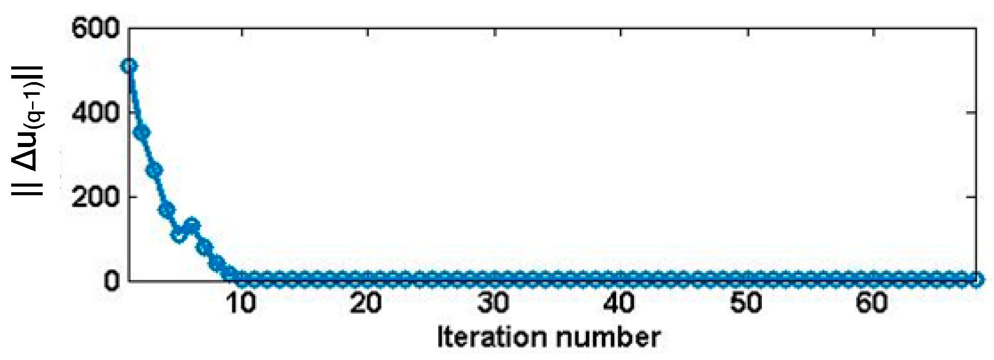
Figure A6.
Trend in ||Δu(q−1)|| with iteration number of M2 in 3rd repeated experiment.
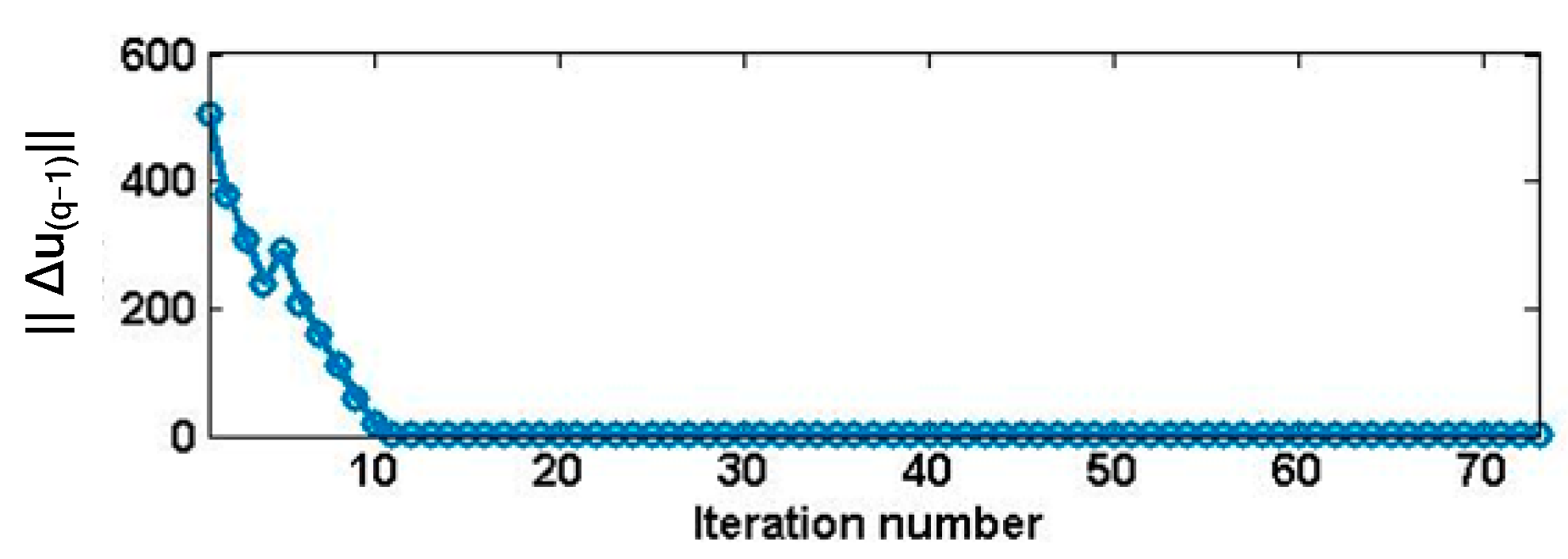
Figure A7.
Trend in ||Δu(q−1)|| with iteration number of M2 in 4th repeated experiment.
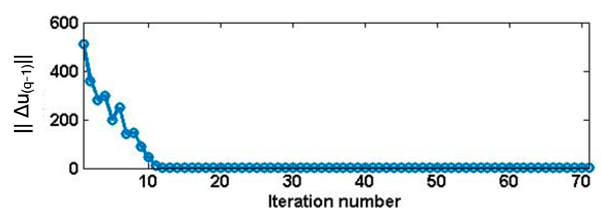
Figure A8.
Trend in ||Δu(q−1)|| with iteration number of M2 in 5th repeated experiment.
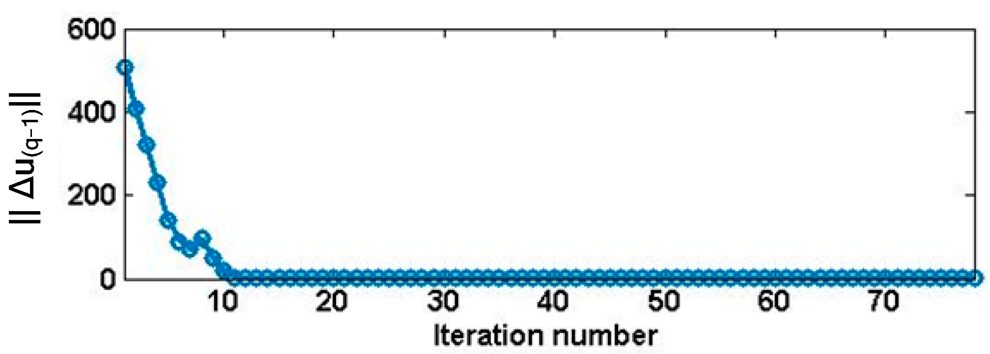
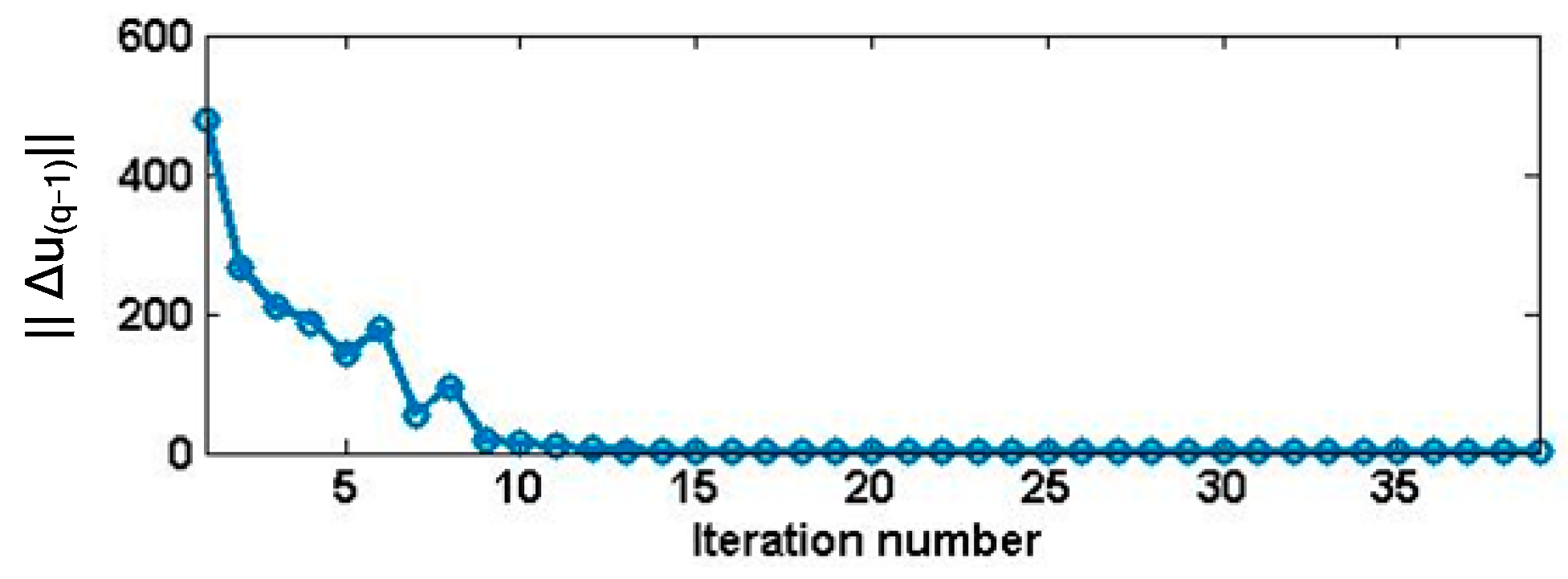
Results of the 2nd to 5th repeated experiments for Method M3 are given in Figure A9, Figure A10, Figure A11 and Figure A12.
Figure A9.
Trend in ||Δu(q−1)|| with iteration number of M3 in 2nd repeated experiment.
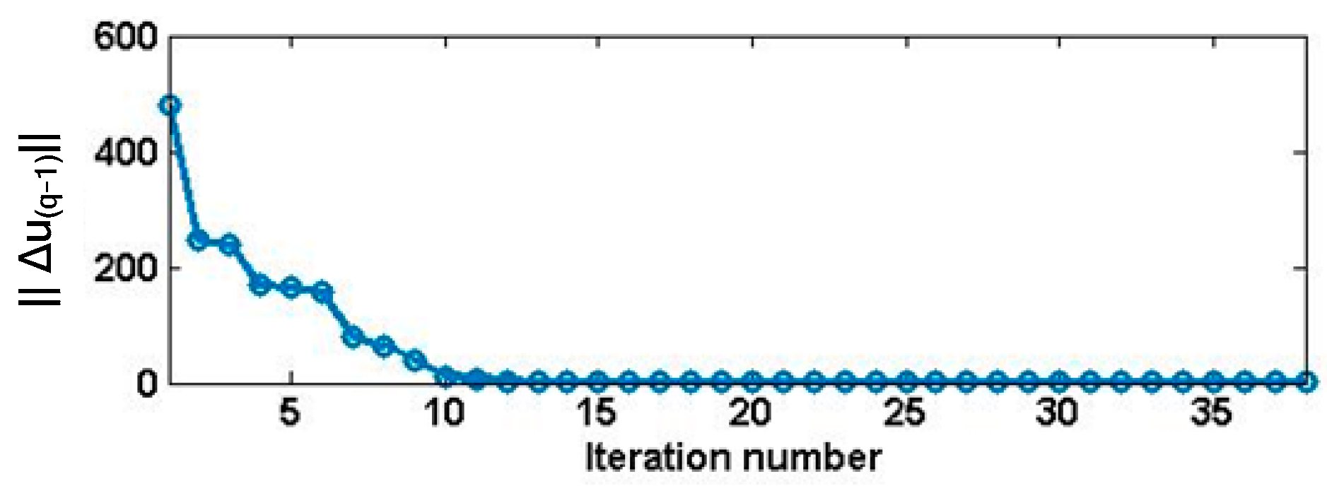
Figure A10.
Trend in ||Δu(q−1)|| with iteration number of M3 in 3rd repeated experiment.
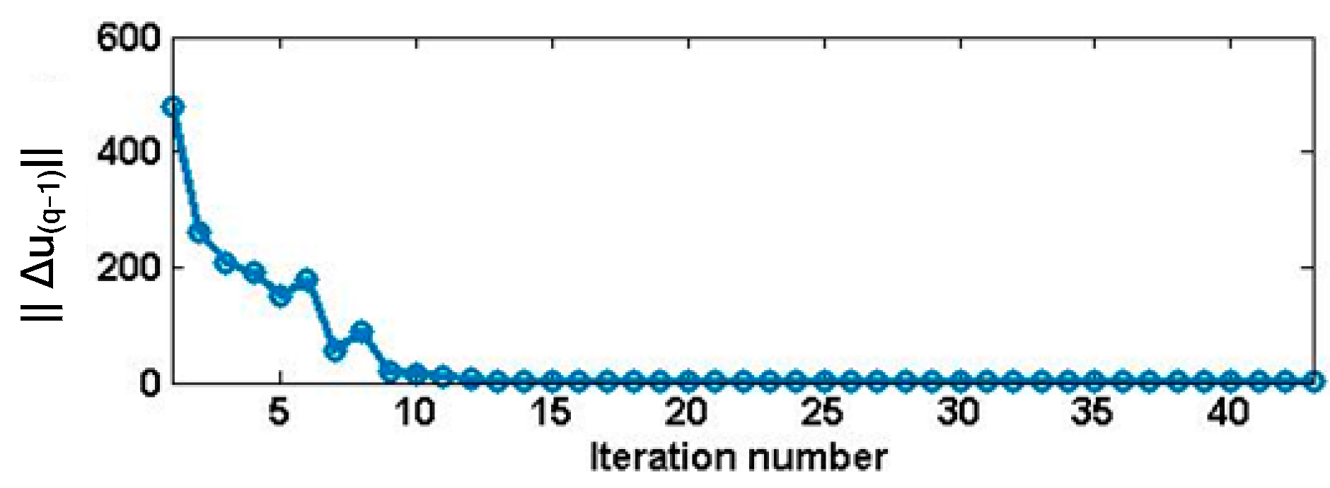
Figure A11.
Trend in ||Δu(q−1)|| with iteration number of M3 in 4th repeated experiment.
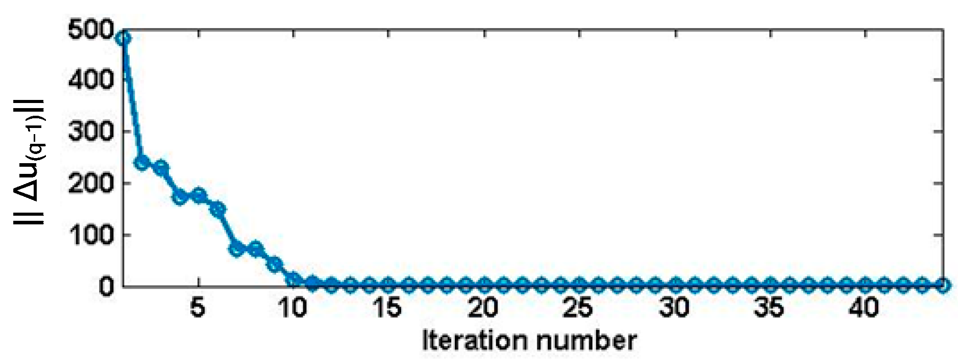
Figure A12.
Trend in ||Δu(q−1)|| with iteration number of M3 in 5th repeated experiment.
References
- Baizid, K.; Cukovic, S.; Iqbal, J.; Yousnadj, A.; Chellali, R.; Meddahi, A.; Devedžić, G.; Ghionea, I. IRoSim: Industrial robotics simulation design planning and optimization platform based on cad and knowledgeware technologies. Robot. Comput. Integr. Manuf. 2016, 42, 121–134. [Google Scholar] [CrossRef] [Scilit]
- Gang, C.; Tong, L.; Ming, C.; Xuan, J.Q.; Xu, S.H. Review on Kinematics Calibration Technology of Serial Robots. Int. J. Precis. Eng. Manuf. 2014, 15, 1759–1774. [Google Scholar] [CrossRef] [Scilit]
- Xu, W.; Liu, T.; Li, Y. Kinematics, Dynamics, and Control of a Cable-Driven Hyper-Redundant Manipulator. IEEE/ASME Trans. Mechatron. 2018, 23, 1693–1704. [Google Scholar] [CrossRef] [Scilit]
- Luo, M.; Li, E. A Bioinspired Coiled Cable-Driven Manipulator: Mechatronic Design and Kinematics Planning with Multiconstraints. IEEE/ASME Trans. Mechatron. 2023, 28, 3155–3166. [Google Scholar] [CrossRef] [Scilit]
- Bogue, R. Robots in the Nuclear Industry: A Review of Technologies and Applications. Ind. Robot Int. J. 2011, 38, 113–118. [Google Scholar] [CrossRef] [Scilit]
- Li, C.; Wu, Y.Q.; Lowe, H. POE-Based Robot Kinematic Calibration Using Axis Configuration Space and the Adjoint Error Model. IEEE Trans. Robot. 2016, 32, 1264–1279. [Google Scholar] [CrossRef] [Scilit]
- Chen, G.L.; Wang, H.; Lin, Z.Q. Determination of the Identifiable Parameters in Robot Calibration Based on the POE Formula. IEEE Trans. Robot. 2014, 30, 1066–1077. [Google Scholar] [CrossRef] [Scilit]
- Yang, X.D.; Wu, L.; Li, J.Q.; Chen, K. A Minimal Kinematic Model for Serial Robot Calibration Using POE Formula. Robot. Comput. Integr. Manuf. 2014, 30, 326–334. [Google Scholar] [CrossRef] [Scilit]
- Jiang, Z.; Su, R.; Liu, Y.; Long, Z.; Song, B.; Tang, X. Accurate Relative Measurement of Multi-Target Poses by Monocular Vision for Nonmodel-Based Real-Time Calibration of Industrial Robot. Measurement 2024, 235, 114979. [Google Scholar] [CrossRef] [Scilit]
- Jiang, Z.; Chen, S.; Zhao, Y.; Long, Z.; Song, B.; Tang, X. Accurate Kinematic Calibration of a Six-DoF Serial Robot by Using Hybrid Models with Reduced Dimension and Minimized Linearization Errors. Ind. Robot Int. J. Robot. Res. Appl. 2024, 51, 772–788. [Google Scholar] [CrossRef] [Scilit]
- Jiang, Z.; Ding, R.; Liu, Y.; Long, Z.; Song, B. Vision-Based and Real-Time Calibration of Industrial Robot by Using Deep Learning and Dimension-Reduced Models. Precis. Eng. 2025, 96, 192–211. [Google Scholar] [CrossRef] [Scilit]
- Nubiola, A.; Slamani, M.; Bonev, I.A. A New Method for Measuring a Large Set of Poses with a Single Telescoping Ballbar. Precis. Eng. 2013, 37, 451–460. [Google Scholar] [CrossRef] [Scilit]
- Nubiola, A.; Bonev, I.A. Absolute Robot Calibration with a Single Telescoping Ballbar. Precis. Eng. 2014, 38, 472–480. [Google Scholar] [CrossRef] [Scilit]
- Nubiola, A.; Bonev, I.A. Non-Kinematic Calibration of a Six-Axis Serial Robot Using Planar Constraints. Precis. Eng. 2015, 40, 472–480. [Google Scholar] [CrossRef] [Scilit]
- Nubiola, A.; Bonev, I.A. Absolute Calibration of an ABB IRB 1600 Robot Using a Laser Tracker. Robot. Comput. Integr. Manuf. 2013, 29, 236–245. [Google Scholar] [CrossRef] [Scilit]
- Klimchik, A.; Furet, B.; Caro, S.; Pashkevich, A. Identification of the Manipulator Stiffness Model Parameters in Industrial Environment. Mech. Mach. Theory 2015, 90, 1–22. [Google Scholar] [CrossRef] [Scilit]
- Gong, C.H.; Yuan, J.X.; Ni, J. Nongeometric Error Identification and Compensation for Robotic System by Inverse Calibration. Int. J. Mach. Tools Manuf. 2000, 40, 2119–2137. [Google Scholar] [CrossRef] [Scilit]
- Chen, S.F.; Kao, I. Conservative Congruence Transformation for Joint and Cartesian Stiffness Matrices of Robotic Hands and Fingers. Int. J. Robot. Res. 2000, 19, 835–847. [Google Scholar] [CrossRef] [Scilit]
- Dumas, C.; Caro, S.; Garnier, S.; Furet, B. Joint Stiffness Identification of Six-Revolute Industrial Serial Robots. Robot. Comput. Integr. Manuf. 2011, 27, 881–888. [Google Scholar] [CrossRef] [Scilit]
- Zhou, J.; Nguyen, H.N.; Kang, H.J. Simultaneous Identification of Joint Compliance and Kinematic Parameters of Industrial Robots. Int. J. Precis. Eng. Manuf. 2014, 15, 2257–2264. [Google Scholar] [CrossRef] [Scilit]
- Mamedov, S.; Popov, D.; Mikhel, S.; Klimchik, A. Compliance Error Compensation Based on Reduced Model for Industrial Robots. In Proceedings of the International Conference on Informatics in Control, Automation and Robotics (ICINCO), Porto, Portugal, 29–31 July 2018. [Google Scholar]
- Theissen, N.A.; Laspas, T.; Archenti, A. Closed-Force-Loop Elastostatic Calibration of Serial Articulated Robots. Robot. Comput. Integr. Manuf. 2019, 57, 86–91. [Google Scholar] [CrossRef] [Scilit]
- Du, L.; Zhang, T.; Dai, X.L. Compliance Error Calibration for Robot Based on Statistical Properties of Single Joint. J. Mech. Sci. Technol. 2019, 33, 1861–1868. [Google Scholar] [CrossRef] [Scilit]
- Chen, X.Y.; Zhang, Q.J.; Sun, Y.L. Non-Kinematic Calibration of Industrial Robots Using a Rigid-Flexible Coupling Error Model and a Full Pose Measurement Method. Robot. Comput. Integr. Manuf. 2019, 57, 46–58. [Google Scholar] [CrossRef] [Scilit]
- Sun, T.; Liu, C.; Lian, B.; Wang, P.; Song, Y. Calibration for Precision Kinematic Control of an Articulated Serial Robot. IEEE Trans. Ind. Electron. 2021, 68, 6000–6009. [Google Scholar] [CrossRef] [Scilit]
- Luo, G.; Zou, L.; Wang, Z.; Lv, C.; Ou, J.; Huang, Y. A novel kinematic parameters calibration method for industrial robot based on Levenberg-Marquardt and Differential Evolution hybrid algorithm. Robot. Comput. Integr. Manuf. 2021, 71, 102165. [Google Scholar] [CrossRef] [Scilit]

Disclaimer/Publisher’s Note: The statements, opinions and data contained in all publications are solely those of the individual author(s) and contributor(s) and not of MDPI and/or the editor(s). MDPI and/or the editor(s) disclaim responsibility for any injury to people or property resulting from any ideas, methods, instructions or products referred to in the content. |
© 2026 by the authors. Licensee MDPI, Basel, Switzerland. This article is an open access article distributed under the terms and conditions of the Creative Commons Attribution (CC BY) license.