


Abstract
To complete scientific experiments on an underwater tension leg platform, a new cable-driven underwater vehicle is proposed, which is subjected to not only unknown underwater disturbances but also time-varying nonlinear cable tractions. To achieve displacement tracking control despite the high-order nonlinearities and matched and mismatched uncertainties with unknown upper bounds, a radial basis function neural network-based adaptive multiple-surface sliding control strategy (RBFNN-AMSC) is proposed. Utilizing a backstepping design procedure and the Lyapunov approach, the system is decomposed into six subsystems, and the stability is ensured. By employing multiple-surface sliding mode control and exponential reaching law design, the robustness and convergence rate of each subsystem are improved. Moreover, with an adaptive radial basis function neural network, the influences of matched and mismatched uncertainties are compensated, which improves the system anti-jamming capability and avoids the “differential explosion” problem. To verify the effectiveness of the proposed approach, numerical simulations are carried out under different conditions, which show that the proposed control strategy can achieve accurate displacement tracking control regardless of complex nonlinear dynamics and various unknown external disturbances.
1. Introduction
In recent years, underwater vehicles have played an increasingly important role in ocean exploration [1,2,3]. Conventional underwater vehicles, including ROVs and AUVs, are flexible in movement, but their carrying capacity is often limited due to the constrained space and power, making them unsuitable for heavy-load handling tasks. In order to conduct an underwater experiment involving heavy-load transportation, this paper proposes a novel cable-driven underwater vehicle inspired by cable-driven systems [4].
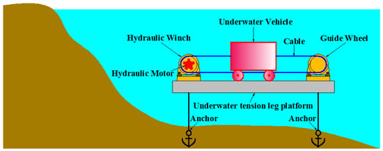
The system is installed on an underwater tension leg platform [5], and it mainly consists of a hydraulic winch, an underwater vehicle, a cable, and a guide wheel. Under the traction of the winch, the underwater vehicle performs linear reciprocating motion along a fixed guide rail on the platform. Compared to conventional towed underwater vehicles [6], the proposed structure significantly restricts the vehicle’s freedom of movement, enhances the stability of the system, and makes towing with large loads possible. Although the structure of this system appears simple and more stable than typical underwater robots, it not only has to contend with cable fluctuation disturbances encountered in conventional underwater towed vehicles [7] but also has to deal with load fluctuations and complex hydrodynamic effects. Moreover, owing to the special demands of scientific experiments, the underwater vehicle is required to accomplish accurate displacement control. Therefore, dynamic modeling and controller design are quite challenging.
In the past few decades, considerable efforts have been made in modeling cable-driven systems and underwater vehicles [8]. Li et al. modeled a dual-cable tendon–sheath transmission as a bidirectionally coupled dynamic subsystem and developed a distributed spring friction-unit formulation that explicitly links routing geometry, pretension, and distal dynamics to transmitted torque, hysteresis, and apparent stiffness variation [9]. A novel un-stretched length consistency constraint was introduced to replace rigid geometric assumptions, accurately capturing the differential sagging inherent in parallel cable mechanisms under eccentric loading [10]. An angle identification model was established by Tan et al. to achieve real-time detection and compensation of cable bending angles for cable-driven actuation systems [11]. A new analytical model was established for the drum–rope interaction in mechanical systems actuated through ropes or cables, which consisted of a set of analytical force–displacement relations that captured the extensibility of the rope and the drum–rope contact interaction, assuming linear elastic behavior and Coulomb friction [12]. To study the dynamic characteristics of a cyclic towing system, Lagrange equations and the Runge–Kutta method were utilized by Luo and He [13]. In [14], a novel method was designed to estimate the model for a towed underwater vehicle, based on which the depth and posture control algorithm was designed. The system studied in this paper combines the characteristics of both cable-driven systems and underwater vehicles. Considering the coupled dynamics of the vehicle and the cable, as well as various unknown underwater disturbances, the system reveals quite complex nonlinear dynamics [15]. In this paper, the cable tension is regarded as a third-order nonlinear function. By comprehensively considering the changes in cable tension, water resistance, and unknown environmental disturbances, a high-order nonlinear dynamic model is ultimately obtained.
Owing to complex nonlinearities and unknown disturbances, designing a controller to regulate the underwater cable-driven vehicle is not easy. For complex nonlinear systems with uncertainties, the commonly used control methods include, but are not limited to, H∞ control [16], adaptive control [17], sliding mode control [18], fuzzy logic control [19], backstepping control [20], and neural network methods [21].
The parameter uncertainties and unknown external disturbances should be taken into account since they could severely degrade the closed-loop system performance [22]. In the past few decades, neural networks and disturbance observers have been two of the main solutions for uncertainty estimation. A fixed-time sliding mode extended state observer was proposed by Huo et al. to estimate lumped disturbances for a cable-driven wave motion compensation device, which encompassed both unmodeled dynamics and external disturbances [23]. Ginoya et al. proposed an extended disturbance observer-based sliding mode control method for general nth order systems with mismatched uncertainties [24]. Li et al. proposed an adaptive neural tracking control scheme for uncertain nonlinear systems with input and output constraints, which introduced a Nussbaum function to handle the input saturation, and employed a disturbance observer to estimate unknown external disturbances [25]. A predefined-time trajectory tracking controller was designed by Zou et al. using radial basis function neural networks for the trajectory tracking control of a rigid–flexible cable-driven space manipulator [26].
Meanwhile, since the model estimation accuracy cannot be absolutely guaranteed, the robustness of the control scheme is of major importance. Sliding mode control is one of the most widely used methods for nonlinear systems since it can enhance the robustness of a control system regardless of external disturbances and parameter variations. However, due to the chattering problem, scholars have been integrating other methods with sliding mode control in recent years. An adaptive integral terminal sliding mode control method with a nonlinear extended state observer (NESO-AITSMC) was proposed by Zhang et al. to achieve disturbance rejection control for nonlinear cable-driven continuum robots under multi-source disturbance coupling [27]. Ding et al. proposed a novel composite control strategy for a cable-driven aerial manipulator, integrating proxy-based sliding mode control and a linear extended state observer technique [28]. A supervisory interval type-2 fuzzy adaptive sliding mode control scheme was proposed by Aghaseyedabdollah et al. for cable robots, which combined intelligent methods with conventional sliding mode control to achieve optimal adjustment of control parameters, thus ensuring accurate tracking performance, despite the structural constraints of cable robots [29].
Motivated by prior works and the above considerations, a novel RBFNN-AMSC method is proposed for the underwater cable-driven vehicle subject to unknown disturbances. The main contributions can be summarized as follows.
(1) A backstepping multiple-surface sliding control framework is proposed, which decomposes the complex high-order nonlinear system into six subsystems and establishes multiple sliding mode surfaces for the whole system. Compared with the conventional sliding mode control method, the proposed control framework is simplified. Meanwhile, through multiple sliding surfaces and exponential reaching law design, the robustness and convergence rate of each subsystem are improved.
(2) Considering the fact that system uncertainties do not satisfy the matching condition and the upper bounds of the uncertainties are not available, as well as to avoid the “differential explosion” problem, adaptive RBFNN is utilized to achieve compound disturbance estimation. Therefore, the influences of compound uncertainties with unknown upper bounds can be compensated, thus improving the anti-jamming capability.
The rest of this work is organized as follows. Section 2 establishes the dynamic model and formulates the displacement tracking control problem. Section 3 proposes the RBFNN-AMSC strategy and presents the detailed deriving and proving process. Section 4 validates the previous analysis and design through three simulation cases and discussions. Section 5 demonstrates the conclusions of this work.
2. Modeling and Problem Formulation
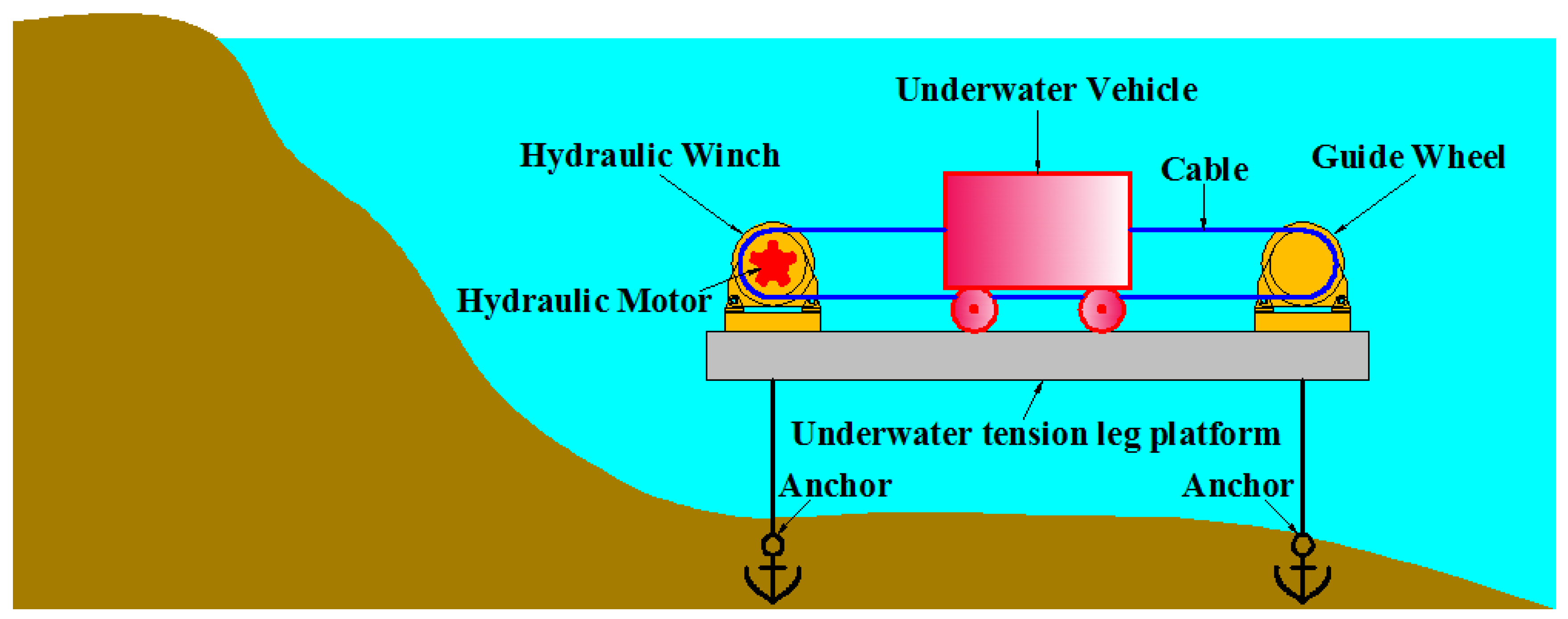
As shown in Figure 1, the cable-driven underwater vehicle system is installed on an underwater tension leg platform. Driven by the hydraulic winch and closed-loop cable-wheel system, the underwater vehicle is regulated to move along a guide rail on the platform. During its movement, the underwater vehicle is subjected not only to the tension from the two cables at the front and rear, but also to the resistance of water and the friction between it and the guide rail.
Figure 1.
Application description of underwater cable-driven vehicle system.
Theoretically, when the system operates stably, the deformation of the front and rear cables remains relatively constant, and the velocities of the winch, underwater vehicle, and guide wheel are essentially identical. However, in practice, due to the continuous changes in the velocity of the underwater vehicle and the resulting variations in water resistance, there will be deviations in the velocities of the winch, underwater vehicle, and guide wheel. This, in turn, leads to different amounts of stretching and contraction in the front and rear cables, causing internal tension changes in the cables. Therefore, during the modeling process, it is necessary to fully consider the tension changes caused by cable deformation.
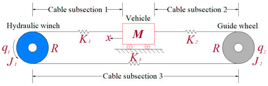
To facilitate dynamic modeling, a simplified schematic model is proposed in Figure 2, and the following assumptions are required.
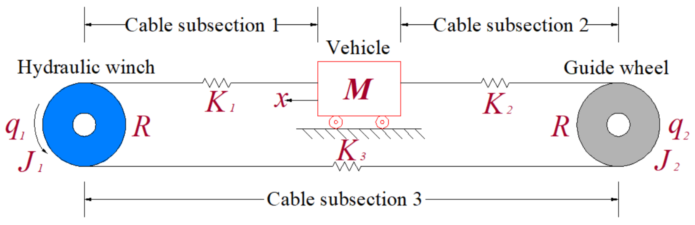
Figure 2.
Schematic model of underwater cable-driven vehicle system.
Assumption 1.
The underwater vehicle, hydraulic winch, and guide wheel are all rigid bodies.
Assumption 2.
With the support of the tension legs, the position of the underwater tension leg platform is very stable; the pitch and roll angles can be considered as 0°, which will not affect the control of the cable-driven underwater vehicle.
To analyze the changes in cable tension more clearly, the cable is divided into three subsections, as shown in Figure 2. In each cable segment, the inconsistent speeds of the front and rear endpoints cause deformation of the cable, which in turn leads to tension fluctuations. Inspired by [30], the cable tensions in the system are described as , where denotes the deformation of the cable, and are stiffness coefficients. In this paper, the deformation of the cable is calculated by the difference in displacement between the two end points of each subsection of the cable.
According to Newton’s second law of motion and the law of fixed-axis rotation of a rigid body, the dynamic models of an underwater cable-driven system can be described as follows.
where represents the mass of the vehicle, is the added mass caused by the relative motion between the vehicle and water, is the displacement of the vehicle, denotes the radius of hydraulic winch and guide wheel, denote the angular displacements of hydraulic winch and guide wheel, denote the moments of inertia of hydraulic winch and guide wheel, denotes the friction between vehicle and pathway, denotes the water resistance, where is the drag force coefficient of the underwater vehicle, is the water density, is the sectional area of underwater vehicle in the direction of motion, denote other unknown external disturbances, caused by the unknown underwater disturbances, time-varying hydraulic parameters, and the leak of hydraulic systems, etc., denotes the reduction ratio, is the output torque of hydraulic winch.
The system states and control input are defined as follows.
Therefore, the dynamic model of underwater cable-driven vehicle system is rewritten as
where denote compound unknown uncertainties, denote known nonlinear functions, the specific expressions of which are shown below.
Our objective is to develop a tracking control algorithm to make the underwater vehicle reach the desired displacement according to the requirements, regardless of system nonlinearities and unknown disturbances.
The problem is mathematically stated as follows: Given the system dynamic model Equation (4) and desired vehicle displacement , derive an effective control law to generate the control input , so that the displacement error can converge to zero.
To facilitate controller design in the next section, the following assumptions are required.
Assumption 3.
There exist positive constants such that the desired trajectory and its time derivatives satisfy .
Assumption 4.
There exist positive unknown constants
such that the unknown disturbances satisfy .
3. Controller Design
3.1. Control Strategy Analysis
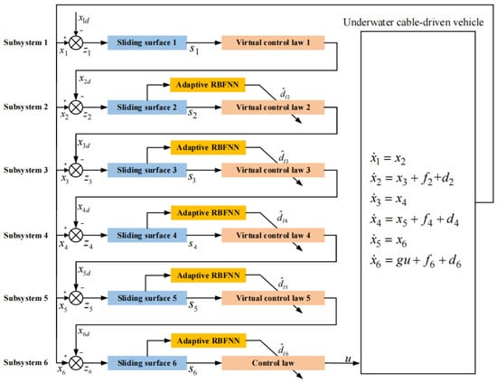
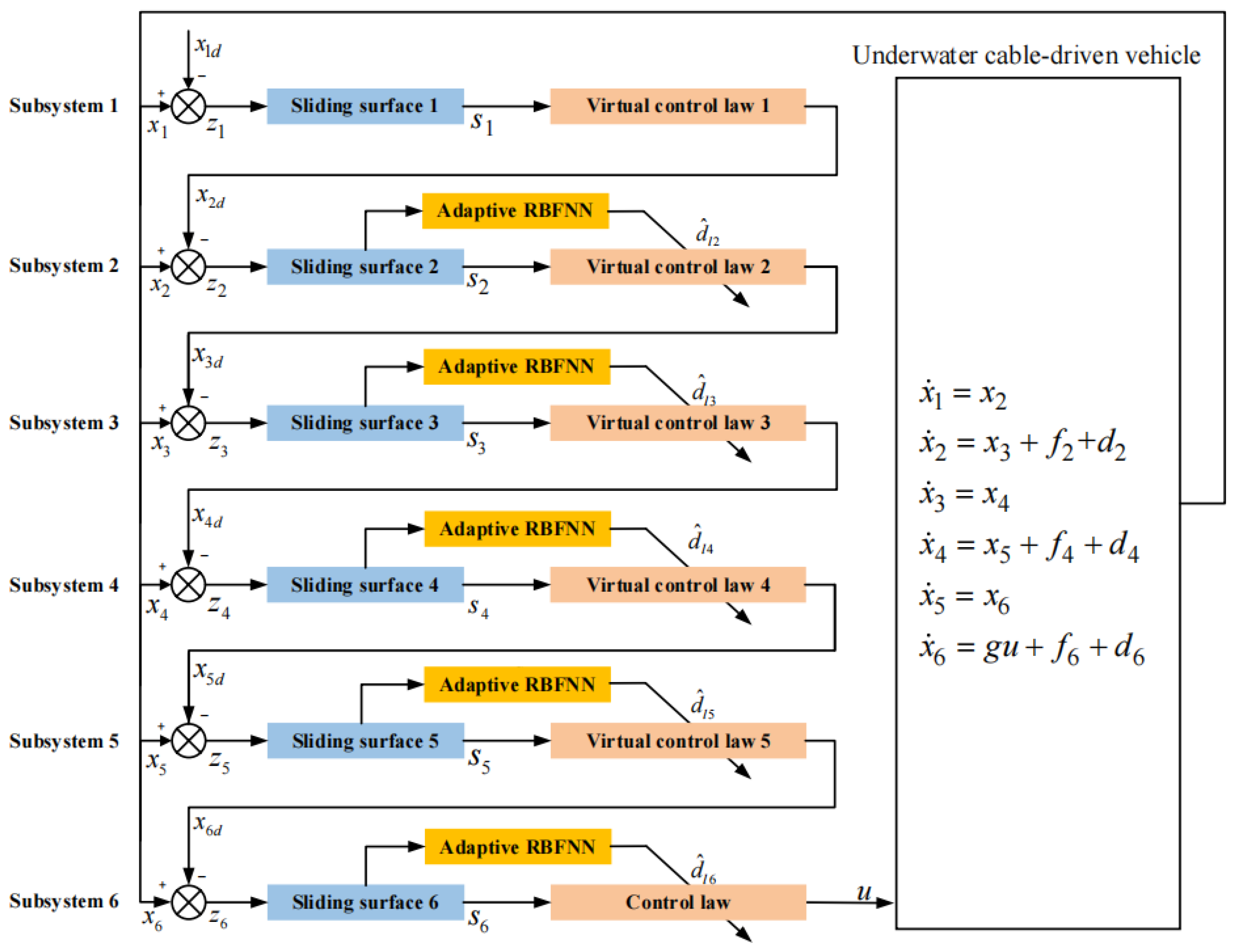
To achieve high-precision displacement tracking control regardless of the high-order nonlinearities, matched and mismatched uncertainties with unknown upper bounds, as well as external disturbances, a RBFNN based adaptive multiple-surface sliding control strategy is proposed, as shown in Figure 3.
Figure 3.
RBFNN-based adaptive multiple-surface sliding control strategy.
The main features and advantages of the proposed control strategy can be summarized as follows.
- (1)
- Adaptive backstepping design. The backstepping design procedure is chosen as the main framework of this control strategy, which decomposes the high-order nonlinear system into six subsystems. Lyapunov function and intermediate virtual control law are designed in each subsystem until the whole algorithm design is finished. Moreover, to avoid the “differential explosion” problem, the RBFNN is introduced to deal with the complex calculation part. Through the backstepping procedure and Lyapunov approach, the complex system is simplified, and the stability of the control algorithm is ensured.
- (2)
- Multiple-surface sliding control. Unlike the conventional backstepping sliding mode control method, a sliding surface is designed for each subsystem in the proposed approach, taking into account the issue of large initial deviation; thus, multiple sliding surfaces are established for the whole system. Through multiple sliding surfaces and exponential reaching law design, the robustness and convergence rate of each subsystem are improved.
- (3)
- Adaptive RBF neural network. Since the system contains various matched and mismatched disturbances with unknown upper bounds, an adaptive RBF neural network is utilized for disturbance estimation in intermediate virtual and actual control law design, it has been proved that the RBF neural network has the ability to approximate any continuous function with arbitrary precision. Hence, the influences of matched and mismatched disturbances with unknown upper bounds can be compensated, thus improving the system’s robustness.
3.2. RBFNN-AMSC Controller Design
Step 1: Define the error state variable and sliding surface for subsystem 1 as
where is the desired value of vehicle position, is the user-defined parameter, denotes the initial value of error state variable . Adopting such a method can make the initial magnitude of sliding variables always be zero, which helps resolve the problem of large initial conditions.
The time derivative of the first sliding surface is derived as
To help facilitate the fast approaching of the sliding mode surface, the following exponential reaching law is adopted:
Then, the virtual control input is designed as follows.
Theorem 1.
For the dynamic subsystem 1, if
converges to zero, the tracking error converges to zero with the virtual control law .
Proof.
Consider the following Lyapunov function candidate
The time derivative of Equation (11) is derived as
Apparently, if converges to zero, holds for all , which implies can converge to a small neighborhood of zero. □
Step 2: Define the error state variable and sliding surface of subsystem 2 as
where is the designed virtual control law in step 1, is the user-defined parameter, denotes the initial value of the error state variable .
Considering Equation (4) and differentiating with respect to time, one can obtain
According to Equation (10), is calculated as
It is obvious that the calculation of is complex and will bring considerable workloads. The situation will be more and more serious as the backstepping procedure goes on, which may eventually lead to the “differential explosion” problem. In order to simplify the calculation, Equation (16) is rewritten as
where is the complex part of , which is hard to calculate.
Considering Equations (15) and (17), the time derivative of can be calculated as
Define , Equation (18) is rewritten as
where denotes the compound disturbance, which contains model uncertainty and a complex calculation part.
To facilitate the controller design procedure, the following assumption is required.
Assumption 5.
There exist positive unknown constants
such that the compound disturbances satisfy .
Since is unknown, the following RBFNN function is used to estimate the compound disturbance.
where and denote the estimate weight matrix and center of the Gaussian basis function, respectively.
The Gaussian basis function is designed as follows.
where is the width of the Gaussian basis function.
Utilizing Equation (20), the compound disturbance is written as
where denotes the estimate error of .
Since an RBF neural network has the ability to approximate any continuous function with arbitrary precision, can be rewritten as
where and are the optimal weight and center of the Gaussian basis function, respectively, denotes the minimum approximation error.
Substituting Equation (23) into Equation (19) yields
In order to make subsystem 2 converge onto the sliding manifold with an exponential reaching law, the virtual control law of subsystem 2 is designed as
where , and the parameter updating laws are designed as:
where .
Theorem 2.
If
converges to zero, the dynamic subsystem 2 is stable under the proposed virtual control law .
Proof.
Consider the following Lyapunov function candidate:
where , , and denote the estimate errors, which are defined as , , and .
Considering Equation (24) and differentiating with respect to time, one can obtain
Substituting Equation (25) into Equation (28) yields
Since
where is the partial derivative of with respect to , and is the higher-order term. Let , and assume is bounded with , then Equation (29) can be rewritten as
Substituting Equation (26) into Equation (31) yields
where , .
If , Equation (32) can be further derived as
Obviously, it is always possible to select and to satisfy . Therefore, it can be concluded from Equation (33) that as long as . Consequently, the decrease of will drive into the boundary . Furthermore, according to Equation (14), the convergence of proves the convergence of .
Therefore, it is proved that under the influence of virtual control input , subsystem 2 is stable. This completes the proof. □
Step 3: Define the error state variable and sliding surface of subsystem 3 as
where is the user-defined parameter, denotes the initial value of error state variable .
To avoid the “differential explosion” problem and simplify the calculation, is rewritten as
where denotes the complex part of , which is hard to calculate.
Differentiating with respect to time, one can obtain
where denotes the compound disturbance, and .
In order to make subsystem 3 converge onto the sliding manifold with an exponential reaching law, the virtual control law of subsystem 3 is designed as
where .
The parameter updating law of RBFNN is designed as follows.
where .
Consider the following Lyapunov function candidate.
where , , and denote the estimate errors, which are defined as , , and . , , and are designed parameters.
Adopting a similar deriving method, one can obtain
As proved in Theorem 2, the following conclusion can be obtained: If converges to zero, the dynamic subsystem 3 discussed in step 3 is stable under the proposed virtual control law .
Step 4: Define the error state variable and sliding surface of subsystem 4 as
where is the user-defined parameter, denotes the initial value of error state variable .
Similar to step 2, the time derivative of can be described as follows:
where is the optimal RBFNN estimation of compound disturbance , and denotes the optimal estimate error.
The virtual control law is designed as
where .
The parameter updating law of RBFNN is designed as follows:
where .
Utilizing the same proving method, one can obtain: If converges to zero, the dynamic subsystem 4 discussed in step 4 is stable under the proposed virtual control law .
Step 5: Define the error state variable and sliding surface of subsystem 5 as
where is the user-defined parameter, denotes the initial value of error state variable .
Similar to step 3, the time derivative of can be obtained as follows:
where is the optimal RBFNN estimation of compound disturbance , and denotes the minimum estimate error.
In order to make subsystem 5 converge onto the sliding manifold with an exponential reaching law, the virtual control law is designed as
where .
The parameter updating law of RBFNN is designed as follows:
where .
Utilizing the same proving method, one can obtain: If converges to zero, the dynamic subsystem 5 discussed in step 5 is stable under the proposed virtual control law .
Step 6: Define the error state variable and sliding surface of subsystem 6 as
where is the user-defined parameter, denotes the initial value of error state variable .
Differentiating with respect to time, one can obtain
where denotes the compound disturbances, which contains model disturbance and the complex calculation part, and , denotes the complex calculation part of , and . and are optimal RBFNN estimation and optimal estimate error of , respectively.
In order to make subsystem 6 converge onto the sliding manifold with an exponential reaching law, the control law is designed as
where .
The parameter updating law of RBFNN is chosen as follows:
where .
Consider the following Lyapunov function candidate.
where , , and denote the estimate errors, which are defined as , , and .
Adopting a similar deriving method, one can obtain
where , .
Obviously, it is always possible to find and to satisfy . Therefore, it can be concluded from Equation (58) that as long as . Consequently, the decrease of will drive into the boundary . Furthermore, by selecting appropriate parameters, the convergence range of can be made to approach 0.
Therefore, it is proved that under the influence of control input , subsystem 6 is stable.
Overall stability analysis:
Consider the following Lyapunov function candidate for the entire system:
The time-derivative of Equation (59) yields:
The overall stability analysis of the system can be conducted as follows:
(1) From Equation (58), it is easy to see that the parameters can be adjusted to make , which drives into a small neighborhood of zero.
(2) According to Step 5, if converges to a small neighborhood of zero, , which drives into a small neighborhood of zero.
(3) According to Step 4, if converges to a small neighborhood of zero, , which drives into a small neighborhood of zero.
(4) According to Step 3, if converges to a small neighborhood of zero, , which drives into a small neighborhood of zero.
(5) According to Step 2, if converges to a small neighborhood of zero, , which drives into a small neighborhood of zero.
(6) According to Step 1, if converges to a small neighborhood of zero, , which drives into a small neighborhood of zero.
From the above analysis, it is not difficult to see that with the help of the backstepping control structure designed in this paper, it is always possible to find suitable parameters to ensure , thereby guaranteeing the stability of the entire system.
4. Simulations
4.1. Simulation Preparation
The parameters of the underwater cable-driven system are shown in Table 1.
Table 1.
The parameters of the underwater cable-driven system.
To verify the effectiveness of the proposed approach under different external disturbances, three displacement tracking control simulation cases are carried out. External disturbances in the three simulation cases are selected as time-varying disturbance, time-varying and state-dependent disturbance, and piecewise time-varying and state-dependent disturbance, respectively. In addition, PID control and conventional AMSC performances will be introduced for comparison. The conventional AMSC uses an adaptive method rather than RBFNN to compensate for the influence of unknown compound disturbances, which can be given by , and the adaptive law is chosen as . The control parameters used in the simulation are selected as , , , , , , , , , , , , . The hidden layer of RBFNN used for compound disturbance estimation contains 3 nodes, and the initial value of weight matrix is , the initial value of the Gaussian basis function center is , the width of the Gaussian basis function is , and the updating parameters are , , . It should be noted that the RBFNN parameters here are obtained from simulated data. In practical applications, these parameters may not be optimal for different working conditions, and further training is required based on actual experimental data.
Since the displacement and velocity of underwater vehicle in steady state are the most concerned vectors, the following parameters are defined to evaluate the performance of controllers, as presented in Table 2.
Table 2.
The definition of parameters used for controller performance evaluation.
4.2. Case 1: Simulation with Time-Varying Disturbance
In case 1, the tracking control simulations are carried out with time-varying disturbances . To verify the effectiveness of the controllers, ramp curve, constant curve, and a combined curve are selected as the ideal displacement trajectories, respectively.
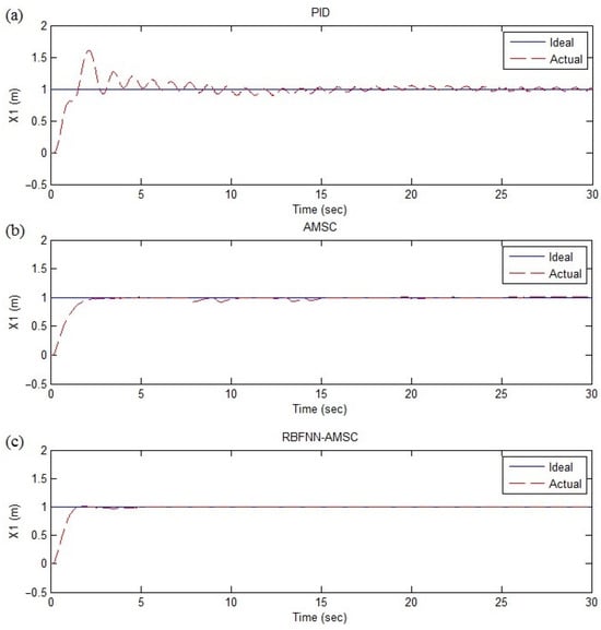
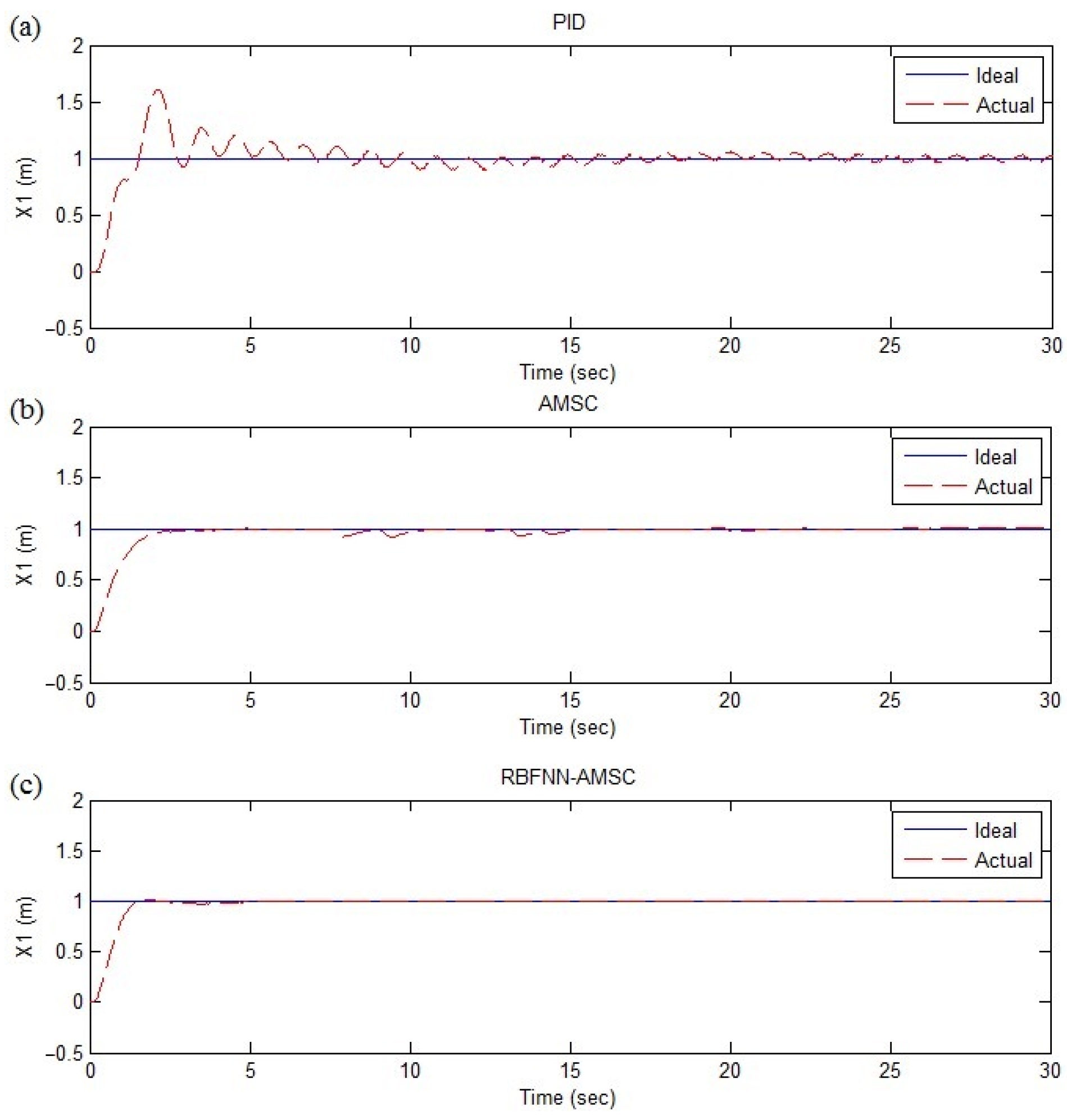
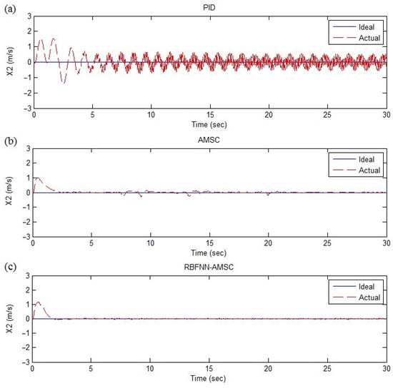
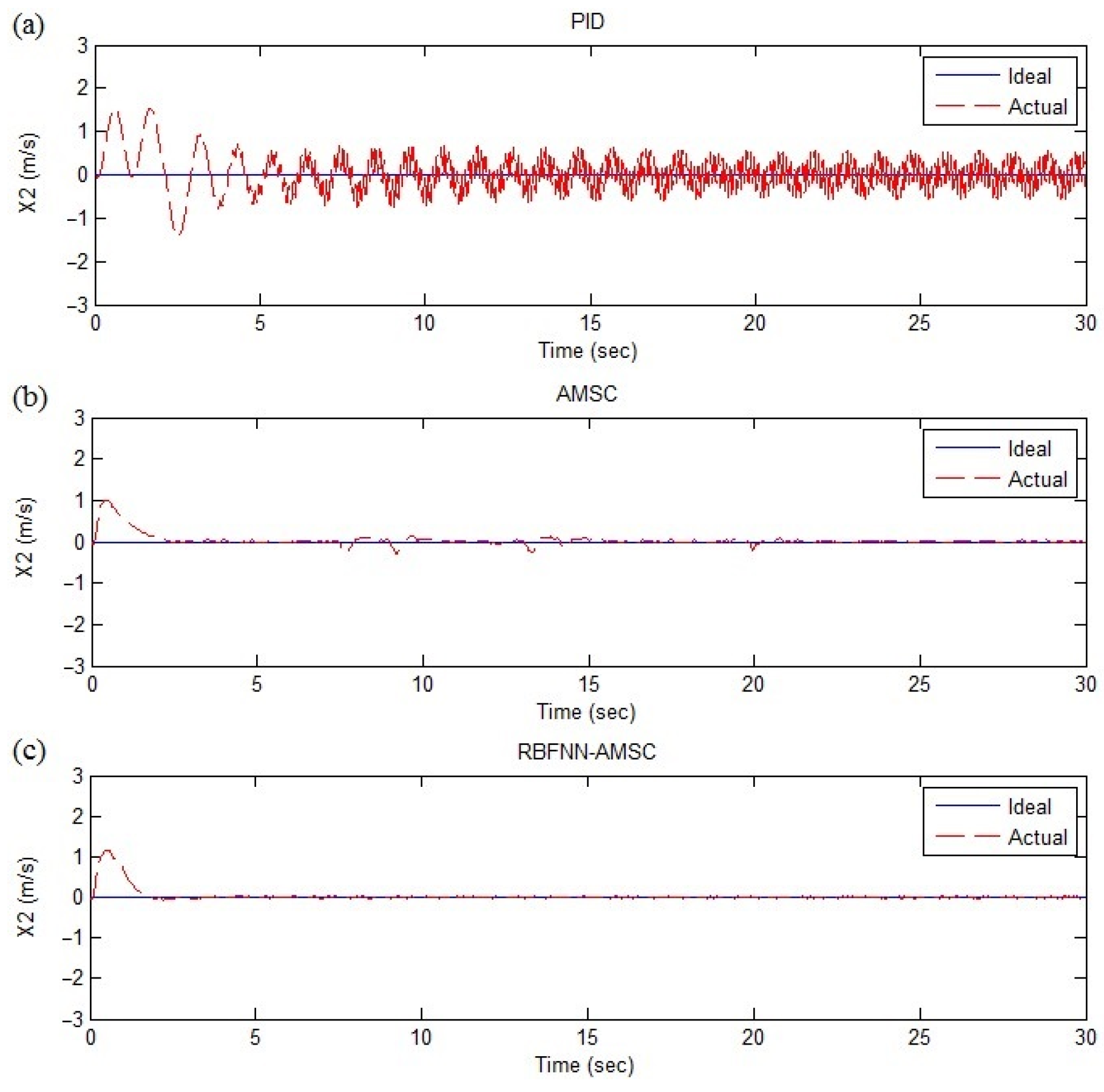
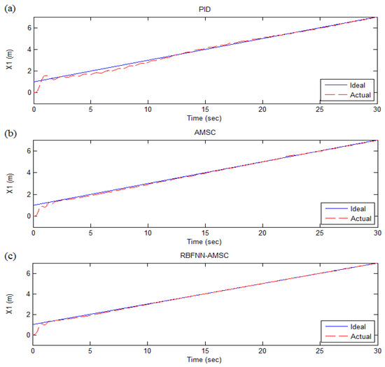
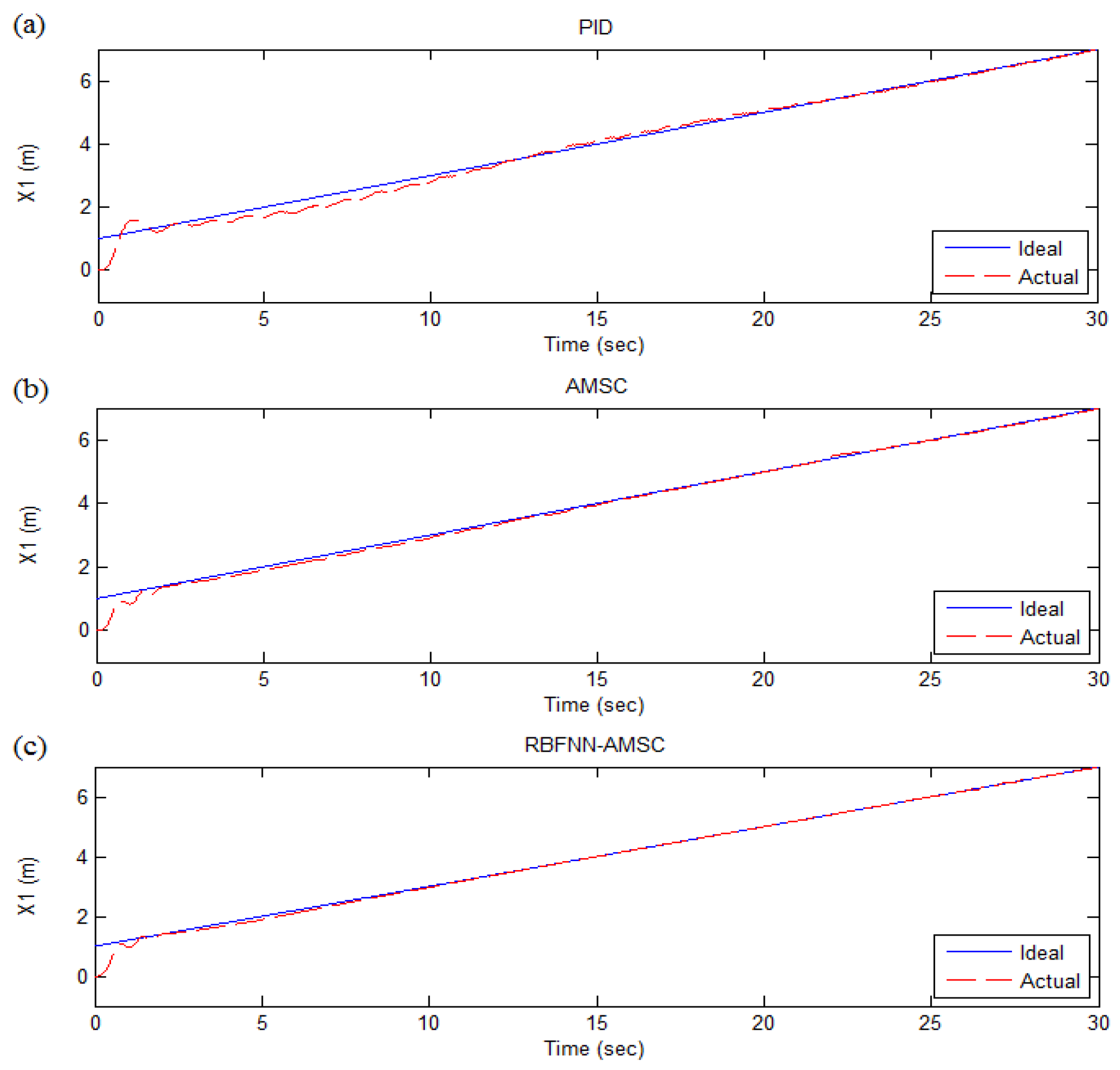
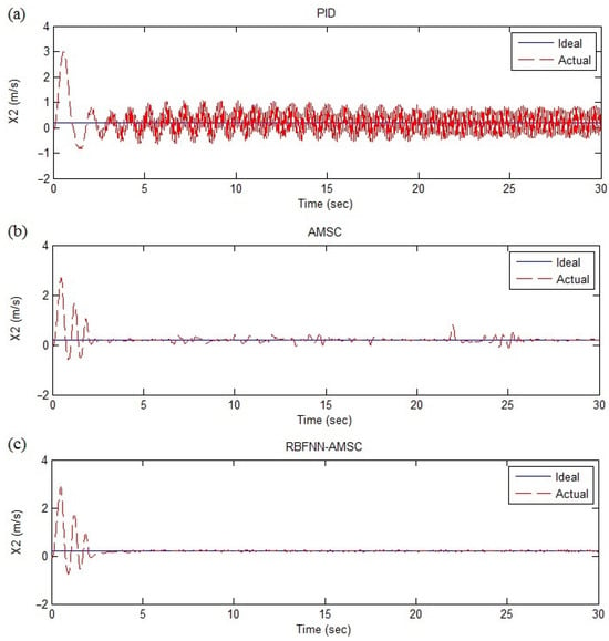
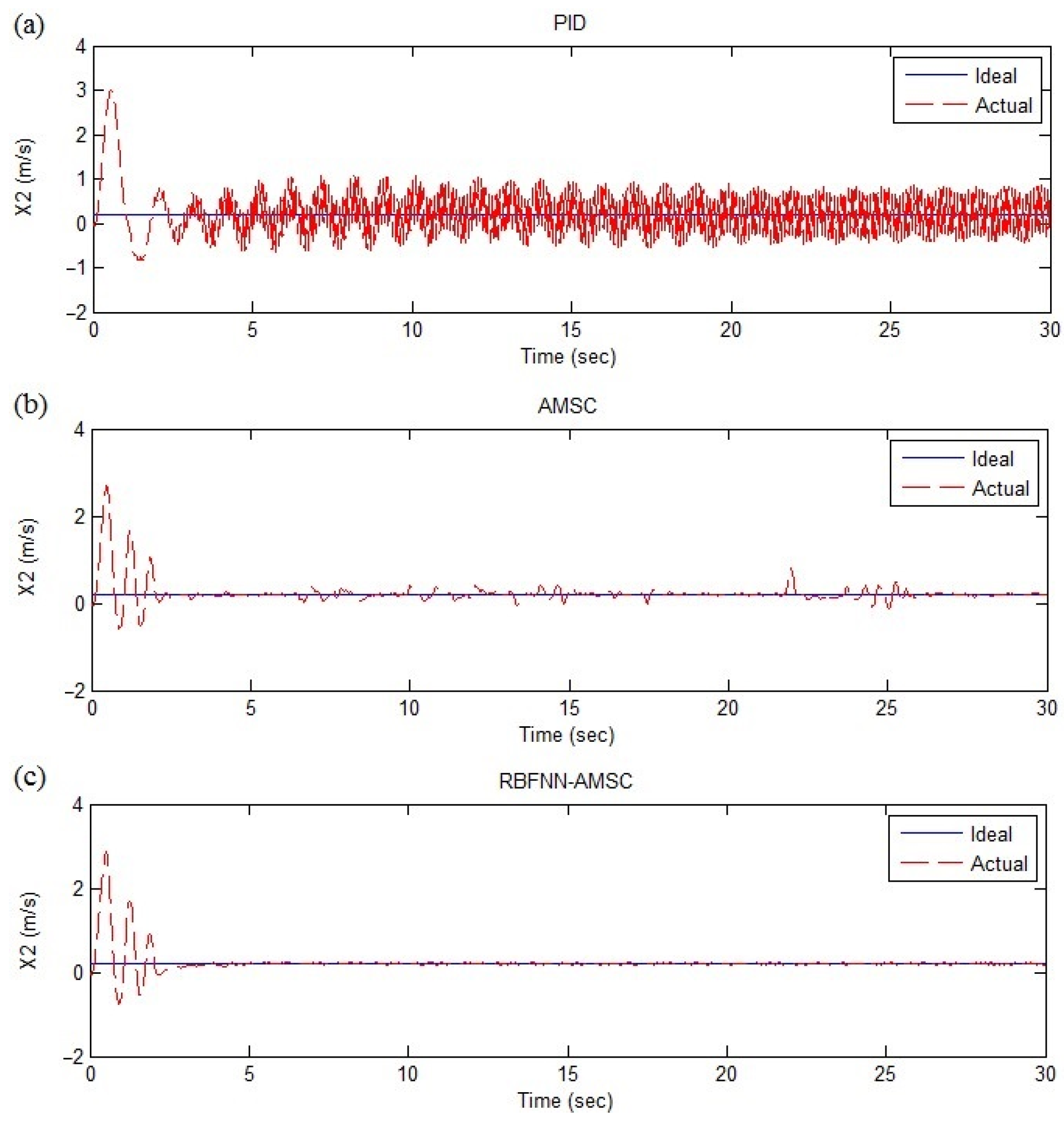
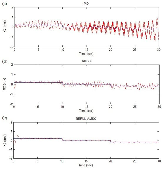
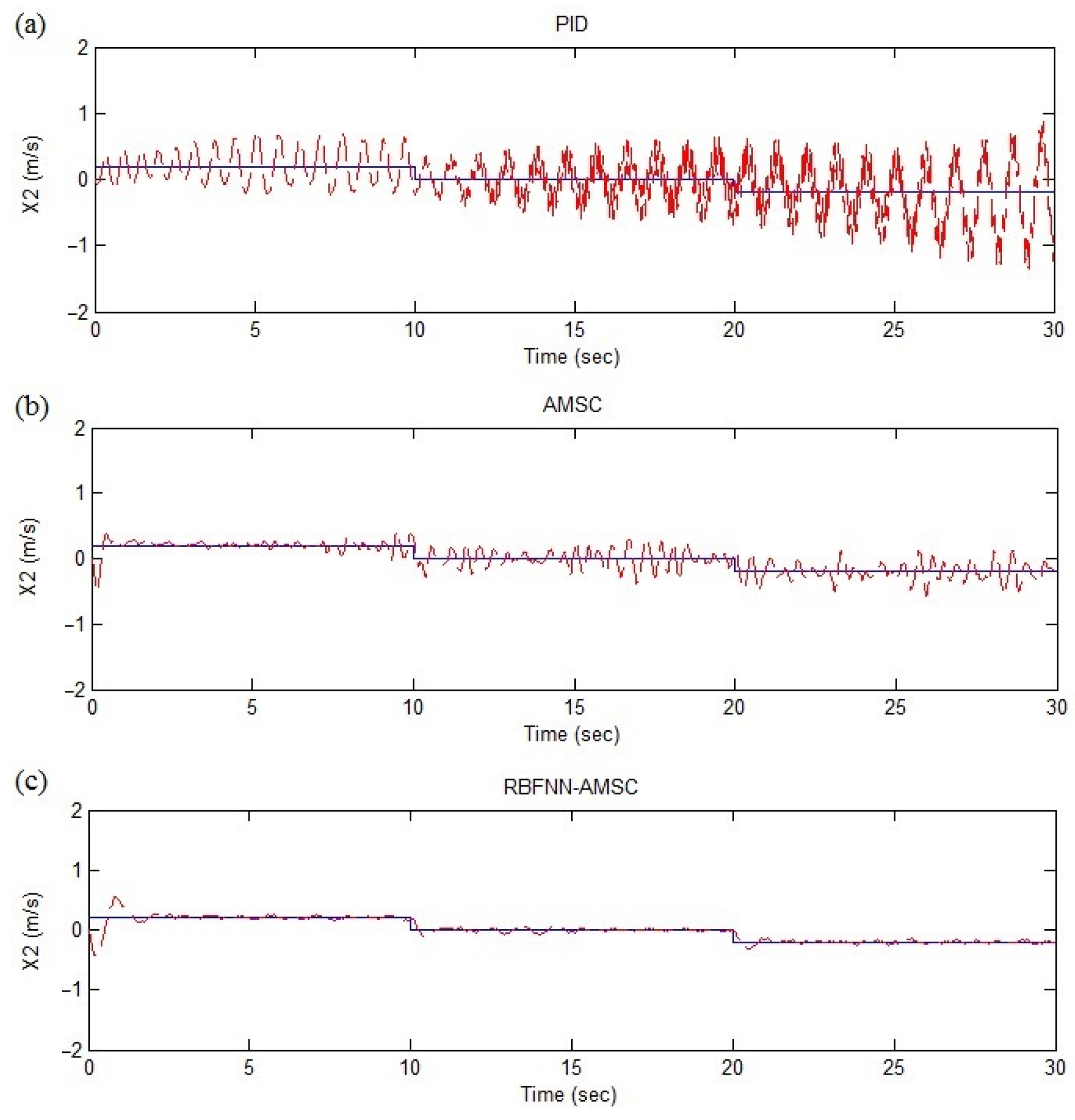
The state responses of and in constant displacement tracking are shown in Figure 4 and Figure 5, and the simulation data in steady state are analyzed in Table 3. In Figure 4, significant vibration is observed in the transient phase for PID control, and low-amplitude oscillations are still present in the steady state. AMSC performs better, but low-frequency oscillations also occur in the steady state. On the other hand, RBFNN-AMSC drives the underwater vehicle smoothly along the ideal trajectory without oscillations. A similar phenomenon can be observed in Figure 5, which can also be confirmed through the data comparison in Table 3. In addition, the oscillations in Figure 5 are more aggravated than in Figure 4, especially for the PID control performance, which means although the PID controller can achieve required displacement tracking control with oscillations, the state response of is unsatisfactory. Therefore, from the aforementioned simulation results, we may draw a conclusion that the performance of RBFNN-AMSC in constant displacement tracking of case 1 is better than the PID controller and conventional AMSC.
Figure 4.
State responses of in constant displacement tracking in case 1. (a) PID control performance; (b) AMSC performance; (c) RBFNN-AMSC performance.
Figure 5.
State responses of in constant displacement tracking in case 1. (a) PID control performance; (b) AMSC performance; (c) RBFNN-AMSC performance.
Table 3.
The comparison of simulation results of constant displacement tracking in case 1.
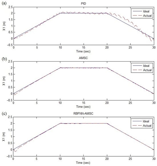
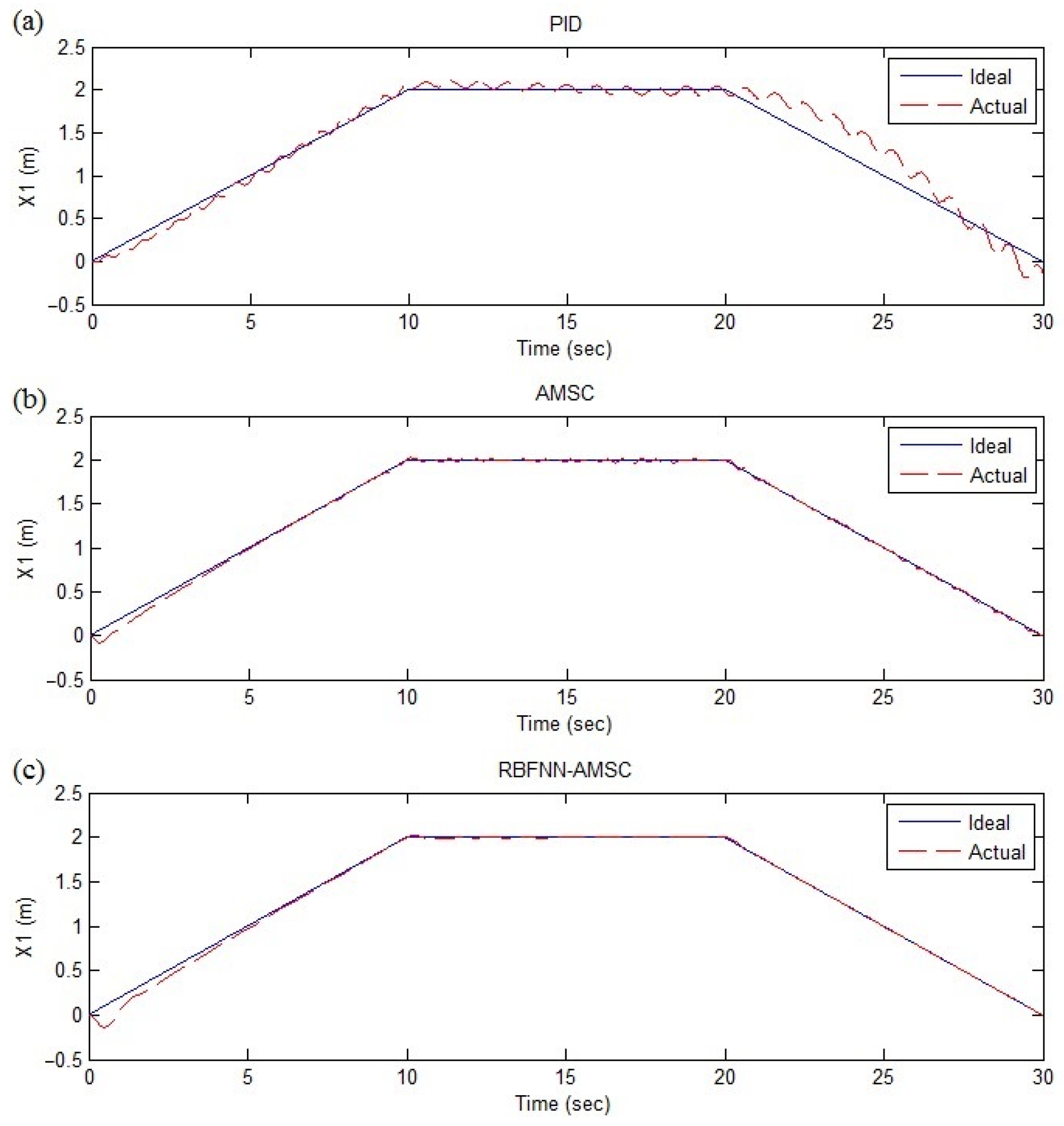
The state responses of and in ramp displacement trajectory tracking are presented in Figure 6 and Figure 7, and the simulation data in steady state are analyzed in Table 4. The simulation results also show that RBFNN-AMSC performs better than the PID controller and conventional AMSC in tracking precision and stability. In addition, a slight increase in average steady-state errors can be observed in ramp displacement tracking compared to constant displacement tracking.
Figure 6.
State responses of in ramp displacement tracking in case 1. (a) PID control performance; (b) AMSC performance; (c) RBFNN-AMSC performance.
Figure 7.
State responses of in ramp displacement tracking in case 1. (a) PID control performance; (b) AMSC performance; (c) RBFNN-AMSC performance.
Table 4.
The comparison of simulation results of ramp displacement tracking in case 1.
To further verify the adaptability of the proposed approach, a combined curve is selected as the ideal displacement trajectory, which is actually the combination of a constant curve and ramp curve. The state responses of and in combined displacement trajectory tracking are shown in Figure 8 and Figure 9, and the simulation data in steady state are analyzed in Table 5. Similar conclusions can be drawn from the simulation results. In addition, compared with constant displacement tracking and ramp displacement tracking, the steady-state errors and oscillations of and here are larger, especially for the PID control performance, which means that, as the complexity of the ideal displacement trajectory increases, the superiority of RBFNN-AMSC is more distinct.
Figure 8.
State responses of in combined displacement tracking in case 1. (a) PID control performance; (b) AMSC performance; (c) RBFNN-AMSC performance.
Figure 9.
State responses of in combined displacement tracking in case 1. (a) PID control performance; (b) AMSC performance; (c) RBFNN-AMSC performance.
Table 5.
The comparison of simulation results of combined displacement tracking in case 1.
4.3. Case 2: Simulation with Time-Varying and State-Dependent Disturbance
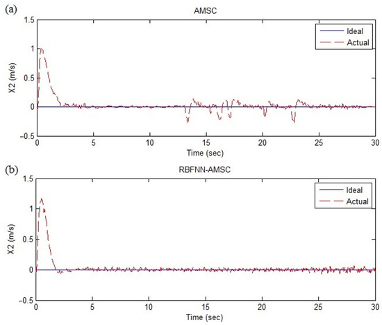
In case 2, the trajectory tracking simulations are carried out with time-varying and state-dependent disturbances . Compared with case 1, the upper bounds of disturbances used in case 2 are unknown. Since significant vibrations and steady-state errors occur in the performance of PID control in case 1, only conventional AMSC performances will be given for comparison in this case. In addition, the adaptabilities of RBFNN-AMSC and AMSC to different ideal curves have already been proved by simulation in case 1; to avoid repetition, only a constant curve is selected as the ideal displacement trajectory in case 2.
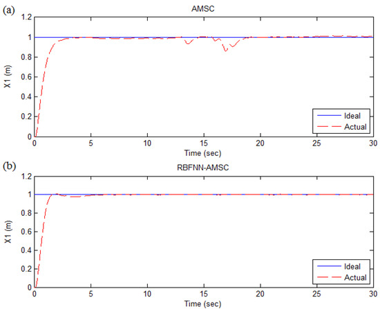
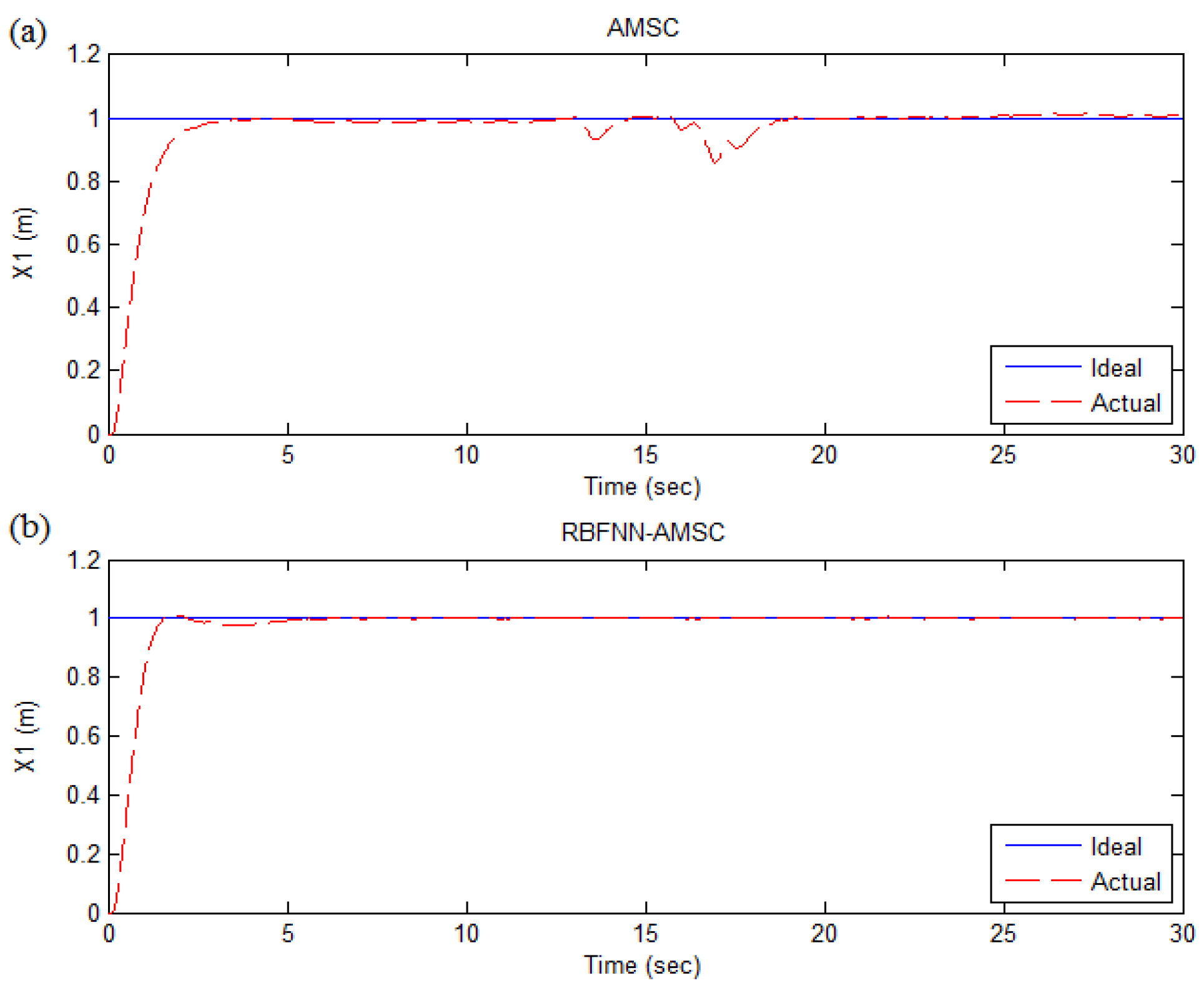
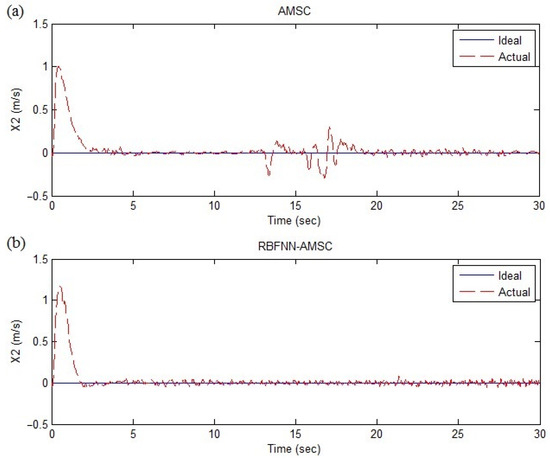
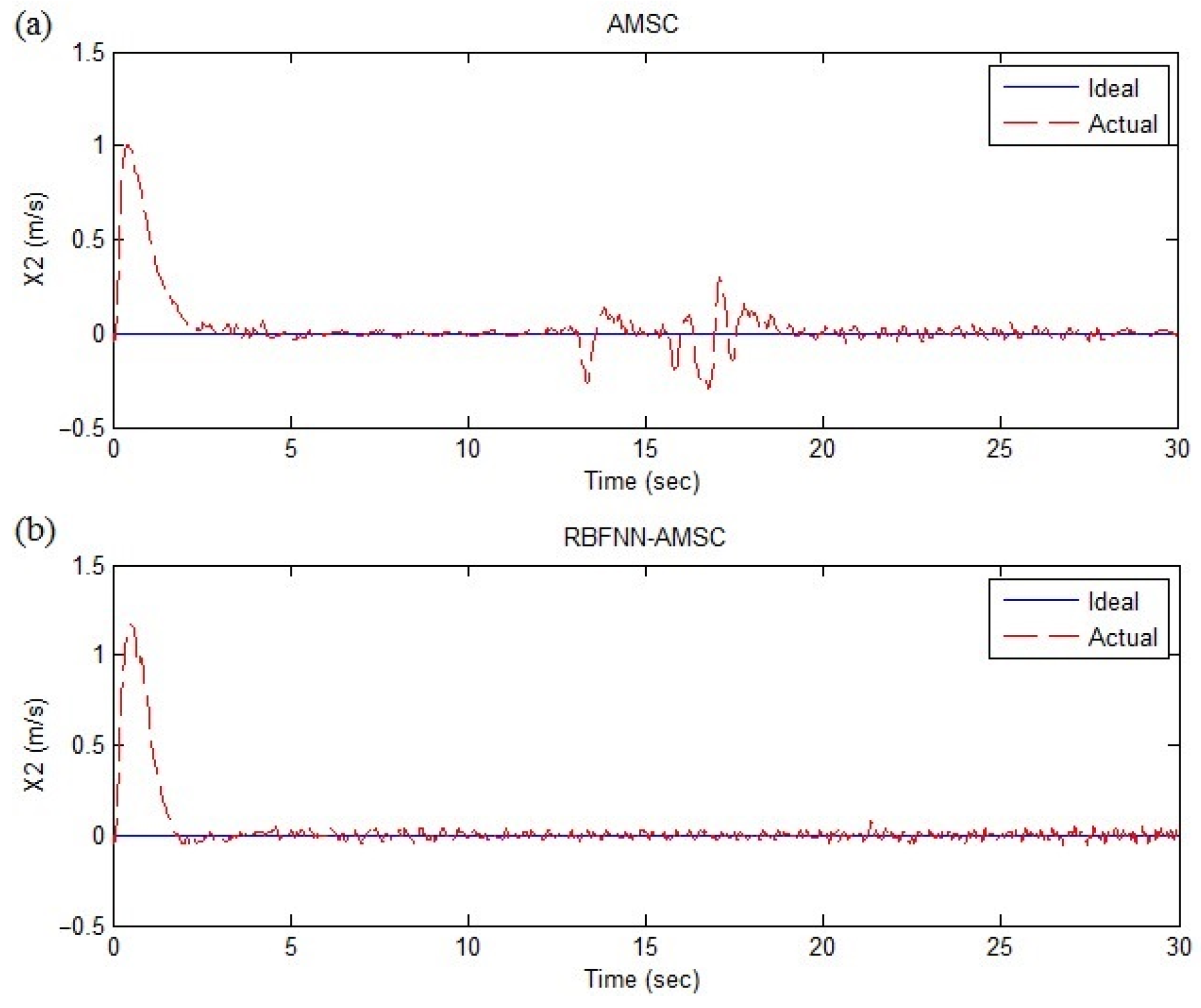
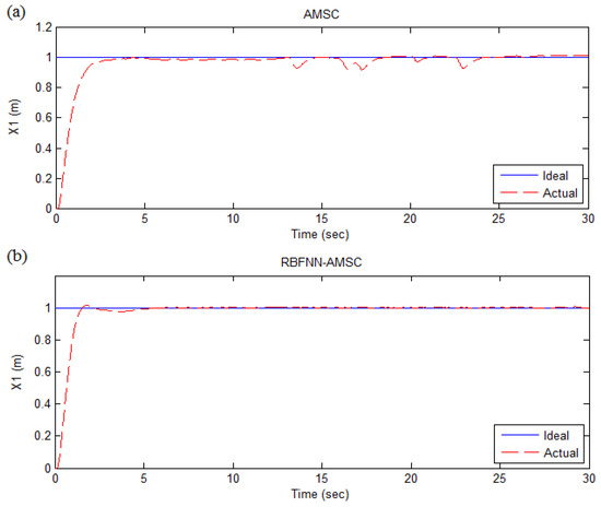
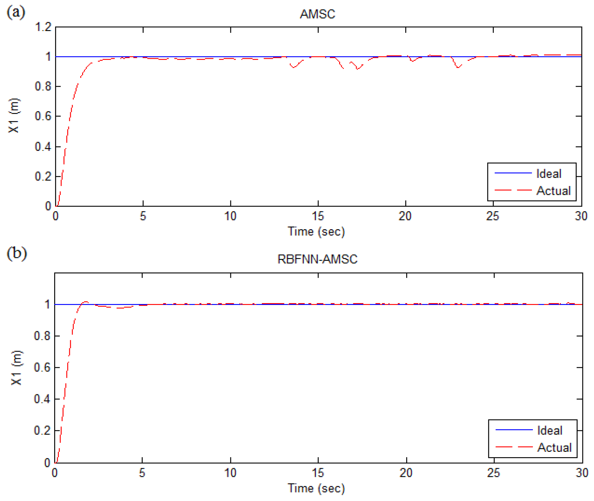
The state responses of and in case 2 are shown in Figure 10 and Figure 11, and the simulation data in steady state are analyzed in Table 6. Compared with conventional AMSC, the proposed controller performs better with smaller steady-state error and smaller oscillations in the state responses of both and . Besides, compared with case 1, great changes occur in the performance of conventional AMSC with bigger steady-state error and more oscillations, whereas the performance of the proposed controller has barely changed. The simulation results prove that the proposed controller has better anti-jamming capability than conventional AMSC when dealing with compound disturbances with unknown upper bounds, which mainly benefits from the superior disturbance estimation ability of RBFNN.
Figure 10.
State responses of in constant displacement tracking in case 2. (a) AMSC performance; (b) RBFNN-AMSC performance.
Figure 11.
State responses of in constant displacement tracking in case 2. (a) AMSC performance; (b) RBFNN-AMSC performance.
Table 6.
The comparison of simulation results of constant displacement tracking in case 2.
4.4. Case 3: Simulation with Piecewise Time-Varying and State-Dependent Disturbance
In case 3, the trajectory tracking simulations are carried out with piecewise time-varying and state-dependent disturbances, which can be described as . Compared with case 1 and case 2, the disturbances in case 3 are further upgraded since they have not only unknown upper bounds but also mutation characteristics. Similar to case 2, only constant displacement tracking will be carried out, with performances of the conventional AMSC and proposed controller presented for comparison.
The state responses of and in case 3 are shown in Figure 12 and Figure 13, and the simulation data in steady state are analyzed in Table 7. It is seen that compared with case 1 and case 2, the performance of conventional AMSC becomes worse with bigger steady-state error and more oscillations, especially when the amplitudes of compound disturbances suddenly increase after 15s, whereas the performance of the proposed controller has barely changed, which proves that the proposed controller has better anti-jamming capability to deal with suddenly changed disturbances.
Figure 12.
State responses of in constant displacement tracking in case 3. (a) AMSC performance; (b) RBFNN-AMSC performance.
Figure 13.
State responses of in constant displacement tracking in case 3. (a) AMSC performance; (b) RBFNN-AMSC performance.
Table 7.
The comparison of simulation results of constant displacement tracking in case 3.
4.5. Simulation Results Summarization and Discussion
The aforementioned three simulation cases demonstrate the performance of the PID controller, AMSC, and proposed controller when confronting different kinds of disturbances.
In case 1, three different curves are selected as the ideal displacement trajectories to verify the adaptability of the controllers in different working conditions. Although the steady-state errors of the three controllers all increase as the ideal displacement curve becomes more complex, it is clearly seen that the performance of the proposed controller is better than the PID controller and conventional AMSC, with higher precision and less vibration, which can be proved by the curves and data. Taking as an example, the average of PID control in case 1 is 0.0801, whereas the average of AMSC is 0.0362, and the average of the proposed controller is 0.0173.
Since significant vibrations and steady-state errors have been observed in the PID control of case 1, and the adaptabilities to different working conditions have been proved, to avoid repetition, only the constant curve is selected as the ideal displacement trajectory in case 2 and case 3, and only the performance of AMSC will be presented for comparison. The simulation results show that as compound disturbances become more complex, the performance of conventional AMSC becomes worse with bigger steady-state error and more oscillations, whereas the performance of the proposed controller has barely changed. Taking as an example, compared with case 1, the of AMSC in case 2 has increased by 0.021, the of AMSC in case 3 has increased by 0.030, whereas the of RBFNN-AMSC in case 2 has increased by 0.0001, the of RBFNN-AMSC in case 3 has increased by 0.0002. Therefore, it is proved that the proposed controller has better anti-jamming capability to deal with various unknown disturbances.
From the aforementioned analyses, the following conclusion can be drawn: compared with the PID controller and conventional adaptive multiple-surface sliding controller, the proposed controller performs better with higher steady-state precision, smaller oscillation, and better capability of resisting disturbance.
However, this paper merely presents a preliminary exploration of the modeling and control algorithms for this new type of underwater vehicle, without verifying the effectiveness of the algorithms through actual experiments. Therefore, the algorithms also have certain limitations: in the current simulation, the parameters of the RBF neural network are selected using data obtained from previous simulations. Considering the inevitable differences between practical application scenarios and simulation scenarios, the existing RBFNN parameters may not be optimal. In practical applications, it is necessary to combine more experimental results to optimize the parameters of RBFNN and conduct sensitivity analysis, thereby obtaining optimal control parameters that are more in line with actual requirements.
5. Conclusions
The current work focuses on the modeling and controller design of an underwater cable-driven system, with the aim of accomplishing high-precision displacement tracking control. Considering the complex dynamic behavior and harsh underwater environment, a high-order nonlinear model with unknown matched and mismatched disturbances is obtained. Subsequently, considering the system characteristics and control objectives, a RBFNN based adaptive multiple-surface sliding control strategy is proposed. With estimation of matched and mismatched uncertainties achieved by an adaptive RBF neural network, the influences of unknown compound disturbances are compensated, and system anti-jamming capability is improved. Using backstepping design procedure and multiple-surface sliding control method, stability and robustness of the system are ensured. Meanwhile, by employing exponential reaching law design, the convergence rate of each subsystem is improved. Besides, the stability of the controller is proved by a Lyapunov approach. Simulation cases under different kinds of disturbances show the efficiency of the proposed design. However, this article only presents a preliminary study on this type of underwater vehicle, with limited refinement in modeling and optimization of algorithms. In the future, further optimization of algorithms will be conducted, and experimental verification will be carried out.
Author Contributions
Conceptualization, K.X. and Y.X.; methodology, K.X.; software, K.X.; validation, K.X. and Y.X.; formal analysis, Y.X.; investigation, K.X.; resources, Y.X.; data curation, K.X.; writing—original draft preparation, K.X.; writing—review and editing, Y.X.; visualization, K.X.; supervision, Y.X.; project administration, Y.X.; funding acquisition, Y.X. All authors have read and agreed to the published version of the manuscript.
Funding
This work was supported by the National Natural Science Foundation of China (52001132), Special Funds for Basic Scientific Research in Central Universities of China (2662025GXPY008), and the Foundation of Hubei Province Key Laboratory for Unmanned Underwater Vehicle and Manipulating Technology, Huazhong University of Science and Technology (Grant No. CHK202401).
Data Availability Statement
The original contributions presented in this study are included in the article. Further inquiries can be directed to the corresponding author.
Conflicts of Interest
The authors declare no conflict of interest.
References
- Wibisono, A.; Piran, M.J.; Song, H.-K.; Lee, B.M. A Survey on Unmanned Underwater Vehicles: Challenges, Enabling Technologies, and Future Research Directions. Sensors 2023, 23, 7321. [Google Scholar] [CrossRef] [Scilit] [PubMed]
- Ravichandran, R.; Umapathy, A.; Babu, S.M.; Vedhachalam, N.; Venkatesan, K.; Harikrishnan, G.; Subramanium, A.; Ramadass, G.; Atmanand, M. Heat dissipation studies on sub- sea cables wound on winches. In Proceedings of the 2015 IEEE Underwater Technology (UT), Chennai, India, 23–25 February 2015; pp. 1–4. [Google Scholar]
- Cao, Y.; Yu, C.; Xu, C.; Xiang, X.; Lian, L. MORSE: A Rapid Marine Organism Observation Framework via Sonar Point Map. IEEE J. Ocean. Eng. 2026, 51, 2222–2241. [Google Scholar] [CrossRef] [Scilit]
- Chen, K.; Chen, Z.; Yu, J.; Ren, K.; Jiao, W.; Chen, K.; Tian, Y.; Sun, J. A hybrid data-driven and physical model-based approach for predicting the mechanical properties of cable-arrays in flexible cable dual-AUVs systems. Ocean Eng. 2025, 329, 121099. [Google Scholar] [CrossRef] [Scilit]
- Xia, Y.; Xu, G.; Xu, K.; Chen, Y.; Xiang, X.; Ji, Z. Dynamics and control of underwater tension leg platform for diving and leveling. Ocean Eng. 2015, 109, 454–478. [Google Scholar] [CrossRef] [Scilit]
- Petritoli, E.; Leccese, F. Towed Underwater Drones: Main Operative Problems and Analysis of Longitudinal Stability. In Proceedings of the 2024 IEEE International Workshop on Metrology for the Sea; Learning to Measure Sea Health Parameters (MetroSea), Portorose, Slovenia, 14–16 October 2024; pp. 454–458. [Google Scholar]
- Conte, G.; Serrani, A.; Perdon, A.M. Rejecting the disturbances due to the umbilical’s traction in ROV’s control. In Proceedings of the IEEE Oceanic Engineering Society. OCEANS’98. Conference Proceedings (Cat. No.98CH36259), Nice, France, 28 September–1 October 1998; pp. 1245–1248. [Google Scholar]
- Feng, H.; Sun, W.; Tang, G.; Wang, J.-J. Study on a novel two-part underwater towed system for near-surface towed vehicle test. Ocean Eng. 2022, 255, 111440. [Google Scholar] [CrossRef] [Scilit]
- Li, Y.; Sadeghian, H.; Forouhar, M.; Naceri, A.; Haddadin, S. Distributed modeling and torque transmission analysis of a cable-driven robotic joint. Mechatronics 2026, 117, 103517. [Google Scholar] [CrossRef] [Scilit]
- Li, J.; Li, Y. Inverse kineto-static modelling and analysis of suspended cable-driven parallel robots based on elastic catenary theory. Robot. Auton. Syst. 2026, 204, 105558. [Google Scholar] [CrossRef] [Scilit]
- Tan, K.; Shi, H.; Mei, X.; Geng, T.; Yang, J. Control of force transmission for cable-driven actuation system based on modified friction model with compensation parameters. Control Eng. Pract. 2024, 151, 106035. [Google Scholar] [CrossRef] [Scilit]
- González-Carbajal, J. An analytical model for the drum-rope interaction in hoisting mechanisms and cable-driven systems. Mech. Mach. Theory 2025, 207, 105939. [Google Scholar] [CrossRef] [Scilit]
- Luo, X.; He, S. Dynamic Modeling and Simulation of a Cyclic Towing System for Underwater Vehicles. Appl. Sci. 2024, 14, 10767. [Google Scholar] [CrossRef] [Scilit]
- Kim, H.-G.; Yun, S.-J.; Park, J.-W.; Lee, H.-J.; Hwang, J.-H.; Kim, J.-C.; Choi, Y.-H.; Ryu, J.-K.; Suh, J.-H. Estimation and Control of a Towed Underwater Vehicle with Active Stationary and Low-Speed Maneuvering Capabilities. J. Mar. Sci. Eng. 2023, 11, 1176. [Google Scholar] [CrossRef] [Scilit]
- Minowa, A.; Toda, M. Stability analyses on a towed underwater vehicle motion control system using a high-gain observer. Adv. Control Appl. Eng. Ind. Syst. 2021, 3, e77. [Google Scholar] [CrossRef] [Scilit]
- Mahapatra, S.; Subudhi, B.; Rout, R.; Kumar, B.K. Nonlinear H∞ control for an autonomous underwater vehicle in vertical plane. IFAC-PapersOnLine 2016, 49, 391–395. [Google Scholar] [CrossRef] [Scilit]
- Glushchenko, A.; Lastochkin, K. Estimation of unknown values of known nonlinear mappings in adaptive control tasks. Eur. J. Control 2026, 89, 101489. [Google Scholar] [CrossRef] [Scilit]
- Shen, J.; Pan, Q.; Su, W.; Cui, Y.; Wang, H. Finite-time adaptive non-singular integral sliding mode control with saturation suppression for robotic manipulators. J. Frankl. Inst. 2026, 363, 108793. [Google Scholar] [CrossRef] [Scilit]
- Song, W.; Zuo, Y.; Tong, S. Inverse Q-learning optimal control for Takagi-Sugeno fuzzy unmanned surface vehicle systems. Inf. Sci. 2025, 721, 122600. [Google Scholar] [CrossRef] [Scilit]
- Yan, Z.; Lai, X.; Meng, Q.; Wu, M.; She, J.; Iwasaki, M. Modeling, analysis, and adaptive neural modified-backstepping control of an uncertain horizontal pendubot with double flexible joints. Control Eng. Pract. 2023, 139, 105647. [Google Scholar] [CrossRef] [Scilit]
- Oghabi, E.; Moghaddam, R.K.; Kobravi, H.R. Adaptive interval type-2 fuzzy neural network nonsingular fast terminal sliding mode control for cable-driven parallel robots. Eng. Appl. Artif. Intell. 2024, 136, 108963. [Google Scholar] [CrossRef] [Scilit]
- Pei, T.; Yu, C.; Zheng, J.; Zhang, H.; Cao, J.; Xiang, X.; Lian, L. Interpretable machine learning approach for AUV motion prediction based on lake-test data. J. Ocean Eng. Sci. 2025, 11, 180–190. [Google Scholar] [CrossRef] [Scilit]
- Huo, Z.; Liu, Z.; Li, J.; Wang, S.; Zhang, C.; Wang, J.; Han, G.; Chen, H.; Sun, Y. A novel combination of fixed-time extended state observer and adaptive super-twisting sliding mode controller for cable-driven wave motion compensation device. Ocean Eng. 2026, 355, 125215. [Google Scholar] [CrossRef] [Scilit]
- Ginoya, D.; Shendge, P.D.; Phadke, S.B. Sliding Mode Control for Mismatched Uncertain Systems Using an Extended Disturbance Observer. IEEE Trans. Ind. Electron. 2014, 61, 1983–1992. [Google Scholar] [CrossRef] [Scilit]
- Li, R.; Chen, M.; Wu, Q. Adaptive neural tracking control for uncertain nonlinear systems with input and output constraints using disturbance observer. Neurocomputing 2017, 235, 27–37. [Google Scholar] [CrossRef] [Scilit]
- Zou, X.; Zhang, L.; Zhong, P.; Meng, D.; Sun, H.-J.; Liu, Y.; Liu, W. Predefined-time trajectory tracking control of a rigid-flexible cable-driven space manipulator using neural network. Aerosp. Sci. Technol. 2026, 168, 111281. [Google Scholar] [CrossRef] [Scilit]
- Zhang, M.; Chen, Y.; Gao, Y.; Zhang, Y.; Zhang, Y. Adaptive sliding mode tracking and disturbance rejection control for cable-driven continuum robots in endoscopic surgery. Control Eng. Pract. 2026, 168, 106684. [Google Scholar] [CrossRef] [Scilit]
- Ding, L.; Yao, Y.; Lu, M.; Li, Y.; Wang, Y. Integration of linear extended state observer within proxy-based sliding mode control for a cable-driven aerial manipulator. Robot. Auton. Syst. 2025, 194, 105161. [Google Scholar] [CrossRef] [Scilit]
- Aghaseyedabdollah, M.; Abedi, M.; Pourgholi, M. Interval type-2 fuzzy sliding mode control for a cable-driven parallel robot with elastic cables using metaheuristic optimization methods. Math. Comput. Simul. 2024, 218, 435–461. [Google Scholar] [CrossRef] [Scilit]
- Ginoya, D.; Shendge, P.; Phadke, S. Disturbance observer based sliding mode control of nonlinear mismatched uncertain systems. Commun. Nonlinear Sci. Numer. Simul. 2015, 26, 98–107. [Google Scholar] [CrossRef] [Scilit]

Disclaimer/Publisher’s Note: The statements, opinions and data contained in all publications are solely those of the individual author(s) and contributor(s) and not of MDPI and/or the editor(s). MDPI and/or the editor(s) disclaim responsibility for any injury to people or property resulting from any ideas, methods, instructions or products referred to in the content. |
© 2026 by the authors. Licensee MDPI, Basel, Switzerland. This article is an open access article distributed under the terms and conditions of the Creative Commons Attribution (CC BY) license.