


Abstract
Lane keeping under degraded visual confidence remains challenging because most existing approaches focus either on improving lane-feature extraction or on estimating vehicle motion, while giving less attention to how unreliable visual measurements should modify the estimator–controller interaction in a physical closed-loop system. This paper presents a confidence-gated Kalman lane-keeping architecture for a 1:10-scale autonomous vehicle. The methodological contribution lies in the direct coupling of visual confidence, state estimation, and steering control: unreliable lane measurements are down-weighted through confidence-dependent measurement noise, while the propagated lane-relative state remains available to the controller. The primary experimental unit is the run, defined as one logged lap under one control configuration; frame-level summaries are retained only as historical reproducibility material. In the run-level comparison, the autonomous vision, inertial measurement unit (IMU)-feedforward, and Kalman filter (KF) group KF_G1—the first inferential KF generation—had lower mean absolute error than the human baseline, while vision and KF_G1 had overlapping run-level confidence intervals for absolute error. KF_G1 shifted the mean signed bias closer to the lane reference than the vision and IMU groups, but with higher run-level spread than vision. KF_G2, the second observational KF generation, is reported only as an observational generation comparison, so no causal claim is made for its estimator–controller correction weight setting. KF_G3, the single descriptive adverse-condition KF run, is reported without an estimable confidence interval or population-level adverse-illumination inference. A further limitation is that the inertial prediction pathway was inactive in the logged Kalman-filter runs because the inertial coupling coefficient . The main contribution is a reproducible run-level evaluation of confidence-gated estimator–controller coupling that distinguishes supported evidence from observational and descriptive cases.
1. Introduction
In the lane-keeping experiment reported here, the closed-loop control system depends on a simple but fragile quantity: the lateral error inferred from the visible lane geometry. When that measurement is available, a camera-based controller can run with modest hardware and without external positioning. When the lane cue is degraded, however, the steering command is affected immediately because the controller no longer receives a reliable lane-relative feedback signal. This problem is well known in larger autonomous-navigation settings, where road perception becomes difficult when sensors must operate without additional positioning information [1], and where continuous state information is needed for navigation and control [2,3].
The specific failure mode studied in this work is loss of visual reliability under adverse illumination. Illumination changes, shadows, low texture, motion blur, sharp turns, partial occlusions, and dynamic objects can reduce the reliability of visual odometry, visual tracking, or lane-feature extraction [2,3,4]. Indoor visual simultaneous localization and mapping (SLAM) studies also show that illumination variation alone can cause relocalization failures when a robot relies only on camera-based perception [5]. In a lane-keeping loop, the same issue appears as intermittent or unreliable lateral-error measurements: lane markings may become poorly contrasted, overexposed, underexposed, or temporarily unobservable. From an automation perspective, visual degradation becomes critical when it interrupts the feedback signal required by the lateral controller. What matters for this controller, then, is less the per-frame detection accuracy and more whether a usable lane-relative state survives the frames where that confidence drops.
On this vehicle, the IMU does not replace the camera; it fills a narrower gap in the camera-to-control stream. Lane position still has to come from the image, since integrating angular-rate data alone drifts and carries no information about where the lane actually is. What the 50 Hz yaw-rate stream offers instead is a motion cue indifferent to lighting and contrast—the same complementary role that IMU data play in visual–inertial estimation, where they support motion tracking, scale recovery, and bridging the short visual outages caused by illumination changes, textureless regions, or motion blur [2,4]. The present setup keeps that idea narrow: trust the camera when the lane fit is good, and fall back on prediction only to keep the lateral state alive when visual confidence drops.
A Kalman filter fits this logic directly: it already separates prediction from update, so confidence gating only has to act on the update half of the cycle. Related visual–inertial work has used the extended Kalman filter (EKF), the iterated EKF (IEKF), the error-state Kalman filter (ESKF), and the multi-state constraint Kalman filter (MSCKF) for pose estimation, odometry, and localization [3,4,6,7]. Those studies guided the estimator choice, but their usual performance target was different from the one tested here. In this manuscript, the state estimate is sent directly to the steering controller. A loss of visual confidence is therefore not only an estimator event; it is a control-loop event that can change the steering command and the continuity of the lane-keeping function.
Lane-perception studies also report that single-frame or single-sensor processing can be insufficient for lane-related estimation [1,8]. The remaining issue for this experiment is what happens after the detector becomes uncertain. Improving the lane extractor is important, but the controller still needs a lateral-error signal when the extractor reports low confidence. That downstream estimator–controller behavior is the part isolated in the experiments below.
Existing lane-perception studies primarily seek to improve lane-marker extraction, segmentation accuracy, or robustness to illumination changes, whereas visual–inertial estimation studies commonly focus on pose, odometry, or localization accuracy. Comparatively less attention has been given to the control-level consequence of unreliable lane measurements when the estimated lateral state is used directly as feedback for physical steering. The unresolved problem addressed here is therefore not only whether lane features can be detected under degraded illumination but how visual confidence should modify the estimator update and the controller input when those measurements become temporarily unreliable.
The methodological novelty of this work does not lie in the isolated use of bird’s-eye-view transformation, temporal heatmap accumulation, Random Sample Consensus (RANSAC) fitting, Kalman filtering, or proportional–derivative (PD) steering control, all of which are established techniques. The contribution lies in their confidence-aware closed-loop integration: visual reliability directly modulates the Kalman measurement update, the propagated lane-relative state is coupled with the steering command, and the resulting behavior is evaluated on a physical vehicle using the experimental run as the primary unit of analysis. The inertial branch remains architecturally present in the estimator formulation, but it was inactive during the reported Kalman-filter runs because the inertial coupling coefficient , so the confidence-aware coupling demonstrated here is evaluated under kinematic state propagation rather than calibrated visual–inertial fusion.
This paper therefore reports a run-level evaluation of a confidence-gated Kalman lane-keeping architecture on a 1:10-scale autonomous vehicle under controlled indoor conditions. The camera pipeline provides the primary lane-relative measurement, while the estimator includes an inertial prediction pathway intended to use yaw-rate information when calibration is available. The experiments compare vision-only lane keeping, IMU-assisted feedforward compensation, and the Kalman control architecture with confidence-gated visual updates, including favorable runs and a single descriptive adverse-condition Kalman run. The purpose is deliberately limited: the work does not claim that calibrated IMU prediction universally reduces average tracking error, but it examines whether confidence-gated Kalman propagation can preserve operational continuity when visual lane cues become temporarily unreliable or unavailable. The main contributions of this work are summarized as follows:
- A confidence-aware estimator–controller architecture in which visual reliability directly modulates the Kalman measurement update and, therefore, the lane-relative feedback signal used for steering control.
- A closed-loop integration strategy that couples perception confidence, temporal state propagation, and PD steering correction to preserve a usable controller input during temporary degradation of visual lane measurements.
- A reproducible run-level evaluation framework that distinguishes inferential, observational, and descriptive evidence across vision-only, IMU-feedforward, Kalman-filter, and human-reference configurations, while explicitly documenting that the inertial prediction term was inactive in the reported Kalman runs because .
2. Related Work
2.1. Vision-Based Lane Perception Under Challenging Conditions
Vision-based lane perception remains one of the most widely used approaches for lane keeping and autonomous driving because cameras provide dense geometric and appearance information at relatively low cost. Surveys on lane detection have shown that both classical and deep-learning-based methods have advanced substantially, but robust performance remains difficult under non-uniform illumination, shadows, occlusions, worn lane markings, and complex road appearances [9]. These challenges are directly relevant to closed-loop lane keeping because the controller depends not only on detecting lane markings but also on receiving temporally consistent and reliable lane-relative measurements.
Several works have specifically addressed visual degradation caused by shadows, occlusions, and illumination changes. Tapia-Espinoza and Torres-Torriti proposed a robust lane-sensing and lane-departure-warning system designed to operate under shadows and partial occlusions [10]. Hoang et al. addressed shadow-robust lane detection using a visible-light camera and a fuzzy-system-based approach [11]. More recently, Lee et al. improved lane-detection performance by integrating a camera with dual light sensors, explicitly considering difficult illumination scenarios such as backlight, tunnels, and night driving [12]. These studies demonstrate that illumination-aware processing can improve the reliability of lane perception; however, most of them focus on improving the perception module itself rather than evaluating how degraded lane measurements affect the continuity of a closed-loop lane-keeping controller.
Yordanov et al. pushed detection accuracy further with a deep-learning framework tuned jointly for lane detection and steering output [13]. A more accurate detector is still only as useful as the visual evidence it is given, though; once lane pixels become scarce or absent, accuracy gains on well-lit frames do not carry over. Vision remains the primary measurement source for lane keeping in this work as well, which leaves the same unresolved control question: what the controller is supposed to do once that measurement becomes intermittent under adverse illumination.
2.2. Visual–Inertial Estimation and Kalman-Based State Prediction
Visual–inertial fusion has become a consolidated strategy for robotic state estimation because cameras and inertial sensors provide complementary information. Cameras supply exteroceptive measurements related to scene geometry and visual features, whereas IMUs provide high-rate inertial measurements that are less sensitive to lighting and texture. VINS-Mono demonstrated the effectiveness of tightly coupled monocular visual–inertial estimation for robust six-degree-of-freedom state estimation [2]. Similarly, Bloesch et al. proposed an iterated extended Kalman filter for visual–inertial odometry using direct photometric feedback [4]. These methods provide strong evidence that visual and inertial information can be combined to improve state estimation, but their primary objective is odometry or pose estimation rather than lane-relative control.
Kalman-filter-based estimators have also been applied to mobile robots and ground vehicles. Alatise and Hancke used an extended Kalman filter to combine IMU and vision data for mobile-robot pose estimation [6]. Ma et al. proposed ACK-MSCKF, a tightly coupled Ackermann multi-state constraint Kalman filter for autonomous vehicle localization, showing the importance of incorporating ground-vehicle motion constraints in visual–inertial estimation [3]. Chen et al. developed a ToF visual–inertial odometry system for perception in dark GNSS-denied environments, further supporting the need for complementary sensing under degraded visual conditions [7]. Reviews on visual–inertial navigation and autonomous-vehicle state estimation also emphasize that robust estimation depends on managing the complementary strengths and weaknesses of sensing modalities [14,15].
Other recent works have extended multisensor estimation beyond camera–IMU pairs. Zhao et al. proposed an adaptive LiDAR–visual–inertial odometry system for agricultural unmanned ground vehicles, illustrating the relevance of adaptive multisensor estimation in complex outdoor environments [16]. Taken together, these studies show that visual–inertial and multisensor approaches are mature research directions for state estimation and localization. Nevertheless, their evaluation typically focuses on trajectory accuracy, localization drift, or odometry robustness. In contrast, the present work evaluates a task-oriented Kalman architecture whose estimated state is directly coupled with the lateral lane-keeping control loop.
2.3. Small-Scale Autonomous Vehicles for Control Validation
Small-scale autonomous vehicles provide a practical experimental platform for testing perception, control, and autonomy algorithms under controlled and reproducible conditions. The F1TENTH platform has been widely adopted as an open-source 1:10-scale environment for continuous control, reinforcement learning, and autonomous racing research [17]. More recent surveys and benchmarks on F1TENTH autonomous racing further highlight the importance of standardized small-scale platforms for comparing perception, planning, and control methods before deployment on full-size vehicles [18].
From a broader autonomous-driving perspective, motion planning and control surveys emphasize that autonomous navigation requires the coordination of perception, state estimation, planning, and low-level control [19,20]. However, many full-scale autonomous-driving studies focus on high-level planning, trajectory generation, or vehicle-control taxonomies rather than experimentally isolating how degraded perception affects a specific closed-loop lane-keeping function. Small-scale platforms are therefore especially useful for studying this interaction, because perception failures, controller responses, and estimator architectures can be evaluated repeatedly in a controlled environment.
The present experimental platform follows this philosophy by using a low-cost 1:10-scale autonomous vehicle to evaluate lane keeping under controlled illumination conditions. Unlike purely simulation-based studies or general autonomous-driving benchmarks, the proposed system couples an active-infrared lane-perception pipeline, an external IMU, and a Kalman-based confidence-gated state estimator within the actual steering-control loop. This enables the evaluation of motion-control continuity when the visual lane measurement becomes unreliable.
2.4. Automation-Oriented Positioning of the Present Work
The works closest to the present study combine lane perception with multisensor or temporal fusion. Li et al. proposed a drivable-region and lane-detection system based on feature-level fusion of LiDAR and vision for autonomous vehicle navigation in challenging road scenarios [1]. Sun et al. proposed a multi-stage Hough-space lane-marking detection method that combines IMU and vision information with Kalman filtering to improve the reliability of lane-marking detection across frames [8]. These studies demonstrate that single-sensor or single-frame perception can be insufficient for robust lane-related perception, and that additional sensing or temporal filtering can improve reliability.
Table 1 summarizes this positioning qualitatively against six representative studies already discussed above, spanning lane-perception, visual–inertial estimation, and small-scale closed-loop-control research. The comparison is necessarily qualitative: the compared studies evaluate heterogeneous outputs (detection accuracy, pose or trajectory error, localization drift, lap-time or control benchmarks) under different validation protocols, so their reported numbers are not directly comparable to the run-level lane-relative error reported in this manuscript and are not reproduced in the table. The table does not rank the compared approaches; its purpose is to show where the methodological difference of the present work lies—specifically, in treating perception confidence as a signal that directly regulates estimator–controller coupling in a physical steering loop—rather than to claim that the present work outperforms any of them on their own evaluation target.
Table 1.
Qualitative comparison of representative lane-perception, visual–inertial estimation, and closed-loop lane-keeping approaches. All six comparators are already discussed earlier in Section 2; no reference outside the manuscript’s existing bibliography was added for this comparison.
However, there remains a distinction between improving lane perception and evaluating the functional continuity of lane keeping. Most lane-perception studies assess detection accuracy, robustness to shadows, or reliability of lane-marker extraction, while most visual–inertial estimation studies assess pose estimation, odometry, or localization, as summarized qualitatively in Table 1. The literature therefore leaves a specific control-oriented gap: fewer works examine how measurement confidence should alter the interaction between a lane-relative estimator and a physical steering controller when visual observations become unreliable. The present work addresses the intersection of these problems from an automation perspective by evaluating a confidence-gated Kalman strategy directly inside the lateral-control loop of a 1:10-scale autonomous vehicle. The focus is not to compete with visual–inertial odometry or state-of-the-art lane detection, nor to claim universal reduction in average tracking error; the framework proposed here instead uses visual confidence to regulate the Kalman update and couples the propagated state directly with the closed-loop steering command. As Table 1 shows, the present work is positioned as complementary to, not superior to, prior lane-perception and visual–inertial estimation studies: its contribution is consequently not an incremental lane detector but a confidence-aware estimator–controller interaction evaluated experimentally at the run level.
3. Materials and Methods
3.1. Experimental Platform
The experimental platform was a 1:10-scale autonomous vehicle built on a Schumacher Mi1v2 1/10 electric touring-car chassis (Schumacher Mi1v2 1/10 Electric Touring Car Kit, SCHK151) and used as the physical testbed for closed-loop lane-keeping experiments. The vehicle was equipped with a differential brushless motor controlled by a FLIPSKY Mini FSESC6.7 PRO electronic speed controller and an Ackermann steering mechanism driven by a standard servo actuator. Motor speed was commanded as a VESC RPM setpoint, , a motor-speed proxy rather than a calibrated linear vehicle speed: no wheel-radius or transmission-ratio calibration was performed to convert it to m/s. The Kalman-filter runs used . This setpoint was selected empirically during preliminary platform-stabilization trials: it provided a practical operating condition in which the lateral controller remained responsive without sustained oscillation or frequent servo saturation, while still producing observable lateral disturbances suitable for evaluating the controller. The value was not obtained through formal optimization and should not be interpreted as an optimal operating point. The recovered per-run logs show that this setpoint was not held uniformly across every group in the comparison, which is already noted below as a limitation of between-group comparability. All KF_G1 runs and 11 of 13 IMU-feedforward runs used , the human-driver baseline (10/10 runs) and half of the vision-only runs (10/20) used , the remaining vision-only runs used , and 2 of 13 IMU-feedforward runs used . Because and in Equation (10) depend on v, this setpoint variation is a limitation for between-group comparability and is not corrected for in the reported results. The platform is treated as a closed-loop automation testbed in which perception, state estimation, and steering control run onboard in real time.
The physical 1:10-scale platform used in this work builds on the embedded autonomous-vehicle architecture previously documented for real-time traffic-sign recognition, where the onboard system was described in terms of the TRIGKEY S5 mini PC equipped with an AMD Ryzen 7 5700U processor and 12 GiB of RAM, Intel RealSense D435i camera, FLIPSKY Mini FSESC6.7 PRO electronic speed controller, 150 W adjustable DC–DC boost converter (10–32 V input, 12–35 V output), and OVONIC 1300 mAh 4S1P 14.8 V 100C LiPo battery (19.2 Wh) [21]. Where component manufacturer information could be verified without altering the experimental description, it is stated at first appearance below. In the present study, the same vehicle family is used as a closed-loop automation testbed for lane keeping, with emphasis on active-infrared lane perception, external IMU integration, confidence-gated Kalman estimation, and steering-control continuity under degraded visual feedback. The mechatronic implementation of the experimental vehicle is shown in Figure 1.
Figure 1.
Mechatronic implementation of the 1:10-scale autonomous vehicle used as the closed-loop lane-keeping testbed. (a) CAD view of the complete vehicle with the forward-facing Intel RealSense D435i mounted above the chassis. (b) Transparent CAD view showing the internal distribution of the onboard electronics, mechanical structure, and actuation components. (c) Custom PCB interface used for power distribution, ESP32-based sensing, IMU integration, and actuator/signal routing. The figure documents the physical integration of the sensing, computation, and actuation layers; quantitative control results are reported separately.
For physical reproducibility, Table 2 reports the complete set of geometric and camera-mounting parameters available from the vehicle CAD model, including wheelbase, front and rear track width, overall vehicle length and width, wheel diameter, tire width, and the camera’s optical-center height and longitudinal and lateral offsets. These values are the CAD-derived measurements requested for reproducing the physical geometry of the platform and the camera placement.
Table 2.
CAD-derived geometric and camera-mounting parameters of the 1:10-scale experimental vehicle. The chassis/body height and camera optical-center height are reported separately because the camera is mounted on an elevated support. Steering-angle limits and camera pitch are not included because they were not available as verified physical or CAD-derived measurements.
The dimensions in Table 2 were obtained from the platform CAD model. The reported 160 mm height corresponds to the chassis/body assembly, whereas the camera’s optical center was located 400 mm above the ground on an elevated support. The maximum physical steering angles and the camera downward pitch angle were not available as verified measurements and are therefore not reported. The servo command range (Equation (9)) is not used as a substitute for physical wheel-angle limits, because the servo travel and the actual wheel-angle range differ through the steering linkage, servo-arm geometry, Ackermann geometry, and mechanical stops.
Motion-Control Sensing: A forward-facing Intel RealSense D435i RGB-D camera (Intel Corporation, Santa Clara, CA, USA) delivers pixel frames at 30 fps over USB 3.0. The camera was mounted on an elevated support; according to the CAD model (Table 2), its optical center was located 400 mm above the ground, 302 mm behind the front axle, and 11.5 mm from the vehicle’s longitudinal centerline, angled downward to frame the track surface. Visual lane detection, described in Section 3.2, processed the infrared stream (topic /camera/infra1/image_rect_raw, 850 nm active illumination) in real time on a TRIGKEY S5 mini PC equipped with an AMD Ryzen 7 5700U processor and 12 GiB of RAM running Ubuntu 20.04 and ROS Noetic (ROS 1). The exact Python package versions used during the experimental runs were not preserved in the repository records. The infrared channel was used in preference to the color channel because its active illumination source provides robustness against variations in ambient light intensity and supplies the primary feedback measurement for lane keeping.
Inertial Sensor: An MPU-6050 six-axis IMU (TDK InvenSense, San Jose, CA, USA) was integrated on a custom ESP32 board (Espressif Systems, Shanghai, China) affixed to the vehicle’s chassis. The ESP32 transmitted calibrated angular-velocity data at 50 Hz via serial to the onboard computer, where a ROS Noetic bridge node (puente_mpu6050_ros.py) published sensor_msgs/Imu messages on the topic /mpu6050/imu_raw. Only the yaw-rate component (rad/s) was used by the IMU feedforward pathway and by the architecturally integrated Kalman prediction pathway. A static bias of rad/s, measured on a level surface prior to experiments, was subtracted from all readings.
The sensing, estimation, and actuation paths of the closed-loop control architecture are summarized in Figure 2.
Figure 2.
Confidence-gated vision–IMU lane-keeping architecture used on the test vehicle. Solid arrows are the active data path: the steering loop is closed explicitly, with the steering servo actuating the vehicle/track dynamics and the resulting vehicle pose and lane appearance observed by the infrared camera, which feeds back into vision processing. Camera frames trigger vision processing, the confidence-gated Kalman (KF) update, and PD/servo correction at 30 Hz, while IMU callbacks drive the prediction step at 50 Hz. Kinematic propagation through (Equation (13)) runs every prediction cycle regardless of , so the arrow from KF prediction into the confidence-gated KF block is solid (active). The dashed arrow instead marks the input into the prediction step: it carries only the inertial contribution , which is architecturally present but numerically inactive in every reported experiment because (Equation (12)). Only this inertial contribution is inactive, not the kinematic propagation itself, and the diagram does not represent an active, calibrated vision–IMU fusion. Longitudinal propulsion is commanded independently through the fixed VESC motor-speed setpoint (Section 3.1) and is not an output of the lane-keeping PD/KF controller.
3.2. Vision Pipeline
The lane-detection pipeline, implemented in vision_forzado.py, processes the infrared image at 30 Hz through ten sequential stages (Figure 3).
Figure 3.
Ten-stage sensor-to-control pipeline applied to each infrared frame, read left to right along the top row and then right to left along the bottom row, with the single vertical arrow marking the handoff between the two. The blue row (Stages 1–5) is the image-preprocessing path: bird’s-eye view, dual ROI masking, horizontal suppression, and temporal heatmap accumulation. The green row (Stages 6–10) is lane estimation and control: Stage 6 applies fixed or adaptive heatmap binarization; Stage 7 selects the RANSAC lane model by maximum consensus; Stage 8 performs orthogonal reference-point projection, applies the recovered horizontal offset, and smooths lane endpoints with Kalman filters; and Stages 9–10 compute the lateral error and send the resulting steering command to the PD controller. All ten stages are part of the vision-only perception-to-control path; the IMU and Kalman-filter estimator shown in Figure 2 are separate from this pipeline.
Stage 1—Sensor-to-Control Input: The RealSense D435i publishes two synchronized streams via the realsense2_camera node. Lane detection uses the infrared image (topic /camera/infra1/image_rect_raw); the depth map is not used in the control loop.
Stage 2—Bird’s-Eye-View Transformation: A homographic transformation , manually calibrated on the physical track, projects into a top–down view . After perspective distortion is removed, the lane markings run close to vertical and roughly parallel to each other, which is the layout that the later stages are built to exploit.
Stage 3—Dual ROI Masking: Two trapezoidal regions of interest crop independently: for the right lane, set by fractional column/row parameters ; and for the left lane, with fixed pixel vertices. Everything outside these two regions is zeroed before the next stage runs, which keeps the pixel count down and removes background clutter that has nothing to do with the lane edges. Figure 4 shows the resulting layout.
Figure 4.
Geometry used to compute the lane-error feedback signal. (a) Bird’s-eye-view schematic with the two ROIs and , the RANSAC right-lane segment, the orthogonal projection of the reference point onto , the horizontal offset used to obtain , the adaptive reference center , and the resulting error . (b) Piecewise reference center ; the values 315, 265, and 235 px compensate the camera-view geometry in curves.
Stage 4—Horizontal-Line Suppression: Pedestrian crossings and pavement joints show up as horizontal edges that the RANSAC fit in Stage 7 could otherwise mistake for lane segments. A morphological opening with a horizontal structuring element strips these out first:
with ⊖ and ⊕ standing for erosion and dilation.
Stage 5—Temporal Heatmap Accumulation: Single frames are noisy—reflections, glints, and sensor noise come and go from one frame to the next—so pixel activations are accumulated over a sliding window of frames. Let denote the Stage-4 output (Equation (1)) for frame index j, so that is the sequence of the N most recent clean frames at time k. The deployed implementation first forms the raw accumulator over that sequence and then applies the occurrence parameter :
In the deployed implementation, for both lane-side buffers. Because the binary masks use values of 0 and 255, this parameter is an implementation occupancy threshold on the raw accumulator rather than a calibrated per-frame lane probability. The subsequent averaging and min–max normalization provide the temporal smoothing used by the lane detector.
Stage 6—Adaptive Binarization: The heatmap is then thresholded into a binary lane mask:
Two thresholding modes are available in the implementation. The fixed fallback value is stored as UMBRAL_HEATMAP_BIN; in the deployed configuration, this value is 100, with a code comment indicating an earlier value of 85. The optional adaptive mode recomputes an Otsu threshold and accepts it only inside the safety range , otherwise falling back to the fixed value. The logs do not preserve a per-frame record of the effective threshold, so the reported experiments are described by this deployed configuration rather than by a per-run threshold trace.
Stage 7—RANSAC Lane-Line Fitting: The right lane line is then fitted to with RANdom SAmple Consensus (RANSAC), JIT-compiled through Numba for frame-rate performance (numba_ransac.py):
where ranges over the white pixels of , is the perpendicular distance to a candidate line, px is the inlier threshold, and is the set of candidate lines sampled during the 50 RANSAC iterations. The implementation keeps a candidate only when its consensus size exceeds the current best count, initialized at 500 inliers; it does not apply a separate robust-loss function or a post-RANSAC refit. The returned line is with , from which the two extreme coordinates and are read off. The number of inliers behind this fit doubles as the detection-confidence signal used downstream.
Stage 8—Orthogonal Reference-Point Projection and Kalman Smoothing: Stage 8 computes the horizontal coordinate obtained by orthogonally projecting the reference point onto the detected lane segment and then applying the recovered pixel offset :
This is not row-wise linear interpolation at ; the implemented division is valid when the detected segment has nonzero length. The code does not implement a separate zero-length guard at this step. Frame-to-frame jitter in is damped by four independent one-dimensional Kalman filters—one per endpoint coordinate—run with process noise and measurement noise .
Stage 9—Lateral Error and Adaptive Reference Center: Lateral error is then just the signed distance between the projected lane position and the adaptive reference center :
The reference center adapts to the detected lane angle (degrees):
This adaptive reference compensates camera-view geometry in curves, avoiding systematic lateral bias during turning maneuvers (Figure 4b). The piecewise definition introduces a step of 50 px in at each switching angle, which appears as a corresponding step in (Equation (6)) whenever crosses or between consecutive frames. The recovered implementation does not apply a smoothing or rate-limiting stage to before it enters Equation (6); any damping of the resulting step in the servo command comes only from the derivative term in Equation (8) and from Kalman propagation in the KF configuration, neither of which was designed specifically to filter this discontinuity. Neither mechanism guarantees mathematical continuity of the reference or the elimination of the resulting transient: the update rate, the derivative term, and the Kalman propagation can only partially damp the response, and rapid heading changes near the or switching angles can still produce chattering or abrupt correction spikes in the servo command. This piecewise reference is therefore an implementation limitation rather than a resolved design; a future implementation could replace it with continuous interpolation, hysteresis around the switching angles, or explicit smoothing of .
Stage 10—PD Lateral Controller: The final servo command is computed by a velocity-adaptive proportional–derivative controller:
Equation (8) uses the raw per-frame difference rather than a rate ; the sampling interval is not made explicit and is absorbed into the empirical gain rather than divided out. The factor in Equation (9) is not a degrees-to-radians physical conversion applied to a calibrated steering angle; it is an empirical normalization constant that maps onto the servo command range together with the additive offset . The recovered per-run logs show the resulting spanning approximately across the reported experiments, which is the empirical calibration range of this mapping rather than a value derived from vehicle geometry. Here, is the centered (straight) position, and the PD gains adapt to vehicle speed v (VESC RPM):
Gain scheduling reduces oscillations at high speed while preserving responsiveness at low speed. At the reported 1300 RPM setting, , so the proportional floor was not active for the positive logged PD-gain values. The gain values and the speed-decay constant in Equation (10) were selected empirically during the development and stabilization of the platform, drawing on prior operating experience with this vehicle, and were adjusted informally to reduce oscillation while keeping the lateral response usable; they were not obtained through a documented formal optimization procedure. The gain floors (0.10 for and 0.45 for ) were retained specifically to avoid an excessively weak response at high VESC setpoints, where the exponential term alone would otherwise decay toward zero.
3.3. Confidence-Gated Kalman Vision–IMU Control Architecture
3.3.1. State-Space Formulation
The Kalman filter provides the estimator component of the closed-loop control architecture and tracks a two-dimensional state vector:
where (px) is the lateral deviation of the lane center from the image’s midline and (px/s) is its rate of change, consistent with the prediction step being triggered by the IMU callback at intervals rather than by the frame index.
Observability: The measurement matrix (Equation (15)) observes directly but never observes directly; the derivative state is corrected only indirectly, through the state-covariance cross-term that couples and during a vision update. When for several consecutive frames, no measurement reaches either state component, and is propagated purely by with no correction, so its estimate can drift during prolonged visual degradation. This is a structural limitation of the two-state constant-velocity model rather than a tuning issue. With , the state during a visual loss is propagated using the kinematic model alone (Equation (12)), with no inertial correction to compensate for the unobserved derivative; the reliability of the propagated estimate therefore decreases as the duration of the visual loss increases. Operational continuity, as evaluated in this work, is a reasonable expectation only for brief interruptions within the tested operating regime, and it should not be extrapolated to prolonged visual loss or to fast maneuvers outside that regime.
3.3.2. Prediction Step (50 Hz; IMU Term Architecturally Present, in Reported Experiments)
At each IMU callback at time , the lane-relative feedback state is propagated using a constant-velocity kinematic model:
where is the inter-IMU interval, is the yaw rate (rad/s), (px·s/rad) is the IMU-to-pixel conversion factor, and is the process-noise covariance, dimensionally consistent with (px) and (px/s). These are the fixed values recovered from the deployed implementation; the recovered logs do not preserve a calibration record, so is reported as an as-deployed empirical setting rather than as a value obtained from a documented tuning or ground-truth calibration procedure. In practical terms, allows enough process uncertainty for the estimator to adapt to genuine variation in the lateral error and its rate rather than to over-trust the constant-velocity prediction, but this setting was not calibrated against an independent ground-truth trajectory and should be read as an as-deployed value rather than a statistically optimal covariance.
Calibration Status: In the experiments reported here, because the lateral-pixel-to-yaw geometric calibration was not completed before data collection. Consequently, , and has no numerical effect on the state prediction; the prediction step reduces to a pure kinematic propagation . The IMU channel is architecturally integrated, and the full prediction term will become active once is calibrated from ground-truth position data.
3.3.3. Update Step (Vision-Driven, 30 Hz)
At each vision frame, the lateral measurement is used to update the predicted state when the visual measurement is reliable:
The confidence-dependent measurement-noise design is central to the operational-continuity objective: when (lane not detected, i.e., insufficient RANSAC inliers), px2 drives the Kalman gain to near-zero (), effectively disabling the vision update. The state then propagates solely via the kinematic prediction (constant-velocity model). In the reported configuration with , this kinematic continuation is the sole mechanism for preserving a usable lateral-error estimate during visual lane loss; the inertial prediction component () will contribute once is calibrated. The valid-detection setting px2 is likewise an as-deployed empirical value rather than a statistically calibrated measurement covariance: it is large enough that the filter does not treat a noisy visual reading as an exact measurement, while remaining small enough that a confirmed detection still corrects the state. Neither nor was calibrated against an independent ground-truth trajectory, and both should be read as as-deployed settings rather than optimal covariances.
The recovered implementation switches between exactly two values based on whether the RANSAC consensus is sufficient (Section 3.2), rather than computing a continuous function of a confidence score. This binary design reflects the confidence signal actually available in the deployed system, which is a pass/fail detection outcome rather than a graded score; it also simplifies real-time integration and avoids introducing an uncalibrated continuous mapping. A continuous measurement-noise function could in principle make use of finer gradations in visual confidence, but doing so would require a calibrated relationship between a visual confidence score and the corresponding measurement error, which was not available for this platform. The binary gate is therefore a practical implementation choice, not necessarily an optimal one.
3.3.4. Estimator–Controller Coupling and Servo Correction
The KF state estimate is used as the lane-relative feedback signal for the motion-control loop and to compute a correction that adjusts the PD servo command:
where
scales the estimator-based correction down as VESC RPM increases, and the generation-level weight (also denoted ; for KF_G1 and for KF_G2/KF_G3, as summarized in the parameter provenance tables below) sets how much weight the KF estimate carries against the raw visual error. This internal KF correction gain is distinct from the PD-controller gain in Equation (10). At 1300 RPM, the exponential term is again 0.169, so the 0.02 floor is not active. The purpose of Equation (20) is to introduce the estimator’s temporal information into the servo command gradually rather than replacing the visual error outright; bounds that correction so that the estimator does not abruptly dominate the control signal. The value of was selected empirically, and because KF_G1 and KF_G2/KF_G3 used different settings without a randomized controlled comparison, any difference observed between these generations cannot be attributed causally to alone; other generation-level factors may also differ. The resulting final servo command is
In practice, the predict–update–correct cycle is paced by the 30 Hz camera frame rate, while IMU predictions run asynchronously in between at 50 Hz. Figure 5 lays out the resulting processing loop.
Figure 5.
Kalman predict–update–correct cycle used by the motion-control loop. The prediction step follows the 50 Hz IMU callback, and the vision update plus servo correction follows the 30 Hz camera callback. The confidence-gated update suppresses unreliable visual measurements by increasing , after which the corrected steering command is sent to the steering-servo command path as a separate actuator command from the independent VESC motor-speed setpoint. Because in the reported tests, the inertial contribution is inactive while kinematic propagation through remains active, so the prediction reduces to .
Perception-to-Control Chain: The preceding equations connect perception, estimation, and control into a single feedback chain. The vision pipeline (Section 3.2) produces the visual lateral error and the detection-confidence flag ; selects the measurement-noise setting in Equation (16), which determines whether the Kalman update accepts or suppresses the visual measurement. The resulting state estimate propagates to , and the discrepancy enters the servo correction in Equation (20), which is added to the PD command to obtain the final steering command in Equation (21). The objective of this chain is to keep a usable lane-relative feedback signal available to the controller during brief episodes of degraded visual confidence. Because in the reported experiments, that continuity is supported by kinematic state propagation alone; it does not reflect an active, calibrated visual–inertial fusion.
Established Techniques versus the Present Contribution: Equations (1)–(15) document established perception, geometric-projection, control, and Kalman-filter operations (bird’s-eye-view transformation, dual ROI masking, temporal heatmap accumulation, RANSAC line fitting, endpoint smoothing, PD control, and the standard Kalman predict–update equations) adopted to reproduce the deployed implementation; none of them is presented here as an original mathematical development. The methodological element specific to this work is not any of these equations in isolation but the confidence-aware interaction introduced through the measurement-noise selection in Equation (16), the propagated lane-relative state that results from it, and its explicit coupling to the steering correction in Equations (20) and (21).
3.3.5. Modeling Assumptions and Scope of Validity
The estimator–controller design evaluated in this work rests on modeling choices whose scope of validity should be stated explicitly. Constant-velocity propagation (Equation (12)) is a reasonable approximation over short prediction intervals and moderate lateral dynamics, but it is a less reliable model during sharp maneuvers or prolonged visual loss, when the true lateral-error rate can change faster than the model assumes. Piecewise reference adaptation (Equation (7)) is an empirical approximation specific to the geometry of the present track and camera mounting; the switching angles and reference values were not derived from a general geometric model and are not expected to generalize directly to other tracks or camera configurations without re-tuning. Confidence-dependent measurement uncertainty (Equation (16)) assumes that the binary detection outcome reasonably separates usable from unusable visual measurements; it does not model intermediate confidence levels between a valid RANSAC fit and a failed one. The lateral state itself is represented in the pixel domain: and are image coordinates, not a calibrated metric lateral displacement, and their relationship to physical distance depends on the camera homography, mounting geometry, and track layout rather than on a verified pixel-to-metric conversion. With , the reported validation is limited to confidence-gated kinematic propagation; it does not validate an active visual–inertial fusion. Finally, all reported results come from a controlled indoor 1:10-scale platform, which limits direct extrapolation to full-scale vehicles, outdoor lighting variability, or public-road driving conditions.
Other Empirical Engineering Decisions: Three further design choices in the pipeline are engineering decisions rather than calibrated or formally optimized settings. The temporal heatmap accumulation (Equation (2)) is intended to reduce inter-frame noise and retain persistent lane evidence across the accumulation window. The piecewise adaptive reference (Equation (7)) is intended to compensate, in a practical rather than geometrically derived way, for the apparent change in lane geometry produced by the camera perspective in curves. Gain scheduling (Equation (10)) is intended to moderate the controller response as the VESC motor-speed setpoint increases. All three were set empirically and were not the object of a formal optimization procedure; alternative approaches include probabilistic occupancy filters, a continuous geometric reference model, and model-based control informed by vehicle kinematics.
To improve reproducibility, Table 3 and Table 4 consolidate the empirical perception, lane-geometry, estimation, control, and evaluation parameters that affect the reported implementation. The tables distinguish values recovered from deployed source code, values observed directly in the canonical logs, and analysis-script settings from parameters that were empirically used but not optimized or calibrated during the reported trials.
Table 3.
Consolidated provenance and status of empirical perception, estimation, and control parameters used in the reported implementation (perception, lane-geometry, and actuation entries).
Table 4.
Consolidated provenance and status of empirical perception, estimation, and control parameters used in the reported implementation (Kalman-estimation, experimental-configuration, and evaluation entries; continued from Table 3).
The consolidated parameter record should be read as an audit of the reported configuration, not as evidence that all constants were optimized. In particular, the inactive setting means the IMU prediction input was not calibrated in the reported KF trials, the observed servo range is a normalized command range rather than a physical steering-angle range, and the heterogeneous VESC setpoints (1300, 1500, and 2000) are motor-speed command proxies that limit direct comparability across some experimental groups. The parameters listed in Table 2, Table 3 and Table 4 fall into four provenance categories that should not be conflated: (1) parameters recovered from the deployed source code (e.g., the RANSAC settings, the heatmap accumulation window, , , and ), (2) values observed directly in the canonical logs (e.g., the VESC setpoints actually used per run and the logged servo-command range), (3) parameters derived from the vehicle CAD model (Table 2), and (4) values selected empirically during platform stabilization and prior operating experience (e.g., the PD and KF correction gains and the 1300 RPM operating setpoint; Section 3.1). No joint optimization was performed across these parameters, no systematic hyperparameter search was conducted, and no parameter in categories (1) or (4) has a ground-truth calibration record. The tables document the configuration that was used to obtain the reported results, not a configuration selected as optimal.
3.4. Comparative Control Configurations
Four conditions were run on the track: three autonomous control modes and a human-driver baseline for comparison. The guiding experimental hypothesis was that confidence-gated state propagation preserves the continuity of the lane-relative feedback signal when visual measurements become temporarily unreliable, whereas a direct feedforward correction or an unweighted visual signal does not. The four conditions serve different reference purposes rather than isolating a single factor: vision-only establishes the autonomous-control reference based exclusively on the visual lateral error; IMU-feedforward provides a reference for a direct inertial correction applied without a state estimator; the KF architecture is the configuration under evaluation for temporal state propagation, confidence gating, and estimator–controller coupling; and the human condition provides qualitative manual-driving context rather than a methodologically equivalent benchmark. The four conditions are not methodologically equivalent comparators isolating one factor at a time: they differ simultaneously in algorithmic complexity, and Table 5 summarizes which modules are active in each so that the comparison is read as an evaluation of complete operational strategies rather than a controlled ablation. Because several modules change at once between configurations, the reported differences cannot be attributed to a single subsystem; the comparison remains informative because it evaluates complete architectures implemented and evaluated on the same vehicle and track.
Table 5.
Modules active in each comparative control configuration. Yes: active; No: inactive or not applicable.
- Vision-Only (PD): The servo command comes only from the visual lateral error, Equation (8), updated at the 30 Hz camera rate; the IMU plays no part in this mode.
- IMU Feedforward: A yaw-rate term is added directly on top of the PD output: , with servo-position/(rad/s). This mode applies yaw rate as a direct feedforward steering term rather than through a state estimator.
- Kalman-Filter (KF) Control Architecture: This runs the full predict–update–correct loop from Section 3.3, with confidence-gated visual updates and a generation-dependent correction weight ( for KF_G1, for KF_G2/KF_G3). Since in these runs, prediction is governed by the kinematic term, not by calibrated inertial prediction.
- Human Driver (baseline): A single operator drove the vehicle with a PS4 wireless gamepad, giving a reference distribution for manual lane tracking on the same track. This comparison is intended as a reference only: the human operator used a visual–manual interface (screen and gamepad) rather than the onboard infrared-camera and controller loop used by the autonomous configurations, so the two were not observing or actuating through the same channels. The operator’s prior driving experience and training were not documented, and inter-trial variability was not systematically characterized. For these reasons, the human condition is used here as a qualitative contextual reference, not as a rigorous baseline for inference about human driving performance in general.
Table 5 identifies, for each configuration, which of the five active-perception/estimation/control modules and the human-control condition are engaged: the vision lane pipeline, IMU yaw-rate feedforward term, Kalman state prediction/update, confidence-gated measurement noise , estimator–controller correction of Equation (20), and human manual control. Their expected roles are as follows: the temporal heatmap stabilizes visual evidence across frames, the confidence gate reduces the influence of unreliable visual measurements on the estimator, kinematic propagation temporarily maintains the lateral state when the gate suppresses the measurement, the estimator–controller correction feeds the discrepancy between the estimated and the visual error back into the servo command, and the adaptive reference compensates apparent geometric changes of the track in curves. These modules were activated jointly in the KF architecture, and their individual effects on the reported outcomes were not measured separately; the comparison in this manuscript therefore cannot attribute the observed behavior to any single subsystem. A factorial ablation that isolates each module’s contribution is outside the scope of the present work and is left for future experiments.
Figure 6 plots lateral-error time series from one representative run per autonomous configuration, with the visual-degradation episode in the adverse-illumination zone marked for reference.
Figure 6.
Representative lateral-error traces for the three autonomous control configurations: vision-only PD, IMU feedforward, and the confidence-gated KF control architecture. Each panel shows one representative run, and the annotated MAE and STD values correspond only to the displayed trace rather than to the primary between-run group summaries. The green band marks the px reference zone, and the shaded interval/arrow annotation identifies the visual-degradation episode highlighted for temporal inspection. The panels are illustrative traces and do not constitute a controlled adverse-illumination comparison among the three modes. In the reported KF trials, , so continuity is not attributed to active inertial prediction. Primary run-level results are reported separately in Section 5.1; the canonical run inventory is introduced first in the Experimental Design tables.
4. Experimental Design
4.1. Test Track
Every run in this campaign used the same indoor double-lane 6 m oval track: dark floor, white lane markings, as shown in Figure 7. Rather than treat a lap as one uniform circuit, the logs split it into Straight 1 (0–2 m), a cosine-curve section with amplitude m (2–5 m), and Straight 2 (5–6 m)—the geometry that the spatial analysis later relies on. Lane C2, the lower lane in Figure 7, carried most of the laps, so the camera viewpoint, visible markings, curve geometry, and control task did not change when the control mode did.
Figure 7.
Indoor double-lane track used for closed-loop lane-keeping tests with the 1:10-scale vehicle. The 6.00 m lap is divided into Straight 1, a cosine-curve section, and Straight 2; lane width is . The vertical scale is exaggerated by for readability, and the shaded segment marks the adverse-illumination zone in Straight 2.
Driving the adverse direction put Straight 2 through the poorest-lit part of the track, where visual confidence was expected to degrade. These laps were kept out of the favorable-light baseline entirely and used only for the single descriptive KF_G3 adverse-condition pass. That pass is retained as logged evidence for temporal inspection, not as a controlled robustness test or as evidence of active inertial prediction (Section 5.4).
4.2. Data Collection Protocol
Each logged file is treated as one experimental run. This run-level definition is the primary experimental unit for the revised analysis: frames are retained as within-run time samples and as historical reproduction records, but they are not treated as independent experimental replicates. The revised manuscript therefore separates the primary run-level analysis from the historical frame-level analysis and uses run counts, not frame counts, as the inferential sample size.
The canonical groups are human, vision, IMU, KF_G1, KF_G2, and KF_G3. Human is the manual-driver baseline. Vision is the vision-only PD controller. IMU is the direct yaw-rate feedforward controller. KF_G1 and KF_G2 are confidence-gated Kalman-filter controller generations separated by their servo-correction gain: KF_G1 uses , and KF_G2 uses . KF_G3 is a single adverse-condition run with .
Two KF files are explicitly excluded from the canonical run-level analysis: auto_kf_prueba_5.csv is excluded as a failed run, while auto_kf_prueba_33.csv is excluded because it was not adjudicated for the primary run-level analysis. These exclusions are applied consistently to the revised figures and tables.
The resulting methodological roles are distinct. Human, vision, IMU, and KF_G1 are run-level inferential groups. KF_G2 is retained as an observational generation comparison, because the generation was not collected as a randomized controlled study against KF_G1. KF_G3 is retained only as a descriptive adverse-condition case; with a single run, no population-level confidence interval or inferential comparison is estimated.
Table 6 summarizes the canonical run inventory used by the methodological interpretation.
Table 6.
Canonical run inventory for the primary run-level analysis and documented descriptive subsets. KF_G1 uses and excludes auto_kf_prueba_5.csv as a failed run. KF_G2 uses and is reported as an observational generation comparison. KF_G3 is a single adverse-condition run and excludes auto_kf_prueba_33.csv as an unadjudicated run.
4.3. Evaluation Methodology
For each valid experimental run, lateral-error samples were first summarized within that run. Group-level summaries were then computed across runs. The primary run-level analysis reports the following metrics:
- Mean Absolute Error (MAE): within a run r, followed by the mean or median of run-level MAE values across the valid runs in a group.
- Standard Deviation (STD): The within-run dispersion of signed lateral error, summarized across runs in the primary table. Historical frame-level STD values are preserved only for reproduction of earlier reported summaries.
- Bias (mean signed error): within each run, summarized across runs. Away from zero, this points to a systematic offset rather than random spread; means that the vehicle drifts right in the image frame.
- Root-Mean-Square Error (RMSE): The square root of the within-run mean squared lateral error, summarized across runs.
- Percentage within Acceptable Zone (%OK): The within-run percentage of samples satisfying px, summarized across runs. The px band is the lane-keeping tolerance used for the canonical evaluation.
4.4. Historical Frame-Level Reproduction
The manuscript also preserves a historical frame-level analysis for reproducibility. In that analysis, frame counts and frame-level MAE, bias, and STD reproduce earlier summaries for human, vision, IMU, KF_G1, and the pooled historical KF row. Those values are not the primary inferential evidence and do not change the experimental unit of the canonical analysis. Their purpose is traceability: they explain how previously reported frame-level summaries map to the revised run-level interpretation.
4.5. Statistical Analysis
The canonical statistical summaries are run-level summaries. Where enough runs exist, 95% bootstrap confidence intervals are reported for mean run-level MAE. The confidence intervals are estimated over runs, not over frames. Human, vision, IMU, KF_G1, and KF_G2 have run-level confidence intervals in the revised results. KF_G3 has , so its interval is reported as “Not estimable” and the group is treated only as a descriptive adverse case.
No new hypothesis test is introduced in this methodological revision. The KF_G2 row is interpreted as an observational generation comparison rather than as evidence from a controlled experiment. The KF_G3 row is interpreted as a single-run trace of operational continuity under adverse illumination, not as a population estimate. Historical frame-level quantities are kept only to preserve the reproducibility of previous summaries and are not used to inflate the sample size for inference.
4.6. Kalman Filter Experimental Protocol
The Kalman-filter controller is reported in three canonical groups. KF_G1 corresponds to and includes 20 valid runs after excluding the failed auto_kf_prueba_5.csv run. KF_G2 corresponds to and includes 11 valid favorable-condition runs; because this generation was not a controlled randomized comparison against KF_G1, it is reported as an observational comparison. KF_G3 also uses , but consists of a single adverse-condition run; it is therefore described only as a descriptive adverse case. The unadjudicated auto_kf_prueba_33.csv run is excluded from the canonical analysis.
5. Results
5.1. Primary Run-Level Results
The primary analysis unit in this section is the run (one complete lap under one configuration), not the video frame. Frames within a run are temporally autocorrelated, so run-level summaries are used for all between-group reading of the results; frame-level aggregates appear only in Section 5.5 as a historical reproduction. Table 7 reports the run-level lateral-error metrics for the six analysis groups, together with their inferential status. One KF run was excluded as a failed start (KF5), and one run remained unadjudicated to any experimental generation (KF33); neither contributes to any row of Table 7.
Table 7.
Primary run-level lateral-error results. Values are transcribed from the approved run-level source table (table_d12_primary_run_level); MAE, bias, RMSE, and STD are means of per-run statistics, in pixels. CI: 95% bootstrap confidence interval for the run-level mean MAE (10,000 resamples); n: valid runs. KF_G2 is an observational generation comparison, and KF_G3 is a single descriptive adverse-condition run; neither is pooled into the primary KF_G1 row. Conditions and experimental roles are documented in Table 6.
Figure 8 shows the per-run MAE values behind Table 7, with one point per run, and Figure 9 summarizes the run-level MAE, bias, RMSE, STD, and tolerance percentage for each group.
Figure 8.
Primary run-level comparison of lateral-error MAE across human, vision, IMU, KF_G1, and KF_G2. Each point represents one run; colors distinguish the experimental groups; boxes show the interquartile range with the median line, and diamonds with vertical bars show the run-level mean and bootstrap 95% CI. KF_G2 is shown as an observational generation comparison, not a controlled ablation. No frame-level significance tests are shown.
Figure 9.
Run-level metric summary across human, vision, IMU, KF_G1, KF_G2, and KF_G3. Each marker shows the canonical group-level run summary for MAE, bias, RMSE, STD, and percentage within px; numeric labels report the plotted values, and colors distinguish the experimental groups. Bias preserves its sign, and the zero-reference line separates positive from negative bias. KF_G2 is an observational generation comparison, and KF_G3 is a single descriptive adverse-condition run with no estimable CI. No frame-level significance tests are shown.
5.2. Comparative Analysis: Human, Vision, IMU, and KF_G1
The human-driver baseline has a run-level mean MAE of 49.17 px with a 95% CI of px. The three autonomous groups have lower run-level mean MAE (vision 28.90 px, KF_G1 30.92 px, IMU 35.43 px), and the bootstrap CIs of vision and KF_G1 do not overlap the human CI (Table 7). The IMU interval, px, is wider than the others, and its upper limit approaches the lower limit of the human interval.
Among the autonomous groups, the vision and KF_G1 MAE intervals overlap ( and px), so the run-level analysis does not separate the two groups in absolute error. The metric that distinguishes them is the mean run-level signed bias: px for vision and px for IMU, versus px for KF_G1 (Table 7). The KF_G1 group therefore operates with a mean lateral offset closer to the lane reference, while its run-level STD (45.97 px) is higher than that of vision (36.86 px). These run-level observations replace the earlier frame-level significance tests, which treated autocorrelated frames as independent observations and are retained only as historical material (Section 5.5).
The reproducible statistical script for the historical Mann–Whitney comparisons was rerun as a consistency check. It uses pooled absolute frame-level errors and is therefore not used as the primary run-level inferential basis in this revised manuscript. With that limitation, the canonical reproduction gives human versus vision, human versus IMU, and human versus KF all at , and IMU versus KF at (, ) with a very small rank-biserial effect size. No formal test was introduced for vision versus KF_G1 at run level; the available run-level evidence for that comparison is the overlapping MAE confidence intervals in Table 7. KF_G2 and KF_G3 are not included in population-level inference because their generation structure and sample sizes do not support the same statistical interpretation.
5.3. Observational Comparison with KF_G2
The KF_G2 group (11 runs, , favorable illumination) is an observational comparison: the KF_G1 and KF_G2 runs were recorded in different sessions, and configuration, track state, and other session-level factors were not controlled between generations. The data therefore describe two observed operating points of the same architecture, not a controlled parameter study of .
The observed run-level values are close: mean MAE 29.73 px for KF_G2 versus 30.92 px for KF_G1, with overlapping CIs ( versus px), mean bias versus px, and mean run-level STD 43.69 versus 45.97 px (Table 7). Figure 10 shows the per-run values for both generations. No causal attribution of these differences to the setting is made.
Figure 10.
Observed run-level MAE across KF_G1 and KF_G2 experimental generations. Colors distinguish KF_G1 from KF_G2, circular markers denote individual runs, boxes show the interquartile range, the central line shows the median, and diamonds with horizontal bars show the run-level mean and 95% bootstrap CI. KF_G1 includes runs with , and KF_G2 includes runs with . This is an observational generation comparison across sessions that may include confounding factors; differences are not causally attributed to , and no frame-level tests are presented.
5.4. Descriptive Adverse-Illumination Case (KF_G3)
KF_G3 is a single run () recorded in the adverse-illumination direction with . It is reported as a descriptive case: no confidence interval is estimable, no comparable vision-only run was completed in the same condition, and no population-level statement is derived from it. The logged run-level values are MAE 29.09 px, bias px, and STD 39.76 px (Table 7). Figure 11 shows the lateral-error trace of this run over time, Figure 12 and Figure 13 place the favorable-illumination KF runs and the adverse-direction pass on the track geometry, and Figure 14 compares the error density of this single adverse pass against the favorable vision-only logs.
Figure 11.
Single descriptive KF_G3 adverse-condition run. The upper panel shows the frame-level lateral-error trace over time for the single included run (, ); the shaded band marks the px reference range, and the horizontal zero line marks zero lateral error. The annotations report the canonical run-level MAE, bias, and STD. The lower panel shows the synchronized recovered visual-confidence signal from the same CSV, aligned by frame count and timestamp. The available signal is continuous and does not provide a binary state; therefore, the figure does not label prediction/update states or update-suppression intervals. No confidence interval, adverse-condition comparator, or population-level inference is presented.
Figure 12.
KF control-architecture spatial trace for under favorable illumination. Three lane C2 runs are overlaid, with in the estimator. The segment values illustrate heterogeneous spatial behavior within the same architecture: the straight segment reports 3 px MAE, whereas the cosine curve reaches 47 px. Because the inertial term is inactive, the curve response is interpreted as confidence-gated kinematic propagation coupled to steering correction, not as active inertial fusion.
Figure 13.
Adverse-direction KF control-architecture pass through Straight 2 for . In the shaded low-visibility segment, the logged MAE is 16 px. No matching vision-only pass was completed for this direction. Because the recovered confidence signal does not provide a binary state, prediction-only intervals cannot be identified directly in this run. The trace is therefore reported as a descriptive operational-continuity case rather than as a controlled adverse-illumination test.
Figure 14.
Error-density comparison between the favorable vision-only closed-loop logs and the single adverse-direction KF run. Since the corresponding vision-only pass was not completed, this panel documents preliminary single-run continuity rather than a controlled adverse-illumination comparison.
The synchronized recovered confidence signal for this run is continuous and does not provide a binary state. Consequently, this case is interpreted descriptively: it shows the logged lateral-error trace and recovered confidence signal for one adverse-condition pass, without labeling prediction/update states or update-suppression intervals. Establishing adverse-illumination performance would require repeated runs, per-segment illuminance measurement, and matched comparator data, none of which this single pass provides.
5.5. Historical Frame-Level Reproducibility
Earlier versions of this analysis summarized performance by pooling frames across runs. Those frame-level aggregates are retained here solely as a historical reproducibility record: each historical value was re-derived from the canonical recovered data views, and all rows reproduce the historical figures (Table 8). They are not used as primary evidence, because pooled frames are temporally autocorrelated samples rather than independent observations; the primary inference in this paper uses runs (Section 5.1). Figure 15 summarizes the relationship between the historical frame-level description and the primary run-level analysis.
Table 8.
Historical frame-level reproduction. N: pooled frames; MAE, bias, STD in pixels (population STD of the signed error). Values are transcribed from the approved historical reproduction table (table_d12_historical_frame_level); all rows have reproduction status REPRODUCED against the canonical recovered views. The pooled KF row (G1 + G2 + G3) is retained only as a historical reproduction and is not an inferential quantity.
Figure 15.
Historical frame-level reproduction versus primary run-level analysis. Panel (A) summarizes the data hierarchy: temporally correlated frames are observed within each run, within-run metrics are computed, and each run contributes one metric vector to the between-run group analysis. Panel (B) reports the canonical historical frame-level MAE and frame count N alongside the primary run-level mean MAE and run count n for human, vision, IMU, and KF_G1; colors distinguish these comparison groups. N is retained for historical reproducibility only, whereas n denotes the experimental units used for primary analysis. No new statistical tests are introduced.
6. Discussion
6.1. Run-Level and Statistical Interpretation
The run-level reanalysis changes the role of the Discussion from a frame-count comparison to an interpretation of experimental repetitions. Frames remain useful for reproducing the historical processing pipeline and for inspecting within-run behavior, but the primary evidence is the distribution of logged runs reported in the Results section. This distinction matters because adjacent frames are temporally correlated samples from the same lap, whereas runs are the experimental units that support comparisons among control modes.
Within that framing, the results do not support a single universal ranking that holds for every metric and condition. The human baseline, vision-only controller, IMU-feedforward controller, and KF_G1 provide the main inferential comparison set. The autonomous groups have lower run-level MAE than the human reference, but the vision and KF_G1 MAE intervals overlap. The clearest KF_G1 distinction is therefore a shift in mean signed bias toward the lane reference, combined with larger run-level spread than vision. This combination should be read as a change in controller-centered behavior, not as uniform superiority of the Kalman configuration.
The reproduced Mann–Whitney tests are useful for auditability but do not replace the run-level interpretation. They were computed on pooled absolute frame-level errors, using the canonical pipeline, and reproduce the historical autonomous-versus-human separation while correcting the IMU-feedforward versus KF comparison to with a very small rank-biserial effect size. Because those tests use autocorrelated frame samples, they are not used here to claim a statistically supported run-level difference between vision and KF_G1. Similarly, is not treated as equivalence anywhere in the manuscript, and the absence of a run-level test is reported as absence of statistically supported separation, not as proof of equality.
6.2. Estimator–Controller Mechanisms
The observed behavior should be interpreted as the result of the combined estimator–controller interaction rather than as the isolated effect of Kalman filtering. Under reliable visual conditions, the vision configuration can remain comparatively compact because the steering command follows the current lane measurement directly. In the KF configuration, the confidence gate increases the measurement noise to when the visual fit is not trusted, reducing the immediate influence of an unreliable update while the kinematic prediction keeps a lane-relative state available to the controller.
That continuity mechanism also changes the control input. The estimator–controller correction introduces the discrepancy between the propagated estimate and the current visual error into the servo command. As model propagation, measurement recovery, and steering correction interact, this coupling can modify bias, dispersion, and temporal continuity simultaneously. The larger KF_G1 spread relative to vision suggests that propagation and correction do not necessarily reduce run-level variability when visual measurements are already reliable. Because several components change together across configurations, and because no factorial ablation was performed, the data cannot isolate confidence gating, kinematic prediction, adaptive reference behavior, or steering correction as single causal sources of the observed shift.
6.3. Operational Continuity and Adverse Evidence
KF_G2 and KF_G3 have narrower evidentiary roles. KF_G2 is an observational generation comparison: its lower setting was recorded in a different generation and cannot be separated from session-level factors, track state, or other implementation conditions. It shows that the lower-gain generation operated in the tested favorable scenario, but it does not prove that is better than another setting.
KF_G3 is a single descriptive adverse-condition run. It is valuable because it exposes the logged control loop during one degraded-vision episode, but it does not provide a population estimate, a confidence interval, or a matched adverse-condition vision baseline. The adverse trace therefore supports only a bounded operational-continuity statement: in that one logged pass, the implementation maintained an interpretable lane-relative signal. It does not establish general adverse-illumination performance, outdoor operation, or real-road autonomy.
6.4. Failure Modes and Operational Boundaries
The framework has a finite operational boundary. When visual loss persists beyond the interval over which the constant-velocity state remains representative, the propagated state may drift while no new lane-relative information is introduced. Because the reported Kalman runs used , the IMU pathway did not constrain that drift. The confidence gate can prevent an unreliable RANSAC measurement from corrupting the estimate, but it cannot reconstruct lane position when visual observability is absent for a prolonged interval.
Other boundaries follow from the implemented model and platform. Rapid lateral maneuvers can violate the constant-velocity assumption, and repeated crossings of the piecewise switching thresholds can introduce abrupt reference changes or chattering in the steering correction. Extreme illumination can still defeat the active-infrared camera; insufficient RANSAC consensus suppresses an update but does not recover missing lane evidence. Systematic homography or camera-mounting errors, servo saturation or mechanical limits, heterogeneous motor-speed setpoints, and dependence on the specific track geometry and mounting all restrict transferability. The lateral state is reported in pixels rather than calibrated physical displacement, the platform is 1:10 scale, the adverse evidence contains one KF_G3 run, no matched adverse-condition vision-only run was completed, and no validation was performed in traffic or at full scale.
6.5. Practical Significance
The practical contribution is not a demonstrated full-scale safety improvement. It is a control-level mechanism that prevents low-confidence visual measurements from immediately dominating the steering update and keeps a temporally continuous lane-relative signal available during brief perception degradation. This makes the relationship among perception confidence, estimator uncertainty, and steering action explicit, which is useful for diagnosing and reproducing closed-loop behavior on small autonomous platforms.
The run-level results also show why this value must be stated carefully. KF_G1 moved the mean signed bias closer to the lane reference, but vision and KF_G1 had overlapping MAE intervals, and vision had lower run-level spread. Thus, the practical importance lies in traceable confidence-aware control and bounded continuity, not in a demonstrated reduction in every error metric or in a quantified improvement in traffic safety.
6.6. Relation to Prior Work
The trends observed here are consistent with prior work showing that temporal estimation and complementary sensing can improve continuity when visual information becomes unreliable [2,4,6,7]. However, the present results are not directly comparable in magnitude with visual–inertial odometry or localization benchmarks, because the evaluated output is a pixel-domain lane-relative control signal rather than pose, trajectory error, or odometry drift. The contribution is complementary: it examines how confidence-dependent estimation affects a physical steering loop, rather than proposing a full visual–inertial localization system.
The same distinction applies to lane-detection studies. Prior lane-perception work addresses shadows, occlusion, illumination, and detector accuracy [10,11,12,13], whereas the present system assumes an implemented lane-measurement pipeline and studies what the controller receives when that measurement becomes unreliable. Small-scale autonomous-vehicle platforms such as F1TENTH support reproducible control validation [17,18]; this study follows that experimental philosophy but evaluates a confidence-aware estimator–controller loop rather than competing with racing benchmarks, state-of-the-art detectors, or visual–inertial odometry systems.
6.7. Implications for Future Work
The next experimental stage should separate controller tuning from generation effects through a controlled comparison, ideally using repeated matched runs under the same speed, track, illumination, and initialization conditions. A larger run inventory is also needed for the Kalman generations, especially under adverse visual conditions, so that adverse-case behavior can be estimated rather than described from a single run. Testing at multiple speeds and on more demanding curve profiles would help determine whether the constant-velocity state model remains adequate or whether curvature-aware prediction is required.
Future implementations should activate and calibrate the IMU prediction pathway, and then compare the resulting estimator against the present confidence-gated kinematic configuration. Additional work should evaluate continuous confidence-to-covariance functions, hysteresis or smoothing around , alternative filters, outdoor closed-loop operation, LiDAR or multisensor lane perception, and more advanced lateral controllers. These extensions would determine whether the continuity mechanism observed in the present indoor platform transfers to broader autonomous-vehicle lane-keeping conditions.
7. Conclusions
This study evaluated a confidence-gated Kalman lane-keeping architecture on a 1:10-scale autonomous vehicle and redefined the primary evidence around experimental runs rather than pooled video frames. The supported conclusion is that, in the reported indoor platform, the confidence-gated estimator–controller design can be evaluated reproducibly at run level and can alter signed lateral-error behavior relative to the available comparators. This study does not show that the Kalman-filter configuration is a universal absolute-error minimizer.
The evidence for this conclusion comes from the run-level results. Human driving, vision-only PD control, IMU-feedforward control, and KF_G1 form the main inferential comparison set. The autonomous groups reported lower run-level MAE than the human baseline, while vision and KF_G1 had overlapping confidence intervals for absolute error. The KF_G1 group was distinguished more by signed-bias behavior than by a separated absolute-error interval. This supports a bounded interpretation of the Kalman architecture as a confidence-gated estimator coupled to the steering loop, not as a general ranking over all error metrics.
The later Kalman generations require narrower readings. KF_G2 is an observational generation comparison: its values are compatible with operation of the lower-gain configuration in the tested scenario, but the available logs do not isolate from session-level or generation-level factors. KF_G3 is a single descriptive adverse-condition run. It documents the behavior of one logged adverse case, but it does not support a confidence interval, a population estimate, or a controlled adverse-condition comparison.
Several conclusions therefore remain outside the evidence. This manuscript cannot claim causal improvement from , generalized adverse-illumination performance, real-road closed-loop operation, or calibrated visual–inertial lane keeping. The last point is central: the IMU prediction pathway was inactive in the logged Kalman-filter runs because , so the results should be assigned to confidence-gated kinematic propagation and estimator–controller coupling rather than to active inertial prediction.
The main limitations are the unequal run counts across groups and generations, the observational status of KF_G2, the single-run status of KF_G3, nominally constant motor-speed command within runs but heterogeneous setpoints across groups, the specific indoor circuit, the 1:10-scale platform, and the absence of outdoor real-road validation. These constraints limit generalization beyond the experimental setting and should guide the design of the next data-collection campaign.
The methodological contribution of the revised analysis is the separation between historical frame-level reproducibility and run-level inference. This distinction reduces the risk of treating temporally correlated frames as independent evidence and makes the manuscript’s claims more consistent with the experimental design. The resulting article provides a traceable basis for future work on controlled comparisons, larger run inventories, active IMU prediction, multiple speeds, more demanding curves, outdoor validation, alternative filters, LiDAR or multisensor perception, and advanced lateral-control strategies.
Beyond this specific platform, the broader point is that confidence is treated here as a control-loop signal rather than only a perception-quality report: the measurement-noise gate couples what the estimator trusts directly with what the controller receives. That design pattern—degrading gracefully by falling back on model-based propagation when a sensing channel becomes unreliable, instead of either freezing the controller or acting on untrustworthy measurements—is not specific to lane keeping and may transfer to other closed-loop automation problems built around a single dominant, occasionally unreliable sensing channel.
Author Contributions
Conceptualization, R.R.-M., J.M.C.-P. and H.G.-R.; methodology, R.R.-M., J.M.C.-P. and H.G.-R.; software, R.R.-M.; validation, R.R.-M., J.M.C.-P., H.G.-R., H.L.-G. and E.S.-F.; formal analysis, R.R.-M., C.E.G.-T. and J.I.G.-T.; investigation, R.R.-M.; resources, R.R.-M., F.D.M.-D., U.A.H.-G., J.S.-P., H.G.-R. and J.M.C.-P.; data curation, R.R.-M.; writing—original draft preparation, R.R.-M.; writing—review and editing, R.R.-M., H.G.-R., H.L.-G., E.S.-F., J.S.-P., F.D.M.-D., U.A.H.-G., C.E.G.-T., J.I.G.-T. and J.M.C.-P.; visualization, R.R.-M.; supervision, H.G.-R. and J.M.C.-P.; project administration, R.R.-M., H.G.-R. and J.M.C.-P. All authors have read and agreed to the published version of the manuscript.
Funding
This research received no external funding.
Institutional Review Board Statement
Not applicable.
Informed Consent Statement
Not applicable.
Data Availability Statement
The experimental log files, Python analysis scripts, and deterministic Matplotlib scripts used to generate the figures supporting the reported results are available from the corresponding author upon reasonable request. The exact Python and Matplotlib package versions used for the original analysis were not preserved in the repository records.
Acknowledgments
The authors thank the Robotics Laboratory of the Instituto Politécnico Nacional (IPN) and the Universidad Autónoma de Zacatecas (UAZ) for access to experimental facilities.
Conflicts of Interest
The authors declare no conflicts of interest.
Abbreviations
The following abbreviations are used in this manuscript:
| IMU | Inertial Measurement Unit |
| KF | Kalman Filter |
| MAE | Mean Absolute Error |
| PD | Proportional–Derivative |
| RANSAC | Random Sample Consensus |
| ROI | Region of Interest |
| ROS | Robot Operating System |
| STD | Standard Deviation |
| VESC | Vedder Electronic Speed Controller |
References
- Li, Q.; Chen, L.; Li, M.; Shaw, S.-L.; Nüchter, A. A sensor-fusion drivable-region and lane-detection system for autonomous vehicle navigation in challenging road scenarios. IEEE Trans. Veh. Technol. 2014, 63, 540–555. [Google Scholar] [CrossRef] [Scilit]
- Qin, T.; Li, P.; Shen, S. VINS-Mono: A robust and versatile monocular visual-inertial state estimator. IEEE Trans. Robot. 2018, 34, 1004–1020. [Google Scholar] [CrossRef] [Scilit]
- Ma, F.; Shi, J.; Yang, Y.; Li, J.; Dai, K. ACK-MSCKF: Tightly-coupled Ackermann multi-state constraint Kalman filter for autonomous vehicle localization. Sensors 2019, 19, 4816. [Google Scholar] [CrossRef] [Scilit] [PubMed]
- Bloesch, M.; Burri, M.; Omari, S.; Hutter, M.; Siegwart, R. Iterated extended Kalman filter based visual-inertial odometry using direct photometric feedback. Int. J. Robot. Res. 2017, 36, 1053–1072. [Google Scholar] [CrossRef] [Scilit]
- Labbé, M.; Michaud, F. Multi-session visual SLAM for illumination-invariant re-localization in indoor environments. Front. Robot. AI 2022, 9, 801886. [Google Scholar] [CrossRef] [Scilit] [PubMed]
- Alatise, M.B.; Hancke, G.P. Pose estimation of a mobile robot based on fusion of IMU data and vision data using an extended Kalman filter. Sensors 2017, 17, 2164. [Google Scholar] [CrossRef] [Scilit] [PubMed]
- Chen, S.; Chang, C.-W.; Wen, C.-Y. Perception in the dark: Development of a ToF visual inertial odometry system. Sensors 2020, 20, 1263. [Google Scholar] [CrossRef] [Scilit] [PubMed]
- Sun, Y.; Li, J.; Sun, Z. Multi-stage Hough space calculation for lane markings detection via IMU and vision fusion. Sensors 2019, 19, 2305. [Google Scholar] [CrossRef] [Scilit] [PubMed]
- Liang, X.; Wang, H.; Chen, H.; Xing, J.; Meng, Z.; Liu, Y. Lane detection: A survey with new results. J. Comput. Sci. Technol. 2020, 35, 493–505. [Google Scholar] [CrossRef] [Scilit]
- Tapia-Espinoza, R.; Torres-Torriti, M. Robust lane sensing and departure warning under shadows and occlusions. Sensors 2013, 13, 3270–3298. [Google Scholar] [CrossRef] [Scilit] [PubMed]
- Hoang, T.M.; Kim, S.H.; Jeon, J.W. Road lane detection robust to shadows based on a fuzzy system using a visible light camera sensor. Sensors 2017, 17, 2475. [Google Scholar] [CrossRef] [Scilit] [PubMed]
- Lee, C.; Moon, J.; Lee, S.; Chung, W. Improving lane detection performance for autonomous vehicle integrating camera with dual light sensors. Electronics 2022, 11, 1474. [Google Scholar] [CrossRef] [Scilit]
- Yordanov, D.; Chakraborty, A.; Hasan, M.M.; Cirstea, S. A framework for optimizing deep learning-based lane detection and steering for autonomous driving. Sensors 2024, 24, 8099. [Google Scholar] [CrossRef] [Scilit] [PubMed]
- Huang, G.P. Visual-inertial navigation: A concise review. arXiv 2019, arXiv:1906.02650. [Google Scholar] [CrossRef] [Scilit]
- Wang, X.; Chen, T.; Wang, R.; Lu, J. Review of state estimation methods for autonomous ground vehicles: Perspectives on estimation objects, vehicle characteristics, and key algorithms. Sensors 2025, 25, 3927. [Google Scholar] [CrossRef] [Scilit] [PubMed]
- Zhao, J.; Li, S.; Li, W.; Yang, B.; Liu, Z. Efficient and adaptive LiDAR–visual–inertial odometry for agricultural unmanned ground vehicles. Int. J. Adv. Robot. Syst. 2022, 19. [Google Scholar] [CrossRef] [Scilit]
- O’Kelly, M.; Zheng, H.; Karthik, D.; Mangharam, R. F1TENTH: An open-source evaluation environment for continuous control and reinforcement learning. In Proceedings of the NeurIPS 2019 Competition and Demonstration Track; Escalante, H.J., Hadsell, R., Eds.; Proceedings of Machine Learning Research; PMLR: Cambridge, MA, USA, 2020; Volume 123, pp. 77–89. [Google Scholar]
- Evans, B.D.; Trumpp, R.; Caccamo, M.; Jahncke, F.; Betz, J.; Jordaan, H.W.; Engelbrecht, H.A. Unifying F1TENTH autonomous racing: Survey, methods and benchmarks. arXiv 2024, arXiv:2402.18558. [Google Scholar] [CrossRef] [Scilit]
- Paden, B.; Cap, M.; Yong, S.Z.; Yershov, D.; Frazzoli, E. A survey of motion planning and control techniques for self-driving urban vehicles. IEEE Trans. Intell. Veh. 2016, 1, 33–55. [Google Scholar] [CrossRef] [Scilit]
- Song, X.; Cao, H.; Huang, S.; Li, Z.; Wang, J.; Liu, X. A review of the motion planning and control methods for automated vehicles. Sensors 2023, 23, 6140. [Google Scholar] [CrossRef] [Scilit] [PubMed]
- Reveles-Martínez, R.; Gamboa-Rosales, H.; Sánchez-Femat, E.; Saldívar-Pérez, J.; Ibarra-Pérez, T.; Reveles-Gómez, L.C.; Guirette-Barbosa, O.A.; Galván-Tejada, J.I.; Galván-Tejada, C.E.; Luna-García, H.; et al. Benchmarking YOLOv8 to YOLOv11 architectures for real-time traffic sign recognition in embedded 1:10 scale autonomous vehicles. Technologies 2025, 13, 531. [Google Scholar] [CrossRef] [Scilit]
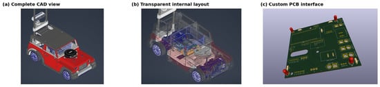
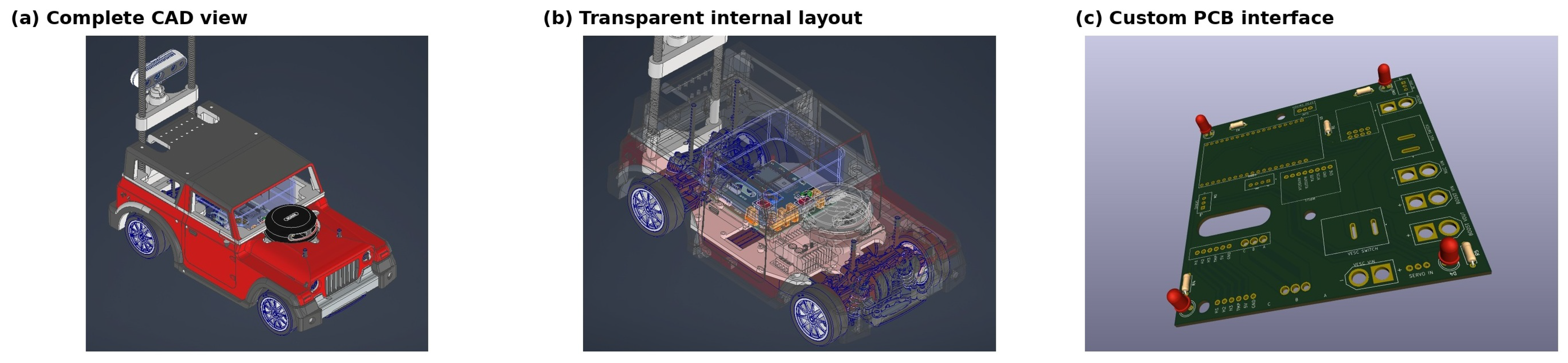
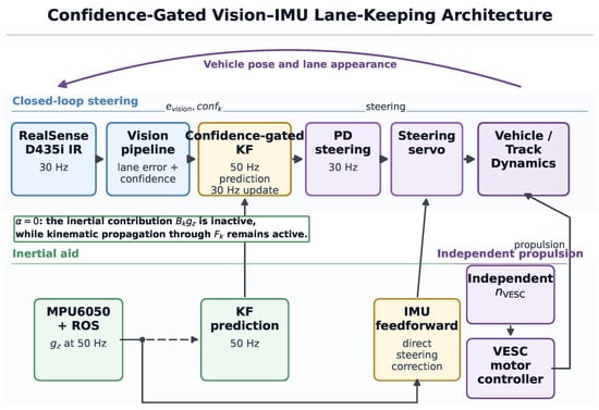
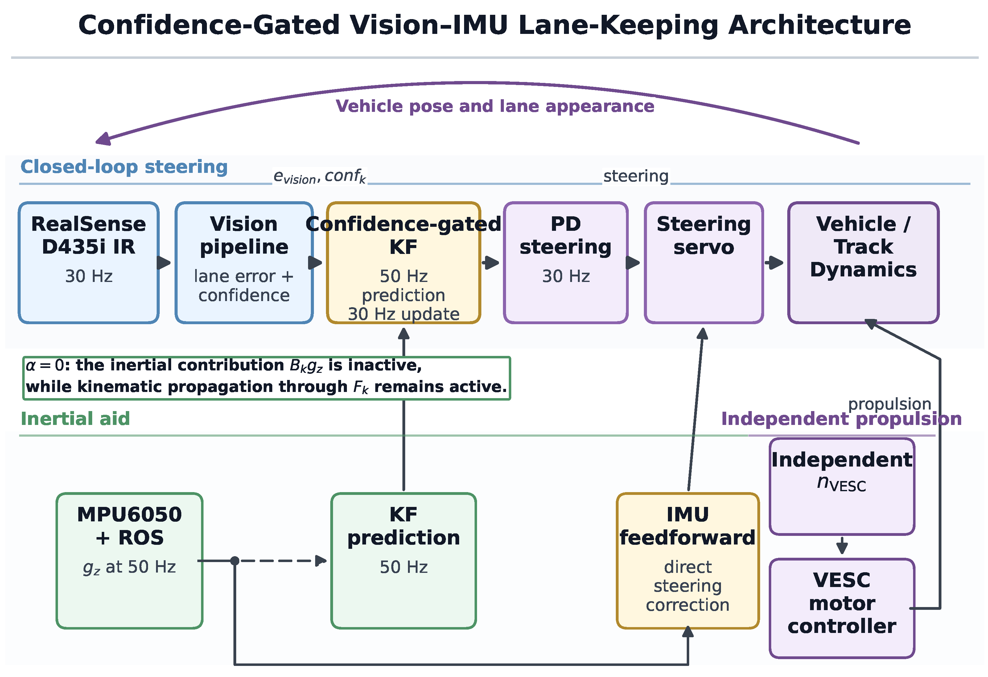
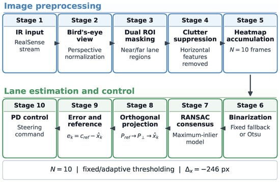
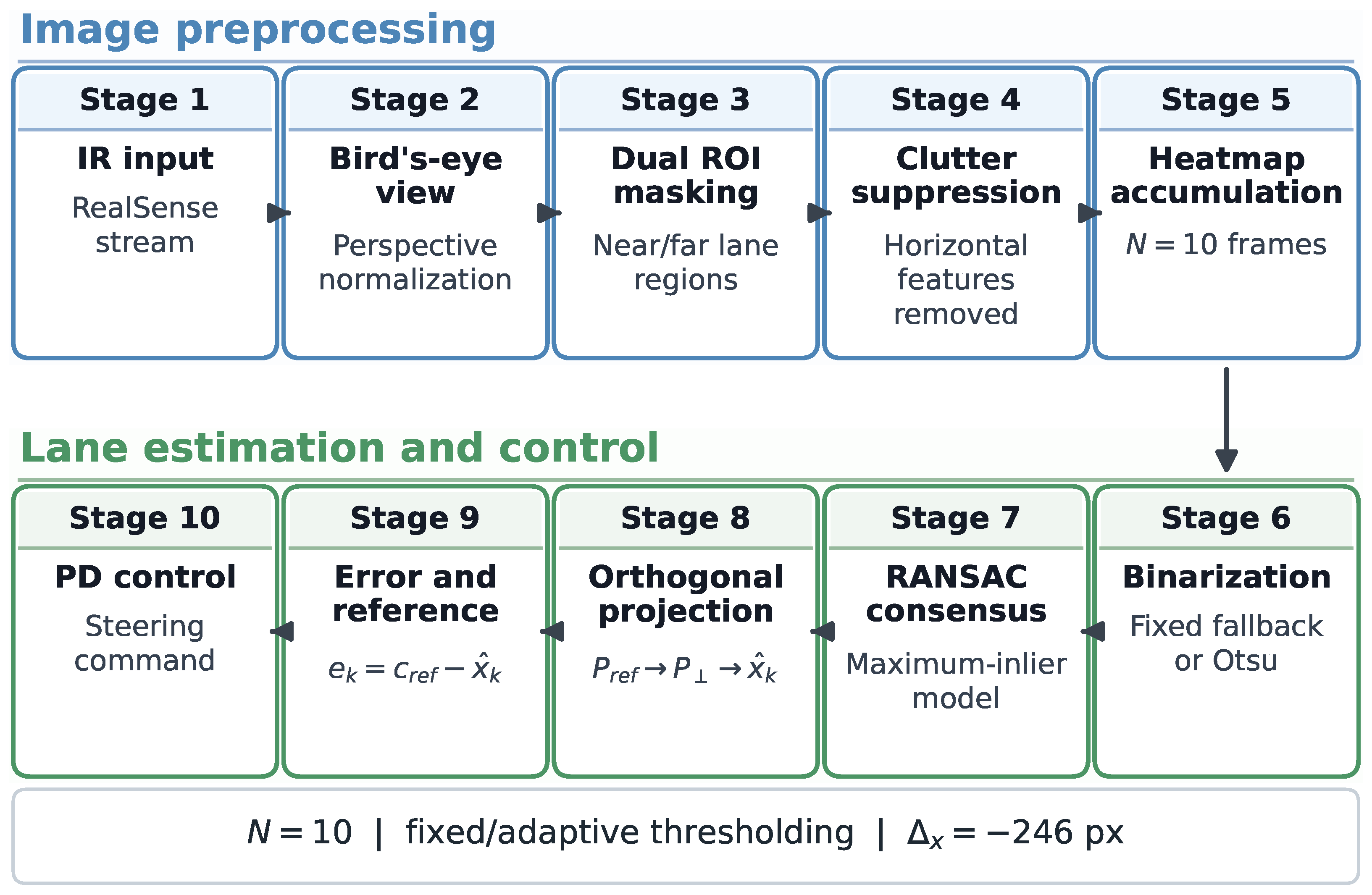
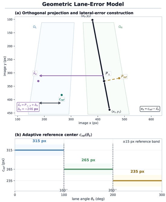
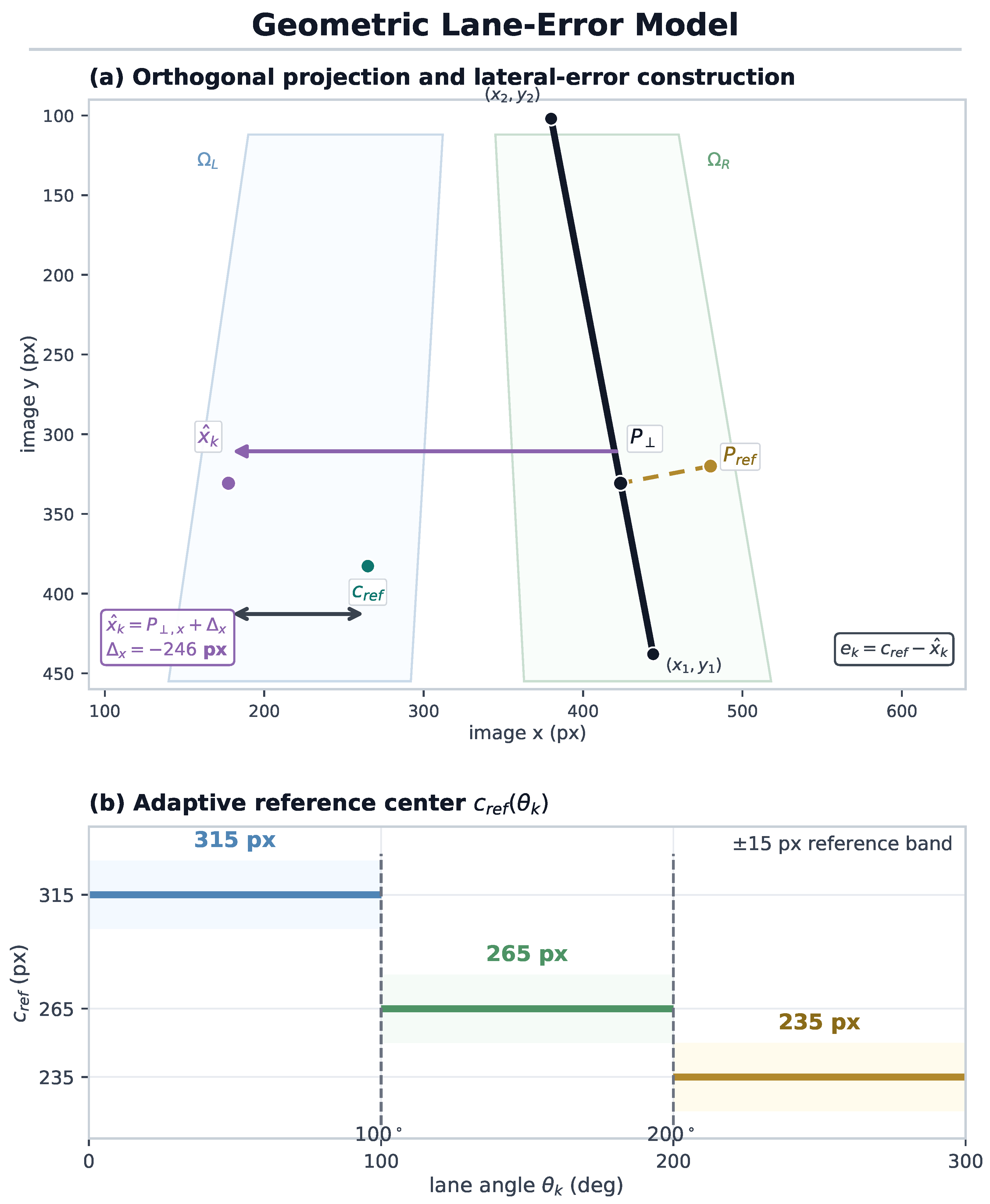
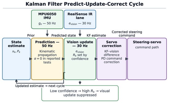
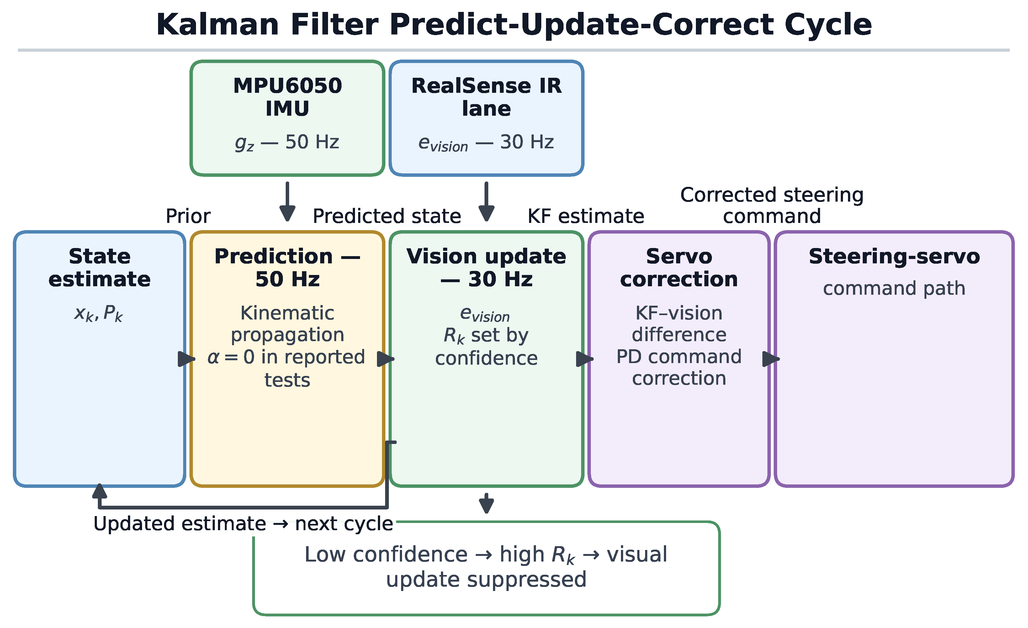
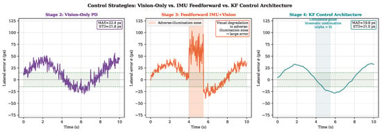
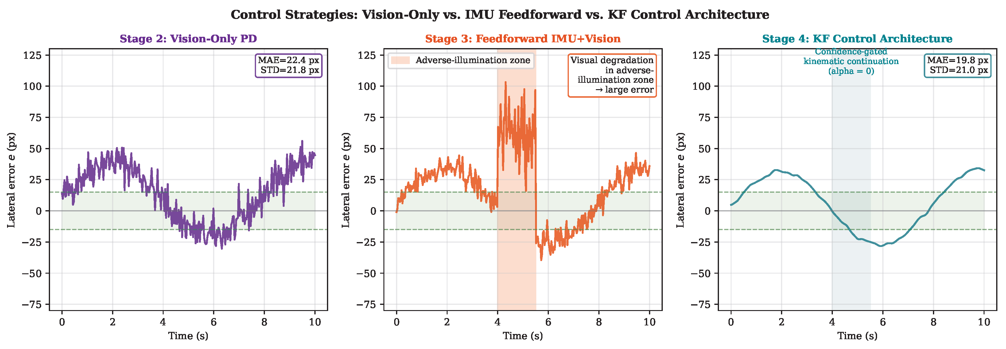
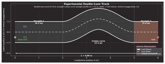
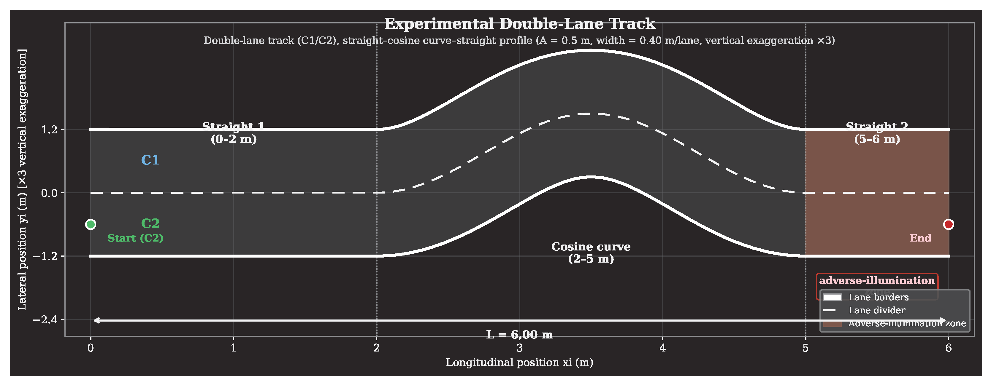
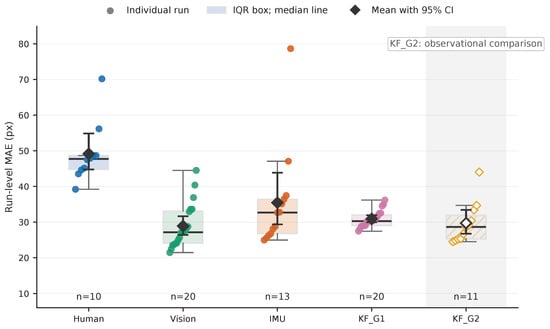
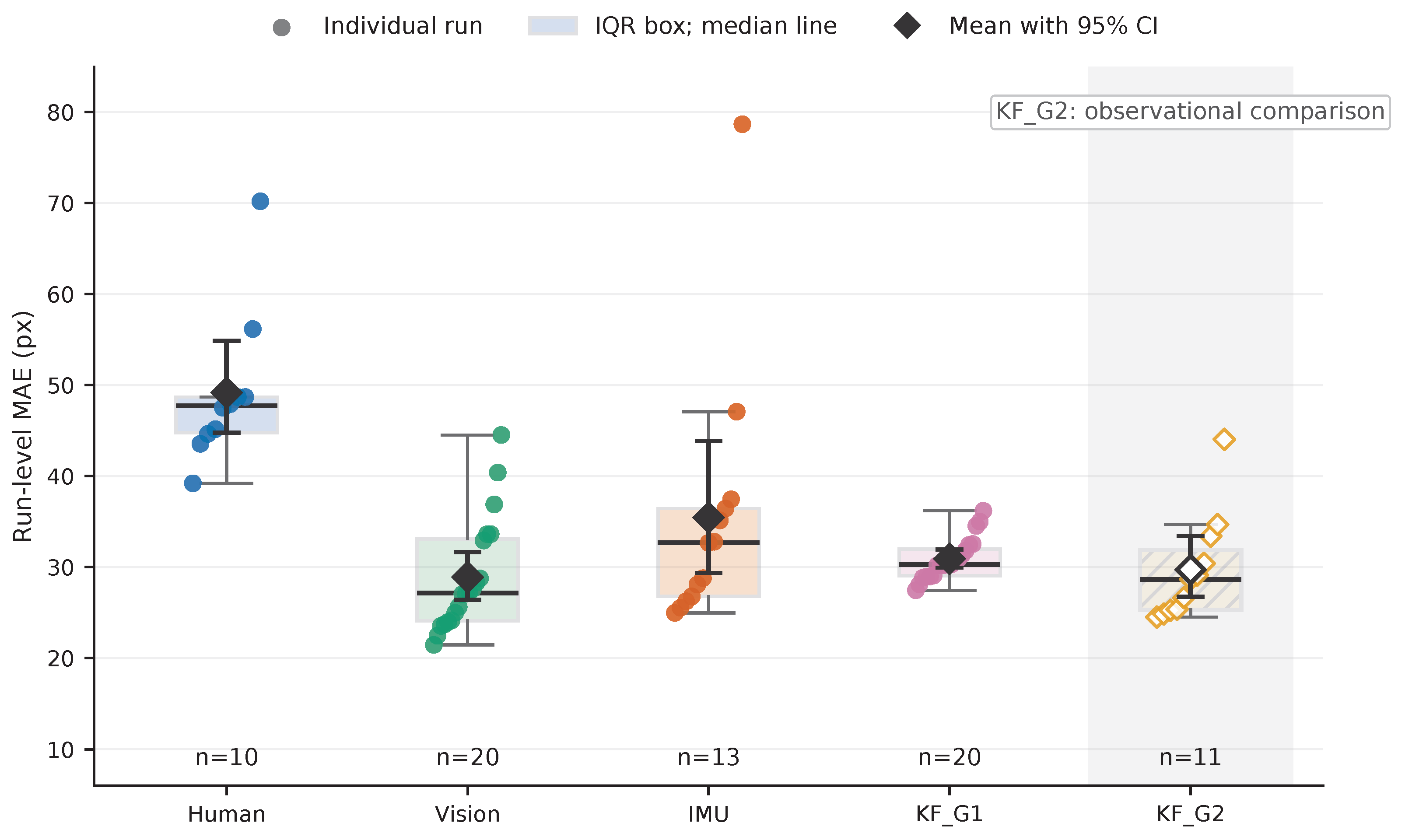
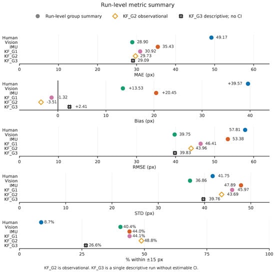
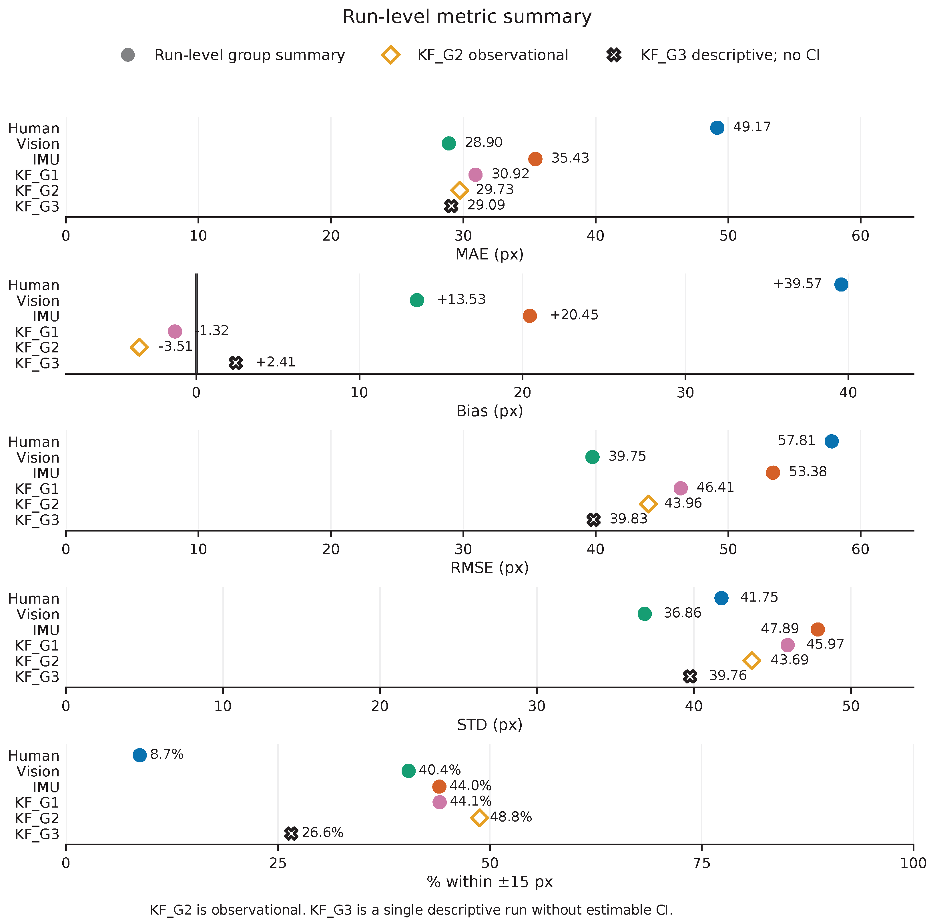
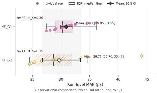
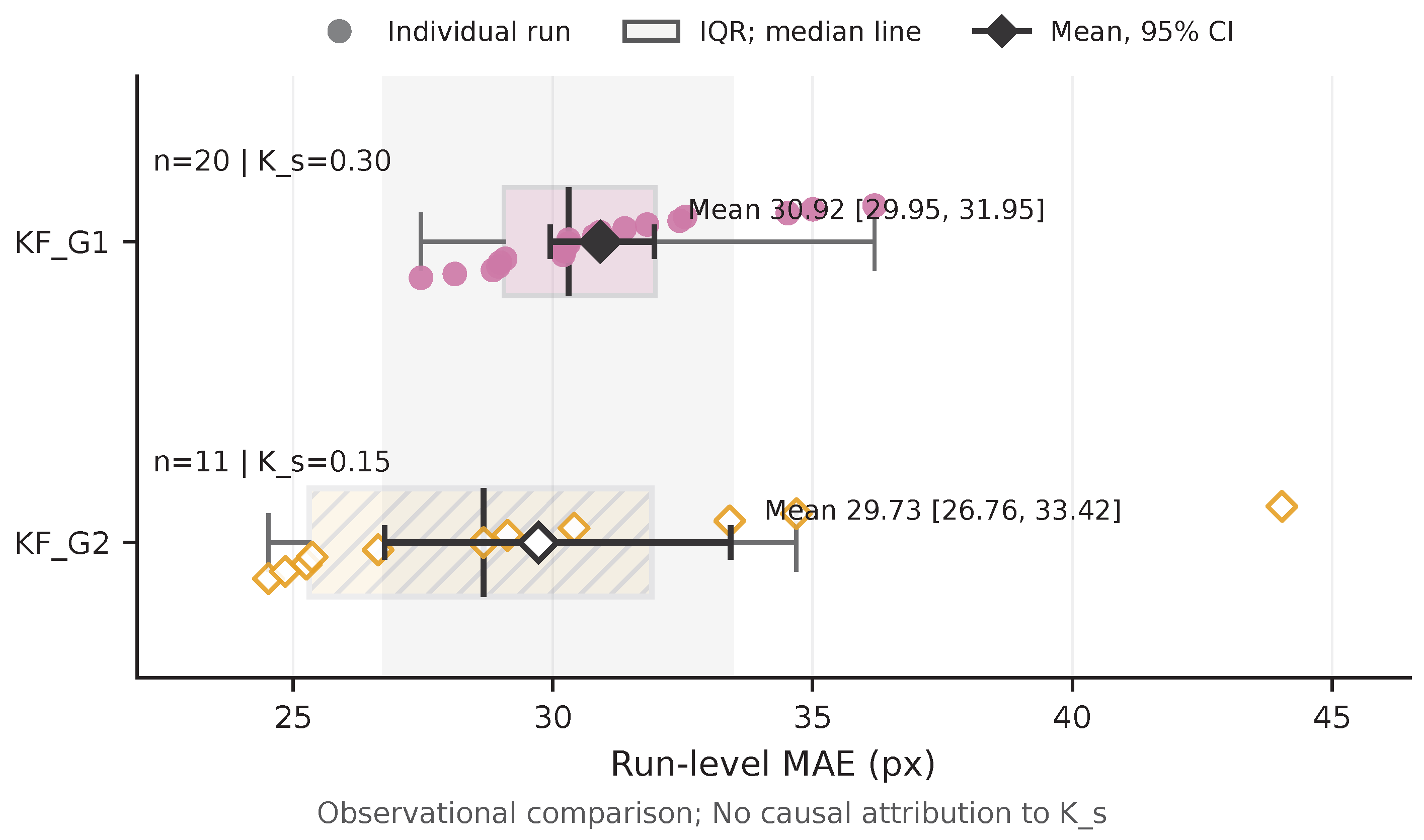
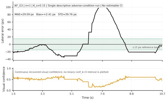
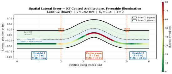
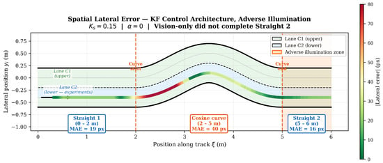
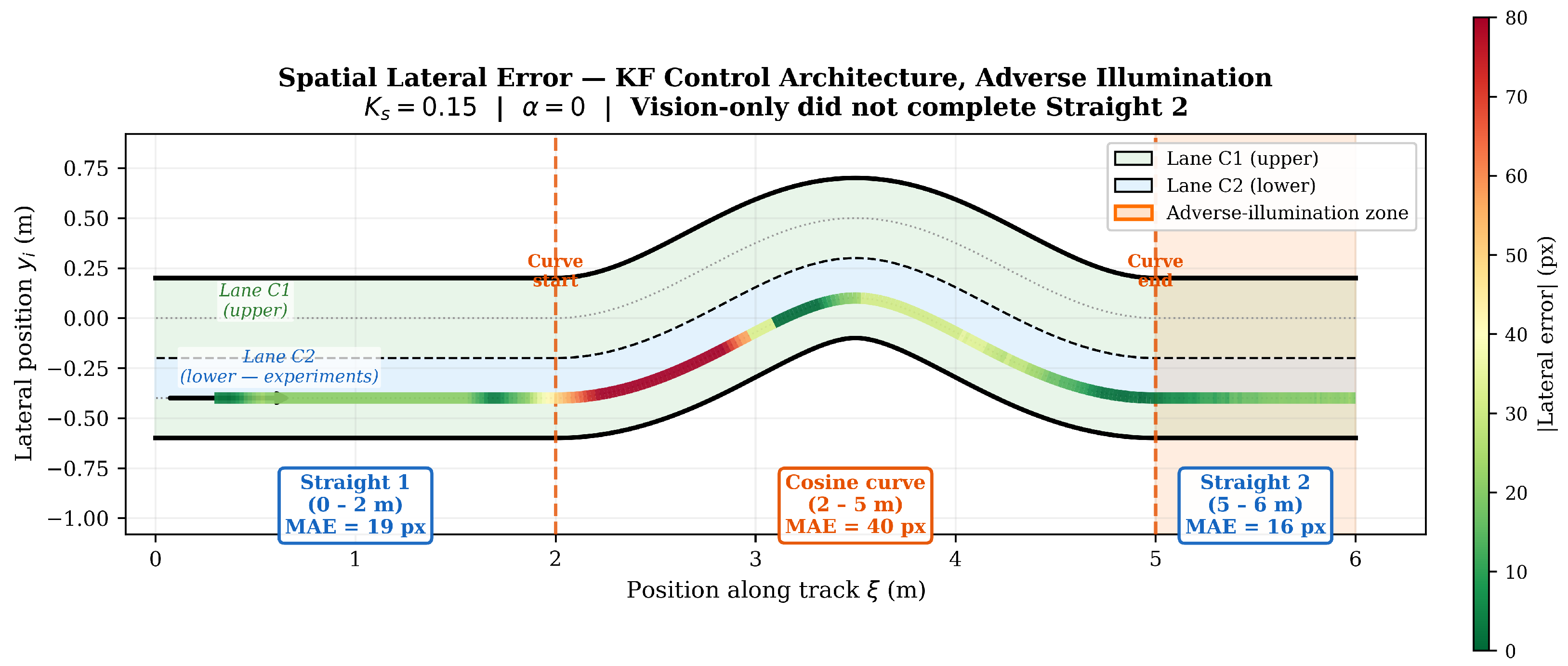
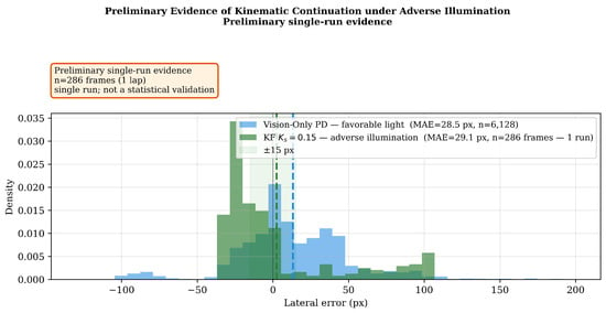
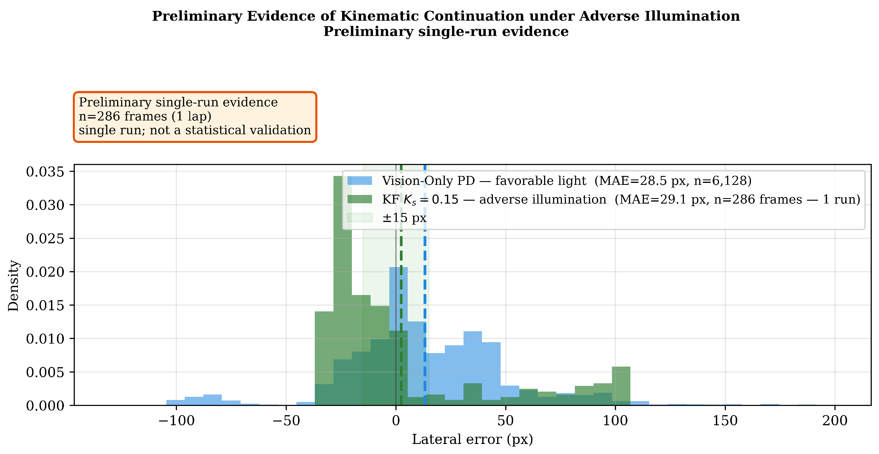
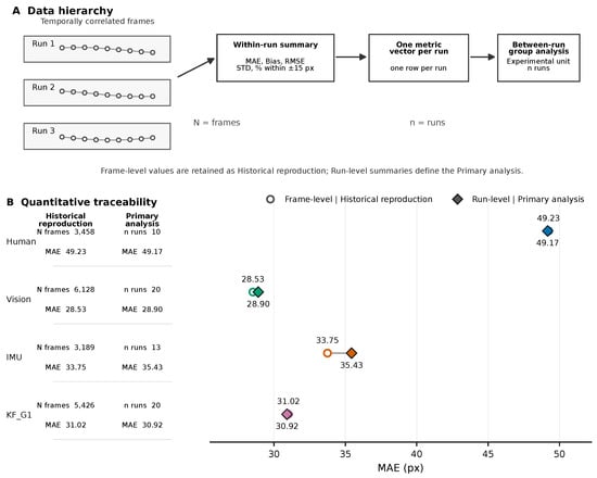
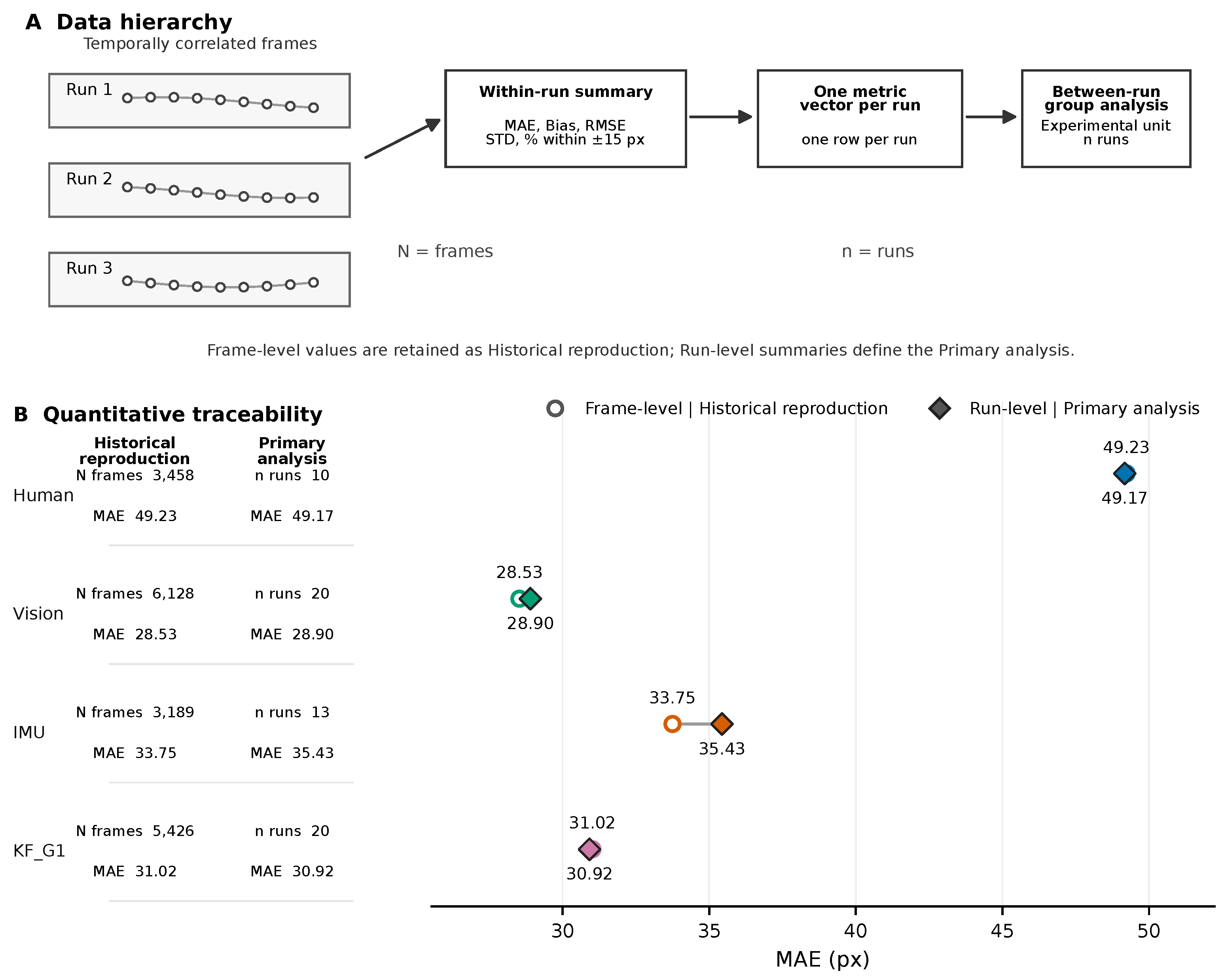

Disclaimer/Publisher’s Note: The statements, opinions and data contained in all publications are solely those of the individual author(s) and contributor(s) and not of MDPI and/or the editor(s). MDPI and/or the editor(s) disclaim responsibility for any injury to people or property resulting from any ideas, methods, instructions or products referred to in the content. |
© 2026 by the authors. Licensee MDPI, Basel, Switzerland. This article is an open access article distributed under the terms and conditions of the Creative Commons Attribution (CC BY) license.