Article

Vision-Map Fusion Multi-Object Tracking at Complex Intersections Using HD Map Priors and Nonlinear Filtering


by
Dezheng Ma
and
Lan Tang
*
School of Automobile and Transportation, Xihua University, Chengdu 610039, China
*
Author to whom correspondence should be addressed.
Automation 2026, 7(4), 130; https://doi.org/10.3390/automation7040130
Submission received: 25 June 2026 / Revised: 12 August 2026 / Accepted: 14 August 2026 / Published: 16 August 2026
(This article belongs to the Section Smart Transportation and Autonomous Vehicles)

Highlights

What are the main findings?
  • A map-aided dual-box perception frontend assigns straight-driving and turning re-gions to HBB and OBB branches, respectively, and converts both outputs into a com-mon observation format.
  • A central-difference state estimator is combined with HD-map lane feasibility con-straints to reduce physically implausible trajectory drift.
What are the implications of the main findings?
  • On the evaluated public sequences, the complete configuration achieved a favorable MOTA/IDF1/IDS balance while retaining real-time throughput on a desktop GPU workstation.
  • A single-intersection Vehicle-in-the-Loop case study using RTK reference data yield-ed an overall MAE of 0.180 m; this result is descriptive rather than a multi-site accu-racy guarantee.

Abstract

Accurate multi-object tracking and metric localization support traffic monitoring and cooperative intelligent transportation at complex intersections. This study presents a fixed-camera vision-map fusion framework that addresses two practical difficulties: axis-aligned boxes poorly represent turning vehicles, and unconstrained image-plane tracking can produce physically implausible trajectories. A map-aided frontend first generates candidate detections using improved You Only Look Once version 8 nano (YOLOv8n) horizontal bounding box (HBB) branch and an improved YOLOv8 oriented bounding box (OBB) branch. A high-definition (HD) map selector then retains the candidate geometry consistent with the straight-driving or turning region and converts it into a unified detection record. The selected reference point is projected to the ground plane through an offline-estimated homography, whereas the appearance feature bypasses the homography and is passed directly to the association stage. The tracking backend uses a 12-dimensional joint image/metric state, symmetric central-difference evaluations of the process and measurement functions, appearance-motion association, and a feasible-road projection derived from HD-map lane polygons. On the evaluated public sequences, the complete configuration achieved a multiple object tracking accuracy (MOTA) of 74.5%, an identification F1 score (IDF1) of 82.6%, 614 identity switches, and a throughput of 26.8 frames per second (FPS) on an RTX 4090 workstation. In a descriptive Vehicle-in-the-Loop case study involving one instrumented vehicle at one intersection, the overall localization mean absolute error (MAE) was 0.180 m, compared with 0.208 m for the baseline end-to-end configuration. These results indicate the feasibility of combining branch-specific vehicle geometry with map-constrained tracking; controlled same-detector comparisons, repeated multi-vehicle trials, and embedded-device latency and power profiling remain necessary for broader claims.

1. Introduction

Intersections are critical nodes in urban traffic networks, where monitoring accuracy affects signal control, safety analysis, and cooperative intelligent transportation [1,2]. Their visual complexity arises from intersecting traffic streams, heterogeneous road users, frequent occlusion, illumination changes, and abrupt changes in vehicle heading. A roadside tracking system must therefore preserve target identity while also producing locations that remain meaningful in the road coordinate system.
Recent vision-based road-transport studies have adopted one-stage You Only Look Once (YOLO) detectors because they offer a useful accuracy-throughput compromise [3,4]. However, horizontal bounding boxes (HBBs) include increasing background area when a vehicle turns, whereas applying oriented bounding boxes (OBBs) over an entire intersection can increase computation. This motivates a spatially selective design in which the map determines where HBB or OBB geometry is used, rather than treating one representation as optimal for every part of the scene.
Tracking-by-detection methods such as Simple Online and Realtime Tracking (SORT), DeepSORT, and StrongSORT combine motion prediction with data association [5,6,7]. Recent work in Automation has also emphasized continuity under missed detections and posture-aware multi-target tracking [8,9]. At intersections, constant-velocity image-plane prediction is challenged by curved motion, acceleration, scale changes, and long occlusion. Moreover, a visually smooth track can still cross a curb or opposing lane because image-plane estimators do not encode the drivable topology.
To address these linked issues, this paper develops a fixed-camera vision-map fusion framework. The frontend generates HBB and OBB candidate detections and then uses the high-definition (HD) map regions, together with the detection reference point or predicted track point, to select the appropriate candidate representation. The backend converts the selected candidate into a unified observation, projects only its reference point into the metric plane, and passes the appearance feature directly to the association stage. It then performs central-difference state estimation and appearance–motion association and projects the posterior position to the nearest drivable-map location only when it lies outside the feasible road set. Unlike camera–radar fusion [10], the operational inputs remain a monocular roadside video stream and a pre-registered static map; the real-time kinematic (RTK) receiver is used only as an evaluation reference.
The contributions are summarized as follows:
  • A unified vision-map tracking formulation is introduced in which image-plane and metric-plane variables are maintained in one state, and HD-map lane polygons provide an explicit feasibility correction for off-road predictions.
  • A map-aided dual-box frontend combines an HBB branch enhanced with a cross-stage partial bottleneck with two convolutions and squeeze-and-excitation (C2fSE), dense atrous spatial pyramid pooling (DenseASPP), and Wise-IoU version 3 (WIoU v3) training loss with an OBB branch enhanced with spatial pyramid pooling-fast (SPPF), large separable kernel attention (LSKA), and DySample. Both branches first generate candidate detections. An HD-map selector subsequently retains the appropriate HBB or OBB representation and constructs a common detection record without reinitializing the tracker identity.
  • Public-dataset detection and tracking results are complemented by a single-site RTK-referenced case study. The study reports the observed metric error and explicitly distinguishes this descriptive validation from multi-site or embedded-deployment verification.

2. Related Work

2.1. Limitations of HBB-Based Detection Algorithms

One-stage detectors, particularly YOLO variants, are widely used for road-object perception because of their speed and compact model families [3,4]. End-to-end transformer detectors provide another real-time design direction [11]. Recent studies in Sensors and Electronics have examined YOLO-based roadside vehicle detection, camera–radar fusion, and deployment on constrained edge devices [4,10]. These studies also show that workstation throughput cannot be transferred directly to embedded hardware without device-specific latency, memory, and power measurements [4]. For the straight-driving branch, the present work retains HBB geometry and targets occlusion and scale variation through channel recalibration, dense atrous context, and dynamic box-regression focusing.
OBB detection represents vehicle orientation more directly and is useful for turning or diagonally viewed vehicles. Region-of-interest (RoI) Transformer is an early representative approach for oriented detection [12], while Rope3D provides roadside orientation and 3D annotations for traffic perception [13]. DenseASPP aggregates context at several dilation rates [14], and DySample learns sampling offsets for lightweight upsampling [15]. Rather than treating either box representation as universally optimal, the proposed frontend generates HBB and OBB candidates and uses map-defined straight-driving and turning regions to select the appropriate candidate geometry before tracking.

2.2. Vision-Based Multi-Object Tracking and Localization

Tracking-by-detection associates frame-wise observations with predicted tracks. ByteTrack and ByteTrackV2 preserve low-confidence detections to improve association continuity [16,17], whereas DeepSORT and StrongSORT add appearance information and stronger association or motion components [5,6]. Recent approaches have also addressed missed detections or posture-specific tracking in other application domains [8,9]. The present study focuses on fixed-camera vehicle motion at intersections and evaluates a central-difference state estimator derived from symmetric evaluations of nonlinear process and measurement functions [18].
Metric localization from a fixed monocular camera requires an explicit scene model. For an approximately planar road surface, a homography can map image reference points to a ground-plane coordinate system under the standard projective-geometry model [19], with robust estimation based on feature or control-point correspondences [20,21]. MapTR and MapTRv2 instead learn online vectorized HD-map representations [22,23], while BEVFusion and BEVFormer construct bird’s-eye-view (BEV) representations from multiple sensors or multiple camera views [24,25]. The present method uses a pre-registered static map as prior information rather than a second live sensor. Camera-radar or camera–light detection and ranging (LiDAR) systems provide complementary measurements [10] but require additional sensing, synchronization, and calibration. The fixed-camera configuration reduces online sensor requirements but remains sensitive to camera motion, non-planar road geometry, adverse weather, and calibration drift.

3. Proposed Methodology

3.1. Problem Formulation and System Overview

This section defines the proposed fixed-camera multi-object tracking and localization framework. The online source is a calibrated roadside image sequence. The static map contains lane polygons, centerlines, and map-defined regions of interest. The homography H map between image and local ground coordinates is estimated offline and is not recomputed for every frame.
The method is organized into five layers. Layer 1 acquires roadside video, map geometry, and offline camera-map control points. Layer 2 performs map-aided dual-box perception. Layer 3 converts the selected detection reference point from image coordinates to a common six-dimensional joint metric–image measurement vector. Layer 4 predicts, associates, updates, and, when required, projects the track onto the feasible road set. Layer 5 outputs track identities, image and metric trajectories, and evaluation metrics.
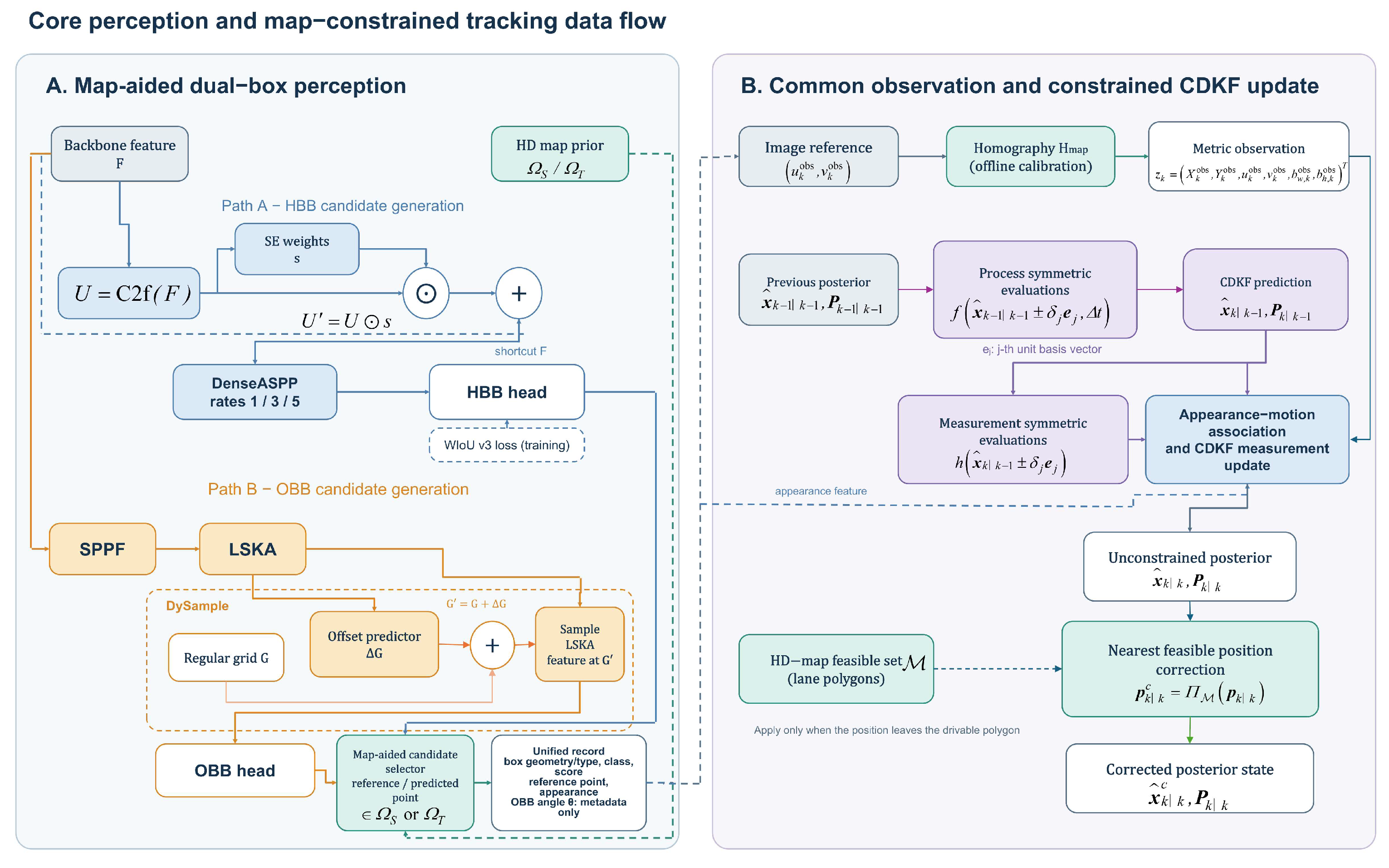
Figure 1 follows these five layers explicitly. The HBB and OBB branches first generate candidate detections. The map-aided selector evaluates the reference point of an unmatched detection or the predicted metric point of an active track against the straight-driving region Ω S and turning region Ω T , and then retains the appropriate candidate representation. The selected candidate is converted into a unified record containing the box geometry and type, class, score, reference point, appearance feature, and, when available, the OBB angle θ as detection metadata. Only the reference point is projected through the homography H map to form the six-dimensional joint metric–image measurement vector z k = X k obs , Y k obs , u k obs , v k obs , b w , k obs , b h , k obs T . The appearance feature does not belong to z k and therefore bypasses the homography and directly enters the appearance–motion association stage. The previous posterior state enters central difference Kalman filter (CDKF) prediction, while the predicted state and covariance, current six-dimensional joint metric–image measurement vector, and appearance feature jointly support association and measurement update. The resulting posterior position is corrected only when it leaves the HD-map feasible set.
Abbreviations: HD, high-definition; HBB, horizontal bounding box; OBB, oriented bounding box; C2f, cross-stage partial bottleneck with two convolutions; C2fSE, C2f with squeeze-and-excitation; DenseASPP, dense atrous spatial pyramid pooling; WIoU v3, Wise-IoU version 3; SPPF, spatial pyramid pooling-fast; LSKA, large separable kernel attention; CDKF, central difference Kalman filter; ID, identity; 2D, two-dimensional; MOTA, multiple object tracking accuracy; IDF1, identification F1 score; IDS, identity switches; FPS, frames per second; RTK, real-time kinematic.

3.2. Spatial-Decoupled Dual-Box Perception Frontend

The intersection ROI is partitioned into a straight-driving set Ω S and a turning set Ω T using HD-map lane polygons. Both detector branches first produce candidate detections. The selector then evaluates the predicted metric reference point of each active track and the reference point of each unmatched detection. Candidates associated with Ω S retain HBB geometry, whereas candidates associated with Ω T retain OBB geometry. A branch label is metadata attached to an observation rather than a tracker identity, and both representations share the same downstream observation schema and tracker pool.
For detections assigned to Ω S , the YOLOv8n HBB branch is used. Its three modifications have distinct roles.
  • C2fSE channel recalibration: A squeeze-and-excitation (SE) [26] is embedded in the C2f path. The C2f output follows two paths: one produces channel weights and the other supplies the unweighted transformed feature to element-wise multiplication. The reweighted feature is then added to the unchanged shortcut feature. Figure 2 shows both inputs to the multiplication and residual-addition nodes explicitly.
  • DenseASPP context aggregation: Densely connected atrous convolutions with dilation rates 1, 3, and 5 aggregate multiple receptive fields without an additional reduction in feature-map resolution [14]. This module targets the scale variation between small distant vehicles and large near-field vehicles.
  • WIoU v3 regression loss: The non-monotonic focusing mechanism adjusts the contribution of anchors according to their outlier degree [27]. Its purpose is to reduce the dominance of very low-quality samples during box regression; it does not guarantee that every intermediate ablation will improve every metric.
For detections assigned to Ω T , the YOLOv8-OBB branch returns an oriented box parameterized by center coordinates, width, height, and heading angle. At the Ω S / Ω T boundary, the branch label may change between frames, but the metric reference point, appearance descriptor, and predicted track state are passed to the same association stage. The track identifier and covariance are not reset. If both ROIs overlap, candidate detections are transformed to the common space and the candidate with the lower gated association cost is retained, which reduces duplicate updates and identity fragmentation.
  • SPPF-LSKA attention: LSKA [28] is embedded after spatial-pyramid pooling to capture long-range spatial dependencies using separable large-kernel operations. This is intended to retain elongated vehicle structure during turns without applying a dense large 2D kernel.
  • DySample upsampling: The LSKA feature is supplied to a lightweight offset predictor to estimate the sampling offset Δ G . The regular grid G does not enter the offset predictor; instead, G and Δ G are combined only at the addition node to form G = G + Δ G . The LSKA feature is then sampled at G , and the resulting feature is decoded into OBB confidence, category, center, size, and angle [15].
Figure 2 links the perception frontend to the tracking backend at the data-flow level. Panel A shows that the C2f output U supplies both the SE-weight generation path and the feature-reweighting path. In the DySample block, the LSKA feature predicts Δ G , the regular grid G bypasses the offset predictor, and G and Δ G are added to form G before feature sampling. Panel B separates process prediction from measurement processing. The previous posterior generates the predicted state and covariance, which are supplied both to the measurement-function evaluations and directly to appearance–motion association for motion gating. The current six-dimensional joint metric–image measurement vector and appearance feature enter the association and measurement-update stage through separate paths; the appearance feature is not included in z k and is not transformed by the homography. The implemented map operation remains a direct nearest-feasible projection rather than an iterative quadratic-programming loop.

3.3. Map-Constrained CDKF Tracking and Localization Backend

The backend extends a DeepSORT-style tracking-by-detection pipeline with a joint image/metric state and a map-feasibility operation. The estimator is referred to as a Central Difference Kalman Filter (CDKF) because local process and measurement sensitivities are obtained from symmetric function evaluations rather than analytic Jacobians [18].
Let the observed image reference point and its corresponding local ground-plane point be related through the standard planar projective model [19], as expressed in Equation (1). The image-to-ground homography H map is estimated offline from paired camera-map control points using scale-invariant feature transform (SIFT) descriptors [21] and random sample consensus (RANSAC) [20]. Equation (2) gives the dehomogenized metric coordinates. The HBB bottom center and the OBB ground-contact reference point are both converted by this mapping. Because the planar model is a 2D-to-2D projective mapping, the output is a metric ground-plane observation rather than a full 3D reconstruction.
λ k X k obs Y k obs 1 = H map u k obs v k obs 1 , H map = h i j map 3 × 3
X k obs = h 11 map u k obs + h 12 map v k obs + h 13 map h 31 map u k obs + h 32 map v k obs + h 33 map , Y k obs = h 21 map u k obs + h 22 map v k obs + h 23 map h 31 map u k obs + h 32 map v k obs + h 33 map .
In Equations (1) and (2), k denotes the time-step index; ( u k obs , v k obs ) denotes the observed image-plane reference point in pixels; and ( X k obs , Y k obs ) denotes the corresponding observed ground-plane position in meters. The non-zero scalar λ k is the homogeneous scale factor. The matrix H map 3 × 3 is the image-to-ground homography, and h i j map ,   i , j { 1 , 2 , 3 } , denotes its element in the i-th row and j-th column. The superscript obs identifies a measured quantity, and the superscript T denotes matrix transpose.
At time step k , the 12-dimensional state of each active track contains metric position, metric velocity and acceleration, image-plane position and velocity, and bounding-box dimensions. The six-dimensional measurement contains the observed metric position, image-plane reference point, and bounding-box dimensions, as defined in Equation (3).
x k = X k , Y k , V X , k , V Y , k , a X , k , a Y , k , u k , v k , V u , k , V v , k , b w , k , b h , k T , z k = X k obs , Y k obs , u k obs , v k obs , b w , k obs , b h , k obs T .
In Equation (3), x k 12 is the state vector of an active track at time step k , and z k 6 is the corresponding measurement vector. The variables X k and Y k are the metric ground-plane coordinates in meters; V X , k and V Y , k are the metric velocities in meters per second; and a X , k and a Y , k are the metric accelerations in meters per second squared. The variables u k and v k are the image-plane coordinates in pixels, whereas V u , k and V v , k are their image-plane velocities in pixels per second. The variables b w , k and b h , k denote the bounding-box width and height in pixels. The prefix b distinguishes the bounding-box dimensions from the process and measurement functions.
Equation (4) defines the stochastic process and measurement models. The function f propagates the metric components with a constant-acceleration model and the image components with a constant-velocity model. The process noise has covariance Q. The function h selects or nonlinearly maps the predicted state into the six measured quantities, and the measurement noise has covariance R.
x k = f x k 1 , Δ t + q k 1 , q k 1 ~ N 0 , Q , z k = h x k + r k , r k ~ N 0 , R .
In Equation (4), f : 12 × + 12 is the state-transition function, h : 12 6 is the measurement function, and Δ t is the elapsed time between two consecutive frames in seconds. The vectors q k 1 and r k are the zero-mean process and measurement noises, respectively. Their covariance matrices are Q 12 × 12 and R 6 × 6 . The notation N ( 0 , Q ) denotes a Gaussian distribution with zero mean and covariance Q , with an analogous definition for N 0 , R .
J f : , j f x ^ k 1 | k 1 + δ j e j , Δ t f x ^ k 1 | k 1 δ j e j , Δ t 2 δ j , J h : , j h x ^ k | k 1 + δ j e j h x ^ k | k 1 δ j e j 2 δ j , j = 1 , , 12
.
In Equation (5), J f 12 × 12 and J h 6 × 12 denote the process and measurement sensitivity matrices, respectively, and ( ) : , j denotes the j-th matrix column. The vector e j 12 is the j-th unit basis vector, and δ j > 0 is the central-difference perturbation applied to the j-th state component. The estimate x ^ k 1 | k 1 is the posterior state at the previous time step, whereas x ^ k | k 1 is the current prior state. More generally, the notation k / l denotes an estimate at time k conditioned on observations available through time l . The matrices P k 1 | k 1 ,   P k | k 1 , and P k | k denote the previous posterior, current prior, and current posterior error covariances, respectively. The current observation z k is not used as an input to state prediction; it enters only the association and measurement-update stage.
Let p ^ k | k = [ X ^ k | k , Y ^ k | k ] T denote the unconstrained posterior metric position extracted from x ^ k | k , and let M denote the union of legally drivable lane polygons. The map-feasibility operation is defined in Equation (6).
p ^ k | k c = p ^ k | k , p ^ k | k M , Π M p ^ k | k arg min p M p p ^ k | k 2 , p ^ k | k M .
In Equation (6), the superscript c denotes a map-corrected quantity, Π M ( ) is the Euclidean projection onto the feasible set M , and 2 denotes the Euclidean norm. When the posterior position lies outside M , only its metric position components are replaced by the nearest feasible point; track identity, appearance history, and covariance history are retained. This deterministic geometric projection is triggered only for an off-road posterior.

4. Experiments, Results, and Discussion

4.1. Experimental Setup and Implementation Details

Experiments used the official partitions of four public datasets. The University at Albany Detection and Tracking (UA-DETRAC) benchmark [29] contains 100 traffic videos and more than 140,000 annotated frames at 960 × 540 resolution; VisDrone2019 [30] contains 6471 training, 548 validation, and 1580 test images; the Berkeley DeepDrive 100K (BDD100K) dataset [31] contains 100,000 road images; and Rope3D [13] contains approximately 50,000 roadside images with more than 1.5 million 3D annotations, converted to the OBB representation used here. The HBB and OBB configurations contain 3.19 million and 3.23 million parameters and require 8.5 and 9.1 giga floating-point operations (GFLOPs) per image, respectively. All compared detection variants were trained from scratch under the same augmentation policy, with an initial learning rate of 0.02 and momentum of 0.9. Random flipping and mosaic augmentation were used. The reported 26.8 frames per second (FPS) end-to-end result was measured on an NVIDIA RTX 4090 desktop workstation; it is not an embedded-device benchmark. The physical deployment used a Jetson AGX Orin 32 GB node for acquisition and online processing. Standardized per-stage latency, peak memory, and power measurements are not reported; therefore, embedded-device deployment efficiency is not quantified in this study and remains a subject for future evaluation [4,32].

4.2. Ablation Studies on Dual-Box Perception

Ablations start from the corresponding YOLOv8 baseline and add the modules in the order shown in Table 1 and Table 2. These are sequential configurations rather than independent single-factor tests, so an intermediate row can improve one metric while reducing another.
Table 1 shows a non-monotonic HBB trend. Adding C2fSE increases precision from 96.7% to 97.5% and recall from 96.3% to 96.7%, but mean average precision at an intersection-over-union threshold of 0.5 (mAP@0.5) changes from 98.9% to 98.7%. After DenseASPP, recall rises to 96.9% while precision and mean average precision averaged over intersection-over-union thresholds from 0.5 to 0.95 (mAP@0.5–0.95) decrease to 96.1% and 88.3%. These small reversals are consistent with a precision–recall and localization trade-off: channel reweighting and larger receptive fields alter which difficult or partially occluded boxes receive high confidence. WIoU v3 then changes the regression weighting, and the complete configuration reaches 99.1% mAP@0.5 and 89.1% mAP@0.5–0.95. The table therefore supports the final combination, not a claim that each addition monotonically improves every metric.
Table 2 exhibits the same trade-off in the OBB branch. LSKA raises precision from 82.9% to 84.0%, while recall decreases from 66.8% to 66.1% and mAP@0.5–0.95 changes from 41.7% to 40.7%. A plausible mechanism is that stronger long-range attention suppresses ambiguous positives and produces a more conservative score distribution. After DySample is added, precision, recall, mAP@0.5, and mAP@0.5–0.95 reach 85.6%, 66.8%, 75.6%, and 42.7%, respectively. Because the ablation is sequential, these results should be interpreted as evidence for the complete branch configuration rather than isolated causal effects.
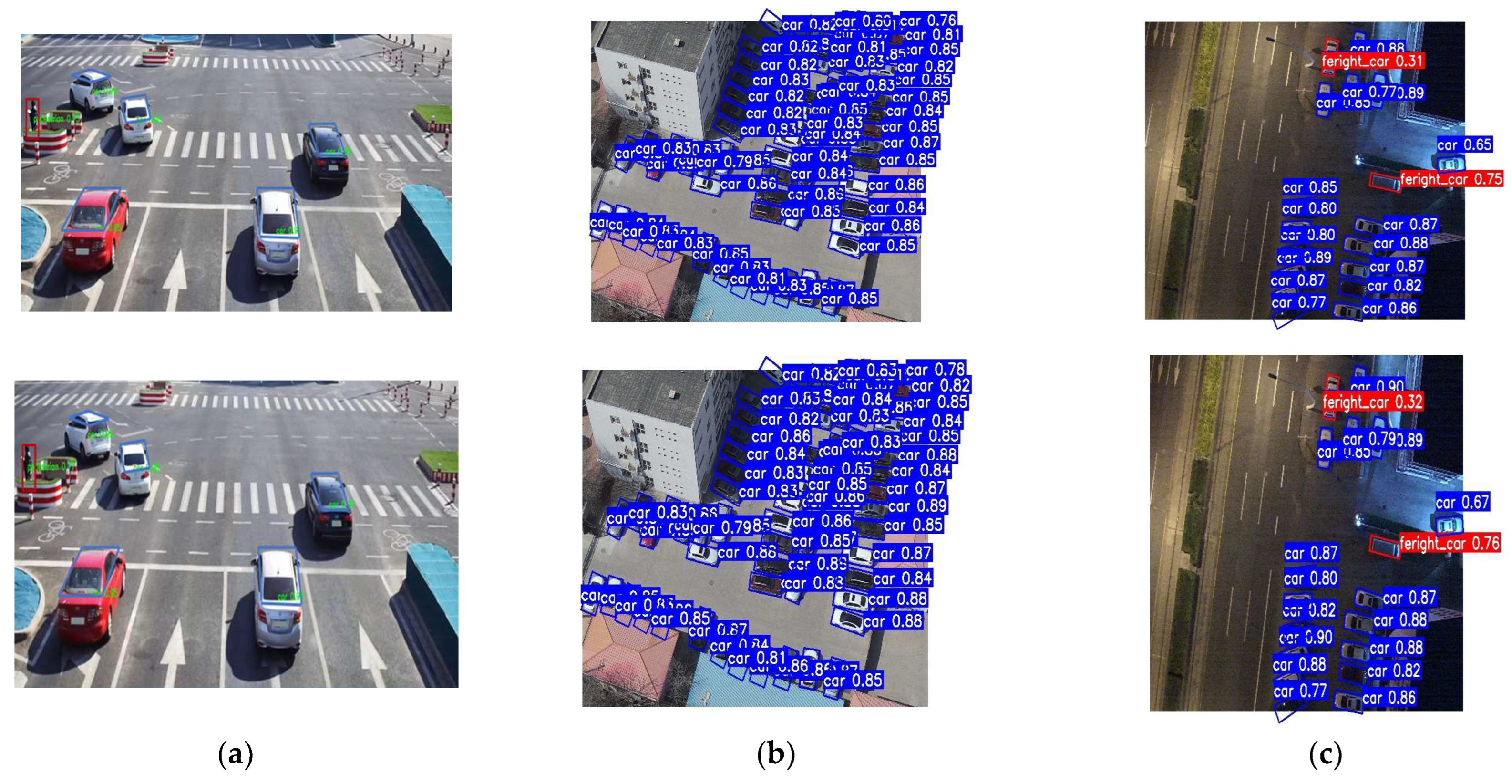
Figure 3 provides representative qualitative comparisons for turning, dense-traffic, and nighttime scenes. In the selected examples, the revised branch produces boxes that better follow inclined vehicles and retain more detections in crowded regions. These examples illustrate typical behavior but do not replace the quantitative tables; additional comparisons are provided in Appendix B.

4.3. Baseline Comparisons on Multi-Object Tracking

Table 3 compares complete tracking configurations on the evaluated intersection sequences. SORT, DeepSORT, StrongSORT, and the proposed system were not rerun with an identical frozen detection file and fully harmonized association settings. The table is therefore an end-to-end system comparison, not a controlled isolation of the CDKF and map prior.
Within this system-level comparison, the proposed configuration obtains a multiple object tracking accuracy (MOTA) of 74.5%, a multiple object tracking precision (MOTP) of 80.2%, an identification F1 score (IDF1) of 82.6%, 614 identity switches, and 26.8 FPS. StrongSORT has fewer identity switches than DeepSORT but lower throughput, while SORT is faster but less accurate. These results show a favorable accuracy–continuity–throughput balance for the full proposed pipeline. They do not establish that the difference is caused solely by the filter or map constraint; a future study should use identical detections and association thresholds and ablate CDKF and map projection separately.

4.4. Single-Intersection Validation Against an RTK Reference

The physical evaluation was conducted at one signalized urban intersection in Hangzhou, China, using one instrumented vehicle. It was designed as a Vehicle-in-the-Loop case study to check whether image-to-map trajectories were consistent with an external RTK reference. Because it covers one site and one vehicle run, the reported error is a descriptive result rather than a population estimate.
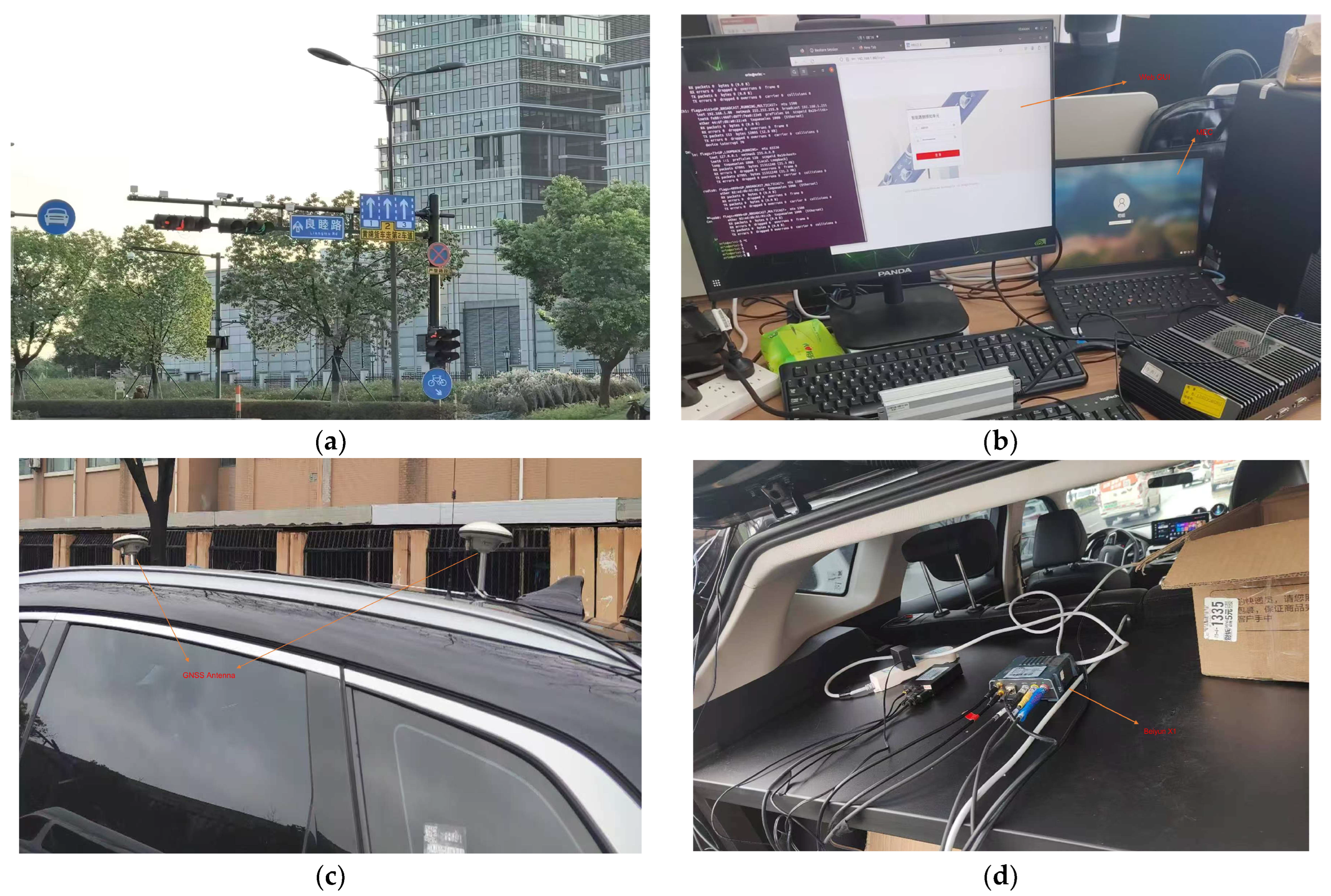
Figure 4 summarizes the instrumentation. The roadside unit used a Dahua DH-CP902-YGSL-L traffic camera with a 1.1-inch global-shutter complementary metal–oxide–semiconductor (GS-CMOS) sensor, 4096 × 2336 maximum resolution, a 25 FPS default stream (up to 50 FPS), and 100 dB wide dynamic range. The field node was an NVIDIA Jetson AGX Orin with 32 GB memory under Ubuntu 20.04 with Robot Operating System 2 (ROS 2), distinct from the RTX 4090 workstation used for the 26.8 FPS benchmark. A roof-mounted antenna and Beiyun X1 terminal recorded the reference trajectory at 10 Hz. The camera and RTK streams were recorded through ROS 2 and reviewed on the synchronized Foxglove playback timeline. The original auxiliary temporal-pairing script and the raw per-sample camera/RTK timestamp and residual files were not retained. Consequently, the acquisition-time clock specification, timestamp-offset correction, temporal-pairing rule, maximum accepted time gap, and final matched-sample count cannot be verified retrospectively. To support methodological replication without overstating the provenance of the field-trial results, a reconstructed and tested reference implementation is provided in the public release v1.0.0 at https://github.com/975032368ma-ai/vision-map-tracking-reproducibility/releases/tag/v1.0.0 (accessed on 12 August 2026). Appendix A summarizes the available configuration records, the scope of the released implementation, and the remaining limitations.
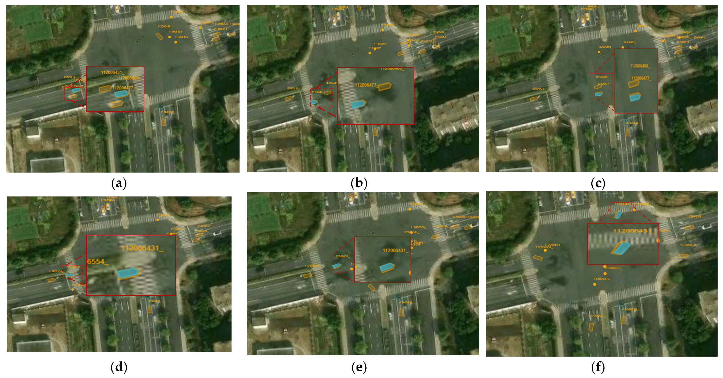
Figure 5 compares the reconstructed and RTK-referenced trajectories for representative straight and turning portions of the recorded run. In the displayed straight segments, both configurations remain close to the reference. In the displayed turning segments, the baseline trajectory shows a larger lateral departure, whereas the map-constrained trajectory remains inside the drivable polygon. This is a qualitative observation from the illustrated run and should not be generalized to untested intersections.
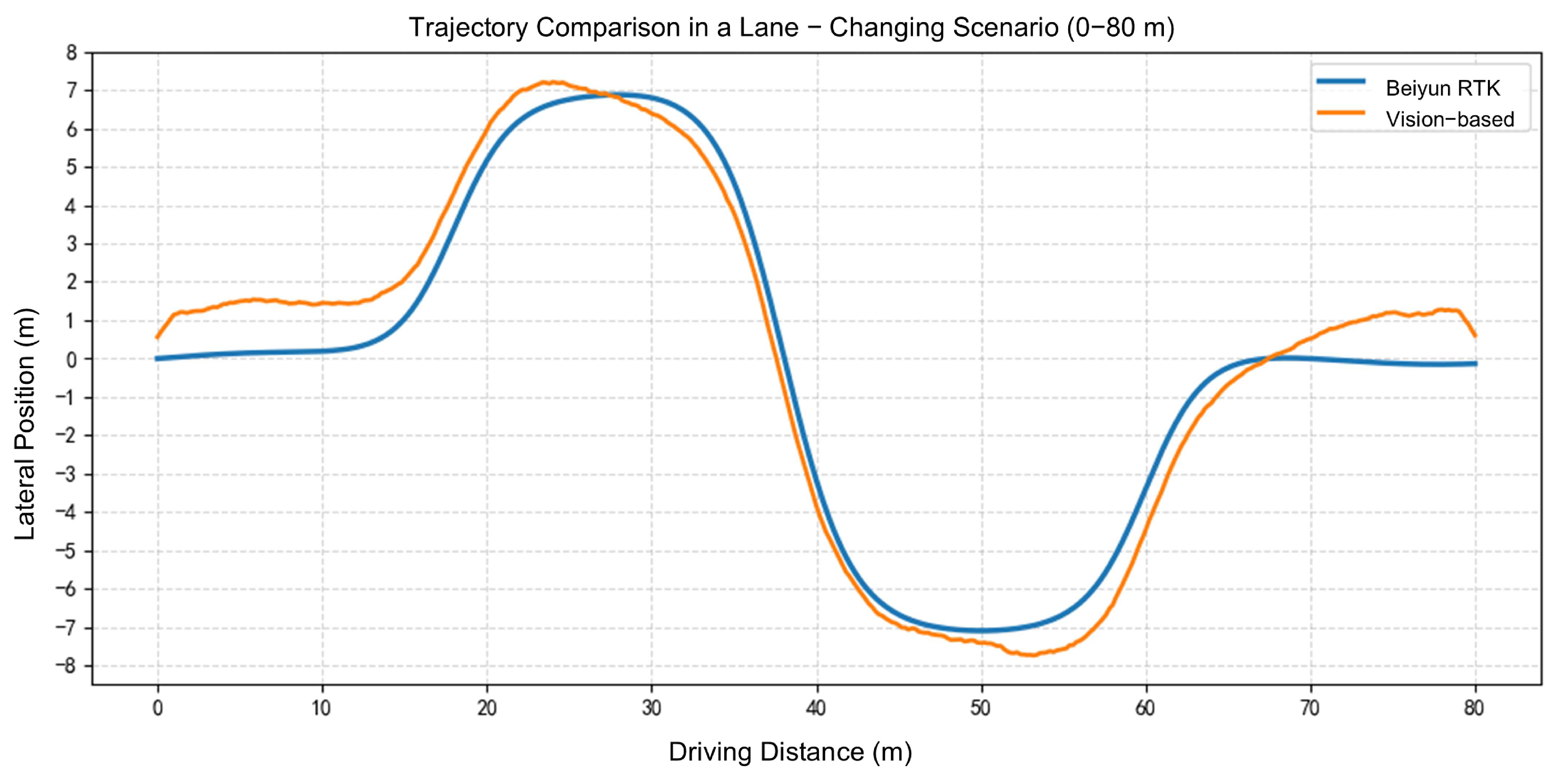
Figure 6 plots the lateral-position trajectory produced by the proposed vision-based localization pipeline together with the Beiyun RTK reference over the displayed 0–80 m trajectory segment. Table 4 separately reports aggregate mean absolute errors (MAEs) of 0.208 m for the HBB/unconstrained baseline and 0.180 m for the OBB/map-constrained configuration. Because the table changes box representation, filter, and spatial constraint together, it does not isolate the contribution of one component. Raw time-aligned residuals, the effective sample count N, and repeated trials were not reported in this study; consequently, no confidence interval or significance claim is reported.

4.5. Discussion, Computational Scope, and Limitations

The proposed approach occupies a middle ground between image-only tracking and live multi-sensor fusion. Camera-radar intersection tracking can supply complementary range or velocity measurements [10], whereas the present system uses a static HD map to regularize a monocular camera trajectory. This reduces online sensing hardware but cannot recover observations that are absent because of heavy rain, fog, glare, or complete visual occlusion.
Relative to recent automation studies, Predictive Enhancement of Detection (PrED) targets intermittent detections using prediction and similarity cues [8], while posture-aware DeepSORT improves tracking in a different occlusion-intensive domain [9]. The present contribution is distinct in its map-selected HBB/OBB geometry and explicit metric-road feasibility operation. The evidence is complementary rather than directly rankable because datasets, detectors, and target domains differ.
The reported 26.8 FPS is an aggregate workstation result. Offline homography calibration is excluded from per-frame processing, and the map correction is a direct point-in-polygon test followed, when necessary, by nearest-boundary projection rather than an iterative quadratic programming (QP) procedure. Nevertheless, reliable module-level timing was not recorded. Edge deployment studies emphasize that throughput, memory, thermal behavior, and power must be measured on the target device [4,32]; accordingly, no claim of verified Jetson real-time performance is made here.
Uncertainty is represented by the estimator covariance Q / R model, but the experiments do not calibrate predictive uncertainty. Deep Gaussian-process work illustrates how uncertainty estimation can become overconfident and motivates future calibration studies [33]. A controlled follow-up should archive frame-level residuals, report confidence intervals, harmonize detections across trackers, and measure each pipeline stage on the deployed edge node.
Appendix A summarizes the RTK update rate, ROS 2/Foxglove workflow, coordinate frame, rotation from the body frame to the vehicle frame (RBV) procedure, and the map-origin and ROI parameters used in the field trial. It also identifies the calibration and synchronization quantities that could not be quantified in this study.

5. Conclusions

This study presented a fixed-camera vision-map fusion framework for vehicle detection, tracking, and metric localization at complex intersections. The method combines map-selected HBB/OBB perception, homographic image-to-ground projection, a central-difference joint-state estimator, appearance-motion association, and a nearest-feasible-road correction.
The final HBB and OBB configurations improved the selected detection metrics relative to their corresponding baselines, although intermediate ablations were non-monotonic. In the reported end-to-end tracking comparison, the proposed system achieved MOTA of 74.5%, IDF1 of 82.6%, 614 identity switches, and 26.8 FPS on an RTX 4090 workstation. Because the baseline trackers did not share fully harmonized detections and settings, these differences cannot be attributed solely to CDKF or map constraints.
In the single-vehicle, single-intersection RTK case study, the observed localization MAE was 0.180 m for the proposed configuration and 0.208 m for the baseline configuration. This comparison supports feasibility in the recorded case but does not demonstrate universal sub-meter accuracy, statistical superiority, or robustness across sites.
The main limitations are the single-site physical evaluation, absence of repeated multi-vehicle trials and confidence intervals, lack of a fixed-detection filter ablation, and absence of per-stage latency, memory, and power measurements on the Jetson device. The fixed-camera planar homography also assumes a stable camera and locally planar road surface.
Future work will collect synchronized per-frame residuals over multiple intersections and vehicles, report uncertainty intervals, and profile detection, projection, association, state estimation, and map correction separately on embedded hardware. Radar or LiDAR can be introduced as a true complementary sensing modality for adverse weather and long occlusion [10], while predictive uncertainty models such as deep Gaussian processes may inform adaptive process and measurement covariance design [33].

Author Contributions

Conceptualization, D.M. and L.T.; methodology, D.M.; software, D.M.; validation, D.M.; formal analysis, D.M.; investigation, D.M.; resources, L.T.; data curation, D.M.; writing—original draft preparation, D.M.; writing—review and editing, D.M. and L.T.; visualization, D.M.; supervision, L.T.; project administration, L.T. All authors have read and agreed to the published version of the manuscript.

Funding

This research received no external funding.

Institutional Review Board Statement

Not applicable.

Informed Consent Statement

Not applicable.

Data Availability Statement

The public datasets used in this study are available from their respective official providers, as cited in the manuscript. Reproducibility materials, including dataset configuration templates, documentation, deterministic tests, synthetic examples, and a reconstructed reference implementation of RTK–vision temporal pairing, are publicly available in release v1.0.0 at https://github.com/975032368ma-ai/vision-map-tracking-reproducibility/releases/tag/v1.0.0 (accessed on 12 August 2026). The original auxiliary temporal-pairing script, raw per-sample camera and RTK timestamps, per-sample residual files, measured lever-arm offsets, paired map-side control points, and numerical homography from the reported field trial were not retained and therefore cannot be shared.

Acknowledgments

During the preparation of this manuscript, the authors used Grammarly (web application, accessed on 5 August 2026) and OpenAI Codex (GPT-5, accessed on 5 August 2026) solely for the purposes of English language editing and improving readability. The authors have reviewed and edited the output and take full responsibility for the content of this publication.

Conflicts of Interest

The authors declare no conflicts of interest.

Abbreviations

The following abbreviations are used in this manuscript:
BEVBird’s-Eye-View
BDD100KBerkeley DeepDrive 100K
C2fCross-Stage Partial Bottleneck with Two Convolutions
C2fSEC2f with Squeeze-and-Excitation
CARAFEContent-Aware ReAssembly of FEatures
CBAMConvolutional Block Attention Module
CDKFCentral Difference Kalman Filter
DenseASPPDense Atrous Spatial Pyramid Pooling
ECAEfficient Channel Attention
FADEFusing the Assets of Decoder and Encoder
FPSFrames Per Second
GFLOPsGiga Floating-Point Operations
GNSSGlobal Navigation Satellite System
GS-CMOSGlobal-Shutter Complementary Metal–Oxide–Semiconductor
HBBHorizontal Bounding Box
HD MapHigh-Definition Map
IDF1Identification F1 Score
IDSIdentity Switches
KFKalman Filter
LiDARLight Detection and Ranging
LSKALarge Separable Kernel Attention
MAEMean Absolute Error
mAPMean Average Precision
MOTMulti-Object Tracking
MOTAMulti-Object Tracking Accuracy
MOTPMulti-Object Tracking Precision
MSDAMulti-Scale Dilated Attention
NAMNormalization-Based Attention Module
OBBOriented Bounding Box
PrEDPredictive Enhancement of Detection
QPQuadratic Programming
RANSACRandom Sample Consensus
RBVBody-to-Vehicle Rotation
ROIRegion of Interest
ROS 2Robot Operating System 2
RTKReal-Time Kinematic
R-CNNRegion-Based Convolutional Neural Network
SESqueeze-and-Excitation
SIFTScale-Invariant Feature Transform
SimSPPFSimplified Spatial Pyramid Pooling-Fast
SPPSpatial Pyramid Pooling
SPPFSpatial Pyramid Pooling-Fast
UA-DETRACUniversity at Albany Detection and Tracking Benchmark
UTMUniversal Transverse Mercator
WIoUWise-Intersection over Union
YOLOYou Only Look Once

Appendix A. Detailed Hardware Configuration and Map Registration Protocols

Appendix A.1. RTK Acquisition, Coordinate Alignment, and Calibration Records

The Beiyun X1 reference stream was recorded at 10 Hz, while the roadside video stream used the camera’s 25 FPS default rate. ROS 2 Humble was used for data communication and recording, and Foxglove Studio V1.76.0 was used for synchronized replay and trajectory visualization.
  • Time synchronization and temporal sampling:
The available experimental records confirm that the camera and RTK streams were reviewed through synchronized ROS 2/Foxglove playback. However, the original auxiliary temporal-pairing script and the raw per-sample timestamp and residual files were not retained. The exact ROS message timestamp fields, shared-clock arrangement, clock-offset correction, interpolation or resampling rule, maximum accepted time gap, and acquisition-time matching parameters therefore cannot be recovered reliably. To assist future replication, public release v1.0.0 provides a reconstructed reference implementation, scripts/pair_rtk_vision.py, supporting linear interpolation or nearest-neighbor matching, an explicitly supplied constant clock offset, maximum time-gap and interpolation-span checks, ROS 2-style sec/nanosec timestamp fields, effective matched-sample count N , per-sample residuals, and auditable JavaScript Object Notation (JSON) summaries. These functions define a reproducible procedure for future or independently supplied timestamp data, but they do not establish which temporal-pairing settings were used in the reported field trial.
Coordinate conversion:
Visual reference points were mapped from image coordinates to the registered ground plane by the homography defined in Section 3.3 and expressed in the same Universal Transverse Mercator (UTM)-based metric frame used for comparison with the Beiyun trajectory. The map origin used in the experiment is latitude 30.27520655°, longitude 120.0070284°, and height 0 m. The available calibration record does not identify the UTM-library implementation, zone parameter stored in code, or numerical homography.
Lever arm and vehicle-frame orientation:
  • The available configuration record contains symbolic lever-arm placeholders rather than measured offsets. Because these placeholders are not physical values, the corresponding translation-command lines are not reported. The actual antenna-to-navigation-center lever arm should be added only after verification against the original installation record.
The vehicle-frame convention used in the experiment places the Y-axis along the forward direction and the X-axis to the vehicle’s right; the recorded orientation command was SETINSROTATION RBV 0 0 0.
  • RBV calibration procedure:
During calibration, the vehicle was driven above 18 km/h on a relatively smooth segment without reversing. The recorded calibration sequence started status logging and calibration with LOG INSCALSTATUSA ONTIME 1 and INSCALIBRATE RBV NEW0.5.
After the three reported calibration standard deviations approached 0.5, the recorded stop/save sequence was INSCALIBRATE RBV STOP, SAVECONFIG, and REBOOT.
Effective matched-sample count:
In the MAE definition, N denotes the number of valid time-aligned vehicle-position pairs. Because the original paired timestamp and residual records were not retained, the exact value of N for the reported field trial cannot be recovered reliably. The released reference implementation computes and exports N when applied to supplied input files; however, values obtained from the included synthetic examples or from future datasets must not be interpreted as the matched-sample count of the reported field trial.
The Beiyun X1 was used as the RTK reference terminal. Because no site-specific uncertainty budget was available, the reported trajectory error should be interpreted as a comparison against the recorded RTK trajectory rather than as an absolute positioning-accuracy certification.
Public release v1.0.0 contains the reconstructed temporal-pairing implementation, deterministic self-tests and unit tests, synthetic input examples, input/output schema documentation, dataset configuration templates, and parameter and input-file hashing support. It does not contain the original field-trial timestamps, residuals, measured lever arms, RTK correction-station metadata, paired image–map control points, or numerical homography. The release therefore supports method-level inspection and replication of the temporal-pairing procedure on independently supplied data.

Appendix A.2. Camera-to-Map Registration Record

The available configuration excerpt records the local origin, camera identifier, ROI polygon, and an image-side control-point list. It does not contain the paired map-plane coordinates or the numerical 3 × 3 homography required to reproduce the calibration.
Recorded origin and ROI: origin = (30.27520655°, 120.0070284°, 0 m); camera_id = 192.168.1.147; left-ROI polygon = [(0,0), (1087,0), (200,1080), (0,1080)].
The available calibration screenshot visibly lists at least 13 image points, including (54,668), (185,962), (676,295), (585,281), (713,248), (833,228), (556,545), (573,485), (649,436), (687,408), (758,372), (804,340), and (851,313), but the screenshot is truncated and no paired map coordinates are shown.
Consequently, neither the final RANSAC inlier count nor a numerical H map can be derived from the available calibration record. Reporting an assumed matrix would create false reproducibility. A complete supplement should provide paired rows (ui,vi)↔(Xi,Yi), the inlier mask, reprojection error, coordinate units, and the normalized matrix H map .
The analytical transformation in Section 3.3 remains sufficient to define the algorithm, whereas replication of this particular intersection requires the missing site-specific calibration file.

Appendix B. Extended Comparative Experiments and Supplementary Qualitative Results

This appendix reports additional quantitative and qualitative comparisons for the dual-box perception frontend. These supplementary results broaden the set of compared architectures but should be interpreted together with the dataset and configuration information in Section 4.1.

Appendix B.1. Extended Quantitative Comparisons

Table A1 reports supplementary comparisons among alternative attention, pooling, and upsampling modules. For consistency with the main ablations, the rows labeled “Selected” reproduce the sequential configurations reported in Table 1 and Table 2.
In addition to the SE block adopted in the proposed detector [26], representative attention mechanisms include the convolutional block attention module (CBAM) [34], efficient channel attention (ECA) [35], normalization-based attention module (NAM) [36], and multi-scale dilated attention (MSDA) [37]. Multi-scale pooling and feature reconstruction alternatives include spatial pyramid pooling (SPP) [38], simplified spatial pyramid pooling-fast (SimSPPF) [39], content-aware reassembly of features (CARAFE) [40], fusing the assets of decoder and encoder (FADE) [41], and DySample [15]. These modules are evaluated under the same detector framework in Table A1.
The detector comparison includes one-stage and two-stage baselines. Shared baseline and proposed rows are harmonized with Table 1 and Table 2; implementation source, release version, and tuning budget can still affect cross-model comparisons, so the table is contextual rather than a universal ranking.
Table A2 compares Faster R-CNN (region-based convolutional neural network) [42], Oriented R-CNN [43], YOLOv5 [44], YOLOv8 [45], YOLOv9 [46], YOLOv10 [3], YOLO11 [47], and YOLOv12 [48].
Table A1. Supplementary component comparisons; rows labeled ‘Selected’ reproduce the corresponding sequential ablations in Table 1 and Table 2.
ModelMethodPrecision (%)Recall (%)mAP@0.5 (%)mAP0.5–0.95 (%)
Attention Mechanisms
(Evaluated on UA-DETRAC)
Baseline (C2f)--98.988.6
CBAM--98.888.3
ECA--99.288.9
NAM--98.386.0
MSDA--98.388.7
Selected (C2fSE)97.596.798.788.8
Pooling Strategies
(Evaluated on UA-DETRAC)
SPP--98.388.5
SPPF--98.288.6
SimSPPF--97.785.7
Selected (C2fSE + DenseASPP)96.196.998.888.3
Upsampling Modules
(Evaluated on Rope3D)
CARAFE85.566.576.741.6
Bilinear84.966.876.342.1
FADE84.265.775.542.3
Selected (SPPF-LSKA + DySample)85.666.875.642.7
Table A2. Supplementary detector comparisons; shared baseline and proposed rows are harmonized with Table 1 and Table 2.
BranchMethodPrecision (%)Recall (%)mAP@0.5 (%)mAP0.5–0.95 (%)
HBB BranchFaster R-CNN83.782.398.787.2
YOLOv5n97.598.999.388.9
YOLOv8n (Baseline)96.796.398.988.6
YOLOv11n95.497.296.487.9
YOLOv12n94.595.595.787.7
Proposed Method96.998.099.189.1
OBB BranchFaster R-CNN81.161.575.039.7
Oriented R-CNN82.359.574.839.6
YOLOv8n-OBB (Baseline)82.966.874.941.7
YOLOv9t-OBB84.565.775.541.9
YOLOv10n-OBB86.164.875.341.8
YOLOv11n-OBB85.366.575.541.2
YOLOv12n-OBB83.565.775.140.5
Proposed Method85.666.875.642.7

Appendix B.2. Supplementary Qualitative Detection Results

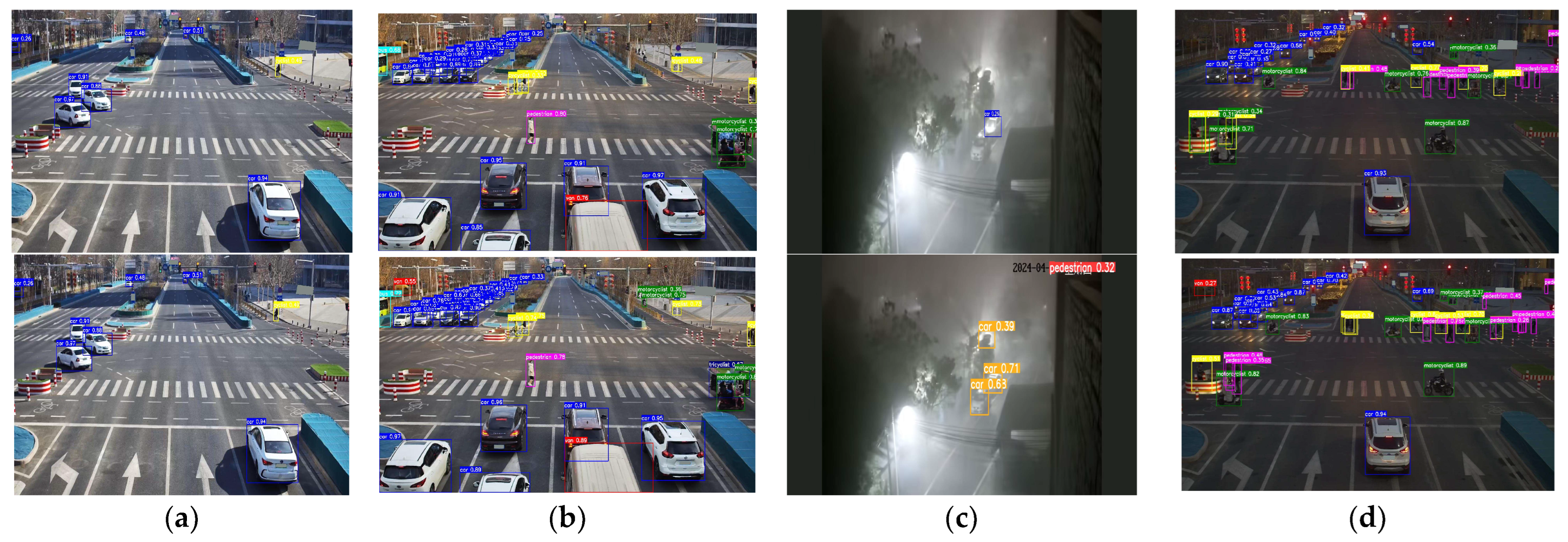
Figure A1 presents representative qualitative comparisons across off-peak, dense-traffic, inclement-weather, and nighttime scenes. The top row shows the baseline outputs and the bottom row shows the proposed configuration.
In these selected examples, the proposed configuration produces tighter boxes or retains additional detections in several crowded and low-light regions. The examples illustrate observed failure modes and improvements but do not quantify general weather robustness.
Figure A1. Supplementary qualitative comparison of detection results across four challenging intersection scenarios. The top row presents the baseline YOLOv8, and the bottom row shows results from the proposed configuration. (a) Off-peak period; (b) dense-traffic scenario; (c) inclement-weather condition; (d) nighttime environment.
Automation 07 00130 g0a1

References

  1. Caban, J.; Nieoczym, A.; Dudziak, A.; Krajka, T.; Stopka, O. The Planning Process of Transport Tasks for Autonomous Vans—Case Study. Appl. Sci. 2022, 12, 2993. [Google Scholar] [CrossRef] [Scilit]
  2. Paľo, J.; Caban, J.; Kiktová, M.; Černický, Ľ. The comparison of automatic traffic counting and manual traffic counting. IOP Conf. Ser. Mater. Sci. Eng. 2019, 710, 012041. [Google Scholar] [CrossRef] [Scilit]
  3. Wang, A.; Chen, H.; Liu, L.; Chen, K.; Lin, Z.; Han, J.; Ding, G. YOLOv10: Real-Time End-to-End Object Detection. Adv. Neural Inf. Process. Syst. 2024, 37, 107984–108011. [Google Scholar] [CrossRef] [Scilit]
  4. Rey, L.; Bernardos, A.M.; Dobrzycki, A.D.; Carramiñana, D.; Bergesio, L.; Besada, J.A.; Casar, J.R. A Performance Analysis of You Only Look Once Models for Deployment on Constrained Computational Edge Devices in Drone Applications. Electronics 2025, 14, 638. [Google Scholar] [CrossRef] [Scilit]
  5. Wojke, N.; Bewley, A.; Paulus, D. Simple Online and Realtime Tracking with a Deep Association Metric. In Proceedings of the 2017 IEEE International Conference on Image Processing (ICIP), Beijing, China, 17–20 September 2017; IEEE: New York, NY, USA, 2017; pp. 3645–3649. [Google Scholar] [CrossRef] [Scilit]
  6. Du, Y.; Zhao, Z.; Song, Y.; Zhao, Y.; Su, F.; Gong, T.; Meng, H. StrongSORT: Make DeepSORT Great Again. IEEE Trans. Multimed. 2023, 25, 8725–8737. [Google Scholar] [CrossRef] [Scilit]
  7. Bewley, A.; Ge, Z.; Ott, L.; Ramos, F.; Upcroft, B. Simple Online and Realtime Tracking. In Proceedings of the 2016 IEEE International Conference on Image Processing (ICIP), Phoenix, AZ, USA, 25–28 September 2016; IEEE: New York, NY, USA, 2016; pp. 3464–3468. [Google Scholar] [CrossRef] [Scilit]
  8. Rahi, A.; Wasfy, H.; Wasfy, T.; Anwar, S. Improved Object Detection and Tracking with Camera in Motion Using PrED: Predictive Enhancement of Detection. Automation 2025, 6, 77. [Google Scholar] [CrossRef] [Scilit]
  9. Li, H.; Peng, X.; Li, W.; Liu, Y.; Cai, G.; Sun, H. An Improved DeepSORT Algorithm for Multi-Target Posture Tracking of Firefighters. Automation 2026, 7, 93. [Google Scholar] [CrossRef] [Scilit]
  10. Li, S.; Yoon, H.-S. Sensor Fusion-Based Vehicle Detection and Tracking Using a Single Camera and Radar at a Traffic Intersection. Sensors 2023, 23, 4888. [Google Scholar] [CrossRef] [Scilit] [PubMed]
  11. Zhao, Y.; Lv, W.; Xu, S.; Wei, J.; Wang, G.; Dang, Q.; Liu, Y.; Chen, J. DETRs Beat YOLOs on Real-Time Object Detection. In Proceedings of the IEEE/CVF Conference on Computer Vision and Pattern Recognition (CVPR), Seattle, WA, USA, 17–21 June 2024; IEEE: New York, NY, USA, 2024; pp. 16965–16974. [Google Scholar]
  12. Ding, J.; Xue, N.; Long, Y.; Xia, G.-S.; Lu, Q. Learning RoI Transformer for Oriented Object Detection in Aerial Images. In Proceedings of the IEEE/CVF Conference on Computer Vision and Pattern Recognition (CVPR), Long Beach, CA, USA, 16–20 June 2019; IEEE: New York, NY, USA, 2019; pp. 2849–2858. [Google Scholar]
  13. Ye, X.; Shu, M.; Li, H.; Shi, Y.; Li, Y.; Wang, G.; Tan, X.; Ding, E. Rope3D: The Roadside Perception Dataset for Autonomous Driving and Monocular 3D Object Detection Task. In Proceedings of the IEEE/CVF Conference on Computer Vision and Pattern Recognition, New Orleans, LA, USA, 19–24 June 2022; IEEE: New York, NY, USA, 2022; pp. 21341–21350. [Google Scholar]
  14. Yang, M.; Yu, K.; Zhang, C.; Li, Z.; Yang, K. DenseASPP for Semantic Segmentation in Street Scenes. In Proceedings of the IEEE Conference on Computer Vision and Pattern Recognition, Salt Lake City, UT, USA, 18–22 June 2018; IEEE: New York, NY, USA, 2018; pp. 3684–3692. [Google Scholar]
  15. Liu, W.; Lu, H.; Fu, H.; Cao, Z. Learning to Upsample by Learning to Sample. In Proceedings of the IEEE/CVF International Conference on Computer Vision (ICCV), Paris, France, 1–6 October 2023; IEEE: New York, NY, USA, 2023; pp. 6027–6037. [Google Scholar] [CrossRef] [Scilit]
  16. Zhang, Y.; Wang, X.; Ye, X.; Zhang, W.; Lu, J.; Tan, X.; Ding, E.; Sun, P.; Wang, J. ByteTrackV2: 2D and 3D Multi-Object Tracking by Associating Every Detection Box. arXiv 2023, arXiv:2303.15334. [Google Scholar] [CrossRef] [Scilit]
  17. Zhang, Y.; Sun, P.; Jiang, Y.; Yu, D.; Weng, F.; Yuan, Z.; Luo, P.; Liu, W.; Wang, X. ByteTrack: Multi-Object Tracking by Associating Every Detection Box. In Computer Vision—ECCV 2022; Avidan, S., Brostow, G., Cissé, M., Farinella, G.M., Hassner, T., Eds.; Lecture Notes in Computer Science; Springer: Cham, Switzerland, 2022; Volume 13682, pp. 1–21. [Google Scholar] [CrossRef] [Scilit]
  18. Nørgaard, M.; Poulsen, N.K.; Ravn, O. New developments in state estimation for nonlinear systems. Automatica 2000, 36, 1627–1638. [Google Scholar] [CrossRef] [Scilit]
  19. Hartley, R.; Zisserman, A. Multiple View Geometry in Computer Vision, 2nd ed.; Cambridge University Press: Cambridge, UK, 2004. [Google Scholar] [CrossRef] [Scilit]
  20. Fischler, M.A.; Bolles, R.C. Random Sample Consensus: A Paradigm for Model Fitting with Applications to Image Analysis and Automated Cartography. Commun. ACM 1981, 24, 381–395. [Google Scholar] [CrossRef] [Scilit]
  21. Lowe, D.G. Distinctive image features from scale-invariant keypoints. Int. J. Comput. Vis. 2004, 60, 91–110. [Google Scholar] [CrossRef] [Scilit]
  22. Liao, B.; Chen, S.; Wang, X.; Cheng, T.; Zhang, Q.; Liu, W.; Huang, C. MapTR: Structured Modeling and Learning for Online Vectorized HD Map Construction. In Proceedings of the Eleventh International Conference on Learning Representations (ICLR), Kigali, Rwanda, 1–5 May 2023. [Google Scholar]
  23. Liao, B.; Chen, S.; Zhang, Y.; Jiang, B.; Zhang, Q.; Liu, W.; Huang, C.; Wang, X. MapTRv2: An End-to-End Framework for Online Vectorized HD Map Construction. Int. J. Comput. Vis. 2025, 133, 1352–1374. [Google Scholar] [CrossRef] [Scilit]
  24. Liu, Z.; Tang, H.; Amini, A.; Yang, X.; Mao, H.; Rus, D.; Han, S. BEVFusion: Multi-Task Multi-Sensor Fusion with Unified Bird’s-Eye View Representation. In Proceedings of the 2023 IEEE International Conference on Robotics and Automation (ICRA), London, UK, 29 May–2 June 2023; IEEE: New York, NY, USA, 2023; pp. 2774–2781. [Google Scholar]
  25. Yang, C.; Chen, Y.; Tian, H.; Tao, C.; Zhu, X.; Zhang, Z.; Huang, G.; Li, H.; Qiao, Y.; Lu, L.; et al. BEVFormer v2: Adapting Modern Image Backbones to Bird’s-Eye-View Recognition via Perspective Supervision. In Proceedings of the IEEE/CVF Conference on Computer Vision and Pattern Recognition (CVPR), Vancouver, BC, Canada, 18–22 June 2023; IEEE: New York, NY, USA, 2023; pp. 17830–17839. [Google Scholar]
  26. Hu, J.; Shen, L.; Albanie, S.; Sun, G.; Wu, E. Squeeze-and-Excitation Networks. IEEE Trans. Pattern Anal. Mach. Intell. 2020, 42, 2011–2023. [Google Scholar] [CrossRef] [Scilit] [PubMed]
  27. Tong, Z.; Chen, Y.; Xu, Z.; Yu, R. Wise-IoU: Bounding Box Regression Loss with Dynamic Focusing Mechanism. arXiv 2023, arXiv:2301.10051. [Google Scholar] [CrossRef] [Scilit]
  28. Lau, K.W.; Po, L.M.; Rehman, Y.A.U. Large Separable Kernel Attention: Rethinking the Large Kernel Attention Design in CNN. Expert Syst. Appl. 2024, 236, 121352. [Google Scholar] [CrossRef] [Scilit]
  29. Wen, L.; Du, D.; Cai, Z.; Lei, Z.; Chang, M.-C.; Qi, H.; Lim, J.; Yang, M.-H.; Lyu, S. UA-DETRAC: A New Benchmark and Protocol for Multi-Object Detection and Tracking. Comput. Vis. Image Underst. 2020, 193, 102907. [Google Scholar] [CrossRef] [Scilit]
  30. Zhu, P.; Wen, L.; Du, D.; Bian, X.; Fan, H.; Hu, Q.; Ling, H. Detection and Tracking Meet Drones Challenge. IEEE Trans. Pattern Anal. Mach. Intell. 2022, 44, 7380–7399. [Google Scholar] [CrossRef] [Scilit] [PubMed]
  31. Yu, F.; Chen, H.; Wang, X.; Xian, W.; Chen, Y.; Liu, F.; Madhavan, V.; Darrell, T. BDD100K: A Diverse Driving Dataset for Heterogeneous Multitask Learning. In Proceedings of the IEEE/CVF Conference on Computer Vision and Pattern Recognition (CVPR), Seattle, WA, USA, 13–19 June 2020; IEEE: New York, NY, USA, 2020; pp. 2633–2642. [Google Scholar] [CrossRef] [Scilit]
  32. Bibbo’, L.; Bilotta, G.; Angiulli, G. High-Density PCB for On-Edge AI: Energy Harvesting, Thermal Management, and Sensor Fusion for UAVs in Clinical–Urban Missions. Electronics 2026, 15, 1885. [Google Scholar] [CrossRef] [Scilit]
  33. Oyebamiji, O.; Dissanayake, D.; Cavus, M. Enhancing Uncertainty Estimation with Deep Gaussian Processes. In Proceedings of the UK AI Conference 2024, Birmingham, UK, 22 November 2024; Benford, A., Cabrera, C., Kiden, S., Salili-James, A., Zakka, V.G., Eds.; Proceedings of Machine Learning Research; PMLR: Cambridge, MA, USA, 2025; Volume 295, pp. 26–42. [Google Scholar]
  34. Woo, S.; Park, J.; Lee, J.-Y.; Kweon, I.S. CBAM: Convolutional Block Attention Module. In Computer Vision—ECCV 2018; Ferrari, V., Hebert, M., Sminchisescu, C., Weiss, Y., Eds.; Lecture Notes in Computer Science; Springer International Publishing: Cham, Switzerland, 2018; Volume 11211, pp. 3–19. [Google Scholar] [CrossRef] [Scilit]
  35. Wang, Q.; Wu, B.; Zhu, P.; Li, P.; Zuo, W.; Hu, Q. ECA-Net: Efficient Channel Attention for Deep Convolutional Neural Networks. In Proceedings of the IEEE/CVF Conference on Computer Vision and Pattern Recognition, Seattle, WA, USA, 13–19 June 2020; IEEE: New York, NY, USA, 2020; pp. 11531–11539. [Google Scholar] [CrossRef] [Scilit]
  36. Liu, Y.; Shao, Z.; Teng, Y.; Hoffmann, N. NAM: Normalization-Based Attention Module. arXiv 2021, arXiv:2111.12419. [Google Scholar] [CrossRef] [Scilit]
  37. Jiao, J.; Tang, Y.-M.; Lin, K.-Y.; Gao, Y.; Ma, A.J.; Wang, Y.; Zheng, W.-S. DilateFormer: Multi-Scale Dilated Transformer for Visual Recognition. IEEE Trans. Multimed. 2023, 25, 8906–8919. [Google Scholar] [CrossRef] [Scilit]
  38. He, K.; Zhang, X.; Ren, S.; Sun, J. Spatial Pyramid Pooling in Deep Convolutional Networks for Visual Recognition. IEEE Trans. Pattern Anal. Mach. Intell. 2015, 37, 1904–1916. [Google Scholar] [CrossRef] [Scilit] [PubMed]
  39. Li, C.; Li, L.; Geng, Y.; Jiang, H.; Cheng, M.; Zhang, B.; Ke, Z.; Xu, X.; Chu, X. YOLOv6 v3.0: A Full-Scale Reloading. arXiv 2023, arXiv:2301.05586. [Google Scholar] [CrossRef] [Scilit]
  40. Wang, J.; Chen, K.; Xu, R.; Liu, Z.; Loy, C.C.; Lin, D. CARAFE: Content-Aware ReAssembly of FEatures. In Proceedings of the IEEE/CVF International Conference on Computer Vision, Seoul, Republic of Korea, 27 October–2 November 2019; IEEE: New York, NY, USA, 2019; pp. 3007–3016. [Google Scholar] [CrossRef] [Scilit]
  41. Lu, H.; Liu, W.; Fu, H.; Cao, Z. FADE: Fusing the Assets of Decoder and Encoder for Task-Agnostic Upsampling. In Computer Vision—ECCV 2022; Springer: Cham, Switzerland, 2022; Volume 13687, pp. 231–247. [Google Scholar] [CrossRef] [Scilit]
  42. Ren, S.; He, K.; Girshick, R.; Sun, J. Faster R-CNN: Towards Real-Time Object Detection with Region Proposal Networks. IEEE Trans. Pattern Anal. Mach. Intell. 2017, 39, 1137–1149. [Google Scholar] [CrossRef] [Scilit] [PubMed]
  43. Xie, X.; Cheng, G.; Wang, J.; Yao, X.; Han, J. Oriented R-CNN for Object Detection. In Proceedings of the 2021 IEEE/CVF International Conference on Computer Vision (ICCV), Montreal, QC, Canada, 10–17 October 2021; IEEE: New York, NY, USA, 2021; pp. 3500–3509. [Google Scholar] [CrossRef] [Scilit]
  44. Jocher, G.; Chaurasia, A.; Stoken, A.; Borovec, J.; Kwon, Y.; Michael, K.; Fang, J.; Yifu, Z.; Wong, C.; Montes, D.; et al. ultralytics/yolov5: v7.0—YOLOv5 SOTA Realtime Instance Segmentation; Zenodo: Geneva, Switzerland, 2022. [Google Scholar] [CrossRef]
  45. Jocher, G.; Chaurasia, A.; Qiu, J. Ultralytics YOLOv8, Version 8.0.0. Computer Software. 2023. Available online: https://github.com/ultralytics/ultralytics (accessed on 6 August 2026).
  46. Wang, C.-Y.; Yeh, I.-H.; Liao, H.-Y.M. YOLOv9: Learning What You Want to Learn Using Programmable Gradient Information. In Computer Vision—ECCV 2024; Leonardis, A., Ricci, E., Roth, S., Russakovsky, O., Sattler, T., Varol, G., Eds.; Lecture Notes in Computer Science; Springer Nature Switzerland: Cham, Switzerland, 2025; Volume 15089, pp. 1–21. [Google Scholar] [CrossRef] [Scilit]
  47. Jocher, G.; Qiu, J. Ultralytics YOLO11, Version 11.0.0. Computer Software. 2024. Available online: https://github.com/ultralytics/ultralytics (accessed on 6 August 2026).
  48. Tian, Y.; Ye, Q.; Doermann, D. YOLOv12: Attention-Centric Real-Time Object Detectors. Adv. Neural Inf. Process. Syst. 2025, 38, 78433–78457. [Google Scholar]
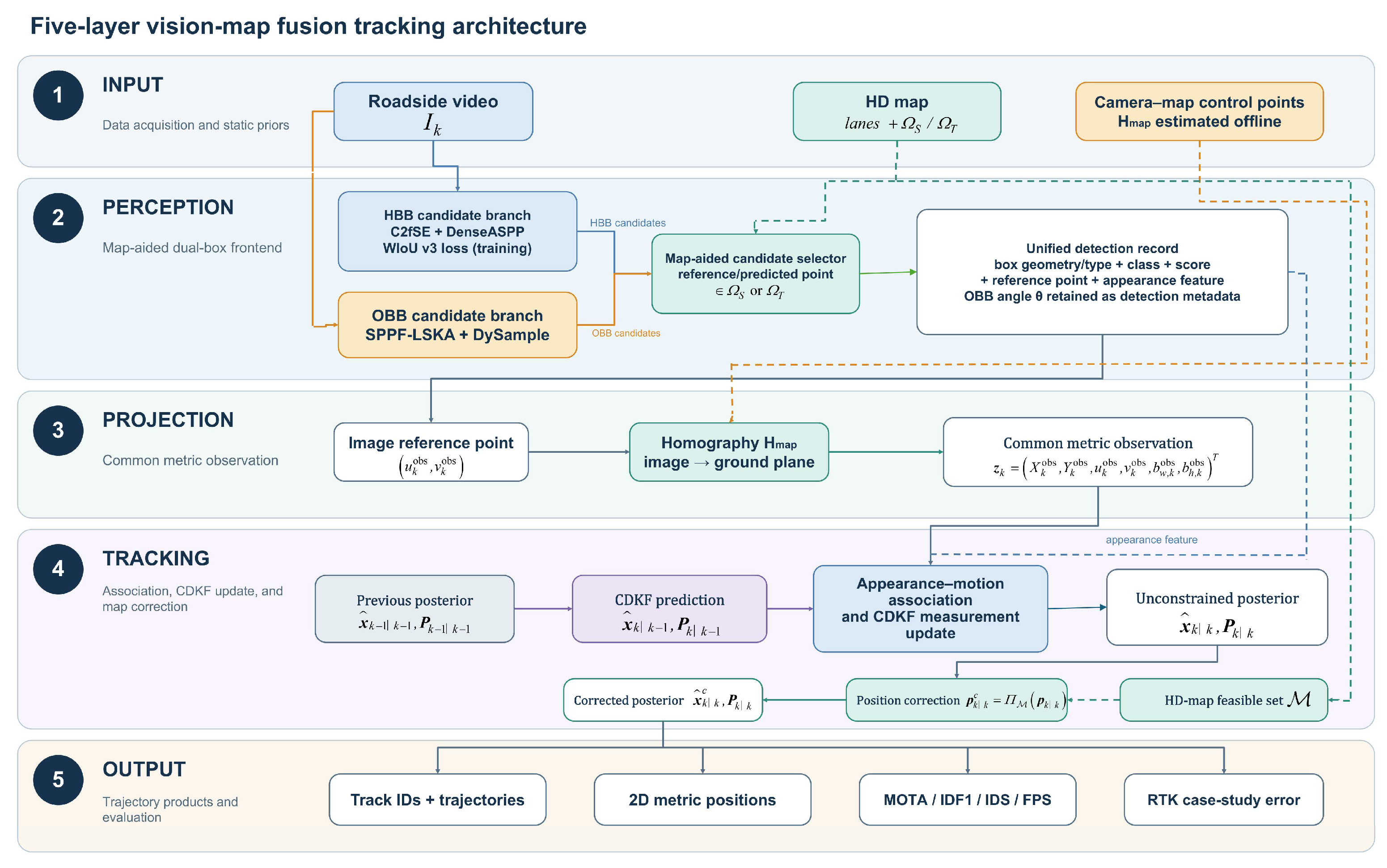
Figure 1. Five-layer architecture of the fixed-camera vision-map fusion tracking framework.
Automation 07 00130 g001
Figure 2. Data flow of the map-aided dual-box frontend and constrained CDKF backend.
Automation 07 00130 g002
Figure 3. Qualitative comparison of detection results in complex intersection scenarios. The top row represents the baseline YOLOv8, and the bottom row presents the proposed algorithm. (a) Turning scenarios; (b) dense target scenarios; (c) nighttime scenarios.
Automation 07 00130 g003
Figure 4. Hardware deployment of the real-world intersection experimental environment. (a) Roadside high-definition camera installation; (b) edge computing device for real-time perception; (c) roof-mounted global navigation satellite system (GNSS) antenna; (d) Beiyun X1 high-precision RTK terminal.
Automation 07 00130 g004
Figure 5. Qualitative comparative analysis of spatial trajectories. (ac) Trajectory tracking performance in straight-driving scenarios; (df) trajectory tracking performance under complex turning maneuvers.
Automation 07 00130 g005
Figure 6. Lateral-position trajectories from the proposed vision-based localization method and the Beiyun RTK reference over the displayed 0–80 m trajectory segment.
Automation 07 00130 g006
Table 1. Ablation experiments of the HBB branch in the straight-driving region (evaluated on the UA-DETRAC dataset).
ModelC2fSEDENSEASPPWIoU v3Precision (%)Recall (%)mAP@0.5 (%)mAP0.5–0.95 (%)
Baseline 96.796.398.988.6
+C2fSE 97.596.798.788.8
+DenseASPP 96.196.998.888.3
Proposed96.998.099.189.1
Table 2. Sequential ablation of the OBB branch on Rope3D; intermediate rows need not improve every metric.
ModelLSKADySamplePrecision (%)Recall (%)mAP@0.5 (%)mAP0.5–0.95 (%)
Baseline 82.966.874.941.7
+LSKA 84.066.174.740.7
Proposed85.666.875.642.7
Table 3. End-to-end tracking comparison. Detector and association configurations were not fully harmonized; values should not be interpreted as a filter-only ablation.
TrackerTracking BackendMOTA(↑)MOTP(↑)IDF1(↑)IDS(↓)FPS
SORTLinear KF61.4%72.1%71.1%142139.6
DeepSORTLinear KF70.8%78.3%78.4%78425.2
StrongSORTLinear KF70.4%78.2%81.2%67413.4
ProposedCDKF + Map Prior74.5%80.2%82.6%61426.8
Table 4. Descriptive localization MAE for the single-vehicle, single-intersection case study; configurations differ in multiple components (m).
MethodBox RepresentationSpatial ConstraintOverall MAE (m)
Baseline end-to-end configurationHBBUnconstrained 2D0.208
Proposed end-to-end configurationOBBHD-map feasible-set projection0.180
Disclaimer/Publisher’s Note: The statements, opinions and data contained in all publications are solely those of the individual author(s) and contributor(s) and not of MDPI and/or the editor(s). MDPI and/or the editor(s) disclaim responsibility for any injury to people or property resulting from any ideas, methods, instructions or products referred to in the content.