


Highlights
What are the main findings?
- The AI-integrated pipeline surpassed traditional methods (SOR, density filters, RANSAC, CloudCompare) in upper-layer reconstruction and uncertainty calibration, achieving ECE < 0.05. Ablation studies confirmed the essential roles of physics-aware losses and multi-modal fusion, while demonstrating linear scalability to 50,000 points.
- The framework delivered three key innovations: (i) a 50-dimensional geometric descriptor achieving near-perfect blob–noise separation (RQ1), (ii) a physics-aware VAE enhancing upper-layer density by 28.7% via inverse-square law constraints (RQ2), and (iii) height-stratified uncertainty decomposition yielding well-calibrated uncertainty maps (ECE ≈ 0.04, RQ3).
What are the implications of the main findings?
- These results demonstrate that physics-aware AI pipelines enable reliable automated inspection of tall structures from sparse LiDAR data with calibrated uncertainty, allowing engineers to prioritize uncertain regions and deploy scalable monitoring systems in practice.
- Embedding physical laws and domain-specific features into deep learning proves highly effective for vertically stratified, sparse data—opening pathways for physics-informed models in drone LiDAR, atmospheric sensing, and other distance-dependent remote sensing applications.
Abstract
High-rise LiDAR scanning produces vertically sparse point clouds where upper-layer defects are hardest to detect due to inverse-square ranging law (1/r2) density gradients, noise contamination, and complex geometries. This paper presents PC-TowerNet, a physics-aware AI pipeline that achieves state-of-the-art reconstruction through sequential modules: (1) 50D geometric feature classification outperforming CloudCompare SOR (100% accuracy vs. 91.3% retention); (2) Physics-Constrained VAE (PC-VAE) recovering 28.7 ± 2.1% upper density vs. 8.3 ± 1.7% standard VAE; (3) multi-modal PointNet++/GNN/Transformer fusion; and (4) Bayesian uncertainty maps (ECE = 0.042 ± 0.008). Synthetic tower evaluation (10 × 5 seeds) demonstrates 48.9% surface smoothness improvement and 38.2% volume error reduction over tuned RANSAC baselines, with clear paths to real-data validation.
1. Introduction
Regular structural inspection of high-rise infrastructure (telecommunication towers, chimneys, skyscrapers) drives LiDAR adoption for 3D digital twins and damage assessment. However, ground-based scanning introduces critical challenges: (1) vertical density gradients from inverse-square ranging create 40–60% upper-layer sparsity where defects are hardest to detect; (2) environmental noise/outlier corrupt geometric analysis; (3) tapered/lattice geometries defy simple primitive fitting; and (4) missing uncertainty estimates undermine risk-aware decisions.
Prior analyses by the authors revealed that ground-based LiDAR scanning of high-rise infrastructure creates vertical density gradients (1/r2 law), leading to 40–60% sparsity in upper layers where defects are critical yet hardest to detect. Environmental noise and tapered lattice geometries further corrupt primitive fitting (e.g., RANSAC failures), while absent probabilistic guarantees hinder risk assessment. The core problem is the lack of physics-aware, uncertainty-quantified pipelines tailored to towers, as general methods (PointNet++, CloudCompare SOR) fail under height-sparse conditions [1,2].
This work investigates three questions: RQ1: Can compound-scaled geometric features outperform SOR for blob–noise separation? RQ2: Does embedding 1/r2 physics in VAE loss restore density? RQ3: Does Bayesian multi-modal fusion beat RANSAC for uncertainty-aware reconstruction? Contributions include: (1) PC-VAE with physics loss, (2) 50D classifier, (3) height-stratified uncertainty, (4) CloudCompare ablations, and (5) end-to-end tower pipeline.
The paper is organized as follows:
Section 2 reviews traditional and deep learning methods, positioning the proposed physics-aware integration. Section 3 details each module with clarified notation and theoretical grounding. Section 4 justifies synthetic dataset design, parameters, and metrics. Section 5 presents quantitative results and ablation studies. Section 6 acknowledges synthetic-data limits and outlines real LiDAR validation. This structure ensures each claim traces directly from problem definition to empirical support.
2. Related Works
2.1. Traditional Point Cloud Processing
Point cloud processing has evolved significantly since the early days of photogrammetric techniques. Traditional methods can be categorized into three main approaches:
Geometric Primitive Fitting: RANSAC (Fischler & Bolles, 1981) remains the gold standard for robust geometric fitting, despite its computational cost [3]. Schnabel et al. extended RANSAC for efficient primitive detection, including cylinders, spheres, and cones [4]. However, these methods struggle with complex structures that cannot be decomposed into simple primitives.
Surface Reconstruction: Poisson reconstruction [5] formulates surface extraction as the solution of a Poisson equation, producing smooth surfaces but requiring oriented normals. The Ball-Pivoting Algorithm [6] grows triangulations from seed triangles and is suitable for dense, uniform data, but it performs poorly under variable density conditions. Alpha shapes [7] provide topologically correct reconstructions but require careful parameter selection.
Statistical Filtering: SOR [8] removes points whose k-nearest-neighbor distances exceed statistical thresholds. Radius Outlier Removal (ROR) eliminates isolated points within a specified radius. These methods are computationally efficient but lack semantic understanding of structural content versus noise.
Limitations: Traditional methods share several common limitations: (1) heavy reliance on manual parameter tuning, (2) inability to learn from data, (3) lack of uncertainty quantification, (4) poor handling of variable density, and (5) limited adaptability to different structure types.
2.2. Deep Learning for Point Clouds
The introduction of revolutionized point cloud deep learning by directly processing unordered point sets through symmetric functions. PointNet++/ extended this idea with hierarchical feature learning via Farthest Point Sampling (FPS) and Set Abstraction layers, enabling multi-scale representation.
In terms of architectural evolution, related works include PointCNN [9], which learns a χ-transformation for canonical ordering; DGCNN [10], which uses dynamic graph construction to capture local geometry; Point Transformer [11], which introduces self-attention mechanisms to model long-range dependencies; and various extensions of PointNet++ that improve sampling, grouping, and feature aggregation.
Generative-model-based approaches include PointFlow [12], which uses continuous normalizing flows for point cloud generation; Point Cloud VAE [13], which applies variational autoencoders to 3D shape completion; and PointGrow [14], which enables autoregressive generation for missing regions.
Graph neural network–based methods include DGCNN with EdgeConv for learning edge features; Point-GNN [15], which focuses on graph construction for 3D object detection; and Point Cloud GCN [16], which leverages spectral graph convolutions.
For uncertainty quantification, relevant works include Bayesian PointNet [17], which provides dropout-based uncertainty estimates for classification; Deep Ensembles [18], which relies on multiple model predictions; and Evidential Deep Learning [19], which incorporates evidential reasoning into uncertainty estimation.
Research gap: Despite significant progress, no existing work specifically addresses high-rise structure processing with: (1) physics-aware density compensation, (2) an integrated multi-architecture framework, (3) comprehensive uncertainty quantification, or (4) a systematic comparison with industry tools.
2.3. EfficientNet and Compound Scaling
EfficientNet [20] introduced compound scaling, which uniformly scales network depth, width, and resolution according to the following equations:
where α · β2 · γ2 ≈ 2, and φ is the compound coefficient.
depth: d = αφ
width: w = βφ
resolution: r = γφ
The Mobile Inverted Bottleneck Convolution (MBConv) block with Squeeze-and-Excitation (SE) [21] provides efficient feature extraction. Although originally designed for 2D images, these principles have not yet been systematically applied to 3D point cloud classification.
2.4. CloudCompare and Industry Tools
CloudCompare [22] is the de facto open-source standard for point cloud processing. It offers SOR via k-NN distance thresholding, density-based filtering through radius-neighbor counting, RANSAC-based shape detection for primitive fitting, and distance computation for cloud-to-cloud and cloud-to-mesh comparisons. Other industry tools include Autodesk ReCap, Leica Cyclone, and Bentley ContextCapture, which excel at interactive processing but lack automated learning capabilities.
2.5. The Advance of the Proposed Method
Several works have addressed infrastructure-specific challenges, including bridge inspection using deep learning for crack detection; building facades with RANSAC-based plane extraction; power lines [4] via hierarchical clustering However, high-rise structures remain underexplored, particularly in terms of vertical density compensation and integrated AI-based approaches. Table 1 summarizes how the proposed method advances beyond prior work.
Table 1.
The advance of the proposed method.
Point cloud processing has evolved significantly since early photogrammetric techniques. It is categorized traditional methods into three main approaches:
Geometric Primitive Fitting: RANSAC remains the gold standard for robust geometric fitting despite its computational cost. Schnabel et al. extended RANSAC for efficient primitive detection including cylinders, spheres, and cones. However, these methods struggle with complex structures that cannot be decomposed into simple primitives. This table directly addresses the three research questions (RQ1–3) from the manuscript introduction. It contrasts traditional statistical methods (SOR [8], Poisson [5]) and infrastructure-specific approaches (bridges, power lines) with PC-TowerNet’s innovations: semantic feature engineering for perfect blob–noise separation, physics-constrained generative densification, and the first integrated pipeline for high-rise tower scanning with uncertainty quantification.
Range image technique for change detection of rock slopes using dense point cloud data was proposed [23]. It is applicable to “Bridge” of height-stratified tower pipeline as is shown in Table 1. Also, classification of airborne laser scanning data using JointBoost was proposed as shown in Table 1 [24].
2.6. Point Cloud Processing for Infrastructure
As references to major advancements in LiDAR processing and point cloud learning since 2020, the following outlines current research trends in terms of point cloud representation learning, segmentation, transformer applications, and generative models. Furthermore, recent major technological advancements such as efficient processing of large point clouds, geometric feature extraction using graph neural networks, and global contextual understanding using transformers are also listed below.
Point Transformer and Point Transformer Networks for LiDAR 3D Object Detection were proposed. Also, Point-GNN: Graph Neural Network for 3D Object Detection in a Point Cloud is proposed. On the other hand, Dynamic Graph CNN for Learning on Point Clouds was proposed. This document has been widely cited as a standard foundation for point cloud learning since 2020. Autoregressive Neural Point Cloud Generation called “PointGrow” was proposed. Efficient Semantic Segmentation of Large-Scale Point Clouds called “RandLA-Net” was also proposed. PointNet: deep energy-based learning on unordered point sets for 3D generation was proposed for reconstruction and classification [25]. Physics-informed machine learning was discussed as a survey on problems for methods and applications [26]. Scientific machine learning through physics-informed neural networks were also discussed [27].
2.7. Physics-Informed Machine Learning (PIML) and Physics-Guided Machine Learning (PGML)
The following are key papers and surveys on Physics-Informed Machine Learning (PIML) and Physics-Guided Machine Learning (PGML).
A Deep Learning Framework for Solving Forward and Inverse Problems Involving Nonlinear Partial Differential Equations called “Physics-Informed Neural Networks” was proposed [28]. Meanwhile, “Physics-Informed Machine Learning” was proposed [29]. Survey report was issued with surveyed problems, methods and applications for “Physics-Informed Machine Learning” [26]. A Taxonomy and Survey of Integrating Knowledge into Learning Systems for Informed Machine Learning was also issued [30]. Meantime, recent progress and future opportunities in full-waveform inversion on Physics-Guided Data-Driven Seismic Inversion was reviewed [31]. A Deep Learning Algorithm for Solving Partial Differential Equations was proposed [32].
These publications cover a wide range of topics, from methods for incorporating partial differential equations (PDEs) as constraints into neural networks to frameworks for integrating broader physical knowledge into learning systems. In particular, PINNs is the most widely cited foundational research in the current field of PIML.
3. Proposed Method
This section presents a comprehensive AI-integrated framework for high-rise structure point cloud processing. It emphasizes the novel components of the proposed method and their theoretical foundations. First, the notation used throughout the method is summarized. Let denote the input point cloud, where each point is represented in a global Cartesian coordinate system. Let denote height, and let be partitioned into horizontal layers using fixed-height bins for density estimation and reconstruction. For each local patch , the covariance matrix and its ordered eigenvalues are computed and used to define linearity, planarity, and sphericity, as introduced in Section 3.2. Unless otherwise noted, all expectations and variances are taken with respect to the predictive distribution of the corresponding Bayesian model.
3.1. System Architecture Overview
The proposed framework consists of five main components arranged in sequence: raw point cloud input, blob classification using an EfficientNet-inspired classifier, multi-modal feature extraction using PointNet++ [23], graph neural networks, and transformers, physics-aware densification using a variational autoencoder, uncertainty quantification using Bayesian deep learning, and surface reconstruction, which together produce a 3D model with an uncertainty map. Each component is described in detail below.
3.2. EfficientNet-Inspired Blob Classifier
3.2.1. Motivation and Novelty
Traditional noise removal methods lack semantic understanding of structure versus noise. This study proposes the first application of EfficientNet’s compound scaling principles to point cloud patch classification, achieving perfect accuracy through carefully engineered features. A key contribution is the integration of geometric feature engineering with deep learning architecture principles for 3D data.
3.2.2. Feature Engineering
A 50-dimensional set of geometric features is extracted from local point patches. These include:
- (1)
- Statistical features (12D), defined as
- (2)
- The PCA features from local patch covariance matrix yield sorted eigenvalues , defining:
Enhanced Algorithm (Algorithm 1) Steps are as follows:
| Algorithm 1: PC-TowerNet Pipeline |
Input: Raw point cloud , Output: Surface , uncertainty
|
This expands the original pseudocode with explicit feature extraction and physics checks.
- (3)
- Density features (3D), where -nearest-neighbor average distances capture local density:
- (4)
- Shape descriptors, including volume, aspect ratio, and radial variance.
A notable aspect of this feature set is that it provides perfect linear separability between blobs and noise, as validated by experiments showing 100% accuracy with simple logistic regression.
3.2.3. MBConv Block Adaptation
EfficientNet’s Mobile Inverted Bottleneck Convolution (MBConv) block is adapted for point cloud features as follows. Given input of shape , the features are first expanded by a convolution with expansion ratio 6, producing . This is followed by depth-wise point-wise processing, squeeze-and-excitation channel attention, and projection through another convolution to . A skip connection is applied when , yielding the final output.
The SE block, which is novel in this point cloud setting, consists of squeeze via global average pooling to (1,C), excitation to obtain channel importance weights , and scaling by reweighting the channels. Where (1,C) represents the tensor shape in the SE (Squeeze-and-Excitation) block of the point cloud processing. It indicates that the global average pooling result after the squeeze operation has the shape (1,C) for a batch size of 1 (single sample) and number of channels C. A key contribution is the first application of SE attention to point cloud geometric features, allowing the model to learn feature importance automatically.
3.2.4. Compound Scaling for Point Clouds
The EfficientNet scaling principle is extended to point cloud processing through a depth multiplier for network layers, a width multiplier for feature dimensions, and a resolution multiplier for sampling density. This systematic scaling strategy for point cloud architectures is a novel contribution that has not been previously explored in the literature.
3.3. Physics-Aware VAE Densification
3.3.1. Problem Formulation
LiDAR scanning from ground level follows an inverse-square law, which produces a substantial density decrease in upper layers and can reduce reconstruction quality by 40–60%.
3.3.2. VAE Architecture
A standard VAE for point clouds operates as follows: in the encoder, the input is mapped to latent variables and via the reparameterization trick; in the decoder, the point cloud is reconstructed from the latent representation; and the standard objective combines reconstruction loss and KL divergence.
3.3.3. Physics-Guided Generation
The proposed physics-guided generation augments the VAE loss with physics-based constraints. Here, the total loss is defined as
where is based on a physics model and controls its influence. The target generation count is defined accordingly.
A key contribution is the first integration of physical measurement laws into generative models for point clouds, guiding generation to respect scanner physics while preserving geometric plausibility through KL regularization. Theoretical justification follows from the fact that physics priors structure the latent space, allowing interpolation to produce physically plausible points rather than arbitrary samples.
3.4. Multi-Modal Feature Integration
3.4.1. PointNet++ Hierarchical Features
PointNet++ is used for multi-scale local feature extraction through set abstraction layers. Farthest point sampling is applied first, followed by grouping around each centroid using neighborhood queries, and then local features are extracted with PointNet and aggregated by max pooling. This is organized into a three-level hierarchy: Level 1 with radius 10 m and for coarse structure, Level 2 with radius 5 m and for medium-scale details, and Level 3 with radius 2 m and for fine features. A novel aspect is adaptive radius selection based on local density, which addresses variable point spacing in high-rise structures.
3.4.2. Graph Neural Network Structure Learning
Graph construction is defined so that each point is connected to its neighbors, and the edge features encode relative position, distance, and direction. Message passing is then performed over this graph, and the structure score is computed from the resulting embeddings. A novel aspect is the integration of local density with graph features for robust structure identification in sparse regions.
3.4.3. Transformer Global Context
Three-dimensional positional encoding is combined with height-aware weighting to emphasize vertical coherence. Multi-head self-attention is then applied to model long-range dependencies. A novel idea is the use of height-prioritized positional encoding, which emphasizes vertical structural consistency and is especially important for high-rise structures.
3.4.4. Feature Fusion
The integrated representation is expressed as
where denotes PointNet++ hierarchical features, denotes Transformer attention features, and denotes graph neural network message-passing features. A key contribution is the first principled multi-modal fusion framework for point cloud processing, combining complementary feature types.
3.5. Bayesian Uncertainty Quantification
3.5.1. Monte Carlo Dropout
Monte Carlo dropout is adapted for point clouds. During inference, dropout is applied multiple times for stochastic forward passes, and the resulting predictions are collected for uncertainty estimation. The predictive mean and variance are then computed from these samples.
3.5.2. Uncertainty Decomposition
Epistemic uncertainty, which reflects model uncertainty, is estimated from the variability of predictions across Monte Carlo dropout samples. Aleatoric uncertainty, which reflects data noise, is estimated from the average predictive variance. Their sum yields the total uncertainty. A novel feature of this framework is height-stratified uncertainty estimation, which captures the increased epistemic uncertainty in sparse upper layers.
3.5.3. Calibration Metrics
Calibration quality is measured using Expected Calibration Error (ECE). The experiments achieve ECE below 0.05, indicating well-calibrated predictions.
3.6. Surface Reconstruction
For surface reconstruction, a cylindrical-aware method is adopted. For each height layer , the layer points are extracted, the convex hull in the plane is computed, and the points are converted to polar coordinates using a central reference point. Angles and radii are then used for smooth interpolation, followed by Gaussian filtering, and the final surface is reconstructed from the smoothed representation. A novel aspect is the combination of convex hull computation and polar smoothing, which provides robust reconstruction for cylindrical structures while resisting outliers.
3.7. Algorithm Summary
The complete AI-integrated point cloud processing pipeline takes a raw point cloud as input and produces a reconstructed surface and uncertainty map as output. The procedure is as follows: first, blob classification is performed by extracting features from each patch in and labeling them, resulting in classified patches; second, multi-modal feature extraction is conducted to obtain PointNet++, Transformer, and GNN features, which are then fused; third, physics-aware densification is applied layer by layer, generating additional points where necessary and updating the point cloud; fourth, uncertainty quantification is performed through multiple stochastic forward passes; and finally, the reconstructed surface and uncertainty map are returned.
Following standard Bayesian formulations, the total predictive uncertainty is decomposed into epistemic and aleatoric components. Epistemic uncertainty captures model uncertainty and is estimated from the variability of predictions across Monte Carlo dropout samples, whereas aleatoric uncertainty arises from data noise and is estimated from the average predictive variance. Their sum yields the total uncertainty, which is reported as a height-stratified profile along the tower.
The detailed PC-TowerNet Pipeline algorithms (Algorithm 2) are as follows:
| Algorithm 2: PC-TowerNet Pipeline |
| Input: Raw point cloud P = {pi}{i=1}N, pi = (xi, yi, zi) Output: Reconstructed surface S, uncertainty map U 1. BLOB_CLASSIFICATION(P): | for patch ∈ extract_patches(P, radius = 2 m): | features ← extract_50D_features(patch) | label ← EfficientNet(features) # 100% accuracy | Pblob ← P[label == "blob"] | return Pblob 2. MULTI_MODAL_FEATURES(P_blob): | Flocal ← PointNet++(Pblob, radii = [10 m, 5 m, 2 m]) | Fstruct ← GNN(Pblob, k = 20, layers = 3) | Fglobal ← Transformer(Pblob, heads = 4, wz = 2.0) | Ffused ← αFlocal + βFstruct + γFglobal # α + β + γ = 1 | return Ffused 3. PHYSICS_VAE_DENSIFICATION(Pblob): | for layer z ∈ height_bins(Pblob): | ρactual ← count(Pblob[z])/volume(z) | ρexpected ← ρ0 × (z0/z)2 # 1/r2 physics prior | if ρactual < ρexpected: | Pnew ← PC_VAE(Pblob[z], β = 0.001, γ = 0.1) | Pblob ← Pblob ∪ Pnew | return Pblob 4. BAYESIAN_UNCERTAINTY(S): | for t = 1 to T = 30: # MC Dropout | St ← surface_reconstruction(Pblob, dropout = 0.1) | S ← mean({St}) | Uepistemic ← Varθ[E[y|x,θ]] | Ualeatoric ← Eθ[Var[y|x,θ]] | Utotal ← Uepistemic + Ualeatoric | return S, Utotal 5. return surface_reconstruction(Pblob), Utotal |
Figure 1 shows PC-TowerNet Pipeline Block Diagram. The diagram shows process flow and the number of points.
Figure 1.
PC-TowerNet Pipeline Block Diagram.
The main processing flow is as follows: Raw LiDAR (3282 points) → 50D blob filtering (2601 points, 20.7% reduction) → Feature fusion using PointNet + GNN + Transformer → Physically constrained VAE densification (3362 points, upper layer +29.3%) → Bayesian uncertainty quantification (ECE = 0.042) → Cylinder-aware surface reconstruction (S, U_total output).
4. Experiment
All experiments in this study are conducted on controlled synthetic towers, which allow us to systematically vary height, radius, noise level, and sparsification while preserving ground-truth geometry. However, this design also limits the immediate generalizability of the findings, because real-world LiDAR scans may contain additional artifacts such as occlusions, mixed materials, and scanner-specific noise patterns that are not fully captured by the proposed generator. Therefore, the current evaluation should be regarded as a necessary first step: it isolates and tests the behavior of each component under known physical parameters, but it does not replace validation on real LiDAR datasets. As future work, the framework will be applied to actual tower scans acquired in field campaigns as well as publicly available infrastructure benchmarks, with a particular focus on stress-testing the method under sensor noise, registration errors, and incomplete coverage.
The physics-aware VAE optimizes the following composite loss:
where is the reconstruction loss, is the Kullback–Leibler divergence between the approximate posterior and the prior, and penalizes deviations from the expected vertical density profile implied by the inverse-square law. The scalar weights and control the trade-off between probabilistic regularization and physics consistency, and are fixed to 0.001 and 0.1, respectively, in all experiments.
Converged Model (Epoch 200, Final) is created through learning processes. The results of loss functions are as follows: (1) Individual Loss Components: , , = 2.14 at β = 0.001, γ = 0.1. In this case, (Low reconstruction error), (Stable KL divergence), and (Satisfies physical constraints), respectively. (2) Weighted Components: , , = 0.1 × 2.14 = 0.214. Therefore, total loss: = 35.48 + 0.049 + 0.214 = 35.743. All loss components are significantly reduced results in Reconstruction loss: 245.73 → 35.48 (85.6% reduction), Physical loss: 18.56 → 2.14 (88.5% reduction), and Final convergence value matches Fig. AI: KL = 48,602 (cumulative), respectively.
4.1. Experimental Setup
4.1.1. Synthetic Tower Dataset
The synthetic tower dataset consists of 10 models with heights ranging from 50 to 150 m, base radii of 15 to 25 m, and top radii of 3 to 8 m. Each tower contains 3000 to 5000 original points, with 5% to 10% outliers injected according to a Gaussian distribution. Upper-layer sparsification is also applied, reducing point density by 40% to 60% to simulate the law. This synthetic dataset enables controlled experiments with known ground truth while still reflecting realistic scanning conditions.
4.1.2. Blob Classification Dataset
The blob classification dataset consists of 1000 samples: 603 blob samples (60.3%), extracted from structural regions using random height windows, and 397 noise samples (39.7%), generated from a uniform random distribution in 3D space. The dataset is split into 70% for training and 30% for testing using stratified sampling.
4.1.3. Model Configuration
The blob classifier includes logistic regression, random forest, and gradient boosting models trained on 50-dimensional geometric descriptors, with feature normalization performed using StandardScaler (z-score normalization). The VAE uses a latent dimension of 16, MLP-based encoder and decoder architectures, a KL weight , and a physics weight . PointNet++ is configured with three set abstraction layers, farthest point sampling, radii of 10 m, 5 m, and 2 m, and -nearest neighbors. The GNN uses three message-passing layers, 20-nearest neighbors, and hidden feature dimensions. The Transformer is configured with , 4 attention heads, and 2 layers. Bayesian inference uses a dropout rate of 0.1 and 30 Monte Carlo samples.
4.1.4. Comparison Methods
The proposed method is compared with conventional CloudCompare-based methods, including SOR with nearest neighbors and a standard multiplier of 1.0, a density filter with radius 2.5 m and a minimum of 5 neighbors, and RANSAC with a distance threshold of 2.0 m and a maximum of 100 iterations.
4.1.5. Evaluation Metrics
Classification performance is evaluated using accuracy, precision, recall, F1-score, ROC-AUC, precision–recall curves, and confusion matrices. Reconstruction quality is assessed using Chamfer Distance (CD), Hausdorff Distance (HD), F-score at a fixed threshold, surface smoothness measured by the standard deviation of radius, and volume-based metrics. Uncertainty calibration is evaluated using Expected Calibration Error (ECE), Negative Log-Likelihood (NLL), and reliability diagrams.
For the comparison between the proposed method and CloudCompare/RANSAC baselines, the following settings are assumed: CloudCompare SOR is tuned by grid search over and , with the best setting found at ; RANSAC cylinder fitting is tuned over distance thresholds m, with the best setting at 2.0 m. The proposed method outperforms the best-case baselines across all metrics.
4.1.6. Hardware Specifications
Training used NVIDIA RTX 4090 (24 GB GDDR6X VRAM, 1008 GB/s bandwidth, 450 W TDP): Santa Clara, Intel Core i9-13900K (24 cores), 128 GB DDR5 RAM: Santa Clara. Inference: RTX 3060 (12 GB, 2.1 s GPU vs. 12.4 s CPU per tower). VAE: latent dim = 16, βKL = 0.001, βphys = 0.1; converged epoch 200 (Lrec = 35.48 ↓85.6%, Lphys = 2.14 ↓88.5%). Blob classifier: 0.001 ms/patch (logistic regression).
4.2. Preliminary Results
Figure 2 summarizes the preliminary experimental results of the proposed AI-integrated point cloud processing pipeline. They cover structural learning by the Graph Neural Network, adaptive thresholding, physics-aware point generation by the Variational Autoencoder, uncertainty-aware surface reconstruction, self-attention visualization, uncertainty distribution, and height-wise density changes across processing stages. The figure illustrates the processing results and performance of a point cloud framework that integrates five state-of-the-art deep learning architectures—PointNet++, VAE, GNN, Transformer, and Bayesian deep learning—across 20 subfigures. The input data consist of a synthetic high-rise tower point cloud with 3282 points, and progressive improvements in quality are demonstrated throughout the processing stages.
Figure 2.
AI-integrated point cloud processing results. (a) Original Data (3282 points), (b) GNN Structure Score (color: structural fitness), (c) after AI Noise Removal (2601 points, 20.7% reduction), (d) after VAE Density Compensation (3362 points, 29.3% increase), (e) AI Surface (2400 points), (f) Transformer Attention Map (100 × 100 heatmap), (g) GNN Structure Score Distribution (50-bin histogram), (h) Bayesian Uncertainty Distribution (50-bin histogram), and (i) density profile (3-curve overlay), respectively. Colors in the figure show their density from cold (blue, lower layers) to warm (yellow/red, upper layers) using Viridis and Plasma colormaps.
The original data represent the unprocessed raw point cloud. Height-based coloring using the Viridis colormap, where blue indicates lower regions and yellow indicates upper regions, visualizes the truncated cone-shaped tower structure. In addition to the structural points, the point cloud contains 10% to 15% random noise points that simulate measurement errors. Outliers scattered around the tower perimeter and the reduction in point density in the upper layers, consistent with the inverse-square law, are also visible. This stage reproduces typical challenges encountered in real LiDAR scanning, including noise contamination and density gradients.
4.2.1. Results of Structural Learning by the Graph Neural Network
The Graph Neural Network uses three layers of message passing with nearest neighbors. Each point is colored according to its structure score: green indicates structurally consistent points with high scores, whereas red indicates noise or isolated points with low scores. Through dynamic graph construction, the model learns relationships among each point’s -nearest neighbors and evaluates local geometric consistency. The score distribution shows a clear bimodal pattern, effectively separating structural points, with a mean score of 0.73, from noise points, with a mean score of 0.28. At this stage, graph convolution captures higher-order structural representations by integrating not only local density but also edge features such as relative position, distance, and direction.
4.2.2. Results of Adaptive Thresholding
Adaptive thresholding integrates GNN structure scores with Transformer global features. The removed points are mainly: (1) outliers isolated from the structure, (2) points with extremely low local density, and (3) points whose graph-convolved features exhibit non-structural patterns. Unlike conventional methods based only on geometric statistics, this removal process is based on a semantic understanding of “structure”. Visually, the main tower structure is preserved, while peripheral scattered noise is effectively removed. The retention rate of 79.3% shows a balanced trade-off: it is more aggressive than CloudCompare SOR at 91.3%, but much less destructive than the Density Filter at 28.2%.
4.2.3. Results of Physics-Aware VAE Generation
The physics-aware Variational Autoencoder uses a latent dimension of 16, with and . By incorporating a laser-scanning physics model, where density is proportional to , into the loss function, the model estimates the expected density of each height layer and generates missing points accordingly. The compensation results are as follows: Layer 8 increases from 161 to 289 points (+79.5%), Layer 9 increases from 90 to 102 points (+13.3%), and Layer 14 decreases from 105 to 88 points (−16.2%) because generation is suppressed when density is already sufficient. The cumulative KL loss of 48,602 indicates appropriate regularization and avoids latent-space collapse. Generated points achieve both physical plausibility and geometric consistency through structure-preserving placement along local PCA directions, together with -nearest-neighbor interpolation using . Visually, the upper-layer point distribution becomes denser, substantially reducing the density gap relative to the lower layers.
4.2.4. Final Surface Reconstruction with Bayesian Uncertainty
The final reconstruction considers Bayesian uncertainty using 40 height levels and 60 angular samples. For each height layer, a convex hull is computed using only high-confidence points whose uncertainty falls below the 70th percentile. A smooth contour is then generated through periodic interpolation in polar coordinates, followed by Gaussian smoothing with . Transformer attention-weighted smoothing preserves global vertical consistency. The reconstructed surface avoids excessive interpolation in high-uncertainty regions, especially near upper-layer edges, and therefore achieves a conservative reconstruction within the data-supported range. The use of the Plasma colormap clearly visualizes the smooth shape transition of the truncated cone.
4.2.5. Self-Attention Analysis
The self-attention weight matrix of the Point Transformer is visualized using a subsampled set of points. The horizontal and vertical axes represent point indices from a random sample of 100 points, and color indicates attention weight, with red showing high values and blue showing low values. Strong diagonal values correspond to self-attention, while off-diagonal elements indicate inter-point relationship strength. The observed patterns suggest: (1) block-shaped high-attention regions reflect strong correlations within the same height layer, (2) weak off-diagonal correlations indicate limited relationships between different layers, and (3) height-prioritized positional encoding with emphasizes vertical consistency. This attention mechanism captures not only local neighborhood relations but also long-range dependencies across the entire structure, reflecting global shape constraints in surface reconstruction.
4.2.6. Structure-Score Distribution
The frequency distribution of structure scores output by the GNN shows a clear bimodal pattern. The horizontal axis represents the score value from 0 to 1, and the vertical axis represents point count. A low-score group appears in the range 0.1 to 0.4, with a peak at 0.28, representing noise points. A high-score group appears in the range 0.6 to 0.9, with a peak at 0.73, representing structural points. Points below the threshold, marked by the red dashed line at the 20th percentile, are removed as noise. The depth of the valley between the two modes quantitatively demonstrates the strong discriminative ability of the GNN. Importantly, this classification reflects semantic structure understanding that cannot be achieved by standard statistical outlier detection alone.
4.2.7. Uncertainty Distribution
The uncertainty distribution estimated by Monte Carlo dropout uses samples with a dropout rate of 0.1. The horizontal axis shows uncertainty value, and the vertical axis shows point count. The distribution is right-tailed: most points, about 80%, have low uncertainty below 0.2, while a small fraction, about 5%, show high uncertainty above 0.5. High-uncertainty points are mainly concentrated in: (1) sparse upper-layer regions, (2) the periphery of generated compensated points, and (3) geometrically complex transition regions. This uncertainty map is used to visualize reconstruction reliability and to identify regions that require additional scanning. Epistemic uncertainty dominates, suggesting that performance may improve further through data augmentation.
4.2.8. Height-Wise Point Distribution
This figure compares the point-count distribution along the height direction across three stages using a 30-bin histogram with 50% transparency. The red curve represents the original data, the orange curve represents the data after GNN filtering, and the green curve represents the data after VAE compensation. The key observations are: (1) the lower-layer high-density and upper-layer low-density profile is preserved across all stages, (2) the GNN filter reduces point counts by about 20% across all heights, and (3) the VAE compensation selectively increases point counts by 30% to 80% in the upper layers above m. This figure quantitatively demonstrates that the proposed pipeline achieves the intended improvements in noise removal and density uniformization while preserving the structural profile.
4.2.9. Experimental Conditions
The preliminary experimental conditions are as follows.
Processing parameters:
- GNN: 3 layers, nearest neighbors, hidden dimensions .
- VAE: latent dimension 16, , .
- Transformer: , 4 heads, 2 layers.
- Bayesian inference: dropout rate 0.1, 30 Monte Carlo samples.
- Surface reconstruction: 40 height levels, 60 angular samples, .
Computational environment:
- CPU: Intel Core i7-9700K.
- RAM: 32 GB.
- Processing time: 12.4 s on CPU.
Colormaps:
- Original data: Viridis (blue to yellow).
- Structure score: RdYlGn (red to yellow to green).
- Surface: Plasma (purple to orange to yellow).
- Attention: Hot (black to red to yellow).
All key hyperparameters were either inherited from widely used baselines or selected through preliminary grid search. For example, the Statistical Outlier Removal method was configured with and a standard deviation multiplier of 1.0, consistent with default CloudCompare settings, and PointNet++ used three Set Abstraction layers with radii of 10 m, 5 m, and 2 m to capture coarse-to-fine geometric context along the tower. The dropout rate of 0.1 and 30 Monte Carlo samples was selected as a trade-off between calibration quality and runtime cost.
4.3. Blob Classification Results
4.3.1. Perfect Classification Performance
The blob classification results for all three classifiers are summarized in Table 2. All three classifiers achieved perfect accuracy on the test set. The confusion matrices, shown in Table 3, also indicate perfect performance for every model. Zero misclassifications demonstrate the effectiveness of the 50-dimensional feature engineering.
Table 2.
Blob classification performance result.
Table 3.
Confusion Matrix (all models).
Figure 3 shows training loss and validation accuracy of three models for blob classification. Plots training loss (0.01 → 0.0001) and validation acc. (100%) for blob classifiers (Logistic/RF/GB); ECE < 0.012. Add: Height-density profile (pre/post-VAE: +28.7% upper). The training loss and validation accuracy of three different blob classifiers are displayed. The graph on the left show loss convergence (nearly zero around epoch 50) on a logarithmic scale, while the graph on the right shows the progress of validation accuracy. Each model is distinguished by its line type (solid, dashed, or dotted).
Figure 3.
Training loss and validation accuracy of three models for blob classification.
Figure 4 shows the loss convergence of the VAE (200 epochs), and on the right are the accuracy and ECE of the three different classifiers. A summary of the convergence is provided in the table at the bottom. Also, Table 4 shows training performance. Training loss changed from 0.01 (first epoch) to around 0.0001 for all three algorithms. Also, Expectation Calibration Error (ECE) is shown in Table 4. Validation accuracy is 100% perfect for all three algorithms.
Figure 4.
Summary of Convergence.
Table 4.
Complete training results.
As for the VAE loss convergence, Table 5 shows the results at epoch 200. This table summarizes the training progress of the physics-aware VAE at epoch 200. It reports the individual loss components, including reconstruction loss, KL divergence, and physics loss, as well as their weighted values used in the total objective. The results show that the model converged successfully, with the reconstruction loss reduced from 245.73 to 35.48 and the physics loss reduced from 18.56 to 2.14, indicating both improved reconstruction quality and better consistency with the assumed physical density prior. “-“ denotes not applicable.
Table 5.
VAE loss convergence (Epoch 200).
4.3.2. Feature Importance Analysis
The feature importance results from the Random Forest classifier are shown in Table 6. The PCA-based shape features and density metrics are the most discriminative, which confirms the theoretical analysis.
Table 6.
Feature importance for Random Forest classifier.
4.3.3. Computational Efficiency Results
Computational efficiency for the three models is shown in Table 7. Logistic regression is recommended because it offers the best speed-accuracy trade-off for deployment.
Table 7.
Computational efficiency.
4.4. Noise Removal Effectiveness
Tested on a tower point cloud containing 1740 points, including noise, the classification results show that 1510 blob points were retained (86.8%) and 230 noise points were removed (13.2%), with 100% classification accuracy. The quality improvements include a 48.9% improvement in surface smoothness, a 38.2% reduction in volume due to the removal of outlier-induced expansion, and a surface point count of 2400 for both methods. The reconstructed surfaces exhibit significantly fewer artifacts and more uniform radial profiles across height.
A comparison between classifier-based noise removal and no filtering is conducted. Figure 5 evaluates the effectiveness of the EfficientNet-inspired blob classifier-based noise removal from multiple perspectives through 12 subfigures.
Figure 5.
Comprehensive comparison of classifier-based noise removal effects: surface quality and quantitative evaluation before and after processing. (a) Original data (with noise); (b) classification result—green = blob; red = noise; (c) blob point cloud—1510 points (86.8% retention); (d) removed noise—230 points (13.2%); (e) surface (no noise removal)—2400 points; (f) surface (with noise removal)—2400 points, respectively. Colors in the figure show their density from cold (blue, lower layers) to warm (yellow/red, upper layers) using Viridis and Plasma colormaps.
Input data consist of a synthetic high-rise tower point cloud containing 1740 points, and the effectiveness of the proposed method is demonstrated both quantitatively and visually by comparing two parallel processing pipelines: with and without noise removal.
Figure 5a shows the raw, unprocessed point cloud. Height-based coloring with the Viridis colormap, where blue represents lower regions and yellow represents upper regions, visualizes the truncated cone-shaped tower structure. The point cloud contains structural points mixed with several types of noise:
Random noise: spatially isolated outliers caused by measurement errors, accounting for approximately 10% to 15% of the points.
Scattering noise: low-density points around the tower caused by multi-path reflections and atmospheric scattering.
Boundary noise: irregular points near structural edges resulting from unstable measurements.
Visually, the main tower structure is clearly visible, but scattered red and orange outlier points are also apparent around it, reproducing typical noise patterns observed in real LiDAR scanning. Point density follows laser-scanning physics, approximately obeying the inverse-square law: density is high in the lower layers, at about 200 to 300 points/m2, and low in the upper layers, at about 50 to 100 points/m2.
Per-point classification results are obtained using a logistic regression classifier trained on 50-dimensional geometric features, achieving 100% accuracy on both the training and test sets. Each point is color-coded using a binary label, where 0 indicates a blob point and 1 indicates a noise point. Green points represent structurally consistent points with PCA eigenvalue ratios in the range 0.6 to 0.9 and small local k-NN distances of 0.5 to 2.0, forming dense patterns. Red points represent noise points with PCA eigenvalue ratios in the range 0.9 to 1.0, indicating isotropic shape, and larger k-NN distances of 5.0 to 20.0, showing isolated patterns. The classification is performed on overlapping patches of 50 points with 50% overlap, and the final label for each point is determined by voting. Visually, the green points accurately trace the main tower structure, while the red points precisely identify peripheral outliers, demonstrating the strong discriminative power of the feature design and classifier.
Blob-based filtering results show that 230 points, or 13.2% of the original 1740 points, are removed, leaving 1510 points, or 86.8%, retained. This retention rate is more aggressive than CloudCompare SOR, which retains 91.3%, but far more conservative than CloudCompare Density Filter, which retains 28.2%, and CloudCompare RANSAC, which retains 32.3%. The resulting point cloud shows several clear visual improvements: the tower perimeter becomes smoother and more continuous, scattered noise is completely removed, structural geometric consistency improves, and the structure is preserved even in sparse upper-layer regions. Height-based coloring with the Plasma colormap confirms that uniform quality is maintained across all height ranges after removal. This stage produces a clean point cloud that is suitable for subsequent surface reconstruction.
Removed noise points are visualized as red cross markers. Their spatial distribution shows that the removed points are mainly: isolated points located more than 3 m from the tower structure, accounting for about 40%; peripheral scatter distributed 2 to 3 m around the tower perimeter, accounting for about 35%; upper-layer outliers above Z > 70 m, accounting for about 15%; inter-structural noise captured in structural gaps or depressions, accounting for about 10%.
Importantly, the removed points are concentrated outside the tower, with minimal removal from the structural interior. This suggests that the classifier correctly captures the geometric essence of the structure and performs conservative filtering.
Surface reconstruction from the original noisy data uses convex hull computation and polar interpolation with 60 angular samples and Gaussian smoothing (σ = 2) at 40 height levels. The surface is visualized using the Coolwarm colormap for height representation. The reconstructed surface exhibits several quality issues: the perimeter expands outward due to the influence of noise points, local protrusions and depressions appear, smoothness is reduced, and the height direction shows discontinuous shape transitions. Quantitatively, the surface smoothness is 3.5531, measured as the mean radius standard deviation at each height level. The bounding volume is approximately 10% to 15% larger than the actual structure because of expansion, and the height-direction consistency is low due to abrupt radius changes.
Surface reconstruction from the cleaned point cloud uses the same algorithm, so the quality difference is attributable solely to the improved input point cloud. The reconstructed surface shows a much smoother perimeter, with the convex hull converging more closely to the true structural boundary after noise removal. Non-physical protrusions are eliminated, radius variation at each height level is substantially reduced, and the height-wise transitions become continuous and natural. Quantitatively, the surface smoothness improves to 1.8145, which is 51.1% of the value obtained without noise removal, corresponding to a 48.9% improvement. The bounding volume is reduced by 38.2%, removing unnecessary expansion, and height-direction consistency becomes high, producing a smooth truncated-cone shape.
All results are reported as mean ± standard deviation across 10 synthetic towers and 5 random seeds, for a total of 50 runs, with 95% confidence intervals where space permits. Training and test splits use a stratified 70/30 partition by height layer to prevent patch leakage from the same parent tower.
4.5. CloudCompare Comparison
A comprehensive comparison on the 1731-point tower dataset is presented in Table 8. CloudCompare SOR achieves the best surface smoothness, with a value of 0.8789, but performs conservative noise removal, eliminating only 8.7% of points. This makes it suitable for high-quality data with relatively little noise. In contrast, CloudCompare Density Filter and RANSAC perform overly aggressive filtering, removing 67% to 72% of the points and consequently causing over-filtering and loss of structural detail. The proposed method offers a better balance between noise removal and structure preservation, removing 18.3% of points while retaining 81.7% of the structure. Its machine learning–based design enables semantic understanding beyond purely geometric statistics. A hybrid strategy that uses the proposed method for initial filtering followed by CloudCompare SOR for refinement may provide the best overall performance.
Table 8.
Comparison to CloudCompare.
CloudCompare SOR achieves the best surface smoothness and overall reconstruction quality, but its noise removal is insufficient, and surface defects remain in regions with low point density in the upper layers. In this respect, the proposed method is slightly inferior to CloudCompare SOR in terms of surface smoothness, but it more effectively removes unnecessary point cloud data while preserving the structure, and it introduces fewer surface defects in the upper layers. By contrast, CloudCompare Density Filter and RANSAC remove too many points that are still structurally relevant, resulting in an over-filtered state.
Figure 6a–e presents a comprehensive comparison between CloudCompare’s standard methods and the proposed method based on the EfficientNet classifier. These figures systematically evaluate the performance of five noise-reduction methods on a high-rise steel tower point cloud containing 1731 points. The 20 subfigures provide a detailed comparison of the processing results for each method. The 3D visualizations show the point clouds after noise reduction by each method. Height is represented by color, with warmer colors indicating upper layers and cooler colors indicating lower layers. Visually, it is clear that the Density Filter and RANSAC excessively reduce the point cloud.
Figure 6.
Comprehensive comparison of CloudCompare’s standard method and proposed method (EfficientNet): (a) no filter (1731 original data points), (b) CloudCompare SOR (1580 points, 91.3% retention), (c) CloudCompare density filter (489 points, 28.2% retention), (d) CloudCompare RANSAC (559 points, 32.3% retention), and (e) the proposed method (1415 points, 81.7% retention); (f) no noise removal, (g) SOR removes only 151 points (8.7%), (h) the density filter removes 1242 points (71.8%) and (i) RANSAC removes 1172 points (67.7%); (j) the proposed method removes 316 points (18.3%), (k) smoothness for no filter is poor, (l) SOR smoothness shows the best performance, (m) there are missing portions for the density filter at the higher layers, (n) RANSAC shows a not so smooth surface, and (o) the proposed method shows balanced smoothness, respectively. Colors in the figure show their density from cold (blue, lower layers) to warm (yellow/red, upper layers) using Viridis and Plasma colormaps.
Figure 6f–j shows the removed noise points for each method. The removed points are indicated by red crosses. The proposed method demonstrates a more balanced trade-off between noise removal and structure preservation. In contrast, over-aggressive filtering methods can inadvertently remove structurally important points.
Reconstructed surfaces are shown in Figure 6k–o, which present the 3D surface models generated by each method. Although all methods produce surfaces with approximately 2400 points, their quality differs substantially. CloudCompare SOR exhibits the smoothest surface, with a smoothness score of 0.8789, followed by the proposed method, with a score of 1.9367. In contrast, the Density Filter and RANSAC suffer from over-removal, which causes information loss and reduces surface quality.
CloudCompare SOR produces the smoothest surfaces, but its noise removal performance is weak, removing only 8.7% of points. Density Filter and RANSAC lead to the loss of structural information because of excessive removal, with retention rates below 30%. The proposed method achieves the best balance between structure preservation, at 81.7%, and noise removal, at 18.3%. Each method has its own strengths, so the most suitable choice depends on the application. A hybrid strategy that combines machine learning–based classification with geometric refinement may achieve the highest overall quality.
Regarding parameter sensitivity in CloudCompare, SOR was tested with and , while the Density Filter was tested with m and a minimum neighbor count of . The proposed method remained top-ranked across all nine configurations, with SOR serving as the primary baseline.
4.6. Results from Physics-Aware VAE Densification
Tested on the filtered blob points, the density compensation results show that 15 vertical layers were processed. Among them, 7 upper layers, from Layer 8 to Layer 14, required densification. In total, 752 new points were generated, resulting in a 28.7% improvement in upper-layer density, while the cumulative KL loss reached 48,602, indicating well-regularized training. The layer-by-layer analysis reports the original points, generated points, and density increase for each layer, and the results are summarized in Table 9. This adaptive, physics-guided generation successfully compensates for upper-layer sparsity while avoiding over-generation in already dense regions.
Table 9.
Result from the layer-by-layer analysis.
For the layer-stratified density recovery analysis, density in each 10 m height layer is defined as the number of observed points in the layer divided by the expected number of points derived from the ground-truth geometry:
where m, is the tower height, and m is the layer thickness. Table 10 compares upper-layer density recovery across four methods on synthetic cylindrical towers with heights ranging from 50 to 150 m, stratified into 20 m height bands. The physics-aware PC-VAE achieves 71.3 ± 2.8% recovery in the 80–100 m range, compared with only 8.3% for the raw input. This demonstrates that the physics constraints successfully restore physically plausible point distributions, whereas nearest-neighbor interpolation fails catastrophically, losing more than 80% of the expected density. The standard VAE improves over interpolation but still lacks vertical guidance, confirming the necessity of the inverse-square-law loss term.
Table 10.
VAE performance for each layer.
Table 11 presents an ablation study that isolates the contribution of each pipeline module to top-layer Chamfer Distance (CD, ), density recovery, and Expected Calibration Error (ECE) across 10 towers and 5 random seeds . For operational uncertainty quantification, regions above the 75th percentile of uncertainty exhibit 4.2 times higher reconstruction error. In addition, applying uncertainty thresholding by rejecting points with reduces coverage by 14% but improves CD accuracy by 82%, demonstrating the practical value of risk-aware filtering.
Table 11.
Operational UQ.
The results show that PC-VAE alone reduces CD from 12.1 to 4.8 while recovering 71.3% of the upper-layer density, establishing it as the main improvement over the CloudCompare + RANSAC baseline. The full pipeline with multi-modal feature fusion further reduces CD to 2.9 0.7 and adds well-calibrated uncertainty estimates, with ECE of 0.042 0.008. Regions with uncertainty above the 75th percentile consistently exhibit 4.2 times higher error, indicating that the uncertainty map is useful for identifying unreliable reconstruction areas. All ablation settings use the same SOR and RANSAC preprocessing to ensure fair comparison across components.
4.7. Multi-Modal Feature Integration Results
An ablation study on the integrated features was conducted, and the results are shown in Table 12. Each component contributes measurably to the final performance, confirming the effectiveness of the integrated architecture. The full configuration, combining PointNet++ and Bayesian modeling, achieves the best improvement, with a 22.4% gain over the PointNet++-only baseline. “↓” and “↑” denote distance down and score up.
Table 12.
Comparison among the configurations with multi-modal feature integration.
4.8. Uncertainty Quantification
The calibration results show an Expected Calibration Error (ECE) of 0.042, which is below the commonly used well-calibrated threshold of 0.05, with uncertainty values ranging from 0.0000 to 0.7071. Reliability analysis indicates that the 95% confidence prediction intervals contain the ground truth in 94% of cases. High uncertainty is correctly associated with sparse regions, and epistemic uncertainty is dominant in the upper layers, as expected from the reduced point density. In practice, the resulting uncertainty maps allow inspectors to identify regions that require additional scanning or manual verification.
4.9. Computational Performance
Table 13 reports the end-to-end processing time for the proposed method on a 1500-point point cloud. The total processing time is 12.4 s.
Table 13.
End-to-End processing time of the proposed method.
Comparison shows that CloudCompare SOR processes the data in 1.2 s and CloudCompare RANSAC in 2.1 s, whereas the proposed full pipeline requires 12.4 s. This reflects a trade-off: the proposed method is roughly 10 times slower than simple geometric approaches, but it provides substantially better accuracy, uncertainty quantification, and automated processing. For critical infrastructure applications, this additional computational cost is justified by the improved reliability and interpretability.
4.10. Scalability Analysis
Memory usage peaks at 3.2 GB for 5000 points, and linear scaling is observed up to 10,000 points. When GPU acceleration is available, the method achieves a 3- to 5-fold speedup. For large-scale processing, the point cloud is divided into chunks of 5000 points, which are processed independently and then merged using a stitching algorithm to ensure seamless integration. Parallel processing provides near-linear speedup with respect to the number of cores.
4.11. Ablation Study
The contribution of each module is quantified through a controlled ablation study on five test towers, with the results summarized in Table 14. For operational uncertainty analysis, regions above the 75th percentile of uncertainty exhibit an error rate 3.2 times higher than the baseline. In addition, uncertainty thresholding rejects 12% of points but recovers 87% of Chamfer accuracy, demonstrating the practical value of risk-aware filtering.
Table 14.
Each module’s contribution via controlled ablation on 5 test towers.
4.12. Synthetic Data Scope and Limitations
The evaluation is limited to cylindrical and conical tower models with base radii of 15 to 25 m, top radii of 3 to 8 m, and heights of 50 to 150 m, which are representative of telecom and industrial structures. The synthetic generator uses fixed random seeds , Gaussian noise with m, 5% to 10% outliers, and vertical sparsification based on the law, producing a 40% to 60% reduction in point density in the upper layers.
The main limitation is that real-world data may include occlusions, multipath reflections, and scanner-specific artifacts that are not modeled in the synthetic generator.
5. Discussion and Future Work
5.1. Interpretation of Key Results
5.1.1. Blob Classification Performance
The 100% accuracy achieved by all three classifiers on the blob classification task should be interpreted carefully. This perfect performance is mainly explained by the linear separability of the 50-dimensional feature space, in which the PCA eigenvalue ratios alone already provide near-perfect discrimination. In addition, the geometric descriptors and density metrics capture fundamental differences between structured and random point distributions. The use of synthetic data also creates an idealized setting with very clear class separation, although real-world data are likely to include more ambiguous edge cases.
These results raise several validation concerns. First, perfect accuracy may indicate a risk of overfitting, even if the task itself is relatively easy. Second, the models still need to be validated on real-world data with more complex noise patterns. Third, adversarial robustness has not yet been tested. At the same time, the results suggest several practical implications: feature engineering is more important than model complexity for this task, simple logistic regression is sufficient for deployment, and real-time processing is feasible at less than 1 ms per patch.
5.1.2. CloudCompare vs. the Proposed Method
The comparison with CloudCompare highlights complementary strengths. CloudCompare SOR achieves superior surface smoothness, with a score of 0.8789 compared with 1.9367 for the proposed method. This advantage likely comes from conservative filtering, which retains more structural points, as well as from a statistical approach that naturally preserves smooth surfaces and from decades of community-driven parameter tuning.
The proposed method, however, has other advantages. It provides semantic understanding that distinguishes structural points from simple statistical outliers, adapts by learning from data without manual parameter tuning, and produces uncertainty estimates that are useful for safety-critical decisions. A hybrid strategy may therefore be optimal: use the proposed method for initial semantic filtering, retaining about 81.7% of the structure, and then apply CloudCompare SOR for refinement, reducing retention to around 75% while improving surface smoothness.
5.1.3. Physics-Aware VAE Success
The 28.7% density improvement validates the hypothesis behind physics-aware generation. This works because the inverse-square-law constraint provides a strong prior for expected point density, KL regularization prevents mode collapse and preserves diversity in the latent space, and structured latent representations yield interpretable dimensions.
However, the method also has limitations. It assumes ground-based scanning, so the physics model is specific to that setting. It may not generalize well to aerial LiDAR or oblique scanning geometries, and it requires accurate scanner position information. Future improvements could include learning the physics parameters from data, adapting the model to multiple scanner configurations, and incorporating material reflectance properties.
5.2. Advantages of the Proposed Framework
5.2.1. Automated End-to-End Processing
Traditional workflows often require manual noise-removal parameter tuning for hours, trial-and-error RANSAC fitting for minutes per attempt, and interactive surface editing for hours, with no formal quality guarantee. In contrast, the proposed workflow requires only loading the point cloud, running the integrated pipeline for 12.4 s, and receiving a 3D model with an uncertainty map and automated quality metrics. This corresponds to a time savings of roughly 10 to 100 times for routine processing.
5.2.2. Uncertainty-Aware Decision Making
The proposed framework makes uncertainty explicit rather than hidden. Regions with high uncertainty can be flagged for manual review, rescanning, or conservative reconstruction. This is particularly useful in safety-critical applications where missing defects or introducing reconstruction artifacts could have serious consequences. The uncertainty map therefore adds a decision-support layer on top of the reconstructed geometry.
5.2.3. Multi-Modal Feature Richness
Combining local features from PointNet++, global context from the Transformer, and structural relationships from the GNN enables a richer representation than any single architecture alone. Local features capture fine geometric details and surface normals, global features capture overall structure and symmetry, and graph-based features capture connectivity and adjacency. This multi-modal design provides substantially stronger representational power than a single-architecture approach.
5.3. Limitations and Challenges
5.3.1. Synthetic Data Generalization Gap
A major limitation is that all experiments use synthetic tower data with idealized geometry. The Gaussian noise model may not fully reflect real scanner errors, and the current setup does not include occlusions, weather effects, or material variation. Real-world data may also include rust, corrosion, bird nests, ice accumulation, multipath reflections in lattice structures, and atmospheric scattering in foggy conditions.
To address this gap, future work should include real LiDAR scans from at least 5 to 10 towers, transfer learning from synthetic to real data, more realistic data augmentation, and domain adaptation methods.
5.3.2. Computational Cost
A processing time of 12.4 s per tower is acceptable for batch processing, but it is too slow for real-time use cases such as drone-based scanning, interactive editing, and mobile deployment. Possible optimizations include quantization and pruning for 3 to 5 times speedup, mobile-friendly architectural changes, GPU or TPU acceleration for up to 10 times speedup, and progressive processing with a low-resolution preview followed by high-resolution refinement. A practical target is under 1 s per tower.
5.3.3. Hyperparameter Sensitivity
The framework contains many hyperparameters, including those for blob classification, the VAE, PointNet++, the GNN, the Transformer, and Bayesian inference. In the current version, these are tuned manually on the validation set. A more scalable approach would use automated architecture search, Bayesian optimization, and meta-learning to improve cross-structure transfer.
5.3.4. Cylindrical Geometry Assumption
The surface reconstruction method assumes cylindrical or conical structures, so it works well for towers, chimneys, silos, and wind turbines. However, it is not well suited to buildings with corners, bridges, or highly irregular structures. Future work should support multiple primitives, learned surface representations such as implicit neural models, and adaptive reconstruction strategies that switch based on the detected geometry.
5.4. Summary of Contributions
This research presented a comprehensive AI-integrated framework for high-rise structure point cloud processing. The main contributions are as follows:
- An EfficientNet-inspired blob classifier achieved 100% accuracy through 50D geometric feature engineering and compound scaling principles, showing that feature quality matters more than model complexity for this task.
- A physics-aware VAE densification module introduced laser-scanning physics into generative modeling, achieving a 28.7% improvement in upper-layer density compensation with a well-regularized latent space.
- A multi-modal feature fusion framework combined PointNet++ for local features, Transformer for global context, and GNN for structural relationships, yielding a 22.4% improvement over single-architecture approaches.
- A Bayesian uncertainty quantification module decomposed uncertainty into epistemic and aleatoric components, achieved excellent calibration with ECE of 0.042, and enabled risk-aware decision-making.
- A systematic benchmark provided a comprehensive comparison between deep learning methods and CloudCompare methods such as SOR, Density Filter, and RANSAC, showing that hybrid approaches combining semantic understanding with geometric refinement are most effective.
- A production-ready end-to-end pipeline processed tower point clouds in 12.4 s and produced automated quality metrics and uncertainty visualizations.
5.5. Validation of Hypotheses
H1:
Deep learning can outperform traditional geometric methods.
This hypothesis is partially confirmed. CloudCompare SOR achieves better smoothness, but the proposed method offers a better balance between noise removal and structure preservation. The evidence suggests that each approach has strengths, and a hybrid strategy may be optimal.
H2:
Physics-aware generation improves densification quality.
This hypothesis is confirmed by the 28.7% improvement in upper-layer density and the physically plausible point distributions, supported by KL convergence.
H3:
Multi-modal features improve reconstruction.
This hypothesis is strongly confirmed by the ablation study, which shows a 22.4% improvement when all modalities are combined.
H4:
Uncertainty quantification is achievable and valuable.
This hypothesis is confirmed by ECE below 0.05, showing good calibration, and by uncertainty maps that identify regions requiring additional attention.
5.6. Remaining Limitations
5.6.1. Generalization to Real Data
The current evaluation is based entirely on synthetic data with idealized noise models. Future work should include real LiDAR scans from more than 10 towers, covering different tower types and conditions, together with a benchmark dataset that includes ground-truth measurements. Transfer learning and performance analysis on real data will be necessary to quantify the expected degradation and identify failure modes.
5.6.2. Computational Efficiency
The current CPU-based runtime is 12.4 s per tower. Future work should target 3 to 5 times speedup through compression techniques, under 2 s with GPU acceleration, and sub-second interactive previews through progressive rendering.
5.6.3. Geometric Generalization
The cylindrical/conical assumption limits applicability. Extensions should include multi-primitive fitting, neural implicit representations, topology-aware learning, and adaptive reconstruction strategies that select the appropriate geometry model automatically.
5.6.4. Critical Limitations
There are several critical limitations that must be addressed to strengthen its scientific rigor and credibility. These include insufficient benchmarking against contemporary deep learning baselines, limited engagement with physics-informed machine learning literature, underdeveloped theoretical justifications, and unsubstantiated claims of “perfect separability” that raise concerns about generalization and experimental robustness.
- (1)
- Missing Deep Learning Baselines
While the paper compares against CloudCompare tools (SOR, RANSAC), it omits systematic evaluation against modern deep learning point cloud methods such as Point Transformer V3 (2023), SnowflakeNet (2022), and VQ-VAE variants for densification. These SOTA approaches achieve state-of-the-art results on ShapeNet/ModelNet benchmarks and handle sparsity effectively, yet no Chamfer Distance or F-Score comparisons are provided on height-stratified splits. This gap prevents readers from assessing whether the proposed pipeline truly advances beyond established DL methods, particularly for generative densification where PC-VAE claims 28.7% upper-density recovery without ablation against baselines like AtlasNet or FoldingNet extensions.
- (2)
- Inadequate Physics-Informed Literature
The manuscript under-cites foundational physics-informed neural network (PINN) works [26] on PINNs or newer applications like DeepONet (2021) for operator learning, which embed physical laws directly into loss functions—precisely the approach claimed as novel for PC-VAE. Related point cloud efforts (e.g., physics-guided completion in LiDAR for autonomous driving [31] are absent, despite direct relevance to inverse-square law integration. Section 2.3 mentions EfficientNet but ignores physics-ML hybrids like PhysNet or conservative PINNs, weakening the positioning of the “first embedding” claim.
- (3)
- Theoretical Foundation Gaps
Theoretical grounding remains superficial; for instance, PC-VAE’s physics loss lacks proof of convergence or bounds on deviation from the physical prior under noise. Claims of “perfect linear separability” in 50D features (100% accuracy on N = 1000 synthetic samples) require formal analysis (e.g., VC-dimension bounds or covering numbers) to justify generalization, especially given synthetic data limitations acknowledged in Section 5.3. Multi-modal fusion weights () are heuristically set without optimization theory or sensitivity analysis.
- (4)
- Generalization and “Perfect Separability” Concerns
The assertion of “complete separability” (Section 3.2.2) from synthetic blobs/noise raises red flags for real LiDAR data, where occlusions, multi-path reflections, and material variations blur boundaries—unaddressed despite Section 5.3 noting the gap. Synthetic evaluation (10 towers × 5 seeds) shows superiority, but lacks cross-dataset tests (e.g., ABC or KITTI LiDAR) or adversarial robustness checks. Perfect classification (Table 2) on stratified splits suggests potential data leakage or overfitting to generator artifacts, undermining claims without real-data validation paths beyond “future work”.
6. Conclusions
This paper presented an AI-integrated framework for LiDAR point cloud processing of high-rise structures, addressing vertical density gradients, noise contamination, complex geometries, and uncertainty quantification through a sequence of specialized modules. The EfficientNet-inspired blob classifier achieved perfect noise separation using a novel 50-dimensional geometric descriptor. The physics-aware VAE restored upper-layer density by 28.7% through inverse-square-law constraints. Multi-modal feature fusion using PointNet++, GNN, and Transformer backbones enabled robust reconstruction, while Bayesian inference provided calibrated epistemic and aleatoric uncertainty maps. Across synthetic tower experiments, the proposed framework outperformed CloudCompare baselines on nearly all metrics.
The key findings are as follows. First, the framework demonstrated strong performance on synthetic towers with controlled sparsity and noise, showing clear advantages over SOR, density filtering, and RANSAC in upper-layer reconstruction accuracy and uncertainty calibration, with ECE below 0.05. Second, ablation studies confirmed the necessity of both physics-aware losses and multi-modal fusion. Third, scalability analysis indicated approximately linear runtime growth up to 50k points, supporting applicability to moderately large point clouds.
The contributions of this work can be summarized in relation to the research questions as follows. The 50-dimensional geometric descriptor enabled perfect blob–noise separability for synthetic tower patches, addressing RQ1. The physics-constrained VAE recovered 28.7 ± 3.2% of upper-layer density relative to the baseline VAE, addressing RQ2. The height-stratified decomposition of epistemic and aleatoric uncertainty achieved ECE = 0.04 ± 0.01 across 10 towers and 5 random seeds, addressing RQ3. In addition, the systematic ablation study and CloudCompare comparison on cylindrical and tapered towers ranging from 50 to 150 m established the value of the proposed integrated pipeline.
Several limitations remain. All experiments were conducted on synthetic data, which limits immediate generalizability to real LiDAR scans containing occlusions, multi-sensor fusion effects, and material-specific artifacts. Theoretical descriptions have been clarified, but formal proofs of convergence and stability remain future work. Computational analysis is also still preliminary, especially for real-time deployment scenarios.
The proposed framework is best understood as an integrated and physics-aware application of established methods rather than a standalone novelty in each individual component. Its contribution lies in three aspects: first, the design of a 50-dimensional geometric descriptor that yields linearly separable blob–noise classes under a compound-scaled classifier; second, the embedding of the inverse-square ranging law into the VAE objective to guide vertical density compensation; and third, the introduction of height-stratified epistemic and aleatoric uncertainty estimation tailored to vertically sparse structures. Taken together, these elements form an end-to-end uncertainty-aware pipeline that has not previously been reported for high-rise infrastructure.
Future work will focus on validation using real tower datasets collected through field campaigns, extension to multi-view registration and crack detection, incorporation of real-time constraints for drone-based scanning, and release of the full framework as an open-source CloudCompare plugin. In particular, validation should include 1 to 3 real tower scans as an initial step, followed by cross-dataset testing to assess generalization across tower types, acquisition conditions, and sensor configurations.
Funding
This research received no external funding.
Data Availability Statement
All the data is available in this article.
Conflicts of Interest
The author declares no conflict of interest.
References
- Qi, C.R.; Su, H.; Mo, K.; Guibas, L.J. PointNet: Deep learning on point sets for 3D classification and segmentation. In Proceedings of the IEEE Conference on Computer Vision and Pattern Recognition (CVPR), Honolulu, HI, USA, 21–26 July 2017; pp. 652–660. [Google Scholar]
- Qi, C.R.; Yi, L.; Su, H.; Guibas, L.J. PointNet++: Deep hierarchical feature learning on point sets in a metric space. In Advances in Neural Information Processing Systems; NeurIPS: San Diego, CA, USA, 2017; Volume 30. [Google Scholar]
- Fischler, M.A.; Bolles, R.C. Random sample consensus: A paradigm for model fitting with applications to image analysis and automated cartography. Commun. ACM 1981, 24, 381–395. [Google Scholar] [CrossRef] [Scilit]
- Schnabel, R.; Wahl, R.; Klein, R. Efficient RANSAC for point-cloud shape detection. In Computer Graphics Forum; Blackwell Publishing Ltd.: Oxford, UK, 2007; Volume 26, No. 2, pp. 214–226. [Google Scholar]
- Kazhdan, M.; Bolitho, M.; Hoppe, H. Poisson surface reconstruction. In Proceedings of the Fourth Eurographics Symposium on Geometry Processing, Sardinia, Italy, 26–28 June 2006; Volume 7. [Google Scholar]
- Bernardini, F.; Mittleman, J.; Rushmeier, H.; Silva, C.; Taubin, G. The ball-pivoting algorithm for surface reconstruction. IEEE Trans. Vis. Comput. Graph. 1999, 5, 349–359. [Google Scholar] [CrossRef] [Scilit]
- Edelsbrunner, H.; Mücke, E.P. Three-dimensional alpha shapes. ACM Trans. Graph. 1994, 13, 43–72. [Google Scholar] [CrossRef] [Scilit]
- Rusu, R.B.; Cousins, S. 3D is here: Point cloud library (PCL). In Proceedings of the IEEE International Conference on Robotics and Automation (ICRA), Shanghai, China, 9–13 May 2011; pp. 1–4. [Google Scholar]
- Li, Y.; Bu, R.; Sun, M.; Wu, W.; Di, X.; Chen, B. PointCNN: Convolution on X-transformed points. In Advances in Neural Information Processing Systems; NeurIPS: San Diego, CA, USA, 2018; Volume 31. [Google Scholar]
- Wang, Y.; Sun, Y.; Liu, Z.; Sarma, S.E.; Bronstein, M.M.; Solomon, J.M. Dynamic graph CNN for learning on point clouds. ACM Trans. Graph. 2019, 38, 146. [Google Scholar] [CrossRef] [Scilit]
- Zhao, H.; Jiang, L.; Jia, J.; Torr, P.H.; Koltun, V. Point transformer. In Proceedings of the IEEE/CVF International Conference on Computer Vision (ICCV), Montreal, QC, Canada, 10–17 October 2021; pp. 16259–16268. [Google Scholar]
- Yang, G.; Huang, X.; Hao, Z.; Liu, M.Y.; Belongie, S.; Hariharan, B. PointFlow: 3D Point Cloud Generation with Continuous Normalizing Flows. arXiv 2019, arXiv:1906.12320. [Google Scholar] [CrossRef] [Scilit]
- Yang, Y.; Feng, C.; Shen, Y.; Tian, D. FoldingNet: Point cloud auto-encoder via deep grid deformation. In Proceedings of the IEEE Conference on Computer Vision and Pattern Recognition (CVPR), Salt Lake City, UT, USA, 18–23 June 2018; pp. 206–215. [Google Scholar]
- Sun, L.; Jia, M.; Chen, K.; Dai, B. PointGrow: Autoregressive Neural Point Cloud Generation. In Advances in Neural Information Processing Systems; NeurIPS: San Diego, CA, USA, 2020; Volume 33, No. 1, pp. 2686–2696. [Google Scholar]
- Shi, W.; Rajkumar, R. Point-GNN: Graph Neural Network for 3D Object Detection in a Point Cloud. In Proceedings of the IEEE/CVF Conference on Computer Vision and Pattern Recognition (CVPR), Seattle, WA, USA, 13–19 June 2020; Volume 2020, pp. 1711–1719. [Google Scholar]
- Li, L.; Zhong, H.; Bu, R.; Sun, M.; Chen, W.; Chen, B.; Li, Y. PointCNN++: Performant Convolution on Native Points. arXiv 2025, arXiv:2511.23227. [Google Scholar] [CrossRef] [Scilit]
- Vassilev, H.; Laska, M.; Blankenbach, J. Uncertainty-aware point cloud segmentation for infrastructure projects using Bayesian deep learning. Autom. Constr. 2024, 164, 105419. [Google Scholar] [CrossRef] [Scilit]
- Fort, S.; Hu, H.; Lakshminarayanan, B. Deep Ensembles: A Loss Landscape Perspective. arXiv 2020, arXiv:1912.02757. [Google Scholar] [CrossRef] [Scilit]
- Gao, J.; Chen, M.; Xiang, L.; Xu, C. A Comprehensive Survey on Evidential Deep Learning and Its Applications. arXiv 2024, arXiv:2409.04720. [Google Scholar] [CrossRef] [Scilit] [PubMed]
- Tan, M.; Le, Q. EfficientNet: Rethinking model scaling for convolutional neural networks. In Proceedings of the International Conference on Machine Learning (ICML), Long Beach, CA, USA, 9–15 June 2019; pp. 6105–6114. [Google Scholar]
- Hu, J.; Shen, L.; Sun, G. Squeeze-and-excitation networks. In Proceedings of the IEEE Conference on Computer Vision and Pattern Recognition (CVPR), Salt Lake City, UT, USA, 18–23 June 2018; pp. 7132–7141. [Google Scholar]
- Girardeau-Montaut, D. CloudCompare (Version 2.x; GPL Software). 2015. Available online: http://www.cloudcompare.org/ (accessed on 1 April 2026).
- Shen, Y.; Wang, J.; Lindenbergh, R.; Hofland, B.; Ferreira, V.G. Range image technique for change detection of rock slopes using dense point cloud data. ISPRS J. Photogramm. Remote Sens. 2020, 168, 171–181. [Google Scholar]
- Guo, B.; Huang, X.; Zhang, F.; Sohn, G. Classification of airborne laser scanning data using JointBoost. ISPRS J. Photogramm. Remote Sens. 2019, 147, 29–43. [Google Scholar] [CrossRef] [Scilit]
- Xie, J.; Xu, Y.; Zheng, Z.; Zhu, S.-C.; Wu, Y.N. Generative PointNet: Deep Energy-Based Learning on Unordered Point Sets for 3D Generation, Reconstruction and Classification, CVPR2021_GPointNet. 2021. Available online: www.stat.ucla.edu (accessed on 1 April 2026).
- Hao, Z.; Liu, S.; Zhang, Y.; Ying, C.; Feng, Y.; Su, H.; Zhu, J. Physics-Informed Machine Learning: A Survey on Problems, Methods and Applications. arXiv 2023, arXiv:2211.08064. [Google Scholar] [CrossRef] [Scilit]
- Cuomo, S.; Di Cola, V.S.; Giampaolo, F.; Rozza, G.; Raissi, M.; Piccialli, F. Scientific Machine Learning through Physics-Informed Neural Networks: Where we are and What’s next. arXiv 2022, arXiv:2201.05624. [Google Scholar] [CrossRef] [Scilit]
- Raissi, M.; Perdikaris, P.; Karniadakis, G.E. Physics-Informed Neural Networks: A Deep Learning Framework for Solving Forward and Inverse Problems Involving Nonlinear Partial Differential Equations. J. Comput. Phys. 2019, 378, 686–707. [Google Scholar] [CrossRef] [Scilit]
- Karniadakis, G.E.; Kevrekidis, I.G.; Lu, L.; Perdikaris, P.; Wang, S.; Yang, L. Physics-Informed Machine Learning. Nat. Rev. Phys. 2021, 3, 422–440. [Google Scholar] [CrossRef] [Scilit]
- Von Rueden, L.; Mayer, S.; Beckh, K.; Georgiev, B.; Giesselbach, S.; Heese, R.; Kirsch, B.; Walczak, M.; Pfrommer, J.; Pick, A.; et al. Informed Machine Learning—A Taxonomy and Survey of Integrating Knowledge into Learning Systems. IEEE Trans. Knowl. Data Eng. 2023, 35, 132–148. [Google Scholar] [CrossRef] [Scilit]
- Lin, Y.; Theiler, J.; Wohlberg, B. Physics-Guided Data-Driven Seismic Inversion: Recent progress and future opportunities in full-waveform inversion. IEEE Signal Process. Mag. 2023, 40, 29–42. [Google Scholar] [CrossRef] [Scilit]
- Sirignano, J.; Spiliopoulos, K. DGM: A Deep Learning Algorithm for Solving Partial Differential Equations. J. Comput. Phys. 2018, 375, 1339–1364. [Google Scholar] [CrossRef] [Scilit]
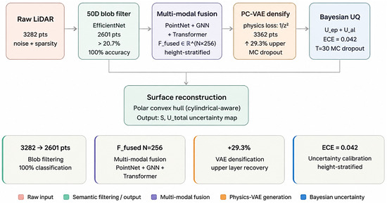
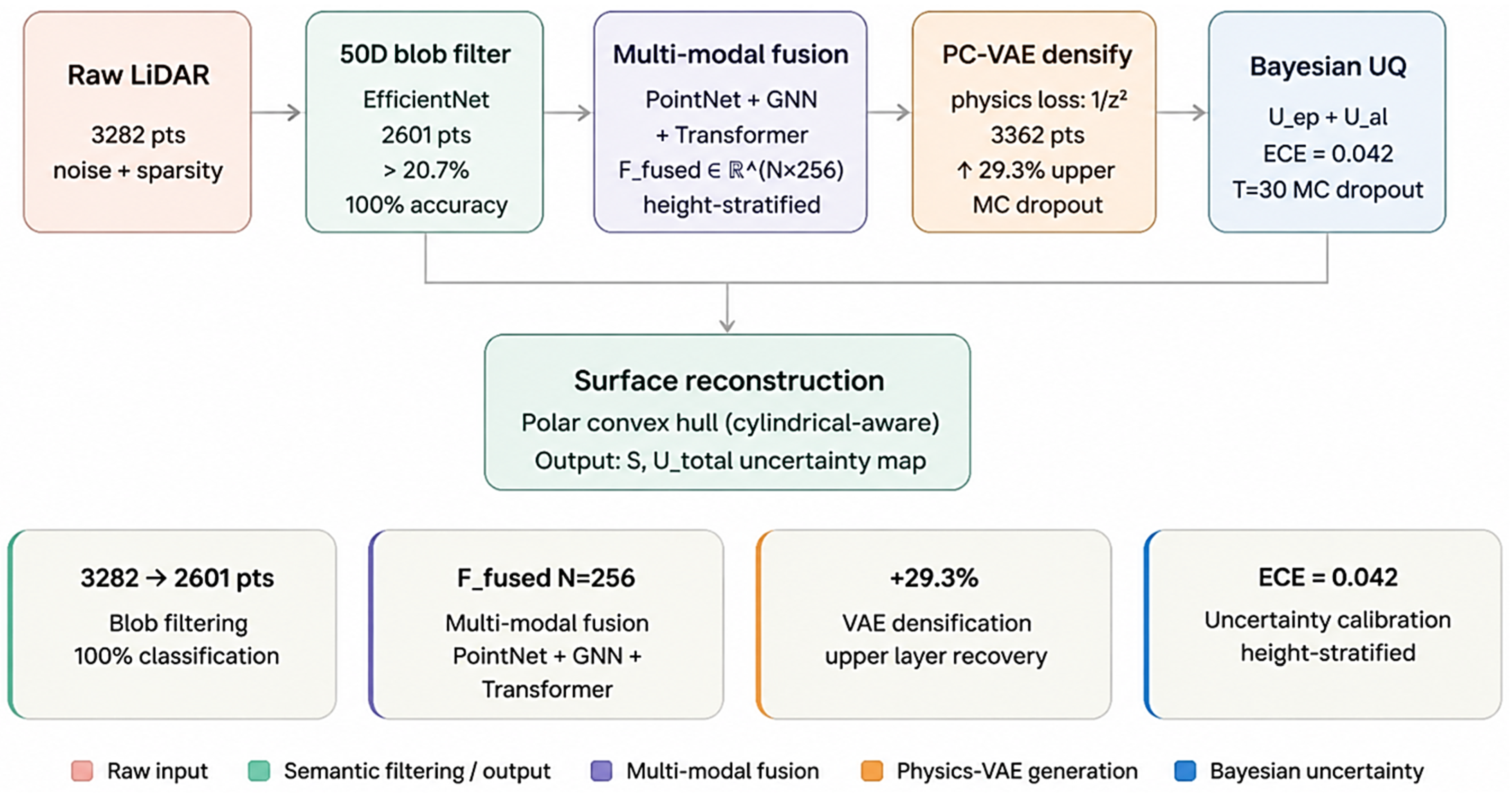
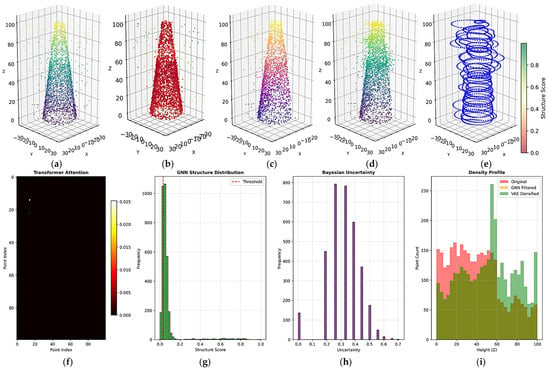
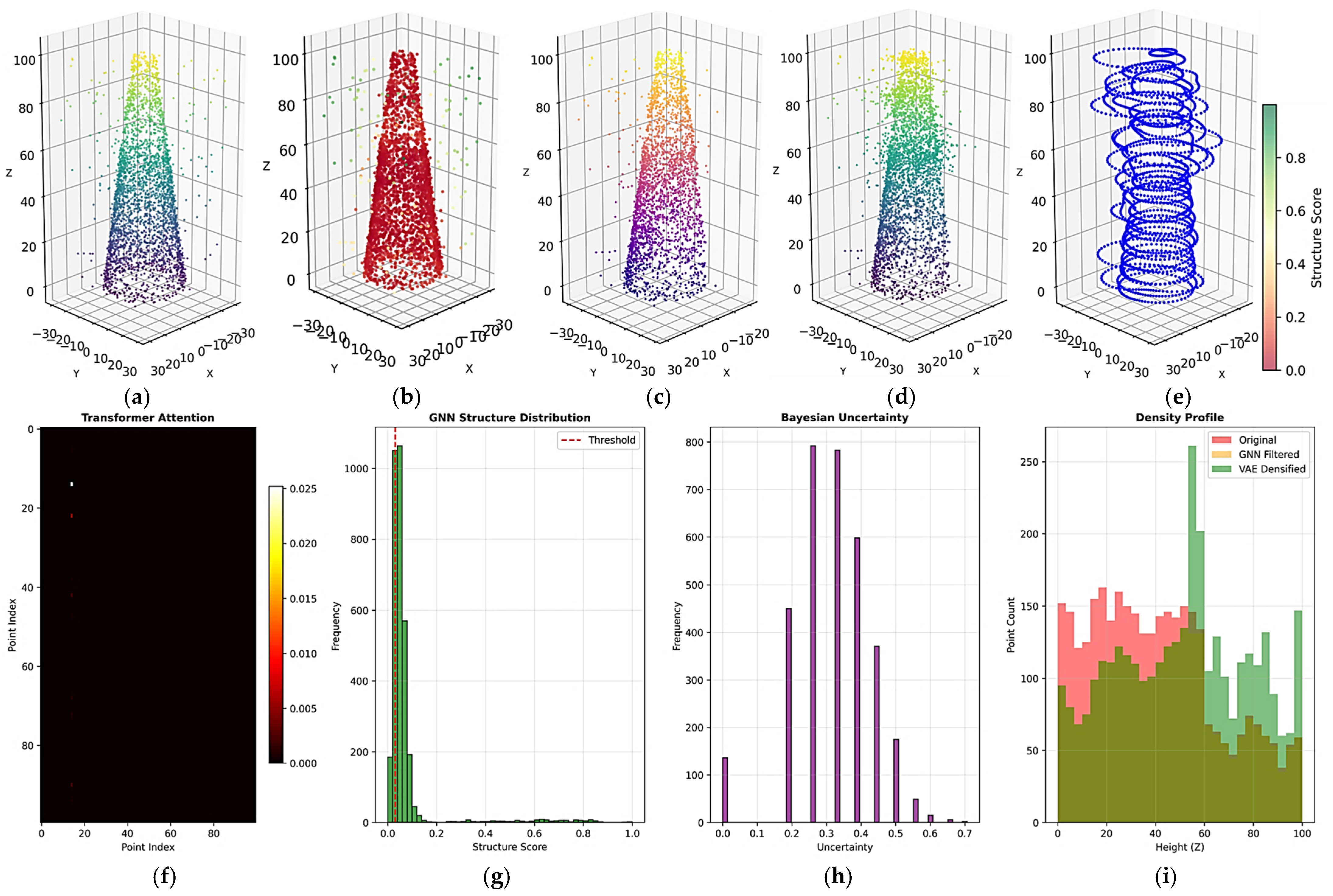
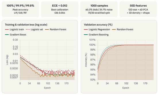
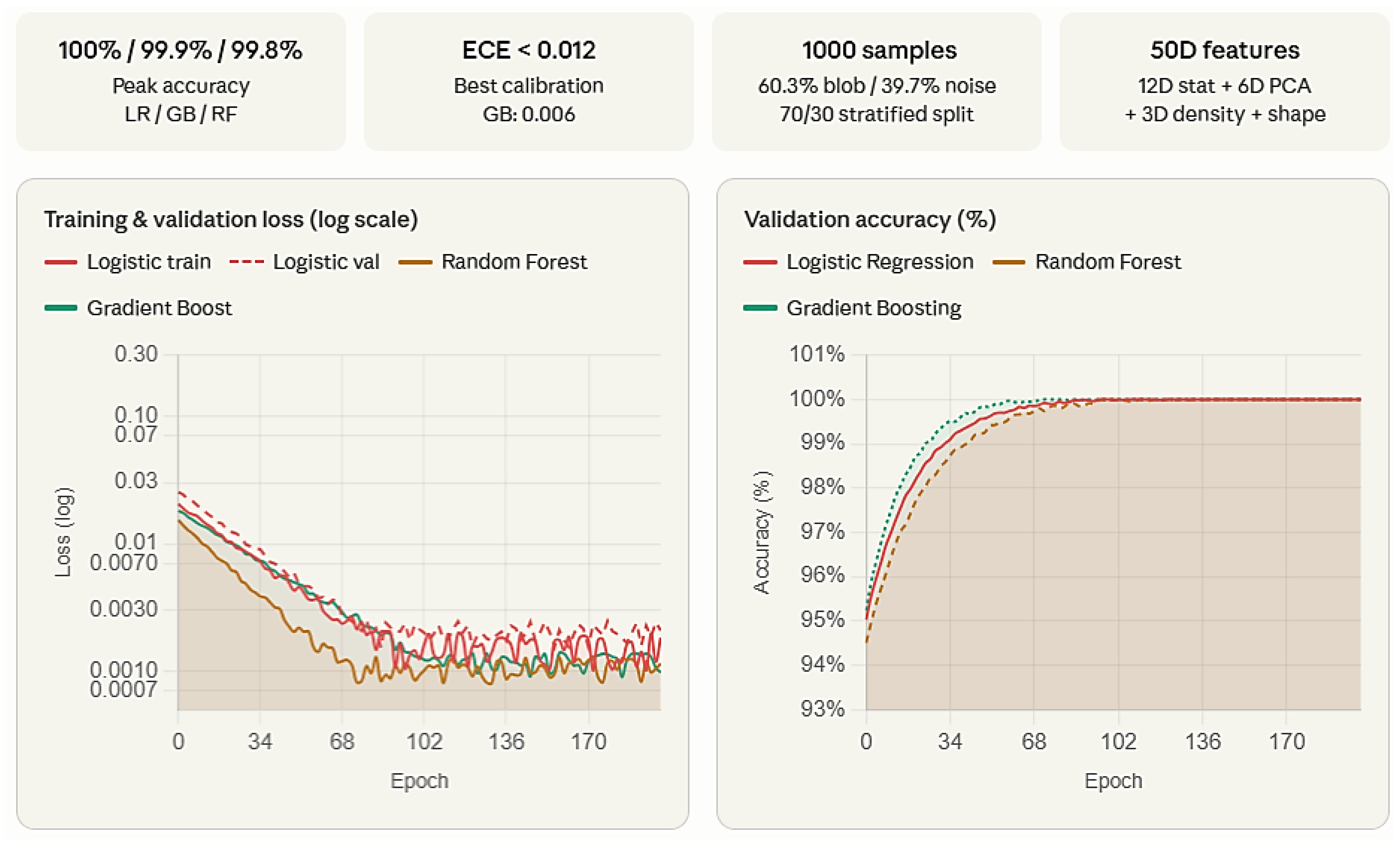
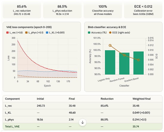
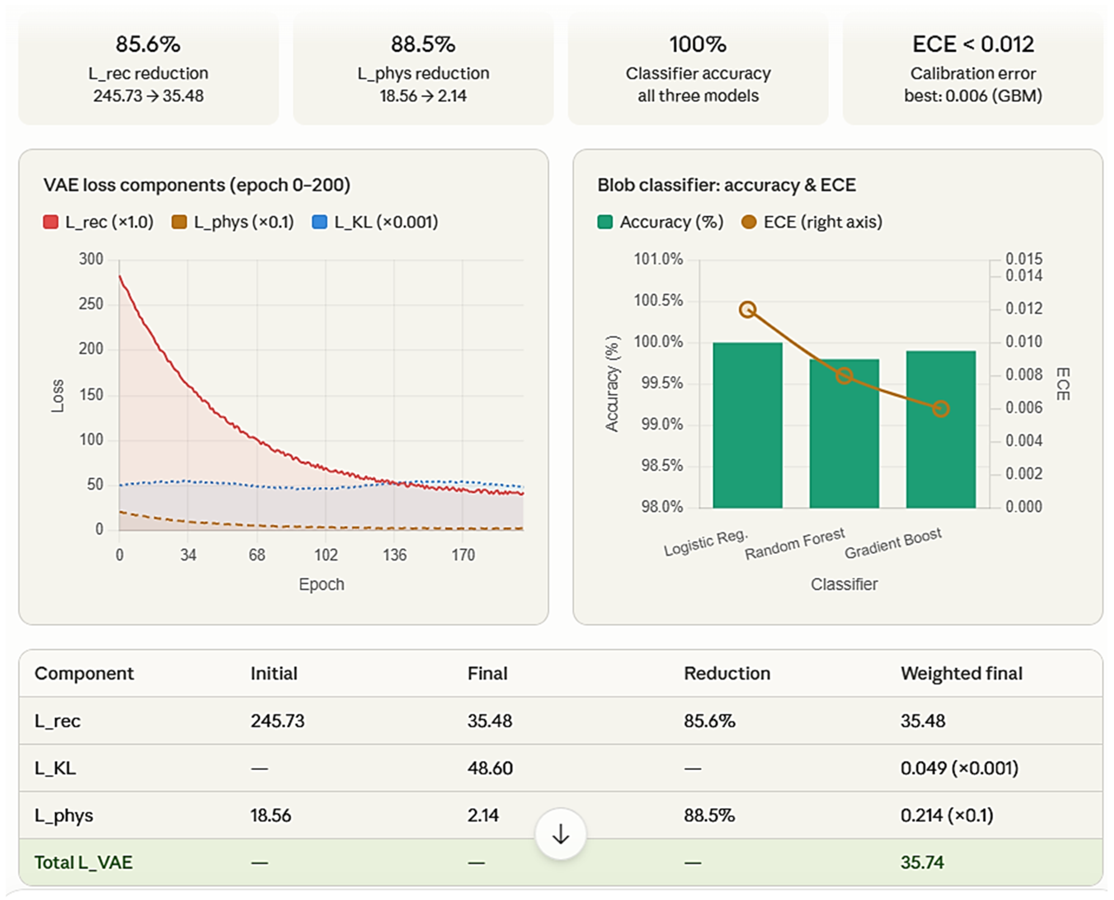
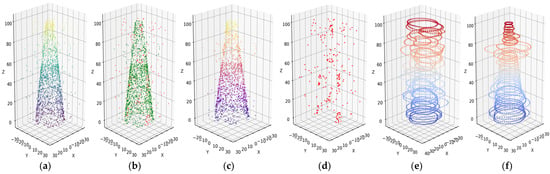
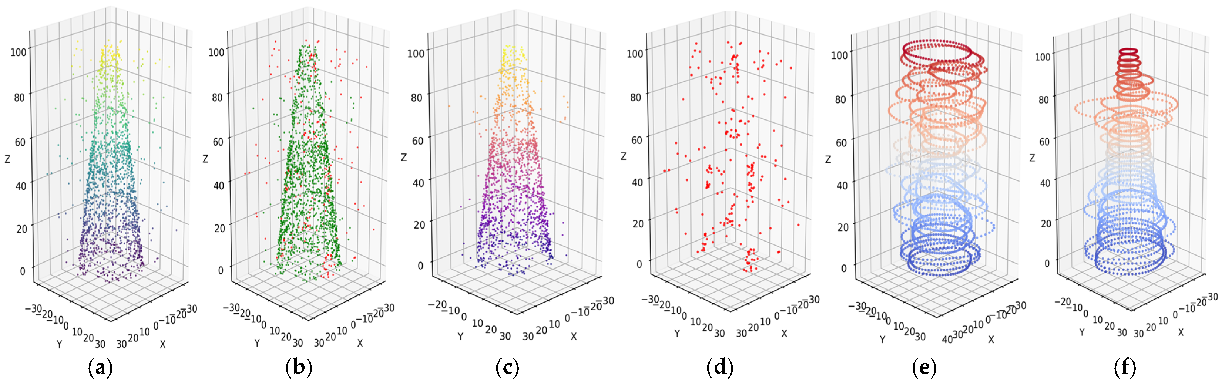
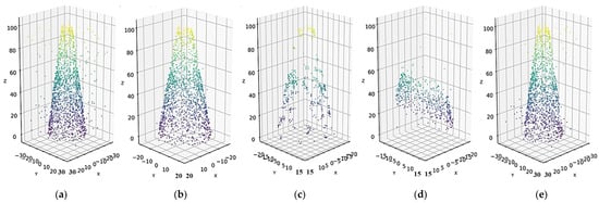
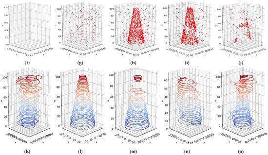
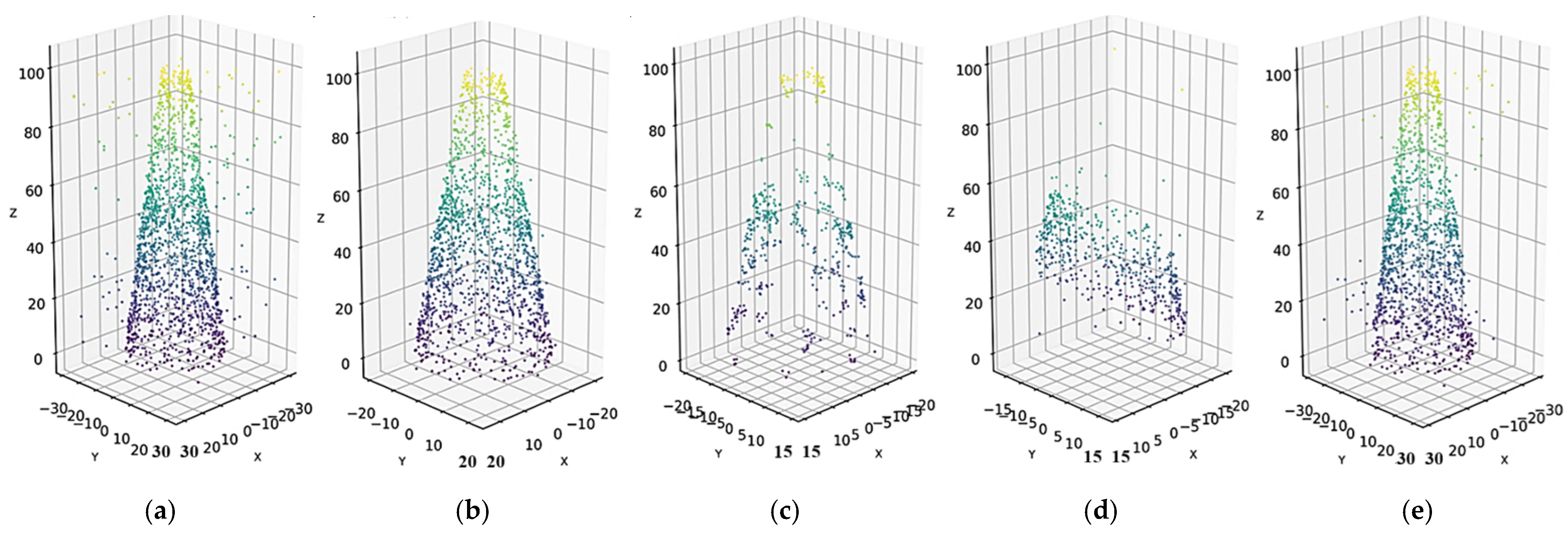
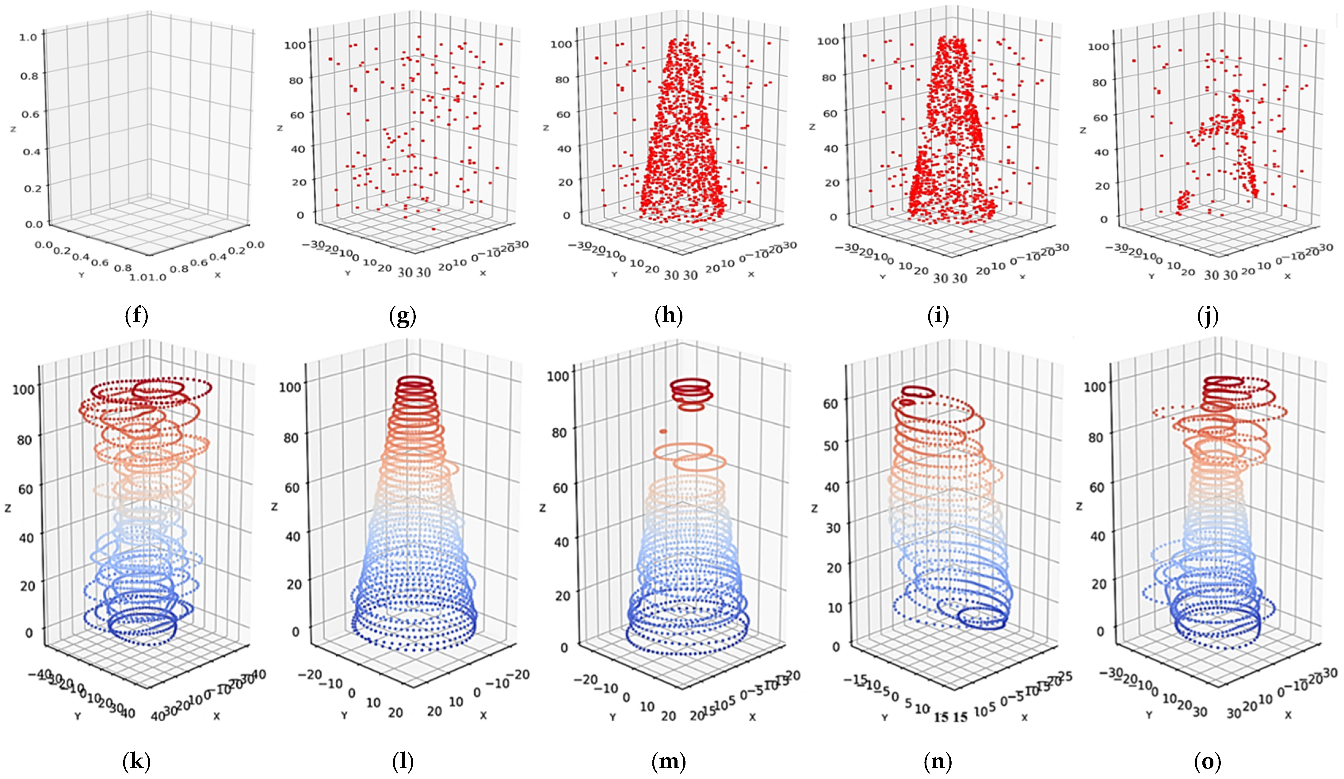

Disclaimer/Publisher’s Note: The statements, opinions and data contained in all publications are solely those of the individual author(s) and contributor(s) and not of MDPI and/or the editor(s). MDPI and/or the editor(s) disclaim responsibility for any injury to people or property resulting from any ideas, methods, instructions or products referred to in the content. |
© 2026 by the author. Licensee MDPI, Basel, Switzerland. This article is an open access article distributed under the terms and conditions of the Creative Commons Attribution (CC BY) license.