A Fault Diagnosis Method for Mobile Communication Networks Based on Improved Convolutional Neural Networks

Abstract

In response to the shortcomings of current mobile communication network (MCN) fault diagnosis methods, such as the insufficient robustness of time-series-spectrum features and the limited ability to capture long-distance dependencies, an improved convolutional neural network is proposed, along with a hybrid diagnosis method based on time-frequency perception and a lightweight deep network (TL-FDN). The TL-FDN introduces a time-series-spectrum feature enhancement module (TFN-E) at the input end, and enhances the robustness of features through a learnable Gabor filter bank. The main architecture employs a hybrid module that integrates a lightweight convolution (LiConv-Block) and a broadcast self-attention (BSA) mechanism (Former-Block), effectively balancing the efficiency of local feature extraction with the capture of global time-series dependencies. Additionally, the model uses a multi-task loss function to achieve joint diagnosis of fault type and fault location. The experimental results show that the average accuracy of the proposed TL-FDN method is 98.6%, which is 3.5% higher than that of the standard convolutional + standard attention baseline method. To strictly evaluate the performance improvement, this paper conducted a non-parametric Wilcoxon signed-rank test in 10 independent experiments. The p-values of the core model indicators were all strictly less than 0.05. These results statistically confirm the superiority of TL-FDN in the fault type identification and location tasks, while maintaining a lightweight parameter quantity suitable for edge-end deployment.

1. Introduction

With the full commercialization of the fifth-generation mobile communication (5G) and the preliminary research on the future 6G network, the mobile communication network is accelerating its evolution towards heterogeneity and densification. However, the sharp increase in network scale and topological complexity has led to an overwhelming number of alarm logs, presenting characteristics such as high concurrency, strong noise, and “alarm storms”, which have made the traditional operation and maintenance mode relying on manual polling and simple rule matching unsustainable [1].

At present, the fault diagnosis of mobile communication networks mainly adopts traditional knowledge-driven methods, focusing on solving the problems of correlation and logical reasoning of alarm data. For the redundant compression of massive alarms, the literature [2] proposed an alarm association rule mining algorithm based on time sliding windows, which improved the traditional Apriori algorithm and effectively extracted frequent fault patterns from historical logs. To cope with the uncertainty brought by the dynamic changes in network topology, the literature [3] applied Bayesian networks to fault diagnosis of complex systems, using data-driven structural learning algorithms to construct fault propagation models and achieve probabilistic reasoning for uncertain faults. Additionally, for the semantic understanding of alarm texts, the literature [4] attempted to build a knowledge graph in the communication field, using entity linking and relationship reasoning to complete the implicit logic between alarms. However, these methods still fundamentally face the “knowledge bottleneck”: the construction of Bayesian networks and knowledge graphs often relies on a large amount of expert prior knowledge or static topology data. In response to the frequent cell expansion, virtual network element migration, and dynamic arrangement of network slices in 5G networks, the manual maintenance of rule libraries lags behind and is difficult to handle unknown and atypical fault patterns, resulting in insufficient generalization ability of the diagnostic system.

In recent years, artificial intelligence technologies represented by deep learning, with their end-to-end feature extraction capabilities, have gradually become the mainstream direction in the field of fault diagnosis. The literature [5] innovatively introduced convolutional neural networks (CNN) into the field of signal processing. By converting one-dimensional time-series signals into two-dimensional feature maps, this method effectively extracted the deep texture features of faults using the weight-sharing mechanism. This approach has also been widely verified in communication signal analysis. Regarding the long-term dependency problem of alarm sequences, the literature [6] proposed the Transformer architecture and its self-attention mechanism (Self-Attention), which completely changed the sequence modeling paradigm. The literature [7] subsequently applied it to industrial fault diagnosis, proving that Transformer outperforms traditional LSTM networks in capturing global temporal correlations. Additionally, for the common problems of label scarcity and long-tail distribution in the current network, the literature [8] proposed a data augmentation and diagnosis framework based on generative adversarial networks (GAN), effectively improving the recognition rate of small-sample faults. Although deep learning models perform well, directly applying them to mobile communication edge-side diagnosis still faces challenges [9]: first, noise sensitivity; base station alarms contain a large amount of non-stationary noise caused by signal flashouts, and standard convolution kernels are difficult to effectively filter out; second, model lightweighting requirements; the existing Transformer or deep CNN parameters are huge and difficult to deploy on edge gateways with limited computing power; third, topological dependence [10,11,12]; existing end-to-end models often ignore the implicit device logical location information (such as SCTP links, radio frequency units) in alarm text, resulting in limited positioning accuracy [13,14,15].

In conclusion, this paper proposes a mobile communication network fault diagnosis method based on a hybrid deep network (TL-FDN). Different from the existing research works that directly adopt a general architecture, the innovation of the TL-FDN method lies in the domain-specific architecture collaboration and adaptation for the edge scenarios of mobile communication networks: (1) An audio-frequency neural feature enhancement module (TFN-E) is introduced, which uses learnable Gabor filter groups to address the basic challenge of non-stationary noise at the source end; (2) The deep separable convolution (LiConv-Blocks) and the efficient broadcast self-attention (BSA) mechanism are adjusted and integrated to form a lightweight “information bottleneck”, balancing local feature extraction and global temporal dependency capture under strict edge deployment constraints. Finally, through a multi-task joint training framework, this model can simultaneously perform real-time fault type diagnosis and logical location diagnosis, thereby establishing a clear boundary between standard lightweight technologies and professional industrial diagnosis requirements [16,17,18].

The rest of this article is structured as follows. Section 2 introduces the related work. Section 3 explains the basic principles of convolutional neural networks. Section 4 details the proposed improved architecture. Section 5 presents the data and feature processing. Section 6 showcases the experiments and analysis. Section 7 summarizes the content of this article.

2. Related Work

In recent years, deep learning has significantly advanced fault diagnosis in Mobile Communication Networks (MCNs). Existing solution methods can generally be categorized into CNN-based approaches, Transformer-based architectures, and multi-task learning frameworks [19].

2.1. Existing Solution Methods and Limitations

Convolutional Neural Networks (CNNs), particularly 1D-CNNs, have been widely adopted to directly process raw 1D sequential signals for fault classification [1]. While these models excel at extracting local receptive features efficiently, they often exhibit high sensitivity to complex background noise and lack the ability to capture comprehensive time-frequency joint representations. On the other hand, to model long-range global dependencies within sequence data, recent studies have increasingly incorporated Transformer architectures and standard self-attention mechanisms. However, the $\mathrm{O}\left({\mathrm{N}}^2\right)$ computational complexity of standard self-attention incurs massive parameter counts and floating-point operations (FLOPs), rendering them highly impractical for deployment on resource-constrained edge devices. Furthermore, while some research has explored Multi-Task Learning (MTL) to predict fault types and locations, these models typically rely on heavy cascaded branches, failing to achieve an optimal balance between feature synergy and a lightweight footprint.

2.2. How the Proposed TL-FDN Improves upon the State-of-the-Art

To overcome these limitations and effectively compete with existing advanced methods, this study proposes the TL-FDN architecture, which incorporates three targeted improvement measures. Firstly, to overcome the noise sensitivity of the direct 1D-CNN, a time-frequency domain enhancement (TFN-E) module with a Gabor filter bank is introduced, which can effectively map the signal to the two-dimensional time-frequency domain before deep extraction. Secondly, to address the computational bottleneck of the standard Transformer, a broadcast self-attention (BSA) mechanism is introduced in the pre-block, significantly reducing the floating-point operation volume while maintaining global context awareness. Finally, these components are integrated into a unified multi-task learning framework, using lightweight convolution (LiConv) blocks, achieving collaborative and highly accurate predictions for fault types and locations, while maintaining extremely low parameter overhead.

To provide a clear overview, Table 1 compares the existing representative solutions with the proposed TL-FDN, highlighting the specific problems solved and the corresponding contributions of this paper.

Table 1. Comparison of the current most advanced methods with the proposed model.

Article/Year	Problem Addressed	Solution Method	Features	Contribution of Our Model
Ref 1, 2025 [20].	Fault diagnosis based on raw 1D signals	One-Dimensional Convolutional Neural Network (1D-CNN)	Extracts features directly from time-domain waveforms efficiently, but typically lacks robustness against complex background noise.	Overcomes noise sensitivity: Employs the TFN-E module with Gabor filter banks to dynamically map 1D signals into robust 2D time-frequency features before deep extraction.
Ref 2, 2026 [21].	Global dependency modeling for fault feature extraction	Transformer architectures/Self-Attention mechanisms	Captures long-range dependencies effectively, but standard self-attention incurs extremely high computational complexity $\left(\mathrm{O}\left({\mathrm{N}}^2\right)\right).$	Improves edge-efficiency: Replaces standard self-attention with Broadcast Self-Attention (BSA), drastically reducing parameter counts and FLOPs while maintaining global contextual awareness.
Ref 3, 2025 [22].	Fault Detection, Classification, and Localization	Multi-Task Learning (MTL) framework with attention	Performs joint tasks effectively but relies on complex network branches, which can be computationally heavy for edge gateways.	Enhances feature synergy and efficiency: Proposes a highly unified Multi-task Learning architecture ($\mathsf{\lambda }$= 0.5) combined with lightweight LiConv Blocks, achieving high accuracy with minimal parameters.
Rebuild the convolutional neural network	Edge-side mobile communication network fault diagnosis	TFN-E + LiConv Blocks + Former-Block (BSA)	Real-time, lightweight, noise-resistant, and high accuracy for multi-task scenarios.	Comprehensive Solution: Achieves an optimal trade-off between multi-task diagnostic accuracy and computational efficiency for edge-side deployment.

3. Principles of Convolutional Neural Networks

Convolutional Neural Networks (CNN) are one of the most effective intelligent algorithms in the field of deep learning for grid-like topological data such as images and time series signals. The core design concept of CNN lies in the use of local connectivity and weight sharing mechanisms, which enable it to automatically extract hierarchical and translation-invariant features from the input data efficiently, significantly reducing the number of model parameters and making it a powerful tool for fault diagnosis of time series signals. The classic structure of CNN usually consists of convolutional layers, pooling layers, and fully connected layers. Each layer is connected through nonlinear activation functions, jointly constructing the deep feature abstraction ability.

After the MCN alarm data is preprocessed, it is usually transformed into a multi-dimensional time series matrix X as the input of the model. This input matrix X precisely represents the distribution of the characteristics of M alarm types over L time steps in a sequence, and its mathematical expression is given by Equation (1):

$$\mathit{X}={\left[{\mathit{x}}_1,{\mathit{x}}_2,\cdots ,{\mathit{x}}_t,\cdots ,{\mathit{x}}_L\right]}^T\in {\mathit{R}}^{L\times M},$$

(1)

In the formula, X is the input feature matrix, M represents the feature dimension (for example, the number of alarm types), and L is the length of the time series sequence (the size of the time window). $x_t\in {\mathit{R}}^M$ denotes the feature vector at time t. The convolution layer is the core feature extraction unit of CNN. Its function is to obtain a set of optimal convolution kernels W through training, thereby automatically capturing the local patterns of the input time series data. The convolution operation is to perform a sequence convolution operation mapping on the input sequence data X and the convolution kernel ${\mathit{W}}_c^j$, strictly following the principles of local connection and weight sharing. For one-dimensional time series convolution, the calculation expression on the c-th layer and the j-th feature map is defined in Equation (2):

$${\mathit{a}}_c^j\left[i\right]=f_r\left({\displaystyle {\sum }_{m=1}^M}{\displaystyle {\sum }_{k=1}^K}\mathit{X}\left[i+k-1,m\right]\cdot {\mathit{W}}_c^j\left[k,m\right]+b_c^j\right),$$

(2)

In the formula, ${\mathit{W}}_c^j\in R^{K\times M}$ represents the j-th convolution kernel, with the dimension K being the width of the local time window, usually $K\ll L$, which determines the range of local dependencies that the model can capture; $b_c^j$ is the corresponding bias term, used to adjust the starting point of the activation function output; $a_c^j$ is the j-th output feature map generated by ${\mathit{W}}_c^j$; $f_r\left(\cdot \right)$ represents the nonlinear activation function. Typically, the ReLU function $f_r\left(\mathrm{z}\right)=\mathrm{m}\mathrm{a}\mathrm{x}\left(\mathrm{z},0\right)$ is used, which is widely applied in deep networks due to its simple calculation, non-saturating characteristic, and ability to alleviate the problem of gradient dispersion, enabling the network to handle nonlinear relationships.

The pooling layer follows the convolution layer and mainly reduces the temporal dimension of the feature information output by the convolution layer through downsampling operations. This process is an important means for CNN to reduce the number of parameters and computational cost, while enhancing the model’s robustness to small feature deformations (such as time drift and phase shift). The expression of the pooling operation pool() concisely summarizes the process of information compression as shown in Equation (3):

$${\mathit{a}}_p^j=\mathrm{p}\mathrm{o}\mathrm{o}\mathrm{l}\left({\mathit{a}}_c^j\right) ,$$

(3)

The fully connected layer is located at the end of the CNN structure, responsible for the final recombination and mapping of the high-level abstract features obtained after multiple convolutions and pooling, and for performing the final classification task. The feature vector $a_{\mathrm{f}\mathrm{l}\mathrm{a}\mathrm{t}\mathrm{t}\mathrm{e}\mathrm{n}}$ after the global pooling or flattening operation is input into the fully connected layer, and its calculation expression reflects the linear transformation from the feature space to the decision space, as expressed in Equation (4):

$$\mathit{z}={\mathit{W}}_{\mathrm{f}\mathrm{c}}{\mathit{a}}_{\mathrm{f}\mathrm{l}\mathrm{a}\mathrm{t}\mathrm{t}\mathrm{e}\mathrm{n}}+{\mathit{b}}_{\mathrm{f}\mathrm{c}},$$

(4)

The final output layer maps the features into the probability distribution $\widehat{y}:$ for each fault category through the Softmax activation function, as shown in Equation (5):

$${\widehat{\mathit{y}}}_c={\displaystyle \frac{e^{{\mathbf{z}}_c}}{{\displaystyle {\sum }_{j=1}^C}{e}^{{\mathbf{z}}_j}}},$$

(5)

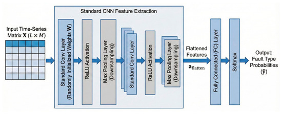
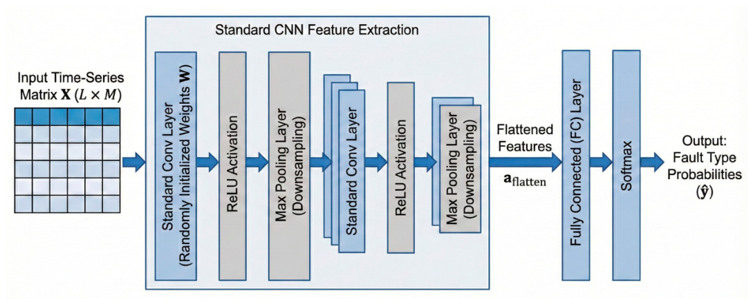
Here, C represents the total number of categories. This indicates that the original design intention of the conventional CNN architecture is usually for a single classification task, and its output merely represents the probability distribution of the samples belonging to a specific fault type, as illustrated in Figure 1.

Figure 1. Improvement of the convolutional neural network structure.

4. Improvement of Convolutional Neural Network Principles

4.1. Improvement for Feature Robustness: Time-Frequency-Neural Feature Enhancement Module (TFN-E)

In response to the essential deficiencies of traditional CNNs in MCN fault diagnosis, such as insufficient feature robustness, limited capture of long-distance dependencies, and single-output tasks as detailed in Section 1, this paper proposes the TL-FDN hybrid diagnosis method based on the traditional CNN architecture. TL-FDN achieves a deep structural reconstruction and functional enhancement of the CNN structure by introducing three innovative modules and a multi-task learning framework.

To overcome the generalization constraints of traditional CNN convolution kernels and enhance the resistance of features to environmental noise and non-stationary fluctuations from the source, TL-FDN constructs a time-frequency feature enhancement module (TFN-E) in the first step of feature extraction. The core innovation of this module lies in parameterizing the unconstrained convolution kernels of traditional CNNs as learnable Gabor filter banks.

The Gabor filter is regarded as an ideal tool for signal analysis due to its optimal localization characteristics in both the time domain and the frequency domain (i.e., satisfying the minimum bound of the Heisenberg uncertainty principle). It can simulate the perception mechanism of the human visual system for specific frequency and direction textures. In TFN-E, each convolution kernel $K_{\mathrm{T}\mathrm{F}\mathrm{N}-\mathrm{E}}$ is forcibly constrained to the form of a Gabor function, and its key parameters are no longer the randomly initialized weight matrix, but the center frequency $f_c$ and scale parameter ${\sigma }_{\mathrm{c}}$ with clear physical meanings. These parameters, as trainable parameters in the network, are integrated into the optimization process of backpropagation. This design enables the filter to adaptively adjust its passband range according to the statistical characteristics of MCN alarm data, thereby optimally capturing the frequency components that best distinguish faults while suppressing noise outside the frequency band.

The mathematical analytical form of the Gabor filter, that is, the constraint function of the TFN-E convolution kernel, is defined in Equation (6):

$$G\left(t;f,\sigma \right)=e^{-\pi {\displaystyle \frac{t^2}{{\sigma }^2}}}\cdot e^{j2\pi ft},$$

(6)

In practical applications, the real part of the kernel is usually used. The calculation of the output $F_{\mathrm{e}\mathrm{n}\mathrm{h}}$ of the TFN-E layer follows the convolution form, but its convolution kernel $K_{\mathrm{T}\mathrm{F}\mathrm{N}-\mathrm{E}}$ is constrained by the Gabor function, as shown in Equation (7):

$$F_{\mathrm{e}\mathrm{n}\mathrm{h}}=\mathrm{R}\mathrm{e}\mathrm{L}\mathrm{U}\left(\mathit{X}\ast \mathrm{R}\mathrm{e}\left(G\left(t;f,\sigma \right)\right)+b\right),$$

(7)

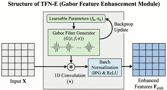
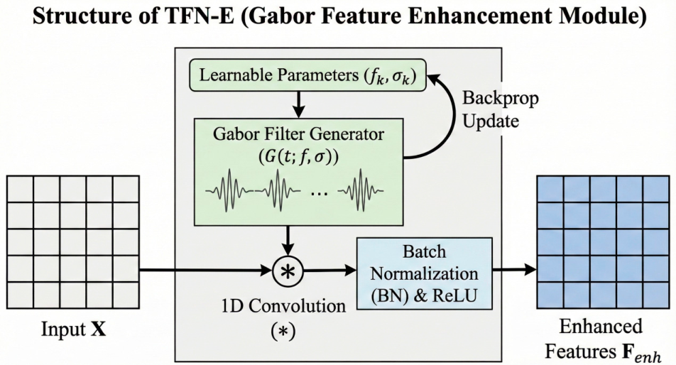
The $F_{\mathrm{e}\mathrm{n}\mathrm{h}}$ output at this layer possesses a highly powerful adaptive time-frequency filtering capability. It can dynamically enhance the key frequency components of the fault signal, effectively suppress non-key noise and background fluctuations, thereby fundamentally improving the robustness and discrimination of the input features, as depicted in Figure 2.

Figure 2. Gabor filter structure.

4.2. Improvement in Computational Efficiency: Lightweight Local Feature Extraction Core (LiConv-Block)

Inspired by the success of Deep Separable Convolution (DSC) in lightweight visual models [23], the DSC operation was applied to the LiConv-Block in this paper to clearly separate the temporal and channel feature extraction of multi-channel network alerts.

Traditional CNN relies on standard convolutional layers for feature extraction. The parameter quantity $P_{\mathrm{s}\mathrm{t}\mathrm{d}}=C_{\mathrm{i}\mathrm{n}}\times K\times C_{\mathrm{o}\mathrm{u}\mathrm{t}}$ increases linearly with the number of channels and the size of the convolution kernel. This not only increases the training burden but also severely hinders the deployment of the model on edge nodes of MCN with limited computing resources. To meet the lightweight requirements, TL-FDN adopts depthwise separable convolution (Depthwise Separable Convolution, DSC) to construct LiConv-Block, fundamentally optimizing the computational efficiency of the feature extraction layer of CNN.

DSC rigorously decomposes the standard convolution operation into two independent and computationally less costly steps: 1. Depthwise Convolution: Performs a local convolution of $K\times 1$ on each input channel independently, without mixing channels. Its purpose is to extract spatial/temporal features of each channel. The parameter quantity is $P_{\mathrm{d}\mathrm{e}\mathrm{p}\mathrm{t}\mathrm{h}}=C_{\mathrm{i}\mathrm{n}}\times K.$ 2. Pointwise Convolution: Uses a $1\times 1$ convolution kernel to linearly combine all the outputs of the depthwise convolution, achieving information aggregation and feature fusion across channels. The parameter quantity is $P_{\mathrm{p}\mathrm{o}\mathrm{i}\mathrm{n}\mathrm{t}}=C_{\mathrm{i}\mathrm{n}}\times C_{\mathrm{o}\mathrm{u}\mathrm{t}}$.

The total parameter quantity $P_{\mathrm{D}\mathrm{S}\mathrm{C}}$ of the DSC has been significantly reduced, and the computational complexity has also decreased substantially. The formula for comparing the parameter quantities is calculated using Equation (8):

$${\displaystyle \frac{P_{\mathrm{D}\mathrm{S}\mathrm{C}}}{P_{\mathrm{s}\mathrm{t}\mathrm{d}}}}={\displaystyle \frac{C_{\mathrm{i}\mathrm{n}}\times K+C_{\mathrm{i}\mathrm{n}}\times C_{\mathrm{o}\mathrm{u}\mathrm{t}}}{C_{\mathrm{i}\mathrm{n}}\times K\times C_{\mathrm{o}\mathrm{u}\mathrm{t}}}}={\displaystyle \frac{1}{C_{\mathrm{o}\mathrm{u}\mathrm{t}}}}+{\displaystyle \frac{1}{K}},$$

(8)

When the number of output channels $C_{\mathrm{o}\mathrm{u}\mathrm{t}}$ is large, this ratio approaches $1/K$, achieving significant parameter compression. The LiConv-Block is composed of DSC, batch normalization (Batch Normalization, BN) layers, and ReLU activation functions. By stacking such modules, it optimizes the model parameters and computational cost while ensuring the local feature extraction capability, achieving an efficient improvement of the CNN local feature extraction module.

4.3. Improvement for Long-Distance Dependency: Integration of an Efficient Global Dependency Modeling Mechanism (Former-Block)

To address the $O\left(N^2\right)$ complexity issue in the standard Transformer, this paper adopts the broadcast self-attention (BSA) mode [6]. In our architecture, the previous block acts as a global feature aggregator, specifically designed to handle the robust local representations generated by the previous LiConv-blocks.

Traditional CNNs can only indirectly expand the receptive field through multiple convolutions and pooling operations, and have extremely low efficiency in capturing long-distance dependencies across long time windows. This makes it difficult for the model to understand the entire process of MCN failure evolution. TL-FDN, after the LiConv-Block, innovatively introduces a Former-Block based on the Transformer architecture, and uses the broadcast self-attention (BSA) mechanism to achieve efficient global dependency modeling.

The standard self-attention mechanism calculates the similarity matrix between all position pairs, and its computational complexity is proportional to the square of the sequence length L, i.e., $O\left(L^2\right)$. When dealing with long sequence MCN data, this will impose a huge computational and memory burden. The BSA mechanism has optimized this bottleneck by employing ingenious matrix decomposition and broadcast operations, avoiding the complete calculation of the $Q\cdot K^T$ matrix, and successfully reducing the complexity to approximately linear complexity $O\left(L\right)$. The BSA mechanism first generates a global context vector, and then “broadcasts” it to each position of the sequence, thereby achieving the interaction of global information. Its core calculation process can be expressed as Equation (9):

$$A=\mathrm{Softmax}\left({\displaystyle \frac{Q\cdot K_{\mathrm{global}}^T}{\sqrt{d_k}}}\right), F_{\mathrm{BSA}}=A\cdot V_{\mathrm{global}}+\mathrm{Residue},$$

(9)

This improvement enables TL-FDN to capture the global temporal correlations within L time windows with extremely high computational efficiency, resolving the bottleneck problem of traditional CNNs in long sequence modeling. The final output of the former block, the feature vector $F_{\mathrm{f}\mathrm{i}\mathrm{n}\mathrm{a}\mathrm{l}}$, integrates robust local features and key global dependencies, achieving a functional enhancement of the traditional CNN architecture.

4.4. Improvement for Output Singularity: Multi-Task Joint Diagnosis Mechanism

In response to the limitation of conventional CNNs that can only output a single classification result, TL-FDN has structurally expanded the output layer and designed a dual-branch fully connected layer, which is respectively used for fault type identification and fault location determination. This improvement is based on the multi-task learning (Multi-Task Learning, MTL) concept. By sharing the underlying feature extraction network (TFN-E, LiConvBlock, Former-Block), the model can learn general feature representations that are discriminative for both tasks. The fault location information can serve as an implicit “spatial constraint” to assist the model in more accurately determining the fault type; conversely, the semantic information of the fault type also helps to rule out impossible fault locations. The model uses the joint loss function $L_{\mathrm{t}\mathrm{o}\mathrm{t}\mathrm{a}\mathrm{l}}$ for end-to-end optimization training, as defined in Equation (10):

$$L_{\mathrm{t}\mathrm{o}\mathrm{t}\mathrm{a}\mathrm{l}}=L_{\mathrm{t}\mathrm{y}\mathrm{p}\mathrm{e}}+\lambda L_{\mathrm{l}\mathrm{o}\mathrm{c}\mathrm{a}\mathrm{t}\mathrm{i}\mathrm{o}\mathrm{n}},$$

(10)

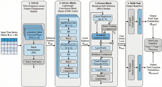
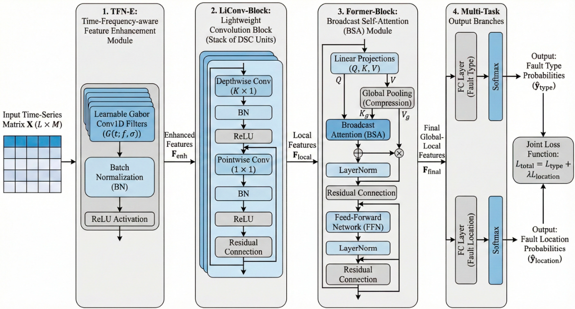
Here, $L_{\mathrm{t}\mathrm{y}\mathrm{p}\mathrm{e}}$ and $L_{\mathrm{l}\mathrm{o}\mathrm{c}\mathrm{a}\mathrm{t}\mathrm{i}\mathrm{o}\mathrm{n}}$ represent the cross-entropy losses of the two tasks, and λ is the balancing factor. The complete architecture of the proposed TL-FDN is presented in Figure 3.

Figure 3. Improved convolutional neural network structure.

As shown in Figure 3, the structure of the proposed model consists of four consecutive stages. Firstly, the TFN-E module serves as the front end, using learnable Gabor 1D filters to convert the original time series matrix into a robust time-frequency representation. Subsequently, the LiConv-Block (Stage 2) is composed of stacked depthwise separable convolutional units, which are used to efficiently extract local temporal patterns from the enhanced features. To overcome the limitations of local receptive fields, the Former-Block (Stage 3) integrates the broadcast self-attention (BSA) mechanism to capture the global topological dependencies between alarms. Finally, the fused global-local features are sent to the multi-task output branch (Stage 4), which simultaneously maps these representations to precisely predict the specific fault type and location.

4.5. Overall Algorithm Flow and Pseudo-Code

To clearly illustrate the execution logic of the proposed method, Algorithm 1 presents the detailed training process of the model. The explicit inputs to the algorithm include the preprocessed multidimensional time-series training dataset ${\mathcal{D}}_{\mathrm{t}\mathrm{r}\mathrm{a}\mathrm{i}\mathrm{n}}$ the validation set ${\mathcal{D}}_{\mathrm{v}\mathrm{a}\mathrm{l}}$, and essential hyperparameters. During the forward propagation phase (Lines 5–10), the raw input of each mini-batch ($X_{\mathrm{b}\mathrm{a}\mathrm{t}\mathrm{c}\mathrm{h}}$) first passes through the TFN-E module, where learnable Gabor filters dynamically extract robust time-frequency features. Subsequently, the LiConv-Block efficiently extracts local temporal features with minimal parameter overhead, which are then fed into the Former-Block to capture global sequence dependencies via the broadcast self-attention (BSA) mechanism. Finally, the network splits into two fully connected branches to output the probability distributions for the fault type and location. During the backward propagation phase (Lines 12–17), the cross-entropy losses for both multi-task objectives are calculated against the ground truth labels, and a joint loss function ${\mathrm{L}}_{\mathrm{t}\mathrm{o}\mathrm{t}\mathrm{a}\mathrm{l}}$ is computed. The gradients are derived, and the shared underlying parameters $\Theta$ are updated simultaneously using the AdamW optimizer. To ensure training stability and prevent overfitting, a dynamic learning rate decay mechanism is integrated at the end of each epoch, which halves the learning rate $\eta$ if the validation loss plateaus (Lines 20–24).

Algorithm 1: Training Process

Require: Training set ${\mathcal{D}}_{\mathrm{t}\mathrm{r}\mathrm{a}\mathrm{i}\mathrm{n}}=\{\left(X^{\left(i\right)},y_{\mathrm{t}\mathrm{y}\mathrm{p}\mathrm{e}}^{\left(i\right)},y_{\mathrm{l}\mathrm{o}\mathrm{c}}^{\left(i\right)}\right){\}}_{i=1}^N;$ Validation set ${\mathcal{D}}_{\mathrm{v}\mathrm{a}\mathrm{l}};$ Max epochs $E;$ Batch size $B;$ Initial learning rate $\eta ;$ Balance factor $\lambda .$  Ensure: Optimized model parameters $\Theta .$ 1: Initialize model parameters $\Theta$ randomly 2: for $epoch=1$ to $E$ do 3: Shuffle the training dataset ${\mathcal{D}}_{\mathrm{t}\mathrm{r}\mathrm{a}\mathrm{i}\mathrm{n}}$ 4:  for each mini-batch $\left(X_{\mathrm{b}\mathrm{a}\mathrm{t}\mathrm{c}\mathrm{h}},Y_{\mathrm{t}\mathrm{y}\mathrm{p}\mathrm{e}},Y_{\mathrm{l}\mathrm{o}\mathrm{c}}\right)\in {\mathcal{D}}_{\mathrm{t}\mathrm{r}\mathrm{a}\mathrm{i}\mathrm{n}}$ of size $B$ do 5:  $⊳$ Forward Propagation Phase 6:  $F_{\mathrm{e}\mathrm{n}\mathrm{h}}\leftarrow \mathrm{R}\mathrm{e}\mathrm{L}\mathrm{U}\left(X_{\mathrm{b}\mathrm{a}\mathrm{t}\mathrm{c}\mathrm{h}}⊛\mathrm{R}\mathrm{e}\left(G\left(t;f,\sigma \right)\right)+{\mathrm{b}}_{\mathrm{T}\mathrm{F}\mathrm{N}}\right)$ 7:  $F_{\mathrm{l}\mathrm{o}\mathrm{c}\mathrm{a}\mathrm{l}}\leftarrow \mathrm{L}\mathrm{i}\mathrm{C}\mathrm{o}\mathrm{n}\mathrm{v}\mathrm{B}\mathrm{l}\mathrm{o}\mathrm{c}\mathrm{k}\left(F_{\mathrm{e}\mathrm{n}\mathrm{h}},{\Theta }_{\mathrm{L}\mathrm{i}\mathrm{C}\mathrm{o}\mathrm{n}\mathrm{v}}\right)$ 8:  $F_{\mathrm{f}\mathrm{i}\mathrm{n}\mathrm{a}\mathrm{l}}\leftarrow \mathrm{F}\mathrm{o}\mathrm{r}\mathrm{m}\mathrm{e}\mathrm{r}\mathrm{B}\mathrm{l}\mathrm{o}\mathrm{c}\mathrm{k}\left(F_{\mathrm{l}\mathrm{o}\mathrm{c}\mathrm{a}\mathrm{l}},{\Theta }_{\mathrm{F}\mathrm{o}\mathrm{r}\mathrm{m}\mathrm{e}\mathrm{r}}\right)$ 9:  ${\widehat{Y}}_{\mathrm{t}\mathrm{y}\mathrm{p}\mathrm{e}}\leftarrow \mathrm{S}\mathrm{o}\mathrm{f}\mathrm{t}\mathrm{m}\mathrm{a}\mathrm{x}\left({\mathrm{F}\mathrm{C}}_{\mathrm{t}\mathrm{y}\mathrm{p}\mathrm{e}}\left(F_{\mathrm{f}\mathrm{i}\mathrm{n}\mathrm{a}\mathrm{l}},{\Theta }_{\mathrm{F}\mathrm{C}1}\right)\right)$ 10:   ${\widehat{Y}}_{\mathrm{l}\mathrm{o}\mathrm{c}}\leftarrow \mathrm{S}\mathrm{o}\mathrm{f}\mathrm{t}\mathrm{m}\mathrm{a}\mathrm{x}\left({\mathrm{F}\mathrm{C}}_{\mathrm{l}\mathrm{o}\mathrm{c}}\left(F_{\mathrm{f}\mathrm{i}\mathrm{n}\mathrm{a}\mathrm{l}},{\Theta }_{\mathrm{F}\mathrm{C}2}\right)\right)$ 11: 12:   $⊳$ Loss Calculation and Backpropagation Phase 13:   $L_{\mathrm{t}\mathrm{y}\mathrm{p}\mathrm{e}}\leftarrow \mathrm{CrossEntropy}\left({\widehat{Y}}_{\mathrm{t}\mathrm{y}\mathrm{p}\mathrm{e}},Y_{\mathrm{t}\mathrm{y}\mathrm{p}\mathrm{e}}\right)$ 14:   $L_{\mathrm{l}\mathrm{o}\mathrm{c}}\leftarrow \mathrm{CrossEntropy}\left({\widehat{Y}}_{\mathrm{l}\mathrm{o}\mathrm{c}},Y_{\mathrm{l}\mathrm{o}\mathrm{c}}\right)$ 15:   $L_{\mathrm{t}\mathrm{o}\mathrm{t}\mathrm{a}\mathrm{l}}\leftarrow L_{\mathrm{t}\mathrm{y}\mathrm{p}\mathrm{e}}+\lambda L_{\mathrm{l}\mathrm{o}\mathrm{c}}$ 16:   ${\nabla }_{\Theta }{L}_{\mathrm{t}\mathrm{o}\mathrm{t}\mathrm{a}\mathrm{l}}\leftarrow \mathrm{ComputeGradients}\left(L_{\mathrm{t}\mathrm{o}\mathrm{t}\mathrm{a}\mathrm{l}},\Theta \right)$ 17:   $\Theta \leftarrow \mathrm{A}\mathrm{d}\mathrm{a}\mathrm{m}\mathrm{W}\left(\Theta ,{\nabla }_{\Theta }{L}_{\mathrm{t}\mathrm{o}\mathrm{t}\mathrm{a}\mathrm{l}},\eta \right)$ 18: end for 19: 20:   $⊳$ Dynamic Learning Rate Decay 21:   Evaluate model on validation set ${\mathcal{D}}_{\mathrm{v}\mathrm{a}\mathrm{l}}$ 22:   if validation loss plateaus then 23:     $\eta \leftarrow \eta \times 0.5$ 24:  end if 25: end for 26: return $\Theta$

5. Data Preprocessing and High-Dimensional Feature Construction

The fault diagnosis of MCN relies on the mining and analysis of massive alarm logs. The original alarm data usually exhibit the characteristics of being discrete, unbalanced, containing noise and having a large amount of redundant information. In order for the model to effectively learn the fault patterns, the alarm data must undergo strict preprocessing, time synchronization and high-dimensional feature encoding operations.

5.1. Data Cleaning, Time Synchronization and Multi-Task Label Extraction

The first step in the preprocessing of alarm data is data cleaning and deduplication. This process aims to improve data quality and eliminate the interference of dirty data on model training. Firstly, incomplete records (such as those lacking key fields) caused by transmission errors or system anomalies are eliminated; secondly, the same alarm reported repeatedly within a short period of time is compressed and deduplicated based on a sliding time window; finally, the naming conventions of alarm names for different devices are unified, and a standardized alarm dictionary is established to eliminate heterogeneity. The key fields after cleaning include alarm titles, alarm levels, occurrence times, and involved device IDs, etc.

Next, the time synchronization of the alarm information is carried out. Since alarms are asynchronous, discrete events that occur independently, they cannot be directly used as input for deep learning models. This paper adopts the sliding time window method to convert the discrete events into a continuous time series. A fixed time window length $\mathsf{\Delta }\mathrm{t}=10$ min is set, and the sequence length $\mathrm{L}=12$ is also set, meaning that each sample X covers $\mathrm{L}\times \mathsf{\Delta }\mathrm{t}=120$ min (2 h) of historical information. This multi-time-step sequence design provides sufficient time for the model to capture long-term temporal dependencies.

At the same time, during this stage, the extraction and encoding of multi-task labels are completed. Two classification results, namely the fault type ${\mathrm{Y}}_{\mathrm{t}\mathrm{y}\mathrm{p}\mathrm{e}}$ and the fault location ${\mathrm{Y}}_{\mathrm{l}\mathrm{o}\mathrm{c}\mathrm{a}\mathrm{t}\mathrm{i}\mathrm{o}\mathrm{n}}$, need to be output simultaneously.

Fault type label ${\mathrm{Y}}_{\mathrm{t}\mathrm{y}\mathrm{p}\mathrm{e}}$: Based on MCN fault tree analysis and historical alarm clustering results, hundreds of thousands of fine-grained alarms are mapped and aggregated into $\mathrm{T}=8$ macroscopic fault categories with clear physical meanings (such as: power system failure, transmission link interruption, optical module failure, software logic error, congestion flow control, normal state). The specific mapping between fault categories and their corresponding one-hot encodings is summarized in Table 2.

Table 2. Fault Type Label and Code Table.

Index (Fault)	Fault Cause (Label)-Fault Type (${\mathbf{Y}}_{\mathbf{t}\mathbf{y}\mathbf{p}\mathbf{e}}$) After Mapping	One-Hot Vector Encoding
0	T1	[0, 0, 0, 0, 0, 0, 0, 1]
1	T2	[0, 0, 0, 0, 0, 0, 1, 0]
2	T3	[0, 0, 0, 0, 0, 1, 0, 0]
3	T4	[0, 0, 0, 0, 1, 0, 0, 0]
4	T5	[0, 0, 0, 1, 0, 0, 0, 0]
5	T6	[0, 0, 1, 0, 0, 0, 0, 0]
6	T7	[0, 1, 0, 0, 0, 0, 0, 0]
7	T8	[1, 0, 0, 0, 0, 0, 0, 0]

Fault location label ${\mathrm{Y}}_{\mathrm{l}\mathrm{o}\mathrm{c}\mathrm{a}\mathrm{t}\mathrm{i}\mathrm{o}\mathrm{n}}$: Based on the involved device ID and the network topology database, the alarm source is mapped to P = 6 network topology levels (core network layer, transmission bearer layer, aggregation layer, etc.). All labels use One-Hot encoding as the supervisory signal, and the detailed location mappings are presented in Table 3.

Table 3. Fault location labels and code table.

Index (Original Base Station/Cell ID)	Derived Location Type: Fault Location After Mapping (${\mathbf{Y}}_{\mathbf{l}\mathbf{o}\mathbf{c}\mathbf{a}\mathbf{t}\mathbf{i}\mathbf{o}\mathbf{n}}$)	Encoding (One-Hot)
0	P1	[0, 0, 0, 0, 0, 1]
1	P2	[0, 0, 0, 0, 1, 0]
2	P3	[0, 0, 0, 1, 0, 0]
3	P4	[0, 0, 1, 0, 0, 0]
4	P5	[0, 1, 0, 0, 0, 0]
5	P6	[1, 0, 0, 0, 0, 0]

5.2. Composite Weighted Method for Measuring the Severity of Timeliness Issues

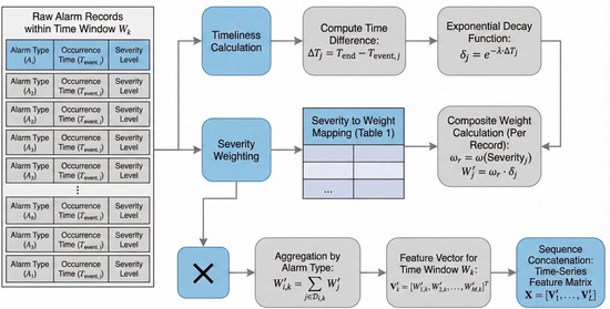
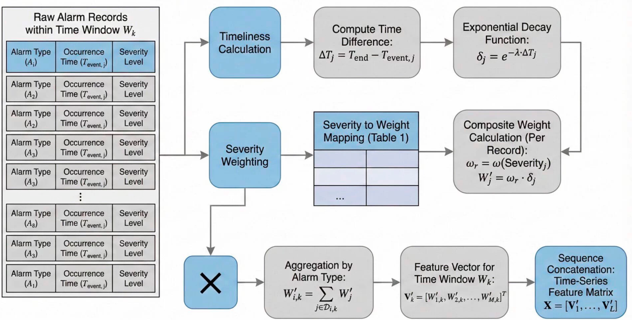
When constructing the feature vector, the traditional simple counting method (which only counts the number of alarm occurrences within the time window) ignores the significant differences in the impact of different alarms on network quality of service (QoS), and also fails to consider the different effects of the proximity of alarm occurrence time on the current fault state. To deeply embed the severity and timeliness of faults in the features, this paper proposes a composite timeliness severity weighting method. This method combines the expert domain knowledge of MCN operation and maintenance with data-driven temporal characteristics to construct a feature representation with stronger physical meaning. First, based on the MCN operation and maintenance specifications (such as the ITU-T X.733 standard [24]), alarms are classified into four severity levels ${\mathrm{S}}_{\mathrm{r}}$ (Warning, Minor, Major, Critical) according to $\mathrm{R}=4$. To reflect the importance differences numerically, the corresponding linear weights ${\mathsf{\omega }}_{\mathrm{r}}$ are assigned. Set ${\mathsf{\omega }}_{\mathrm{Critical}}$ = 4.0, ${\mathsf{\omega }}_{\mathrm{Major}}$ = 3.0, ${\mathsf{\omega }}_{\mathrm{Minor}}$ = 2.0, ${\mathsf{\omega }}_{\mathrm{Warning}}$ = 1.0. This weight allocation strategy ensures that higher-level alarms have a greater amplitude and influence in the feature space. Secondly, to reflect the timeliness of alarms, that is, the alarms that occur closer to the current time are more capable of reflecting the current state of the system, an exponential decay function is used to penalize the weights of earlier occurring alarms. Let $T_{\mathrm{e}\mathrm{n}\mathrm{d}}$ be the end time of the current time window, and $\mathsf{\Delta }{T}_j$ be the time difference between the occurrence time of a certain alarm record j and $T_{\mathrm{e}\mathrm{n}\mathrm{d}}$ Then, the time decay factor ${\delta }_j$ of this alarm is calculated as follows in Equation (11):

$${\delta }_j=e^{-\lambda \cdot \mathsf{\Delta }{T}_j},$$

(11)

Among them, λ is the attenuation rate parameter, which controls the attenuation speed of memory. Through experimental verification, in this paper, λ is set to 0.5 (with the unit being $\mathsf{\Delta }{t}^{-1}$), which means that the influence of the alarm will decay to 36.7% of the original value after approximately two time windows, thereby ensuring that the model focuses on the recent changes in network status and reducing the interference from outdated information.

Ultimately, the final composite weighted score $W_{i,k}^{\prime }$ for a specific alarm type $A_i$ within each time window $W_k$ is calculated as the sum of the severity weights of all the alarm records of this type within the window multiplied by the time decay factor, as expressed in Equation (12):

$$W_{i,k}\prime ={\sum }_{j\in {\mathcal{D}}_{i,k}}\left(\mathsf{\omega }\left({\mathrm{S}\mathrm{e}\mathrm{v}\mathrm{e}\mathrm{r}\mathrm{i}\mathrm{t}\mathrm{y}}_j\right)\cdot {\delta }_j\right),$$

(12)

Here, ${\mathcal{D}}_{i,k}$ represents the set of all alarms of type $A_i$ within the time window $W_k$. This composite score not only reflects the frequency of alarm occurrence but also integrates the severity and occurrence time of the alarms, forming the fundamental feature of high robustness, as summarized in Figure 4.

Figure 4. Timeliness structure.

5.3. Construction of the Temporal Feature Matrix X

Based on the above composite weighted and encoded form, we can construct the feature vector for each time window k as $V_k^{\prime }={\left[W_{1,k}^{\prime },W_{2,k}^{\prime },\dots ,W_{M,k}^{\prime }\right]}^T$. The final model input matrix X is composed by concatenating the feature vectors of L consecutive time windows, as shown in Equation (13):

$$X=\left[V_1\prime ,V_2\prime ,\cdots ,V_L\prime \right]\in {\mathit{R}}^{M\times L},$$

(13)

The rows M of this matrix represent different types of alarms (feature dimensions), while the columns L represent the historical time steps. This standardized temporal feature matrix X contains rich spatio-temporal semantic information, providing a solid data foundation for the subsequent model’s feature extraction and diagnosis.

6. Experiments and Analysis

6.1. Introduction to the Experimental Environment and Dataset

This experiment aims to conduct a comprehensive verification and evaluation of the performance of the TL-FDN hybrid diagnostic method. The experiment utilized the dataset from the NetAITask project, which contained 50352 alarm sequences. In terms of the distribution of alarm categories, it exhibited a natural long-tail imbalance, with the majority of state categories (such as normal state/mild fluctuation) accounting for approximately 77% of the total data, while the proportion of critical hardware failure categories was less than 2%. The data was cleaned, including removing duplicate records, handling missing values, and correcting erroneous data. The data was randomly divided into a training set, validation set, and test set, with a ratio of 7:1:2. The specific details of the hardware and software configuration for the experiment are as follows: Hardware Environment: Intel Core i9-14900HX CPU, 16 GB of RAM, and an NVIDIA GeForce RTX 5060 GPU for deep learning acceleration. Software Environment: Windows 10 operating system, Python 3.9 programming language, and PyTorch 2.8 deep learning framework. The training of all comparison models was conducted under the same hardware and software environment, data segmentation, and hyperparameter initialization conditions to ensure the fairness and effectiveness of the comparison.

6.2. Fault Diagnosis Implementation Process

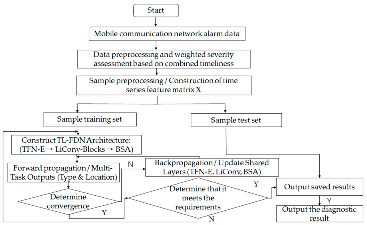
Based on the experimental environment, the fault diagnosis of the mobile communication network is completed through the process shown in Figure 5.

Figure 5. Fault Diagnosis Flowchart.

As shown in Figure 5, the main steps of mobile communication network fault diagnosis based on the improved convolutional neural network are:

• Collect mobile communication alarm data, and conduct data preprocessing and weighted severity assessment based on combined timeliness.
• Based on step 1, construct the time series feature matrix X.
• Construct the TL-FDN architecture (integrating the TFN-E module, LiConv-Blocks, and BSA mechanism) and initialize the model parameters.
• Perform forward propagation through the shared layers to extract robust features, generate the multi-task outputs (Fault Type and Fault Location), and calculate the joint loss error between the output values and the actual labels.
• Determine whether the network is convergent. If it is convergent, proceed to step 7; otherwise, move to step 6.
• The joint error value calculated in step 4 is fed back to the network, and the weights of the shared representation layers are corrected via backpropagation. Then, step 5 is entered, and the error between the network output value and the true value is calculated again. This process is repeated until the model converges.
• The network is judged based on the value of the loss function to determine whether it meets the requirements. If it does, it proceeds to step 8; otherwise, it goes to step 4 and adjusts and modifies the model parameters.
• Output of fault diagnosis results.

6.3. Selection of Experimental Setup and Evaluation Indicators

In terms of the hyperparameter settings for model training, the AdamW optimizer was adopted. This optimizer combines the adaptive learning rate of Adam and the weight decay strategy, and has better stability and convergence when dealing with the Transformer structure. The initial learning rate was set to 0.001, and the weight decay coefficient was set to 1 × 10⁻⁴. A learning rate dynamic decay strategy was employed, that is, when the loss on the validation set no longer decreases, the learning rate is halved to improve the stability of model training in the later stage and prevent model oscillation. The batch size (Batch Size) was set to 64, and the total number of iterations (Epochs) was set to 200. To prevent overfitting during training, an early stopping mechanism based on the validation set loss was adopted, with a patience value of 10. In terms of the selection of evaluation indicators, in order to comprehensively evaluate the comprehensive performance of TL-FDN, the following indicators were selected:

• Accuracy of Fault Type (${\mathrm{A}\mathrm{c}\mathrm{c}}_{\mathrm{t}\mathrm{y}\mathrm{p}\mathrm{e}}$): Measures the correctness of the model’s judgment on fault categories.
• Fault location positioning accuracy (${\mathrm{A}\mathrm{c}\mathrm{c}}_{\mathrm{l}\mathrm{o}\mathrm{c}}$): Measures the accuracy of the model in locating the area where a fault occurs.
• F1 score (F1-Score): This metric comprehensively considers the precision and recall of the model, and can better reflect the actual performance of the model in the case of class imbalance.

As shown in Table 4, to avoid subjective parameter adjustment deviations and ensure absolute fairness in benchmark comparisons, the hyperparameters in Table 3 are strictly defined based on the automated optimization mechanism. Specifically, for all deep learning models, this study constructed a unified grid search space and introduced the early stopping mechanism throughout the training process. When each model traverses the parameter boundaries, it strictly uses the highest Macro-F1 score on the independent validation set as the convergence criterion, thereby dynamically locking in their respective optimal learning rates and network capacities. At the same time, for traditional machine learning (random forest), the GridSearchCV module was called in the experiment, relying on 5-fold cross-validation of the training data to complete the parameter traversal, objectively truncating the maximum tree depth to achieve theoretical optimization of generalization ability. Moreover, for the model proposed in this paper, to align with its physical mechanism of multi-task joint optimization, the balance factor in the model objective function is directly set to 0.5. This specific configuration, from the underlying logic of gradient backpropagation, gives equal weight constraints to the “fault classification” and “fault location” dual branches.

Table 4. The configuration of all parameters of the compared algorithms.

Models	Optimizer	Learning Rate	Batch Size	Core Structural Parameters
Traditional CNN	AdamW	1 × 10−3	64	3 Conv1D layers (Channels: 64, 128, 256)
LSTM	AdamW	5 × 10−4	64	2 LSTM layers (Hidden dim: 128)
Standard Transformer	AdamW	1 × 10−3	64	4 Encoder layers; 8 Attention heads
LiConvFormer	AdamW	1 × 10−3	64	2 DSC layers; 4 Attention heads
Random Forest (RF)	-	-	-	-n_estimators:200; max_depth: 20
Rebuild the convolutional neural network	AdamW	1 × 10−3	64	1 TFN-E layer; 3 LiConv layers; 4 BSA heads; $\mathsf{\lambda }$ = 0.5

6.4. Comparative Experimental Analysis and Result Verification

In order to verify the superiority of the TL-FDN hybrid diagnostic method, four representative baseline models were selected for comparison:

• Traditional CNN: A classic network that uses stacked standard convolutional layers, representing the traditional method for extracting local features.
• LSTM: Models based on recurrent neural networks, representing the traditional methods for time series modeling.
• Standard Transformer: A model using the full attention mechanism, representing a powerful global modeling approach, but with high computational requirements.
• LiConvFormer: A current lightweight hybrid model.
• Random Forest (RF): Traditional classical machine learning algorithms

As shown in Table 5, in the fully optimized benchmark comparison, as a representative of traditional machine learning, the Random Forest (RF) algorithm is limited in its type and position accuracy performance due to its reliance on manual feature engineering and the lack of a multi-task joint learning architecture. The improved convolutional neural network proposed in this paper achieved the best performance (type accuracy rate of 98.6%, position accuracy rate of up to 98.8%). Even in the face of LiConvFormer (97.2%), which has already demonstrated excellent performance, this paper further increased the absolute accuracy rate by 1.6%. In terms of edge lightweighting, the standard Transformer performed well, but to achieve this accuracy level, its parameter quantity soared to 18.5 million, while the floating-point operation count of up to 2.24 billion made its deployment on resource-constrained edge devices extremely difficult. In contrast, the improved convolutional neural network replaced the standard attention mechanism with the broadcast self-attention mechanism (BSA), controlling the parameter quantity to 5.2 million and the floating-point operation count to only 6.8 billion. Although compared with the extremely simple traditional CNN (4.5 million), the parameter quantity increased slightly (450,000), it achieved a significant 5.4% accuracy improvement.

Table 5. Performance Comparison of Different Models in Fault Type and Location Diagnosis.

Model	Type Diagnosis Acc (%)	Type Diagnosis: Macro-F1	Position Diagnosis Acc (%)	Position Diagnosis Macro-F1	Parameter Quantity (M)	FLOPs (G)
Traditional CNN	93.2	0.921	92.1	0.910	4.5	6.5
LSTM	90.1	0.915	91.5	0.902	5.8	7.2
Standard Transformer	96.4	0.958	95.8	0.946	18.5	22.4
LiConvFormer	97.1	0.965	97.2	0.963	6.5	8.6
Random Forest (RF)	87.5	0.869	88.4	0.881	-	-
Rebuild the convolutional neural network	98.6	0.982	98.8	0.985	5.2	6.8

To verify the statistical significance of the performance improvement of the proposed model, and to eliminate the interference of accidental factors such as random initialization, this study conducted a non-parametric test. Considering that the evaluation results of multiple independent runs of deep learning usually do not follow a normal distribution, the contributions are signed-rank test that was adopted for the argumentation. In 10 independent experiments based on different random seeds, the p-values of the core indicators of the model were all strictly less than 0.05.

6.5. Feature Visualization and Qualitative Analysis

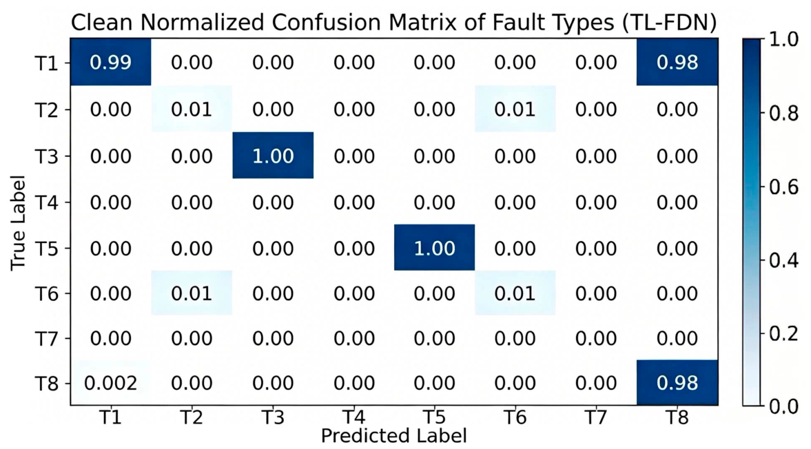
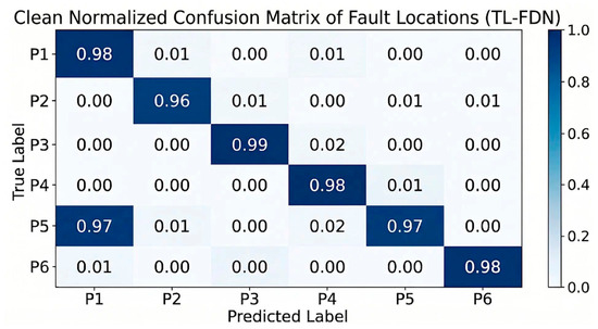
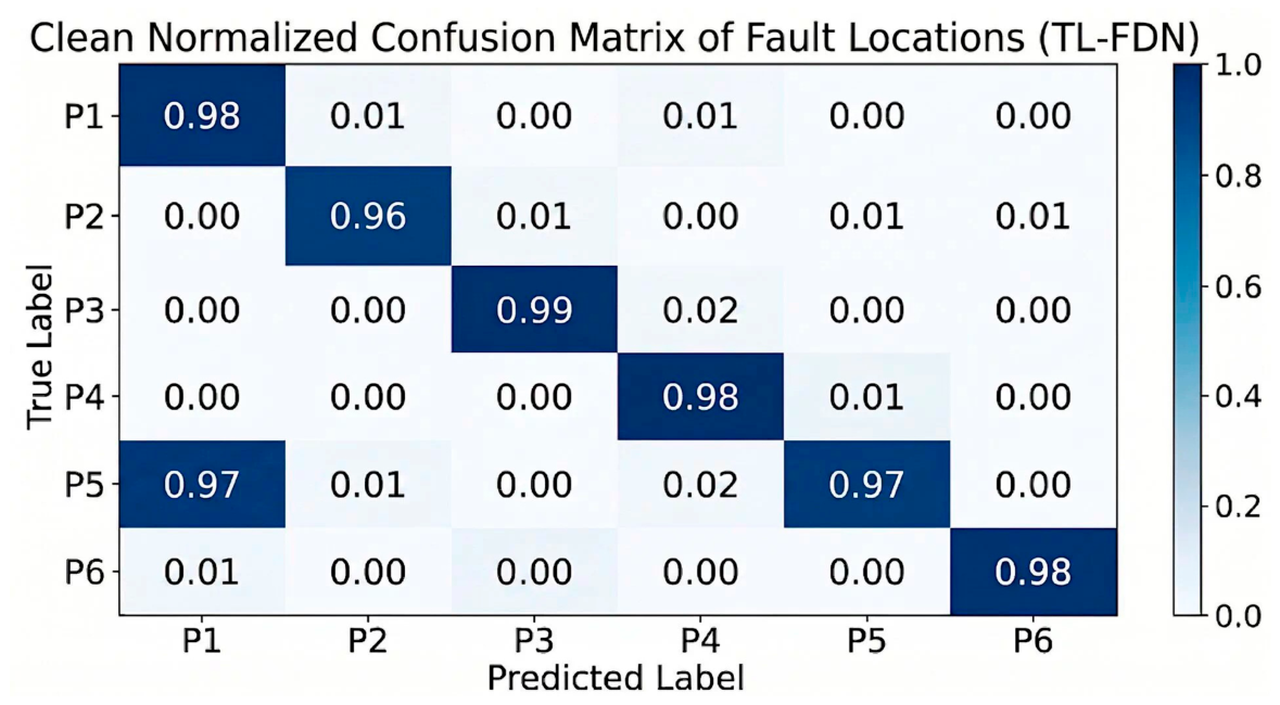
As shown in Figure 6 and Figure 7. To conduct a thorough assessment of the detailed classification performance and the robustness against data imbalance, the confusion matrices of the proposed model in the fault location and fault type tasks are presented.

Figure 6. Fault Type Normalized Confusion Matrix.

Figure 7. Fault Location Normalized Confusion Matrix.

Overall, the highly concentrated values on the main diagonal of both matrices clearly demonstrate the outstanding diagnostic accuracy of the proposed model across all independent categories. Even under severe natural long-tail imbalance conditions, the model maintains a consistently high accuracy rate in the dominant majority classes and the extreme minority classes. This proves that the model successfully overcomes the majority class bias and avoids the common defect of sacrificing the performance of minority classes for overall accuracy. These results fully validate the model’s strong generalization ability and fine-grained feature extraction capability.

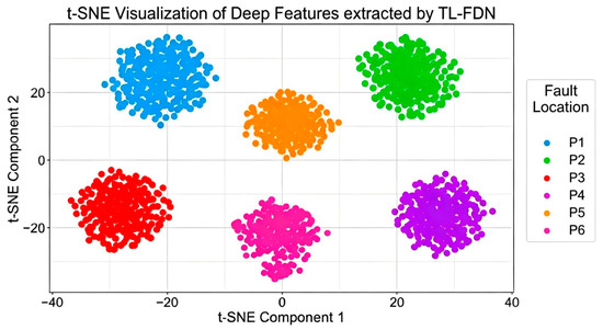
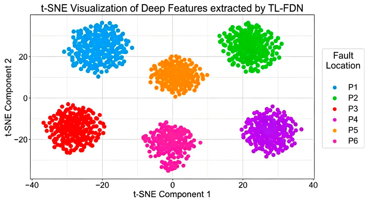
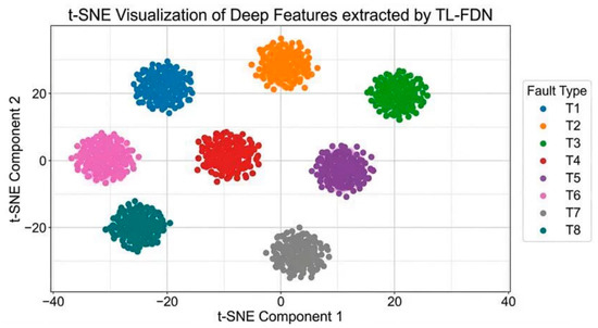
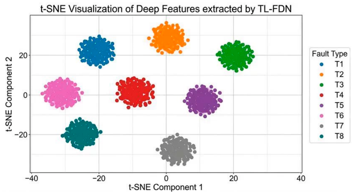
As shown in Figure 8 and Figure 9, to demonstrate the feature representation learning ability of the proposed model, t-SNE was used to project the extracted high-dimensional features into a two-dimensional visualization space. The analysis was conducted for the two tasks of fault type and fault location. The visualization results clearly showed that the feature points belonging to the same category formed highly compact clusters, while different categories were separated by clear boundaries. Despite the inherent complexity, noise, and high overlap in the original network alarm data, the model effectively decoupled these highly correlated symptom features. This effectively verified that the multi-task architecture can successfully map the complex and ambiguous input sequences to a highly discriminative feature space, thereby ensuring accurate overall diagnostic performance.

Figure 8. Fault location t-SNE feature visualization.

Figure 9. Fault type t-SNE feature visualization.

6.6. Independent Module Abolition Experiments and Analysis

In order to verify the independent performance of the core modules (TFN-E, LiConv, BSA) introduced in the improved convolutional neural network, this paper designs an ablation experiment based on the method of “gradually adding and replacing basic networks”. Here, the “basic model” refers to the network that uses standard one-dimensional convolutional layers and standard multi-head self-attention mechanisms. Taking this basic model as the benchmark, each specific innovative module is introduced or replaced, respectively, to evaluate its independent impact on diagnostic accuracy and lightweighting degree. Specifically, the defined basic model adopts the classic sequence modeling architecture, consisting of L = 6 layers of feature extraction blocks, with the hidden channel dimension of the features uniformly set to C = 128. Under this unified architecture scale, the basic model uses standard 1D convolution kernels (size K = 3) and standard global multi-head self-attention mechanisms (8 heads) as the reference anchor points for the one-by-one replacement evaluation of the modules. The quantitative results are detailed in Table 6.

Table 6. Results of the independent module ablation experiment.

Model	Structural Description	Type Diagnosis Accuracy (%)	Compared to Base Improvement	Parameter Quantity (M)	FLOPs (G)
Base (Basic Model)	Standard convolution + Standard attention	95.1	-	15.6	18.5
Base + TFN-E	Only add time-frequency feature enhancement at the front.	96.8	+1.7%	15.8	18.9
Base + LiConv	Replace only the standard convolution with the lightweight convolution	94.8	-0.3%	9.3	11.2
Base + BSA	Replace the standard attention with broadcast attention only	96.9	+1.8%	11.3	12.8
Rebuild the convolutional neural network	Integrate all three innovative modules	98.6	3.5%	5.2	6.8

Independent effect depth analysis of each module:

• The independent noise reduction gain of the TFN-E module: Compared to the base model with a higher threshold (95.1%), simply adding a learnable Gabor filter bank at the input end (Base + TFN-E) increases the type diagnosis accuracy of the model to 96.8% (+1.7%). This independently proves that, without touching the main architecture, the TFN-E module can spontaneously purify the underlying signal, filter out interference noise, and the increase in parameters (only +0.2 million) is almost negligible for the overall model capacity.
• The significant parameter compression and lightweight gain of the LiConv module: When the baseline standard convolution is replaced with the depthwise separable convolution (Base + LiConv), although there is a very slight decline in accuracy (by −0.3%) due to the decoupling of feature channels, it achieves a remarkable 40% reduction in model parameters (from 15.6 million to 9.3 million), and the computational cost (FLOPs) also drops by nearly 40% simultaneously. This set of independent test data strongly validates the core leading role of the LiConv structure in eliminating the channel redundancy of multi-dimensional temporal features and achieving engineering lightweighting.
• BSA mechanism’s independent dual-effect leap (improving accuracy and reducing consumption): By merely replacing the standard multi-head attention with the broadcast self-attention mechanism (Base + BSA), not only does the parameter quantity (reducing to 11.3 million) and FLOPs significantly decrease, but its independent introduction also leads to an impressive 1.8% increase in accuracy. This indicates that in the processing of long-sequence MCN data, BSA’s downsampling strategy is not simply sacrificing accuracy for speed, but rather forms an effective “information bottleneck”, successfully filtering out redundant local connection interference, allowing the model to focus highly on the global key dependencies.
• Model fusion synergy (TL-FDN): When these three innovative modules are seamlessly integrated into a complete architecture, the accuracy rate reaches 98.6% (a total improvement of 3.5%), while fully unlocking the potential for lightweighting, with the parameter count reduced to one-third of the baseline model (only 5.2 million). This indicates that these three modules do not operate independently but form a perfect synergy and complementarity: TFN-E provides high-quality underlying features, LiConv extracts local representations at an extremely low cost, and finally, BSA selects the global key dependencies, ultimately achieving a leapfrog improvement in both fault diagnosis accuracy and lightweighting.

6.7. Discussion

Although the comprehensive experiments have demonstrated the superiority of the proposed TL-FDN, its specific contributions and the aspects that need improvement in the future are worth in-depth exploration. (1) Identification of contributions: The fundamental contribution of TL-FDN lies in successfully balancing the trade-off between multi-task diagnostic accuracy and the deployment constraints of edge devices. The experimental ablation study shows that mapping 1D alarm signals to the 2D time-frequency domain (TFN-E) through learnable Gabor filters is the optimal strategy for dealing with non-stationary network noise. Additionally, compared with the $O\left(N^2\right)$ complexity of the standard Transformer, the proposed LiConv and BSA mechanisms effectively establish an “information bottleneck”. This enables the model to capture global fault dependencies, demonstrating its great potential in real-time MCN edge gateways. (2) Improvement space and future work: Despite these advantages, the current diagnostic framework has two main limitations, which will guide our future work. First, the multi-task loss balancing factor in this study is set as a fixed empirical value. In the highly dynamic real-world multi-device network (MCN) environment, the learning difficulty between fault type and fault location tasks may vary. Therefore, designing a dynamic adaptive weight allocation mechanism (e.g., using uncertainty-based weighting methods) is a key direction for future optimization. Second, although the model is theoretically lightweight and has been evaluated on standard computing platforms, its actual power consumption and latency on dedicated edge AI chips (such as field-programmable gate arrays or neural processing units) have not been tested. Future research will focus on hardware-aware model quantization and physical deployment tests to further verify its applicability in industry.

7. Conclusions

This research addresses the critical challenges of noise interference and computational overhead in mobile communication network (MCN) fault diagnosis. The following sections summarize the key findings, contributions, limitations and future directions of this study.

7.1. Findings and Improvements

The experimental evaluation on the NetAITask dataset provides several key findings. The proposed TL-FDN achieves a diagnostic accuracy of 98.6% for fault types and 98.8% for fault locations, representing a significant improvement (up to 5.4% accuracy gain) over traditional CNN and LSTM baselines. In terms of architectural improvements, the integration of the Gabor-based TFN-E module effectively purifies non-stationary signal noise, while the LiConv and BSA mechanisms successfully establish an “information bottleneck,” reducing the parameter count to 5.2 million—only one-third of the standard Transformer model.

7.2. Key Contributions

The primary contribution of this work is the development of a synergistic, lightweight diagnostic framework that does not rely on expert rules or physical topology. By parameterizing convolution kernels into learnable filters and optimizing global dependency modeling via broadcast self-attention, this study provides a robust solution for real-time fault diagnosis on edge gateways with limited computing resources.

7.3. Limitations

As discussed in Section 6.6, the success of TL-FDN stems from its ability to capture both localized time-frequency features and global temporal correlations. However, this study has certain limitations. The multi-task loss balancing factor $\lambda$ remains an empirical constant, and the model has yet to undergo physical stress testing on dedicated edge AI hardware (e.g., NPUs).

7.4. Future Work

Building upon these insights, future work will focus on developing an adaptive loss weighting mechanism to handle dynamic task complexities. Furthermore, we intend to implement model quantization and pruning techniques to facilitate the deployment and evaluation of TL-FDN on actual 5G/6G edge-side hardware platforms.

References

- Chen, M.; Jin, L.; Gong, X.; Man, Y. Fault Traceback Technology for Massive Network Management Data in 5G. J. Beijing Univ. Posts Telecommun. 2018, 41, 131–136. (In Chinese) [Google Scholar] [CrossRef]
- Lei, X.; Cheng, G.; Zhang, Y.; Guo, L.; Zhang, F. Alarm Information Association Analysis Based on Power Network Situation Awareness Platform. Comput. Eng. Sci. 2023, 45, 1197–1208. (In Chinese) [Google Scholar] [CrossRef]
- Ma, X.; Yang, T.; Wang, Y.; Yuan, H.; Liu, Z.; He, W. Transformer Oil Chromatography Fault Diagnosis Method Based on Lightweight Neural Network and Model Compression. Power Supply Util. 2023, 40, 84–91. (In Chinese) [Google Scholar] [CrossRef]
- Liu, Y. Research on Knowledge Graph Reasoning Decision-Making Method for Industrial Equipment Fault Diagnosis. Master’s Thesis, Nanjing University of Aeronautics and Astronautics, Nanjing, China, 2023. (In Chinese) [Google Scholar] [CrossRef]
- Li, G.; Qin, Y.; Qi, J. Fault Diagnosis of High-Speed Train Lateral Shock Absorber Based on GASF Multi-Channel Image Temporal Fusion. J. Vib. Shock. 2025, 44, 144–152. (In Chinese) [Google Scholar] [CrossRef]
- Vaswani, A.; Shazeer, N.; Parmar, N.; Uszkoreit, J.; Jones, L.; Gomez, A.N.; Kaiser, L.; Polosukhin, I. Attention is all you need. Adv. Neural Inf. Process. Syst. 2017, 30, 5998–6008. [Google Scholar] [CrossRef] [Scilit]
- Woo, G.; Liu, C.; Kumar, A.; Xiong, C.; Savarese, S.; Sahoo, D. Unified training of universal time series forecasting transformers. In Proceedings of the International Conference on Learning Representations, Vienna, Austria, 7–11 May 2024. [Google Scholar] [CrossRef] [Scilit]
- Qiang, R.; Zhao, X. A Small Sample Rolling Bearing Fault Diagnosis Method Based on Gram Angle Difference Field and Generative Adversarial Network. J. South China Univ. Technol. (Nat. Sci. Ed.) 2024, 52, 64–75. (In Chinese) [Google Scholar]
- Fang, Y.; Li, W.; Zeng, Y.; Zheng, Y.; Hu, Z.; Lu, S. Lightweight Neural Network Restoration Algorithm for Edge Deployment Scenarios. J. Comput. Sci. 2024, 47, 1383–1394. (In Chinese) [Google Scholar]
- Shan, N.; Xu, X.; Bao, X.; Ding, Q.; Liao, T. Lightweight Fault Diagnosis Method for Electromagnetic Energy Equipment Based on Edge Intelligence. Trans. China Electrotech. Soc. 2025, 40, 821–831. (In Chinese) [Google Scholar] [CrossRef]
- Wang, G.; Yang, C.; Ma, L.; Dai, W. Nonlinear Kalman Filtering Based on Gaussian-Generalized Hyperbolic Mixture Distribution. Acta Autom. Sin. 2023, 49, 448–460. (In Chinese) [Google Scholar] [CrossRef]
- Wang, J.; Zhao, X.; Zhang, C.; Wang, Y. Intelligent Edge Computing Applicable to Industrial Internet of Things Gateways. Telecommun. Technol. 2024, 64, 1653–1658. (In Chinese) [Google Scholar] [CrossRef]
- Yan, R.; Zhou, Z.; Yang, Y.; Li, Y.; Hu, C.; Tao, Z.; Zhao, Z.; Wang, S.; Chen, X. Challenges and Opportunities of Explainable Artificial Intelligence in Industrial Intelligent Diagnosis: Attribution Explanation. J. Mech. Eng. 2024, 60, 21–40. (In Chinese) [Google Scholar] [CrossRef] [Scilit]
- Qi, S. Research on RF Unit and Multi-channel Mismatch Calibration Technology Based on SDR. Master’s Thesis, University of Science and Technology of China, Hefei, China, 2024. (In Chinese) [Google Scholar] [CrossRef]
- Akter, S.; Chellappan, S.; Chakraborty, T.; Khan, T.A.; Rahman, A.; Al Islam, A.B.M.A. Man-in-the-Middle Attack on Contactless Payment over NFC Communications: Design, Implementation, Experiments and Detection. IEEE Trans. Dependable Secur. Comput. 2021, 18, 3012–3023. [Google Scholar] [CrossRef] [Scilit]
- Zhu, M.; Feng, R.; Zhang, X.; Li, P.; Su, B. High-Resolution Time-Frequency Feature Enhancement of Bowhead Whale Calls Based on Local Maximum Synchronous Extraction of Generalized S-Transforms. J. Mar. Sci. Eng. 2025, 13, 2332. [Google Scholar] [CrossRef] [Scilit]
- Chang, C.C.; Chen, W.P.; Lin, Y.W.; Lin, Y.J.; Pan, P.J. Real-Time Super Resolution Utilizing Dilation and Depthwise Separable Convolution. Eng. Proc. 2025, 92, 27. [Google Scholar] [CrossRef] [Scilit]
- Tian, R.; Li, X.; Ma, Z.; Liu, Y.; Wang, J.; Wang, C. LDformer: A parallel neural network model for long-term power forecasting. Front. Inf. Technol. Electron. Eng. 2023, 24, 1287–1301. [Google Scholar] [CrossRef] [Scilit]
- Wang, D.; Zhang, X. Dynamic Field Monitoring Based on Multitask Learning in Sensor Networks. Sensors 2019, 19, 1533. [Google Scholar] [CrossRef] [Scilit] [PubMed]
- Guo, J.; Sun, L.; Kawaguchi, T.; Hashimoto, S. Fault Diagnosis of Wire Disconnection in Heater Control System Using One-Dimensional Convolutional Neural Network. Processes 2025, 13, 402. [Google Scholar] [CrossRef] [Scilit]
- Park, C.H. MDCSformer: Multi-scale dilated contracted sub-transformer for fault diagnosis of rotating machinery. J. Comput. Des. Eng. 2026, 13, 462–485. [Google Scholar] [CrossRef] [Scilit]
- Alam, S.; Islam, R.; Fan, R.; Alam Shazid, S.; Hasan, A.S. Attention-Guided Multi-Task Learning for Fault Detection, Classification, and Localization in Power Transmission Systems. Energies 2025, 18, 6547. [Google Scholar] [CrossRef] [Scilit]
- Howard, A.G.; Zhu, M.; Chen, B.; Kalenichenko, D.; Wang, W.; Weyand, T.; Andreetto, M.; Adam, H. MobileNets: Efficient Convolutional Neural Networks for Mobile Vision Applications. arXiv 2017, arXiv:1704.04861. [Google Scholar] [CrossRef] [Scilit]
- TU-T Recommendation X.733; Information Technology—Open Systems Interconnection—Systems Management: Alarm Reporting Function; International Telecommunication Union (ITU): Geneva, Switzerland, 1992; Available online: https://www.itu.int/rec/T-REC-X.733/en (accessed on 25 March 2026).
Disclaimer/Publisher’s Note: The statements, opinions and data contained in all publications are solely those of the individual author(s) and contributor(s) and not of MDPI and/or the editor(s). MDPI and/or the editor(s) disclaim responsibility for any injury to people or property resulting from any ideas, methods, instructions or products referred to in the content. |
© 2026 by the authors. Licensee MDPI, Basel, Switzerland. This article is an open access article distributed under the terms and conditions of the Creative Commons Attribution (CC BY) license.