SSA-A-BiGCRNN: An Attention-Based Spectrum Prediction Method for Spatio-Temporal Feature Synergy

Abstract

Spectrum prediction is essential for implementing dynamic spectrum management and mitigating spectrum congestion. However, spectrum data in real electromagnetic environments exhibit high non-stationarity, multi-scale features, and complex non-Euclidean spatio-temporal coupling characteristics, which limit the prediction accuracy of existing models. To address these issues, this paper proposes an attention-based spectrum prediction method for spatio-temporal feature synergy (SSA-A-BiGCRNN). First, Singular Spectrum Analysis (SSA) is introduced to decompose and reconstruct the non-stationary spectrum signals, filtering out high-frequency burst noise and extracting core evolutionary trends. Second, a spatial topology graph among multiple frequency bands is constructed based on the Spearman rank correlation coefficient. A Bidirectional Graph Convolutional Recurrent Neural Network is then designed to simultaneously capture the spatial dependencies between frequency bands and the bidirectional evolutionary patterns in the time dimension. Finally, an attention mechanism is incorporated during the feature fusion stage to evaluate and focus on critical spatio-temporal information, further enhancing global prediction accuracy. Experimental results based on a real electromagnetic monitoring dataset demonstrate that the proposed model achieves an accuracy of 96.82%, a coefficient of determination ($R^2$) of 0.9966, a Root Mean Square Error (RMSE) of 0.5597, and a Mean Absolute Error (MAE) of 0.4031, significantly outperforming existing models.

1. Introduction

With the rapid development of 5G communication networks and Internet of Things (IoT) technologies, the massive connection of terminal devices has placed unprecedented carrying pressure on limited electromagnetic spectrum resources [1]. According to surveys by authoritative institutions such as the Federal Communications Commission (FCC), many allocated exclusive spectrum bands remain largely idle in specific times and spaces, with the average utilization rate of some bands and spectra falling below 5% [2]. To address this underutilization, Cognitive Radio (CR) was proposed [3]. Rather than relying solely on continuous, high-energy-consuming spectrum sensing, spectrum prediction technology has emerged as an active and intelligent spectrum resource management approach [4,5]. Fundamentally, the core scientific problem addressed in this study is how to accurately perform multi-step forecasting of continuous Power Spectral Density (PSD) under highly complex and non-stationary electromagnetic conditions. Unlike early studies that focused on simple binary classification (Busy/Idle) for independent channels, predicting multi-step continuous PSD requires the reconstruction of continuous signal power evolution, which is far more sensitive to real-world behaviors such as complex fading, multi-scale fluctuations, and environmental noise.

To address spectrum prediction, extensive prior works have been developed, gradually evolving from statistical models to deep learning architectures. Early spectrum prediction research primarily relied on model-driven time-series analysis methods. For example, Gorcin et al. [6] and Eltom et al. [7] utilized Autoregressive and Hidden Markov Model (HMM)-based methods. These statistical approaches rely heavily on strict data stationarity assumptions and Markovian state transitions. Consequently, the type of prediction they perform is generally limited to short-term, binary spectrum occupancy prediction (Busy/Idle). Wang et al. [8] proposed a Support Vector Machine (SVM)-based scheme, which achieved favorable performance in short-term prediction but struggled to map the highly nonlinear continuous spectrum features present in real electromagnetic environments.

To overcome the limitations of linear assumptions, data-driven deep learning methods have been widely adopted. Recurrent Neural Networks (RNNs), particularly Long Short-Term Memory (LSTM) and Gated Recurrent Unit (GRU) networks, form the foundation of temporal spectrum prediction. By utilizing gated memory mechanisms, these models effectively capture long-term temporal dependencies. These methods [9,10,11] are primarily designed to perform single-band, continuous PSD or load prediction. For instance, Soni et al. [9] and Tusha et al. [10] utilized LSTM and GRU to process real electromagnetic measurement data with lower training costs. However, real-world broadband spectrum evolution involves not only temporal dynamics but also strong spatial coupling and physical interference between frequency bands. Unidirectional temporal prediction is evidently insufficient for multi-band scenarios [12].

Consequently, recent state-of-the-art (SOTA) research has shifted toward joint spatio-temporal prediction, which serves as the primary benchmark category for validating our proposed model. Initially, researchers utilized Convolutional Neural Networks (CNNs) [13,14,15], which extract local spatial grids via convolutional kernels, enabling multi-channel joint state prediction. However, due to real-world behaviors like radio frequency (RF) device leakage and broadband modulation, inter-band correlations exhibit complex non-Euclidean topological structures that grid-based CNNs cannot perfectly align with. To address this, Graph Neural Networks (GNNs) have been introduced. Zhang et al. [16] proposed an Attention Graph Convolutional Recurrent Neural Network (A-GCRNN). It utilizes a message passing mechanism on non-Euclidean graphs, which enables the model to perform highly accurate multi-band continuous joint PSD prediction. Building upon this, Zhang et al. [17] developed SAMS-GNN to dynamically learn inter-band correlations using a multi-scale fusion strategy. Concurrently, Transformer-based architectures have emerged as powerful models due to their self-attention mechanisms capable of capturing global long-range dependencies, excelling in multi-step sequence forecasting [18]. These GNN and Transformer-based models represent the most advanced techniques in continuous spatio-temporal spectrum prediction and are therefore carefully selected as baselines in this paper.

Despite this progress, when mapping prior works to real-world behaviors, two major unresolved limitations remain in existing SOTA spatio-temporal models. Firstly, they lack sufficient robustness for long-term multi-step predictions in high-noise environments. Real-world spectral data is inherently filled with complex environmental noise. During continuous multi-step prediction, high-frequency non-stationary noise is progressively amplified layer by layer, resulting in severe error accumulation and a sharp decline in prediction accuracy [19,20,21]. Although some studies combined Singular Spectrum Analysis (SSA) with BiLSTM to mitigate noise [22], their application remains confined to 1D time-series modeling, ignoring spatial topology. Secondly, the depth of spatio-temporal synergy is limited. Most existing GCRNN models adopt a unidirectional time-flow mechanism [23,24,25], failing to simultaneously utilize the forward and backward contextual information of the global sequence. Moreover, they often lack a fine-grained dynamic weighting mechanism to focus on abrupt channel state changes.

To address high-frequency noise and insufficient spatio-temporal synergy, this paper proposes an attention-based spectrum prediction method (SSA-A-BiGCRNN). By deeply integrating data modal decomposition, bidirectional graph convolutional spatio-temporal modeling, and a dynamic attention mechanism, this paper constructs a high-precision prediction framework with strong anti-noise capabilities. Our principal conclusions demonstrate that the proposed model significantly suppresses error accumulation in long-term predictions and substantially outperforms existing mainstream models in complex channel environments. The main contributions of this paper are summarized as follows:

(1)

Introduction of SSA to construct a front-end anti-noise feature enhancement module. Instead of directly feeding raw PSD data into the spatio-temporal network, Singular Spectrum Analysis (SSA) is employed to perform multi-scale modal decomposition and energy truncation. This pre-processing effectively purifies non-stationary power fluctuations and high-frequency transient spikes, ensuring that subsequent graph networks aggregate only genuine physical correlations rather than propagating random electromagnetic interference.

(2)

Construction of BiGCRNN to achieve deep spatio-temporal synergy. A spatial topology graph is constructed using Spearman’s rank correlation to represent the non-Euclidean coupling among frequency bands. By seamlessly embedding Graph Convolutional Networks (GCN) into the Bidirectional Gated Recurrent Unit (Bi-GRU) gating mechanism, the model jointly captures cross-band interference (e.g., spectral leakage) and balances the influence between long-term fading trends and instantaneous signal bursts from a global sequence perspective.

(3)

Integration of an adaptive Attention mechanism to optimize feature aggregation. To effectively suppress feature redundancy in the bidirectional hidden states, a terminal attention mechanism is introduced. It adaptively evaluates and dynamically weights the concatenated forward and backward features, enabling the model to sharply focus on the most influential historical PSD states and critical band-to-band interactions, thereby achieving highly robust and precise spectrum forecasting in complex electromagnetic environments.

In this paper, to strictly distinguish mathematical objects, scalars are denoted by regular italic letters (e.g., $x,L,d$). Both vectors and matrices are denoted by bold letters (e.g., $\mathit{x},\mathit{X},\mathit{W}$). The domain of real numbers is represented by $\mathbb{R}$. The operator $\odot$ denotes the element-wise Hadamard product, and $\parallel$ represents the concatenation operation.

2. Materials and Methods

2.1. Overall Architecture of the Proposed Model

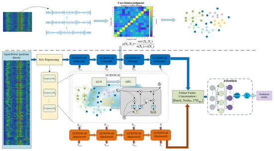
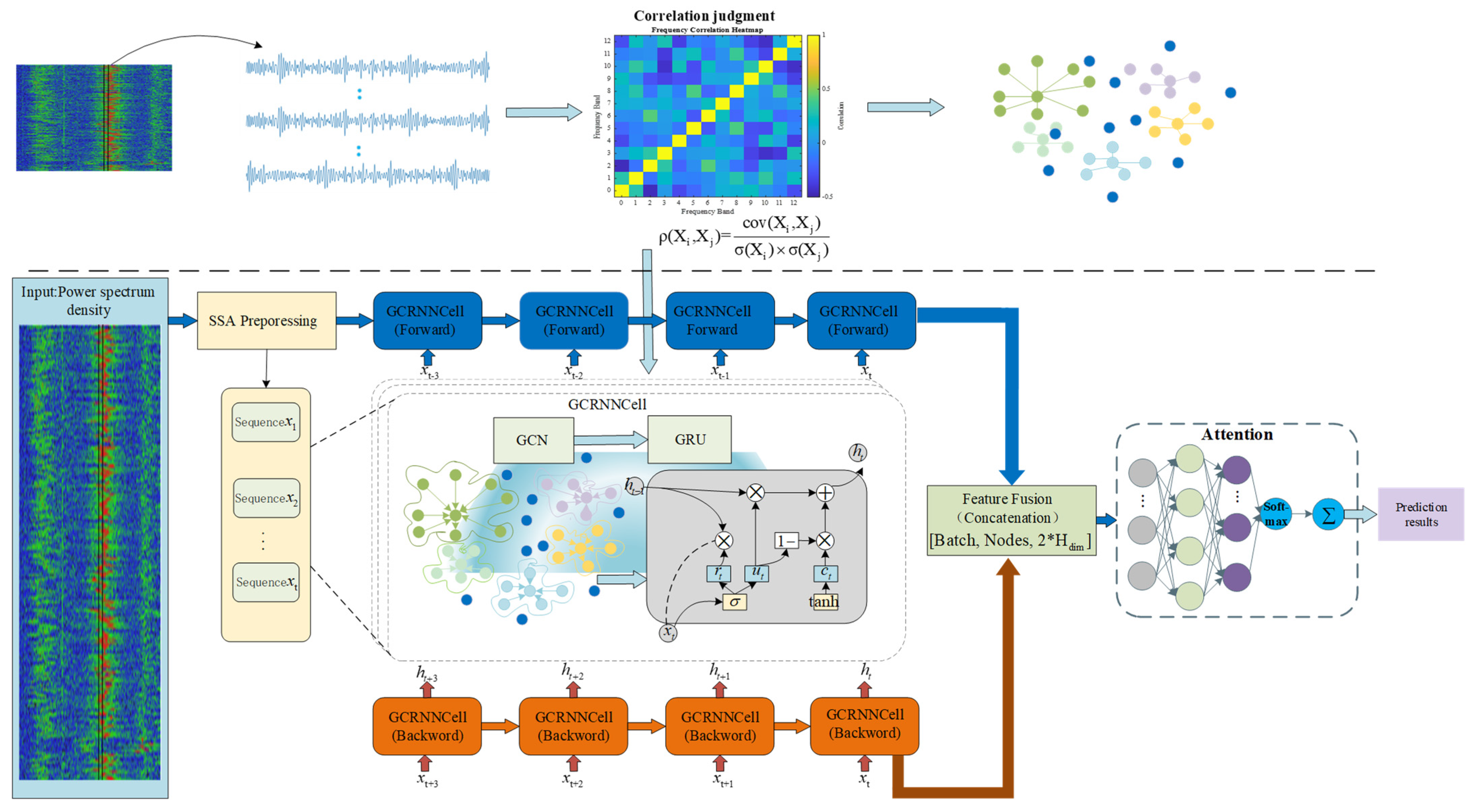
To address the complex characteristics of wireless spectrum data highlighted in the introduction—such as non-stationarity, spatial heterogeneity, and burst noise interference—traditional single prediction models often focus merely on local dimensional feature mining. These models struggle to effectively filter random environmental noise while simultaneously isolating multi-scale signal features and deeply coupling spatio-temporal bidirectional dependencies. Therefore, this paper proposes a comprehensive research framework integrating SSA preprocessing and denoising—Spatio-temporal bidirectional feature joint modeling—Attention-based adaptive weighted prediction. This framework aims to break through the prediction bottlenecks faced by existing deep learning models in complex electromagnetic environments through a multi-module synergistic mechanism. The overall architecture of the proposed model is illustrated in Figure 1, comprising four core stages:

Figure 1. Overall framework of the proposed SSA-A-BiGCRNN model.

Its core consists of the following four modules, which are closely coupled in terms of data transmission and functionality: (1) SSA denoising module: First, the raw one-dimensional spectrum observation sequences are input node by node. A trajectory matrix is constructed via a sliding local window, followed by singular value decomposition (SVD). Subsequently, based on a principal component truncation strategy, high-frequency burst noise is adaptively stripped away to accomplish smooth data reconstruction, providing high-quality stationary feature inputs for downstream networks. (2) Spatial graph structure construction module: Based on historical data sequences, the Spearman rank correlation coefficients between spectrum nodes are calculated. Through a strict threshold filtering mechanism, a binarized adjacency matrix representing strong spatial topological correlations is constructed, providing a reliable topological prior for subsequent spatial modeling. (3) Bi-GCRNN module: This module deeply integrates GCN and Gated Recurrent Units (GRU). Receiving the denoised features and spatial graph structure, it first utilizes GCN as the spatial processing unit to synchronously extract the local spatial interaction patterns of the spectrum across different monitoring nodes along the graph topology. Subsequently, the forward and backward time series are respectively passed through the GRU gating mechanism to simultaneously capture the forward historical accumulation and backward dynamic evolutionary patterns of the spectrum sequences. This ultimately realizes the deep joint modeling of bidirectional spatio-temporal features from a global perspective. (4) Attention prediction module: At the end of the network, the forward and backward hidden states at the last time step of the bidirectional network are extracted and concatenated. By introducing an Attention mechanism, the weight distribution of the multidimensional feature space is calculated. This module adaptively and dynamically focuses on key spatial nodes and deep feature channels, effectively suppressing the interference of redundant information, and finally maps and outputs high-precision spectrum prediction values.

To fully understand the proposed SSA-A-BiGCRNN, it is essential to highlight the synergistic interactions among its core modules specifically in the context of processing PSD data. First, the interaction between SSA and Bi-GCRNN prevents spatial noise broadcasting. Since real-world PSD sequences are inherently contaminated by transient power spikes and background electromagnetic noise, purifying these non-stationary power fluctuations beforehand is critical. SSA ensures that the subsequent GCN only aggregates genuine physical correlations of power distributions across frequency bands, rather than propagating random electromagnetic interference. Second, the Bi-GCRNN and Attention mechanism interact to optimize feature utilization. The bidirectional graph network extracts high-dimensional spatio-temporal dependencies from the purified PSD manifolds, while the terminal Attention adaptively screens these features to prevent information redundancy. By dynamically focusing on the most influential historical PSD states and band-to-band interactions, this cascaded interaction—PSD signal purification, graph aggregation, and dynamic weighting—forms the foundation of our robust prediction.

2.2. Singular Spectrum Analysis

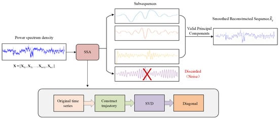
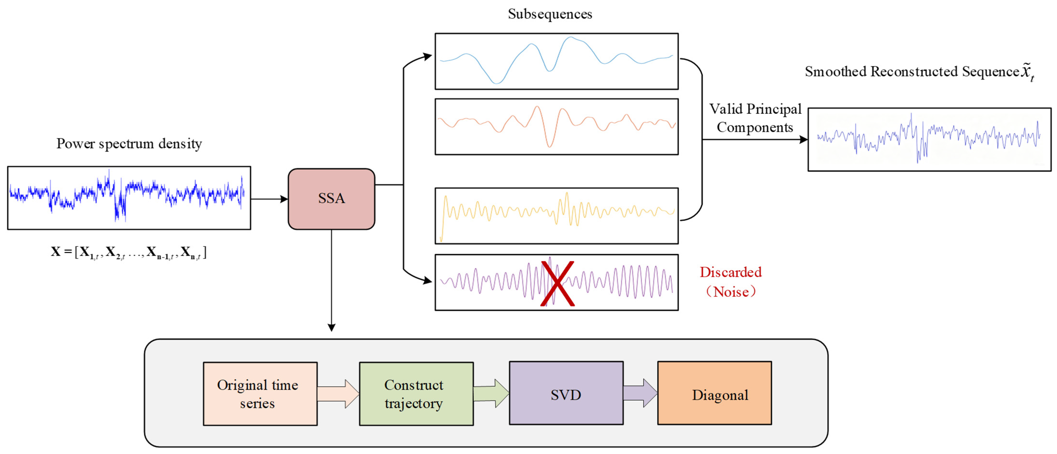
Singular Spectrum Analysis (SSA) is a nonparametric, data-driven signal processing method capable of adaptively decomposing complex, non-stationary signals into several independent feature components, such as trend, periodicity, and noise [26]. Compared with traditional linear and nonlinear filtering methods, SSA achieves adaptive signal separation in an orthogonal feature space via singular value decomposition. This effectively avoids the reliance on prior basis functions and exhibits stronger noise immunity and robustness [27]. In this paper, multi-scale decomposition and denoising using SSA are performed on the historical spectrum observation data of each frequency band. To eliminate the interference of high-frequency burst noise on prediction accuracy, this study discards noise components representing high-frequency fluctuations based on the principal component distribution characteristics of singular values. The remaining valid principal components are superimposed and reconstructed to obtain a smoothed feature sequence that retains the core evolutionary trend, serving as the input for the downstream deep prediction models. The detailed SSA processing procedure, demonstrating the decomposition, noise truncation, and final reconstruction into a single smoothed sequence, is explicitly illustrated in Figure 2. Specifically, the front-end denoising process based on SSA primarily comprises the following three core steps:

Figure 2. Procedure of the SSA.

(1)

Phase Space Embedding and Trajectory Matrix Construction

Let the original 2D PSD be denoted as $\mathit{P}\in {\mathbb{R}}^{N\times M}$, where $N$ is the total number of time steps (rows) and $M$ is the total number of frequency bands (columns). In our model, the SSA preprocessing is applied to each frequency band independently. For the $m$-th frequency band ($m\in \{1,2,\dots ,M\}$), its temporal observation sequence is extracted as a 1D real-valued column vector ${\mathit{x}}^{\left(m\right)}=[x_1^{\left(m\right)},x_2^{\left(m\right)},\dots ,x_N^{\left(m\right)}{]}^T\in {\mathbb{R}}^{N\times 1}$.

The first stage of SSA aims to map this 1D sequence into a multi-dimensional trajectory matrix through a sliding window. To simplify the notation, we drop the superscript $\left(m\right)$ and denote the sequence for any single band as $\mathit{x}=[x_1,x_2,\dots ,x_N{]}^T$. The construction process of its trajectory matrix is shown in Equation (1):

$$\mathit{X}=\left[\begin{array}{cccc}{x}_1& x_2& \dots & x_K\\ x_2& x_3& \dots & x_{K+1}\\ ⋮& ⋮& \ddots & ⋮\\ x_L& x_{L+1}& \dots & x_N\end{array}\right]\in {\mathbb{R}}^{\mathrm{L}\times \mathrm{K}}$$

(1)

where $x_t\in \mathbb{R}$ is a scalar representing the PSD observation value at time step $t$; L is the sliding window length during the embedding process; K is the number of lagged vectors, satisfying K = N − L + 1; and $\mathit{X}$ is the constructed The L × K-dimensional trajectory matrix.

(2)

Singular Value Decomposition and Energy Truncation Reconstruction

To extract the core feature components from the aforementioned trajectory matrix, Singular Value Decomposition (SVD) is introduced to project the multi-dimensional matrix into an orthogonal feature space. The components are then truncated and reconstructed based on the energy dominance ratio, as defined in Equations (2) and (3):

$${\mathit{X}}_{\mathrm{r}\mathrm{e}\mathrm{c}\mathrm{o}\mathrm{n}\mathrm{s}\mathrm{t}\mathrm{r}\mathrm{u}\mathrm{c}\mathrm{t}}={\displaystyle \sum _{i=1}^d}{\sigma }_i{\mathit{u}}_i{\mathit{v}}_i^T$$

(2)

$$d=\max (\mathrm{f}\mathrm{i}\mathrm{x}(L\times r),1)$$

(3)

where ${\sigma }_i$ is the $i$-th singular value, representing the energy proportion of the corresponding feature component; ${\mathit{u}}_i$ and ${\mathit{v}}_i$ are the corresponding column and row vectors in the left and right singular matrices, respectively; $\mathrm{f}\mathrm{i}\mathrm{x}(\cdot )$ is the round-down function; $\max (\cdot ,\cdot )$ is a function that returns the maximum of two values; $d$ is the truncation threshold, used to control the ratio of feature retention to noise filtering; and $\mathrm{r}$ is the principal component retention ratio. During this denoising and reconstruction process, the selection of the truncation threshold is crucial to the final reconstruction effect. To enhance the adaptability of parameter setting and simplify the hyperparameter optimization process, this paper formulates the calculation of the truncation threshold $\mathrm{d}$ as a function of the window length $L$ and the retention ratio $r$.

(3)

Diagonal Averaging and Time-Series Restoration

The feature representation after truncation and reconstruction remains a two-dimensional matrix, which needs to be mapped and restored to a one-dimensional sequence in the time domain using the diagonal averaging operation. This operation calculates the reconstructed smoothed sequence ${\tilde{x}}_{\mathrm{t}}$ at the $\mathrm{t}$-th time step by finding the mean of the elements on each anti-diagonal. Its iterative calculation formula is shown in Equation (4):

$${\tilde{x}}_t={\displaystyle \frac{1}{w_{\mathrm{t}}}}\sum _{(i,j)\in S_t}{x}_{i,j}^{*}$$

(4)

where $x_{i,j}^{*}$ is the corresponding element in the denoised reconstruction matrix ${\mathit{X}}_{\mathrm{r}\mathrm{e}\mathrm{c}\mathrm{o}\mathrm{n}\mathrm{s}\mathrm{t}\mathrm{r}\mathrm{u}\mathrm{c}\mathrm{t}}$; $S_t=\left\{\right(i,j)\mid i+j-1=t\}$ represents the set of elements in the matrix whose sum of subscripts corresponds to time $\mathrm{t}$; and ${\mathrm{w}}_{\mathrm{t}}$ is the total number of elements contained in this set.

This diagonal averaging mapping process is performed step by step over time until the entire sequence length is traversed. Ultimately, the raw spectrum signal containing high-frequency jitter is successfully reconstructed into a smooth time-series evolutionary sequence with true physical significance, which is directly fed into the back-end deep learning network.

2.3. Construction of Frequency Band Correlation Graph Structure

Spectrum data exhibits not only dynamic variability in the temporal dimension but also significant topological dependencies in the frequency dimension. Driven by similar radio propagation environments or user behavior patterns, different sub-bands often demonstrate highly coordinated spatio-temporal fluctuation characteristics. To deeply mine these potential spatial coupling relationships, this paper uniformly models the multi-band spectrum prediction task as a graph structure learning problem in a non-Euclidean space. The spectrum graph structure is defined as $G=(V,E)$, where $V$ represents the set of $N$ sub-band monitoring nodes, and $E$ represents the set of edges indicating the connection relationships between nodes. Considering the nonlinear distribution characteristics of spectrum data, this paper selects the Spearman rank correlation coefficient as the metric for monotonic correlation between nodes [28]. In the specific calculation, the algorithm first maps the raw data into ranks, and then calculates the correlation between the rank sequences. For any two frequency band nodes $i$ and $j$, with corresponding historical observation sequences ${\mathit{X}}_i$ and ${\mathit{X}}_j$, they are transformed into rank sequences $R\left({\mathit{X}}_i\right)$ and $R\left({\mathit{X}}_j\right)$. The Spearman rank correlation coefficient between them is defined as shown in Equation (5):

$${\rho }_{spearman}(i,j)={\displaystyle \frac{cov\left(R\right({\mathit{X}}_i),R({\mathit{X}}_j\left)\right)}{\sigma \left(R\right({\mathit{X}}_i\left)\right)\times \sigma \left(R\right({\mathit{X}}_j\left)\right)}}$$

(5)

where $cov\left(R\right({\mathit{X}}_i), R({\mathit{X}}_j\left)\right)$ is the covariance between the rank sequences $R\left({\mathit{X}}_i\right)$ and $R\left({\mathit{X}}_j\right)$, and $\sigma \left(R\right({\mathit{X}}_i\left)\right)$ and $\sigma \left(R\right({\mathit{X}}_j\left)\right)$ are the standard deviations of their respective rank sequences.

Based on the calculated correlation coefficient matrix, a binarized adjacency matrix is constructed by setting a strict threshold $\tau$ to filter out noise interference and retain strong correlation connections. When the correlation coefficient is greater than the threshold $\tau$, it is considered that a significant monotonic dependence exists between the frequency bands; otherwise, they are regarded as uncorrelated. The construction rule for the adjacency matrix $A$ is shown in Equation (6):

$${\mathit{A}}_{ij}=\{\begin{array}{ll}1,& if {\rho }_{spearman}(i,j)>\tau \\ 0,& otherwise\end{array}$$

(6)

To preserve the nodes’ own feature states in the subsequent graph convolution operations, this paper further introduces self-loops to the adjacency matrix, i.e., constructing $\tilde{\mathit{A}}=\mathit{A}+\mathit{I}$. Subsequently, based on the adjacency matrix with self-loops, the normalized Laplacian matrix $\widehat{L}$ is calculated and serves as the final mathematical representation of the spatial graph topology. The definition of the Laplacian matrix is shown in Equation (7):

$$\widehat{\mathit{L}}={\tilde{\mathit{D}}}^{-{\displaystyle \frac{1}{2}}}\tilde{\mathit{A}}{\tilde{\mathit{D}}}^{-{\displaystyle \frac{1}{2}}}$$

(7)

where $\tilde{\mathit{D}}$ is the degree matrix containing self-loops, and its diagonal elements satisfy ${\tilde{\mathit{D}}}_{ii}=\sum _j{\tilde{\mathit{A}}}_{ij}$; $\mathit{I}$ is the identity matrix.

Through the above process, the model successfully constructs a graph structure representation that characterizes the topological relationships and spatial feature attributes between frequency bands, laying a solid mathematical foundation for spatial feature extraction in the subsequent Bi-GCRNN.

2.4. Bidirectional Graph Convolutional Recurrent Neural Network (BiGCRNN) Model

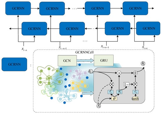
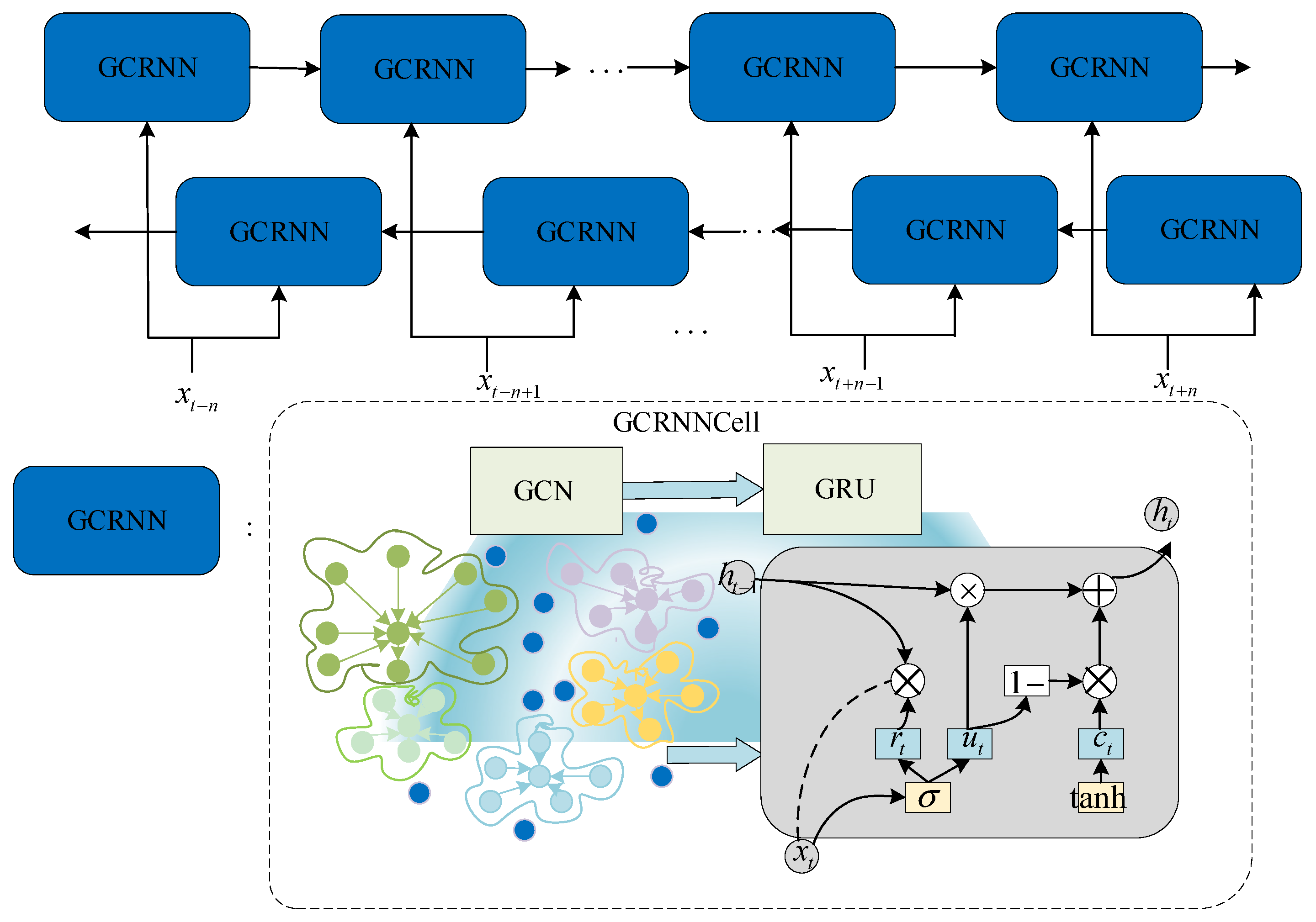
Bi-GCRNN is a neural network architecture that deeply fuses graph topological spatial features with sequential temporal dynamic evolutionary patterns. Compared to LSTM, GRU has advantages such as fewer parameters in time-series processing. However, time-series prediction models like GRU can only independently capture the temporal dependencies of a single node, making it difficult to handle the complex non-Euclidean spatial topological correlations among multiple frequency bands [29]. Therefore, this paper takes the extracted frequency band spatial graph structure and the denoised spectrum time-series features as inputs, utilizing the Bi-GCRNN module for joint spatio-temporal modeling. To simultaneously aggregate spatial interaction information and temporal evolutionary features, this module seamlessly embeds GCN operations into the gating calculation mechanism of a standard GRU. Specifically, to clarify its internal hierarchical structure, the processing flow consists of two highly integrated sub-components: first, the GCN acts as the spatial feature extractor, utilizing the pre-constructed Spearman adjacency matrix to aggregate cross-band topological correlations; subsequently, these spatially enhanced node representations are channeled directly into the GRU’s update and reset gates to model long-range temporal dependencies. This organically combines the aggregation of local spatial topological features with the update of global temporal states. Its internal hidden layer structure is illustrated in Figure 3.

Figure 3. Hidden layer structure of BiGCRNN.

The gating mechanism and graph convolutional feature aggregation process within the GCRNN unit are shown in Equations (8)–(10b):

$${\mathbf{r}}_{\mathrm{t}}=\mathsf{\sigma }\left({\mathit{W}}_{\mathrm{r}}{\ast }_{\mathcal{G}}\right[{\mathit{X}}_{\mathrm{t}},{\mathit{h}}_{\mathrm{t}-1}]+{\mathit{b}}_r)$$

(8)

$${\mathit{u}}_{\mathrm{t}}=\mathsf{\sigma }\left({\mathit{W}}_u{\ast }_{\mathcal{G}}\right[{\mathit{X}}_t,{\mathit{h}}_{t-1}]+{\mathit{b}}_u)$$

(9)

$${\mathit{c}}_{\mathrm{t}}=\tanh ({\mathit{W}}_{\mathrm{c}}{\ast }_{\mathcal{G}}[{\mathit{X}}_t,({\mathit{r}}_t\odot {\mathit{h}}_{t-1}\left)\right]+{\mathit{b}}_c)$$

(10a)

$${\mathit{h}}_t={\mathit{u}}_{\mathit{t}}\odot {\mathit{h}}_{t-1}+(1-{\mathit{u}}_t)\odot {\mathit{c}}_t$$

(10b)

where ${\mathit{X}}_t$ is the denoised spectrum feature input at time $t$; ${\mathit{h}}_{t-1}$ and ${\mathit{h}}_{\mathit{t}}$ are the hidden states at the previous and current time steps, respectively; ${\mathit{r}}_{\mathit{t}}$ and ${\mathit{u}}_t$ are the reset gate and update gate, respectively; ${\mathit{c}}_t$ is the candidate hidden state; $\mathsf{\sigma }$ and $\mathrm{t}\mathrm{a}\mathrm{n}\mathrm{h}$ represent the Sigmoid and hyperbolic tangent activation functions, respectively; $\odot$ denotes the Hadamard product of matrix elements; ${\ast }_{\mathcal{G}}$ represents the graph convolution aggregation operation executed based on the normalized Laplacian matrix $\widehat{\mathit{L}}$; and $\mathit{W}$ and $b$ are the learnable weight matrices and bias parameters in the network.

To align the generic neural network operations with the physical characteristics of spectrum dynamics, the components in Equations (8)–(10b) are interpreted within the context of CR systems:

Spatial Coupling Representation: The graph convolution operation ${\ast }_{\mathcal{G}}$ utilizes the normalized Laplacian matrix $\widehat{\mathit{L}}$, which is constructed from the spectral correlation coefficients between frequency bands. Unlike standard GRU, this operation enables the unit to capture inter-band interference and spectral leakage—physical phenomena where the power distribution of one band is topologically coupled with its neighbors.

Gating Mechanism for Non-stationary Fading: The reset gate ${\mathit{r}}_t$ and update gate ${\mathit{u}}_t$ serve as adaptive filters. In a high-noise electromagnetic environment, ${\mathit{r}}_t$ dynamically determines how much “historical interference” from ${\mathit{h}}_{t-1}$ should be discarded, while $u_t$ balances the influence between long-term fading trends and instantaneous signal bursts in the current PSD input ${\mathit{X}}_t$.

Spatiotemporal State Evolution: The hidden state ${\mathit{h}}_t$ is not merely a numerical vector but represents the latent spectral state. By embedding GCN into the GRU cell, the model achieves a recursive update of the global electromagnetic environment, allowing the prediction to be informed by both the temporal evolution of signal power and the spatial topology of the spectrum.

Furthermore, a single forward sequence evolution often ignores the feedback constraints of future states on the current evolutionary trend. To comprehensively capture the bidirectional dependency patterns of spectrum states in the temporal dimension, this paper introduces a bidirectional architecture, utilizing two independent GCRNN units to perform iterative calculations along the forward and backward directions of the time series, respectively. The forward network accumulates evolutionary features in chronological order from history to future, while the backward network extracts feedback features in reverse chronological order from future to history. The iterative updates of the forward and backward hidden layer states are shown in Equations (11) and (12):

$${\overrightarrow{\mathit{h}}}_t={GCRNN}_{forward}({\mathit{X}}_t,{\overrightarrow{\mathit{h}}}_{t-1})$$

(11)

$${\overleftarrow{\mathit{h}}}_t={GCRNN}_{backward}({\mathit{X}}_t,{\overleftarrow{\mathit{h}}}_{t+1})$$

(12)

where ${GCRNN}_{forward}$ and ${GCRNN}_{backward}$ represent the forward and backward graph convolutional recurrent processing units, respectively; ${\overrightarrow{\mathit{h}}}_t$ is the historically accumulated hidden state extracted by the forward network at time $t$; and ${\overleftarrow{\mathit{h}}}_t$ is the future feedback hidden state extracted by the backward network at time $t$.

This bidirectional iterative process continues until all time steps of the input sequence are traversed. Through the above mechanism, the model successfully deep-couples the complex spatial interaction patterns among frequency bands with the bidirectional dependencies of long- and short-term time series. At the end of the network, the model extracts and concatenates the final forward and backward hidden states at the last time step of the bidirectional network. This operation not only effectively condenses the spatio-temporal evolutionary information of the global sequence but also provides a multi-dimensional deep spatio-temporal fused feature representation for subsequent attention feature weighting and accurate prediction.

2.5. Attention Mechanism and Prediction Output

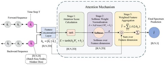
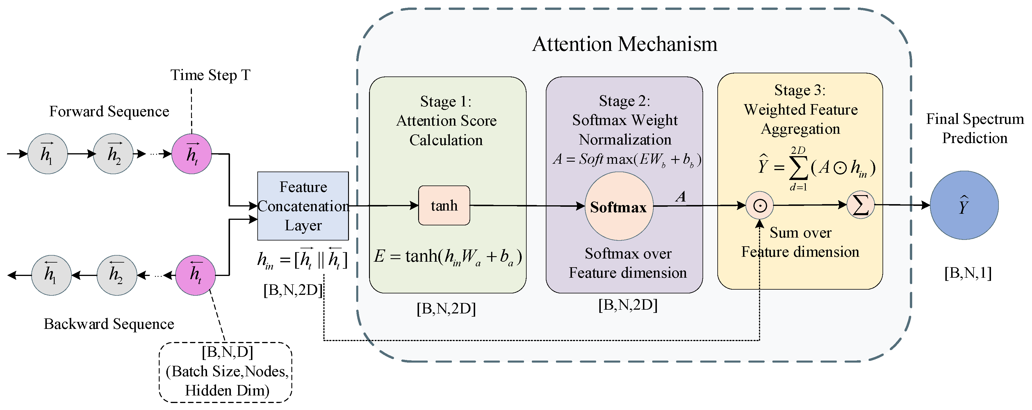
Through the joint spatio-temporal modeling of Bi-GCRNN, the model has successfully extracted high-dimensional hidden layer features containing spatial topological interactions and global temporal evolutionary patterns. However, in the deep feature space output by the bidirectional network, the contribution degrees of different feature dimensions to the final spectrum prediction results vary significantly. To effectively suppress feature redundancy and adaptively focus on the core representations, this paper introduces an Attention Mechanism at the end of the network to dynamically weight and aggregate-map the bidirectional fused features. The internal architecture of the attention mechanism and the prediction output process are illustrated in Figure 4.

Figure 4. Detailed architecture of the attention mechanism for bidirectional spatio-temporal feature aggregation.

Specifically, the execution of this mechanism can be divided into three core stages.

First, based on the iterative process of the bidirectional network, the model extracts the historically accumulated hidden state ${\overrightarrow{\mathit{h}}}_t$ of the forward network at the last time step $t$ and the future feedback hidden state ${\overleftarrow{\mathit{h}}}_t$ of the backward network at the corresponding time step, and concatenates them along the feature dimension to construct a joint spatio-temporal feature representation ${\mathit{h}}_{in}$ containing complete global context information. This feature concatenation process is shown in Equation (13):

$${\mathit{h}}_{in}=[{\overrightarrow{\mathit{h}}}_t||{\overleftarrow{\mathit{h}}}_t]$$

(13)

where $\left|\right|$ denotes the concatenation operation along the feature dimension; the dimension of the concatenated joint feature ${\mathit{h}}_{in}$ is expanded to twice the dimension of the unidirectional hidden layer, comprehensively representing the spatio-temporal state of the current frequency band node under a global perspective. The joint feature ${\mathit{h}}_{in}$ is then fed into the attention layer.

Second, to quantify the importance of different feature dimensions, the model introduces learnable parameter matrices ${\mathit{W}}_a$ and ${\mathit{b}}_a$. The joint feature sequence is first mapped to a preliminary attention score $\mathit{E}$ via linear transformation and matrix multiplication, and then normalized using the softmax function to generate an adaptive attention weight distribution matrix $\mathit{A}$. The calculation of this process is shown in Equations (14) and (15):

$$\mathit{E}=\tanh ({\mathit{h}}_{in}{\mathit{W}}_a+{\mathit{b}}_a)$$

(14)

$$\mathit{A}=Softmax(\mathit{E}{\mathit{W}}_b+{\mathit{b}}_b)$$

(15)

where $W_a$, $W_b$, and the bias terms $b_a$, $b_b$ are the learnable network parameters within the attention mechanism; $E$ is the preliminary attention score after non-linear activation; and $\mathit{A}$ is the generated attention weight after normalization.

Finally, the calculated attention weight matrix $\mathit{A}$ is used to adaptively weight the original joint feature ${\mathit{h}}_{in}$, and an aggregation summation operation is performed along the feature dimension, thereby smoothly mapping the high-dimensional spatio-temporal hidden state into a single-dimensional predicted value. The final spectrum prediction output $\widehat{\mathit{Y}}$ is calculated as shown in Equation (16):

$$\widehat{\mathit{Y}}=\sum (\mathit{A}\odot {\mathit{h}}_{in})$$

(16)

where $\odot$ denotes the element-wise multiplication of matrices; $\sum$ represents the summation operation along the feature dimension; and $\widehat{\mathit{Y}}$ is the final spectrum prediction result output by the model for each monitoring node.

Through the concatenation and attention weighting processes, the model not only achieves the deep fusion of forward historical accumulation and backward future feedback, but also extracts the core feature components that are most valuable for prediction in a data-driven manner, thereby significantly improving the accuracy and robustness of spectrum state prediction in complex electromagnetic environments. Based on the detailed description of the key components above, this paper outlines the overall training and prediction procedure of the proposed framework, as detailed in Algorithm 1.

Algorithm 1: Training and Prediction Procedure of the SSA-A-BiGCRNN

Input: Raw non-stationary spectrum sequence $\mathit{X}$, SSA window length $L$, principal component ratio $r$, Spearman correlation threshold $\tau$, model hyperparameters $\mathsf{\Theta }$ Output: Predicted spectrum values $\widehat{\mathit{Y}}$ 1: Stage 1: SSA-based Signal Decomposition and Denoising 2: for each spectrum sequence $x$ in X do 3:   Map the 1D sequence into a multi-dimensional trajectory matrix via phase space embedding with window $L$. 4:   Perform Singular Value Decomposition (SVD) on the covariance matrix to obtain singular values and orthogonal eigenvectors. 5:   Compute the truncation threshold $d = \max (\mathit{fix}(L \times r),1)$. 6:   Select the top $d$ principal components to reconstruct the denoised matrix ${\mathit{X}}_{\mathit{reconstruct}}$. 7:   Apply diagonal averaging to map ${\mathit{X}}_{\mathit{reconstruct}}$ back to a smoothed 1D sequence ${\tilde{x}}_t$. 8: end for 9: Generate the refined feature matrix ${\tilde{\mathrm{x}}}_{\mathrm{t}}$ containing all denoised sequences. 10: Stage 2: Adaptive Graph Topology Learning 11: Calculate the pairwise Spearman rank correlation matrix ${\rho }_{\mathit{spearman}}$ among different frequency band nodes. 12: Construct the adjacency matrix $\mathit{A}$ by applying threshold $\tau :{\mathit{A}}_{\mathit{ij}} = 1$ if ${\rho }_{\mathit{spearman}}(i,j) > \tau$, else $0$. 13: Add self-loops to the adjacency matrix: $\tilde{\mathit{A}} = \mathit{A} + I$. 14: Compute the degree matrix $\tilde{\mathit{D}}$ and the normalized Laplacian matrix $\widehat{L} = {\tilde{\mathit{D}}}^{-{\displaystyle \frac{1}{2}}}\tilde{\mathit{A}}{\tilde{\mathit{D}}}^{-{\displaystyle \frac{1}{2}}}$ for graph convolution. 15: Stage 3: Spatiotemporal Representation and Attention Fusion 16: Initialize the parameters of Bi-GCRNN and the Attention layer. 17: while training stopping criteria (e.g., max epochs or early stopping) are not met do 18:   // Forward Propagation Phase 19:   Bidirectional Spatiotemporal Modeling: 20:   for each time step $t$ do 21:     Forward Pass: Capture temporal evolution and spatial dependencies via ${\overrightarrow{\mathit{h}}}_t = {\mathit{GCRNN}}_{\mathit{forward}}({\tilde{\mathit{X}}}_t,{\overrightarrow{\mathit{h}}}_{t-1})$. 22:     Backward Pass: Capture reverse-time dependencies via ${\overleftarrow{\mathit{h}}}_t={\mathit{GCRNN}}_{\mathit{backward}}({\tilde{\mathit{X}}}_t,{\overleftarrow{\mathit{h}}}_{t+1})$. 23:   end for 24:   Feature Concatenation: Merge the final bidirectional hidden states ${\mathit{h}}_{\mathit{in}} = [{\overrightarrow{\mathit{h}}}_t\left|\right|{\overleftarrow{\mathit{h}}}_t]$. 25:   Attention-based Refinement: 26:   Compute attention score and weight distribution matrix $A=\mathit{Softmax}\left(\tanh ({\mathit{h}}_{\mathit{in}}{\mathit{W}}_a + {\mathit{b}}_a\right){\mathit{W}}_b +{ \mathit{b}}_b)$. 27:   Prediction Output: Generate the estimated values $\widehat{\mathit{Y}} = \sum (\mathit{A}\odot {\mathbf{h}}_{\mathit{in}})$ through the output layer. 28:   // Backward Propagation Phase 29:   Compute the Mean Squared Error (MSE) loss function between predicted $\widehat{\mathit{Y}}$ and ground truth $\mathit{Y}$. 30:   Update model parameters $\mathsf{\Theta }$ using the Adam optimizer via back propagation. 31: end while 32: return The well-trained model and final predicted spectrum values $\widehat{\mathit{Y}}$.

3. Experimental Results and Analysis

3.1. Dataset and Experimental Settings

To ensure the reproducibility of our results, all experiments and inference benchmarks were conducted on a high-performance workstation equipped with an NVIDIA RTX 5000 GPU. The software stack was built on Python 3.9.25 and PyTorch 2.5.0, leveraging CUDA 12.1 and cuDNN 90100 for high-efficiency hardware acceleration. Data preprocessing and statistical analysis were implemented using NumPy 2.0.1, Pandas 2.3.3, and SciPy 1.13.1. Specifically, the average training time for the proposed SSA-A-BiGCRNN was approximately 384 s per run. To ensure statistical reliability, all experiments were repeated three times using different random seeds, and the average results are reported. Under this configuration, the model demonstrated robust numerical stability and met the real-time requirements for spectrum forecasting.

To comprehensively evaluate the effectiveness of the proposed model and verify its generalization capability across different electromagnetic environments, we conduct experiments on two real-world PSD monitoring datasets.

Dataset 1 is sourced from a sensor deployed in Madrid, Spain, provided by the cloud-based open-source platform Electrosense [30]. The selected frequency band ranges from 500 MHz to 800 MHz with a frequency resolution of 2 MHz, resulting in 151 distinct frequency sub-bands. According to the European Frequency Allocation Table, this sub-GHz spectrum exhibits rich radio activities, including broadcasting, television, and mobile communication services. The temporal resolution is 15 min, capturing macroscopic spectrum usage trends over one month.

To avoid overfitting to a single scenario, we introduce Dataset 2. This dataset consists of measurements collected in a residential district in Aachen, Germany, provided by RWTH Aachen University [31]. In contrast to Dataset 1, we specifically isolated a highly dynamic 60 MHz segment in the C-band, ranging from 3750 MHz to 3810 MHz. This frequency range is heavily used by modern 5G New Radio (NR) networks, showing completely different channel occupancy behaviors and non-stationary volatility compared to the sub-GHz band. Dataset 2 is divided into 300 spatial nodes (sub-bands) with a fine frequency resolution of 0.2 MHz. Moreover, it has a very high temporal sampling rate of 1.8 s, recording 6000 consecutive time steps within a 3 h window. Both datasets are split 8:2 into training and testing sets. To show generalizability, all key hyperparameters (sliding window size L = 8, retention ratio r = 0.3, and Spearman correlation threshold τ = 0.94) are kept identical. The model’s success under this unified threshold confirms that the threshold effectively extracts topological correlations regardless of frequency or sampling rate. Table 1 summarizes dataset details and hyperparameters.

Table 1. Main parameters of dataset and experiment.

Object	Parameters	Dataset1	Dataset2
Dataset	Frequency band	500–800 MHz	3750 MHz–3810 MHz
	Monitoring time	28 May 2021–28 June 2021	3 h (started 3 July 2007)
	Frequency resolution	2 MHz	0.2 MHz
	Time resolution	15 min	1.8 s
	The dimensionality of samples	151 × 2880	300 × 6000
Experiment	Dataset split ratio	8:2	8:2
	Time step	16	16
	Batch size	64	64
	Maximum epochs	300	300
	Learning rate	0.0005	0.0005
	Hidden dimension	100	100
	Correlation threshold	0.94	0.94
	Window size	8	8
	Ratio	0.3	0.3

3.2. Evaluation Metrics

We evaluate the proposed model using four evaluation criteria [5] defined in Equations (17)–(20): Accuracy, MAE, RMSE, and $R^2$.

$$Accuracy=1-{\displaystyle \frac{\Vert Y-\widehat{Y}{\Vert }_F}{\Vert Y{\Vert }_F}}$$

(17)

$$MAE={\displaystyle \frac{1}{N}}{\displaystyle \sum _{k=1}^N}|y_k-{\widehat{y}}_k|$$

(18)

$$RMSE=\sqrt{{\displaystyle \frac{1}{N}}{\displaystyle \sum _{k=1}^N}(y_k-{\widehat{y}}_k{)}^2}$$

(19)

$$R^2=1-{\displaystyle \frac{{\displaystyle {\sum }_{k=1}^N}(y_k-{\widehat{y}}_k{)}^2}{{\displaystyle {\sum }_{k=1}^N}(y_k-\overline{y}{)}^2}}$$

(20)

where ${\mathrm{y}}_k$ is the ground truth value at the $\mathrm{k}$-th time step, ${\widehat{\mathrm{y}}}_k$ is the predicted value at the $\mathrm{k}$-th time step, and $\overline{\mathrm{y}}$ is the mean of the ground truth values. These variables hold the same meaning across all four formulas above. $\mathrm{N}$ represents the total number of predicted samples, and $\Vert \cdot {\Vert }_{\mathrm{F}}$ denotes the Frobenius norm.

3.3. Comparative Experiments and Results Analysis

Among the above evaluation metrics, Accuracy measures the overall similarity between the predicted and ground truth values; a value closer to 1 indicates a more precise prediction effect. MAE measures the average of the prediction deviations; a smaller value indicates stronger model robustness. RMSE is more sensitive to larger errors and reflects the average deviation between predicted and ground truth values. $R^2$ measures the degree to which the model fits the variance of the ground truth values; a value closer to 1 represents a better fitting effect.

To evaluate the proposed SSA-A-BiGCRNN framework, we compared it against several mainstream baseline models, categorized into three structural groups:

(1)

Level 1: Classical Spatio-Temporal Hybrid Models. This category includes foundational architectures such as CNN + LSTM [13], which utilize convolutional kernels to extract local spatial features and LSTM to capture temporal dependencies.

(2)

Level 2: Global Sequence and Attention-based Architectures. To evaluate the impact of long-range dependency modeling, we included the Transformer [18], which relies on self-attention for global context perception, and Seq2seq-Bi-ConvLSTM-attention [32], which integrates bidirectional perception with attention mechanisms. Additionally, SSA-A-BiLSTM [22] is compared to assess the performance of denoising-enhanced temporal networks.

(3)

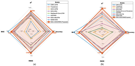
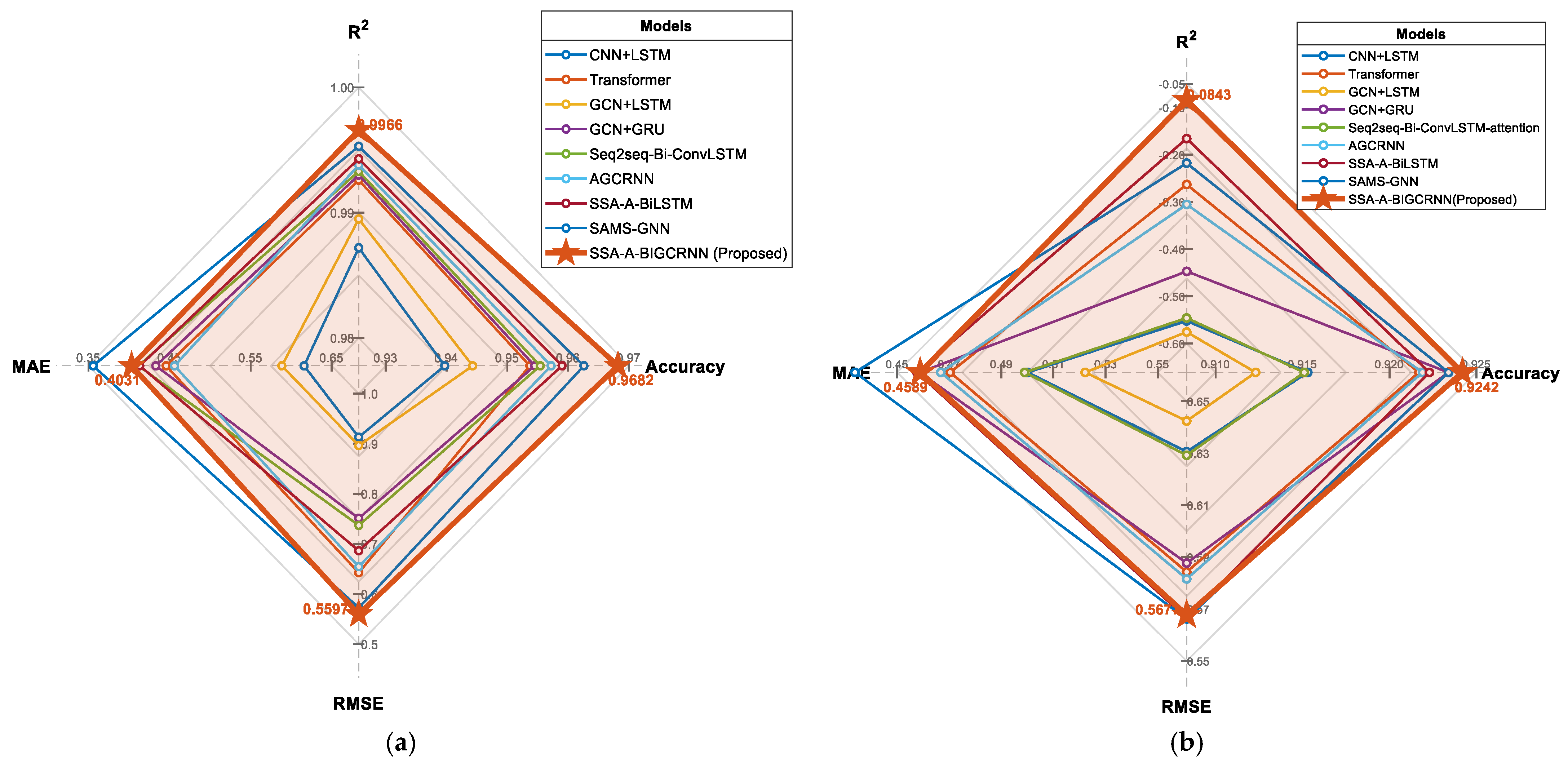
Level 3: Graph-centric and Adaptive Modeling. Focusing on the non-Euclidean topological correlations of frequency bands, this group includes GCN + LSTM [33], GCN + GRU [34], and AGCRNN [16]. This level also incorporates SAMS-GNN [17], which employs a self-adaptive graph structure and multi-scale learning to capture dynamic inter-band dependencies. The comparison results are shown in Table 2 and Figure 5.

Table 2. Performance comparison of different prediction models on Dataset 1 and Dataset 2.

Dataset	Dataset 1				Dataset 2
Models	Accuracy	R2	MAE	RMSE	Accuracy	R2	MAE	RMSE
CNN + LSTM [13]	0.9397	0.9872	0.6159	0.9132	0.9153	−0.5521	0.5001	0.6306
Transformer [18]	0.9537	0.9926	0.4457	0.6426	0.9217	−0.2632	0.4704	0.5843
GCN + LSTM [33]	0.9443	0.9895	0.5885	0.8964	0.9123	−0.5755	0.5222	0.6424
GCN + GRU [34]	0.9545	0.9930	0.4330	0.7512	0.9234	−0.4472	0.4587	0.5877
Seq2seq-Bi-ConvLSTM-attention [32]	0.9554	0.9933	0.4116	0.7371	0.9151	−0.5458	0.4990	0.6292
AGCRNN [16]	0.9572	0.9938	0.4561	0.6547	0.9219	−0.3054	0.4668	0.5816
SSA-A-BiLSTM [22]	0.9590	0.9943	0.4132	0.6865	0.9223	−0.1659	0.4577	0.5665
SAMS-GNN [17]	0.9626	0.9953	0.3557	0.5726	0.9234	−0.218	0.4339	0.5662
SSA-A-BiGCRNN (Proposed)	0.9682	0.9966	0.4031	0.5597	0.9242	−0.0843	0.4589	0.5677

Figure 5. Performance comparison of different models in evaluation metrics: (a) Dataset1 (b) Dataset2.

Based on the quantitative results in Table 2, the proposed SSA-A-BiGCRNN demonstrates exceptional robustness and generalization capabilities across two highly heterogeneous datasets. Rather than simply iterating on standard metrics, the proposed model’s most significant advantage emerges in the extreme microscopic volatility of Dataset 2. Under high-frequency noise, traditional spatio-temporal models suffer severe performance degradation, evidenced by their deeply negative $R^2$ values. In contrast, the proposed model maintains the most resilient $R^2$ and optimal Accuracy, effectively preventing the prediction collapse seen in baseline methods.

This performance gap highlights the structural limitations of existing architectures. For example, directly feeding raw non-stationary signals into graph networks (e.g., AGCRNN and Seq2seq) triggers spatial error broadcasting during message passing. Conversely, while models equipped with an SSA front-end (e.g., SSA-A-BiLSTM) mitigate noise interference, their purely 1D architecture inevitably neglects cross-band spatial coupling effects. The proposed model elegantly resolves this dilemma through a deep multi-module synergy. By utilizing SSA to strip away non-stationary gradient interference at the source, it guarantees that the downstream Bi-GCRNN aggregates strictly genuine physical spatial topologies, while the terminal Attention dynamically filters feature redundancy. This cascaded architecture fundamentally suppresses error accumulation during long-range iterations, ensuring state-of-the-art fitting accuracy and noise immunity.

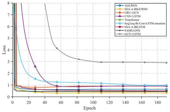
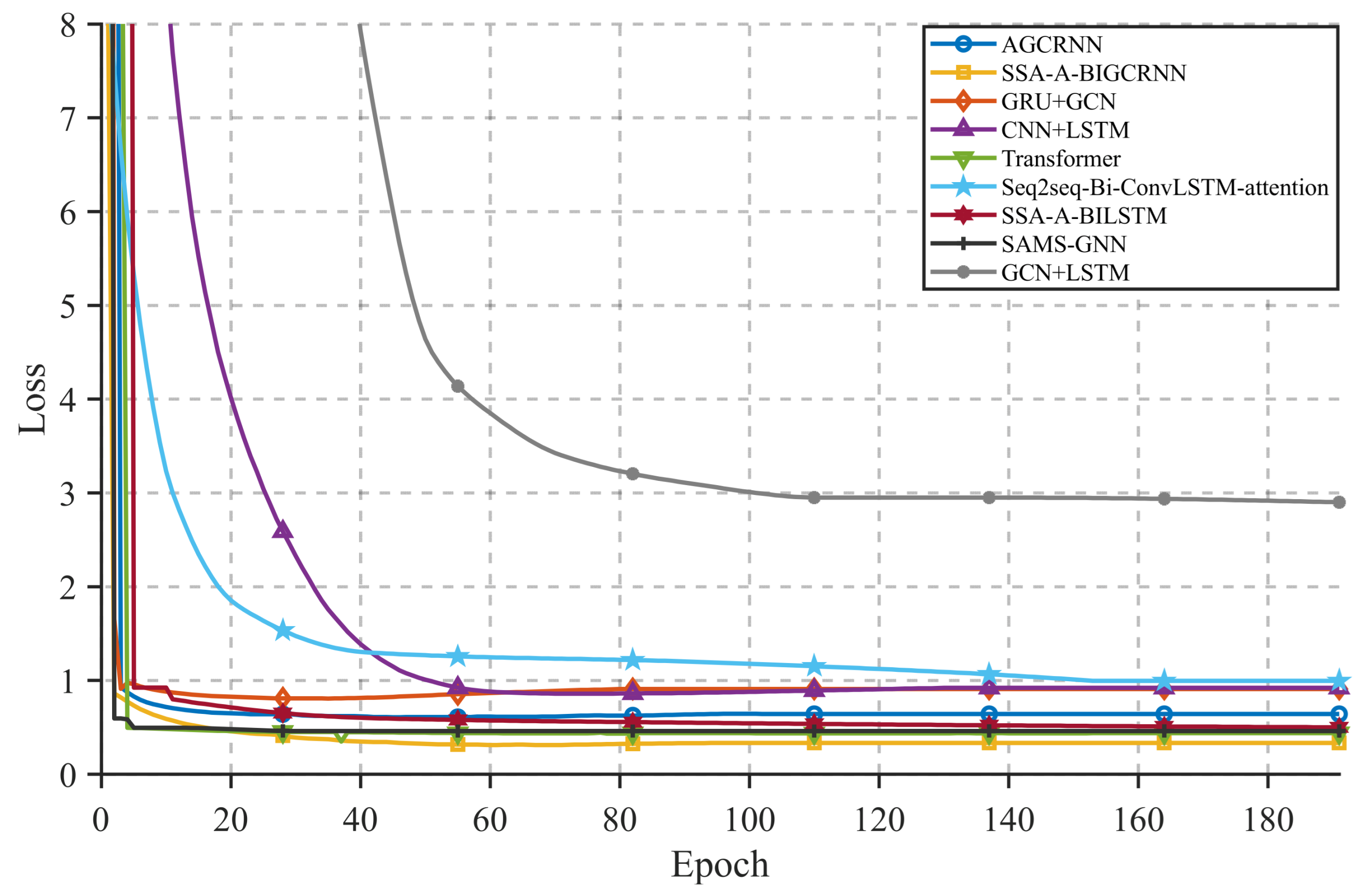
In addition to the predictive performance, we evaluated the convergence behavior of the models during the training phase. As illustrated in Figure 6, the proposed SSA-A-BiGCRNN demonstrates rapid initial convergence, with the loss dropping significantly within the first 20 epochs. Compared to baseline models such as GCN + LSTM and standard Transformer, our model not only converges faster but also achieves the lowest steady-state loss without noticeable oscillation. This indicates that the proposed attention mechanism and structural design effectively optimize the gradient descent process and enhance learning stability.

Figure 6. Training loss curves of the proposed SSA-A-BiGCRNN and baseline models over epochs.

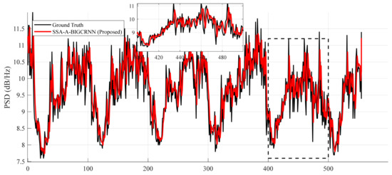
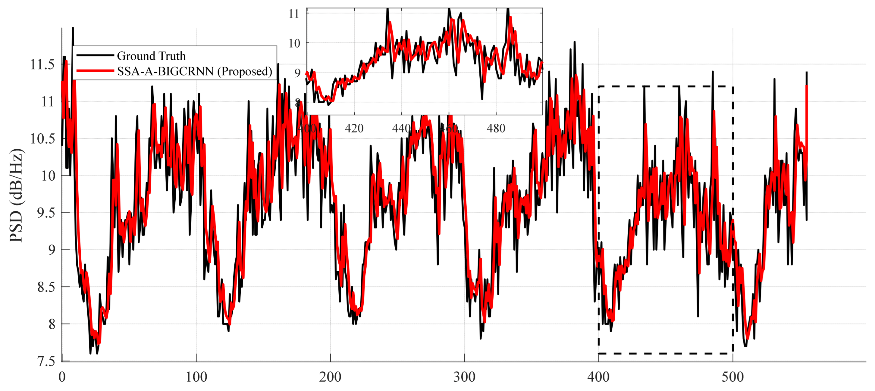
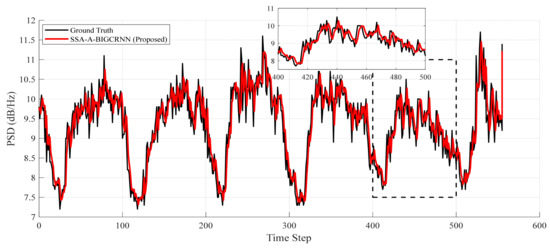
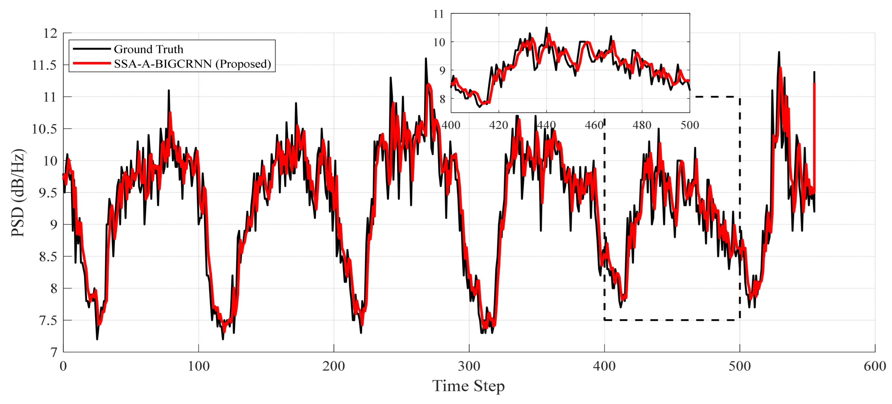
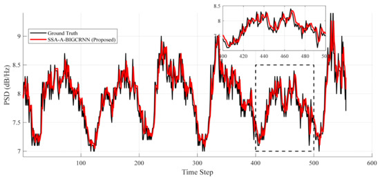
To evaluate local sequence tracking, three typical frequency bands (600–602 MHz, 702–704 MHz, and 710–712 MHz) were randomly selected. Figure 7, Figure 8 and Figure 9 compare the predicted outputs with the ground truth spectrum fluctuations.

Figure 7. Predicted spectrum results for the 600–602 MHz test set.

Figure 8. Predicted spectrum results for the 702–704 MHz test set.

Figure 9. Predicted spectrum results for the 710–712 MHz test set.

3.4. Parameter Sensitivity Analysis

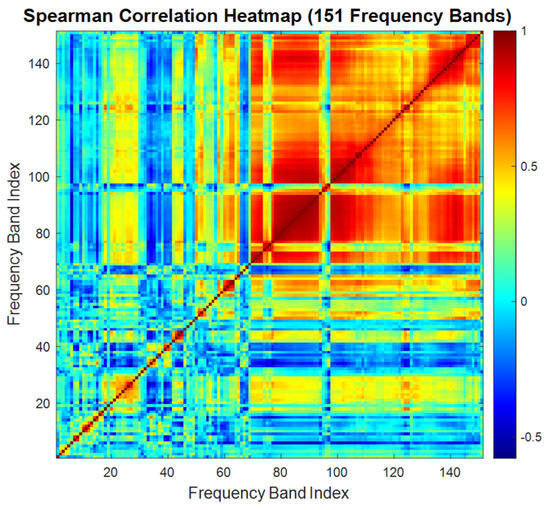
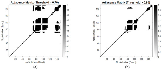
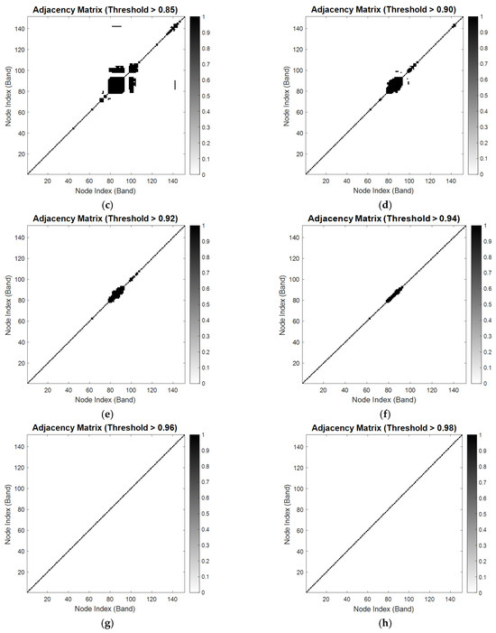
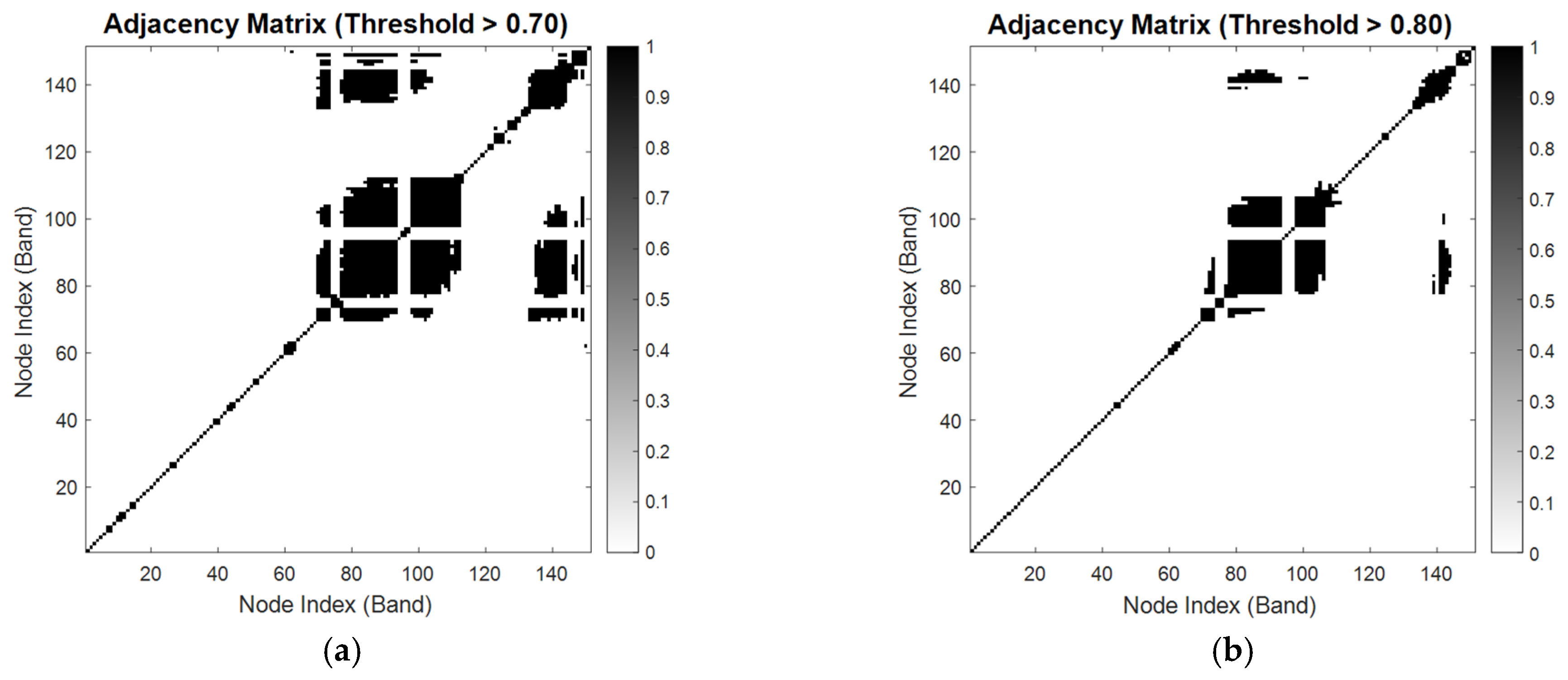
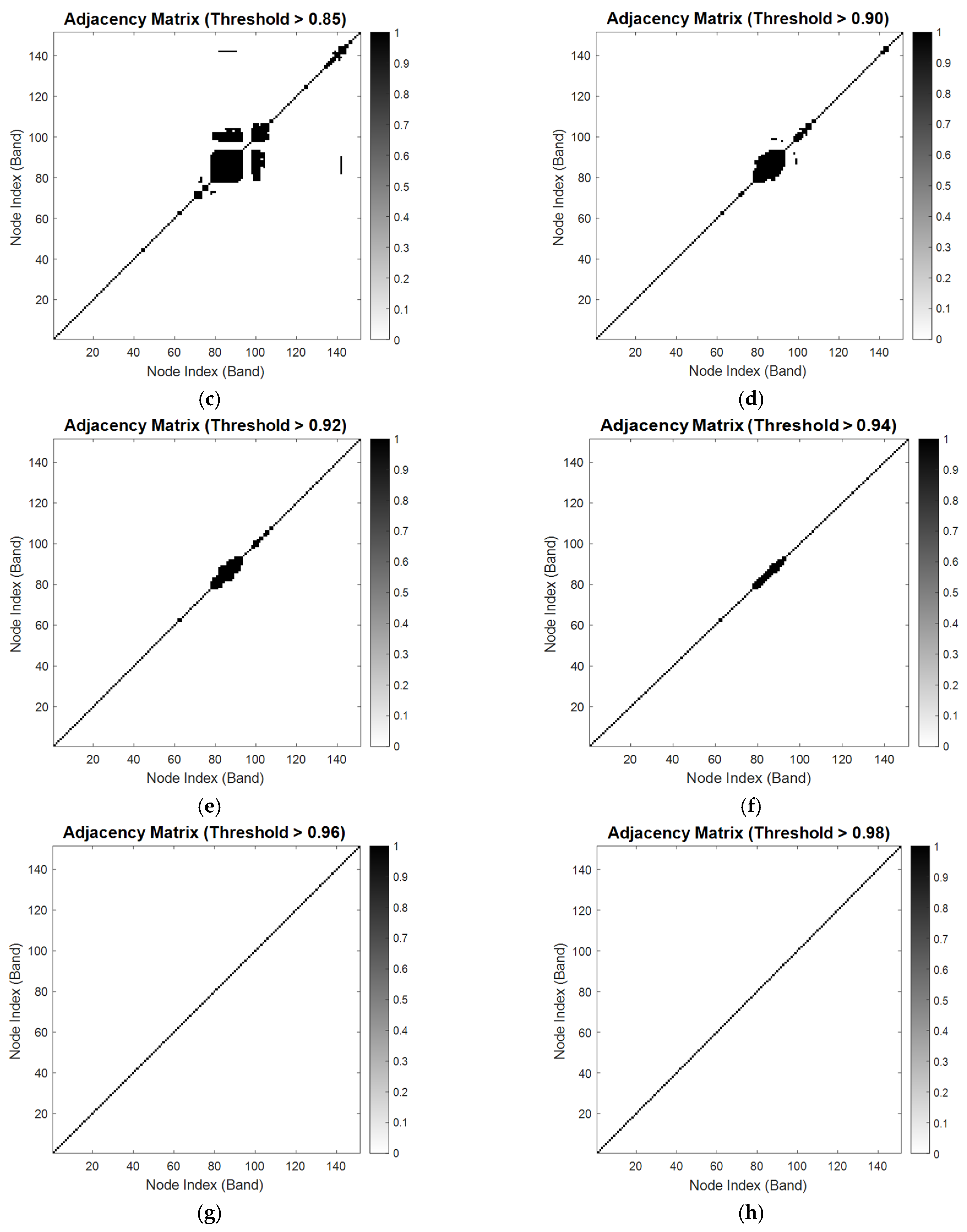
In a real electromagnetic environment, multi-band spectrum states do not evolve in isolation but exhibit complex synergistic and coupling effects. Given the lack of a prior physical topological structure among the frequency band nodes, this paper adopts a data-driven strategy. Based on historical observation sequences, the Spearman rank correlation coefficients among 151 frequency bands are calculated to quantify their joint evolutionary patterns. To prevent a fully connected dense graph from introducing background noise and triggering the over-smoothing phenomenon during feature aggregation in the GNN, a truncation mechanism is introduced. By setting a strict correlation threshold $\mathsf{\tau }$, the continuous correlation coefficient matrix is transformed into a sparse binarized adjacency matrix. The resulting frequency band correlation heatmap is shown in Figure 10, and the sparsity evolution process of the binarized adjacency matrix under different thresholds is illustrated in Figure 11.

Figure 10. Frequency band correlation heatmap.

Figure 11. Binarized adjacency matrices under different correlation thresholds: (a) 0.7; (b) 0.8; (c) 0.85; (d) 0.90; (e) 0.92; (f) 0.94; (g) 0.96; (h) 0.98.

As shown in the correlation heatmap in Figure 10, the dark areas near the main diagonal indicate that adjacent frequency bands possess a high degree of local continuity in their temporal evolution. Meanwhile, the significant correlation areas outside the diagonal region indicate that there are nonlinear long-distance coupling effects between different frequency bands. Figure 11 intuitively displays the sparsity evolution process of the adjacency matrix as the threshold $\tau$ changes, further confirming the necessity of setting a reasonable truncation threshold to filter out weakly correlated random noise.

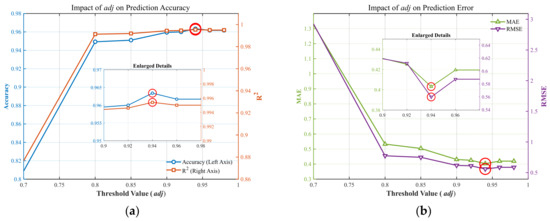
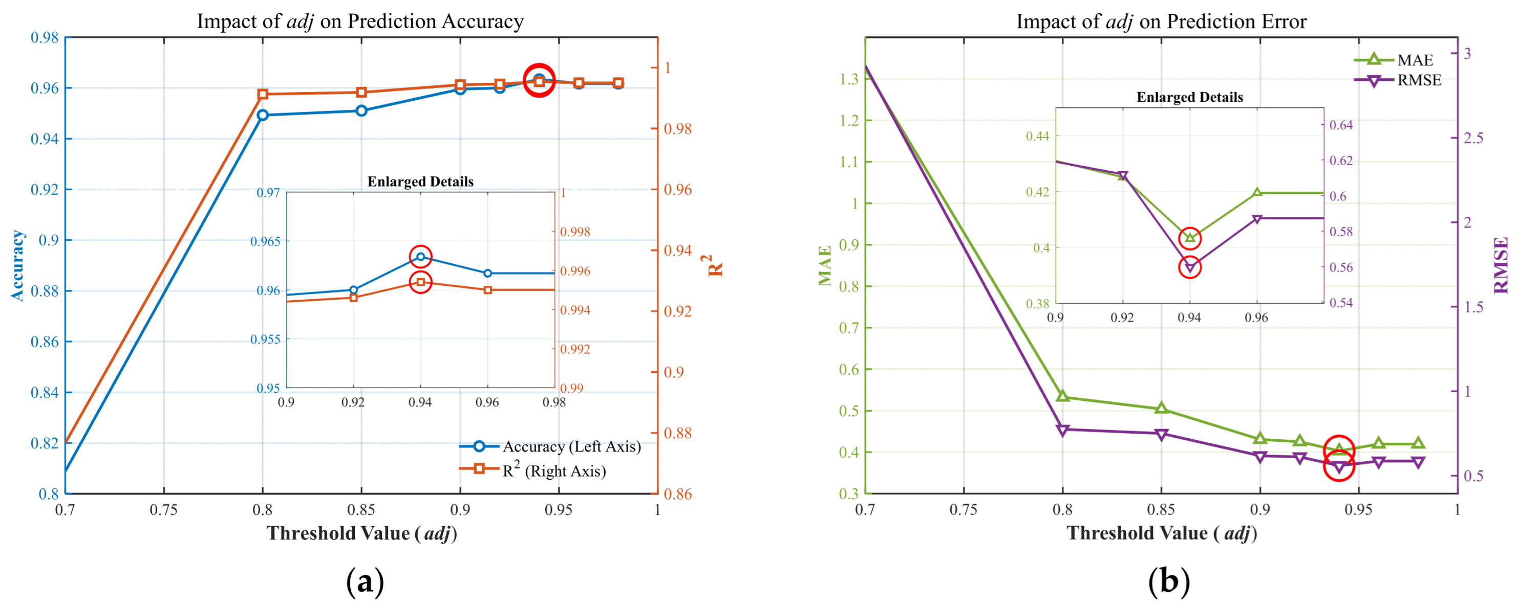
We conducted a hyperparameter sensitivity analysis to determine the optimal correlation threshold, which is crucial for balancing the bias-variance tradeoff in Graph Neural Networks. A lower $\tau$ value passively incorporates a massive amount of pseudo-correlation links triggered by random electromagnetic background noise. Theoretically, this dense topology exacerbates the “over-smoothing” phenomenon during GCN feature aggregation, causing node representations to become indistinguishable and severely degrading prediction accuracy. Conversely, an excessively high threshold leads to over-filtering, forcibly blocking cross-band harmonics and distant intermodulation interference links that possess genuine physical and mathematical correlations [16]. Therefore, the experiment performs parameter optimization for $\tau$ within the range of 0.70 to 0.98 with a step size of 0.02. The evaluation results are shown in Figure 12.

Figure 12. Effect of varying correlation thresholds on model performance: (a) Accuracy and $R^2$; (b) MAE and RMSE.

As shown in Figure 11, the prediction performance initially improves but subsequently deteriorates as the correlation threshold increases. A lower threshold creates an overly dense network topology, incorporating noise-induced pseudo-correlations that cause feature over-smoothing and higher errors. Conversely, an excessively high threshold over-filters genuine physical correlations, thereby omitting crucial spatial synergistic information and restricting the attention mechanism. The model achieves optimal comprehensive performance at a threshold of 0.94, where Accuracy and $R^2$ simultaneously peak, and MAE and RMSE drop to their minimums.

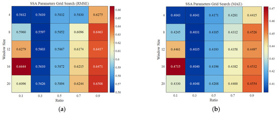
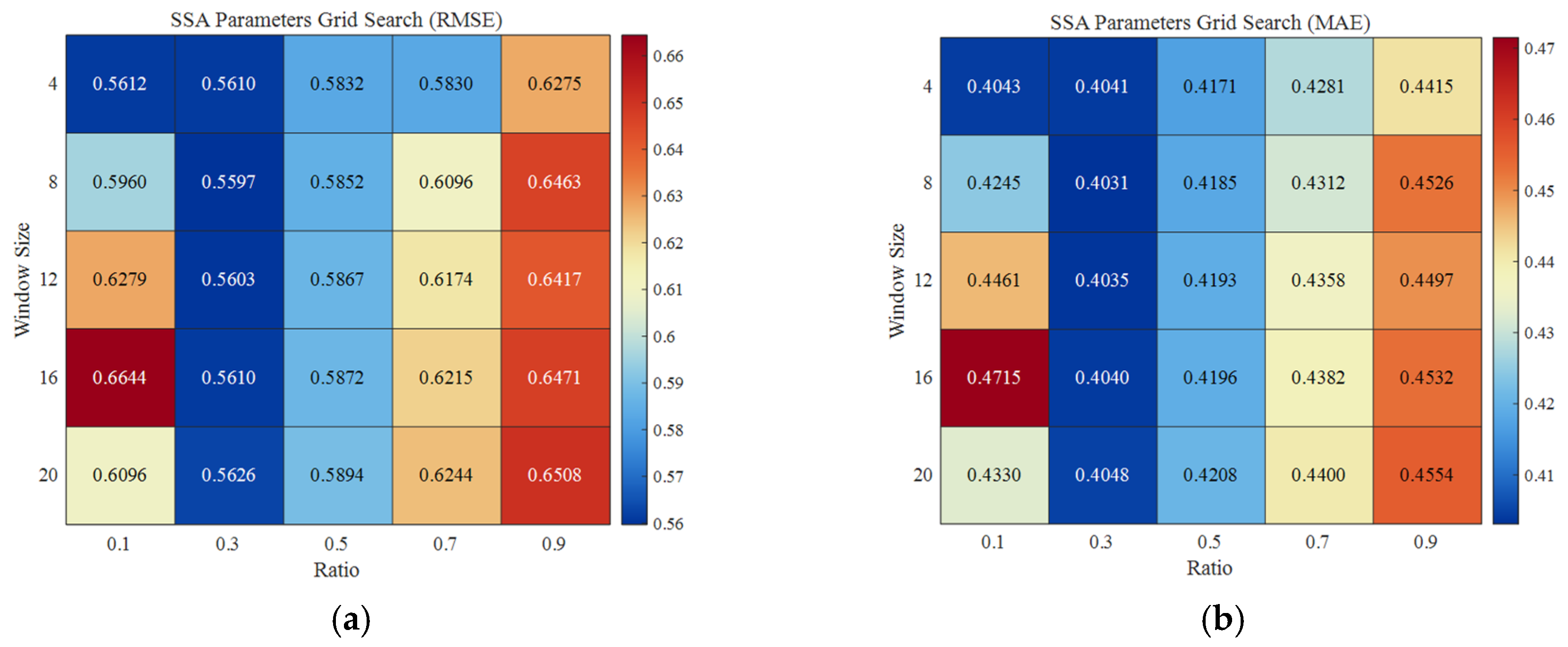
To evaluate the tuning effect of the SSA preprocessing module, we conducted a bivariate experiment on its two core hyperparameters: window length $L$ and singular value retention ratio r. L determines the analytical resolution of the signal’s multi-scale features, while r controls the trade-off between noise filtering and information preservation. We set the search interval for L to [4,20] with a step size of 4. Given the 15 min temporal resolution of our dataset, this interval spans physical observation windows of 1 to 5 h, aligning with the continuous activity cycles of typical radio services. This configuration balances feature coverage and computational efficiency. Concurrently, r was swept from 0.1 to 0.9 with a step size of 0.2 to optimize the boundary between signal and noise subspaces [22]. The experimental results are shown in Figure 13.

Figure 13. Prediction errors across different window lengths and retention ratios: (a) RMSE; (b) MAE.

Experimental results show that as L increases, both RMSE and MAE rapidly decline before leveling off. Increasing L from 4 to 12 significantly improves MAE, as the higher embedding dimension enhances the model’s ability to identify multi-scale temporal features. However, when L exceeds 16, error reduction plateaus with slight fluctuations. This indicates that an excessively large window captures local pseudo-random noise, risking over-fitting and degrading predictive capability.

The retention ratio r impacts prediction accuracy in a distinct U-shaped pattern. At $r=0.1$, the reconstructed signal suffers severe distortion due to the loss of critical spectral components, resulting in high errors. As r increases to 0.3, the model filters out approximately 70% of incoherent noise, isolating the core trend and maximizing accuracy. Conversely, increasing r beyond 0.5 reintroduces random noise during singular value reconstruction, hindering the Bi-GCRNN from extracting valid spatial correlations and causing the MAE to rebound.

Balancing robustness and real-time processing requirements, we identified $L=8$ and $r=0.3$ as the optimal parameter configuration. Under these settings, MAE and RMSE are minimized. The SSA module achieves an optimal trade-off between noise removal and feature preservation, supplying high-quality feature inputs to the downstream Bi-GCRNN and attention mechanism.

3.5. Ablation Study

We conduct an ablation study to evaluate each component’s contribution. Using a baseline GRU, we incrementally integrate SSA, GCN spatial modeling, and the attention mechanism. Table 3 lists the performance metrics.

Table 3. Numerical comparison of evaluation metrics for ablation studies.

Models	SSA	Bi	GCN	Att	MAE	RMSE	R2	Accuracy
SSA-A-BiGCRNN (Ours)	√	√	√	√	0.4031	0.5597	0.9966	0.9682
w/o SSA	×	√	√	√	0.4202	0.7437	0.9931	0.9549
w/o Attention	√	√	√	×	0.5065	0.8483	0.9907	0.9477
w/oBi-direction	√	×	√	√	0.4510	0.6357	0.9941	0.9584
w/o GCN	√	√	×	√	0.4148	0.7386	0.9932	0.9553
Base GRU	×	×	×	×	0.9418	1.7394	0.9452	0.8829

According to the quantitative results of the ablation study, the introduction of each core component generates a significant synergistic gain in model feature reconstruction and error control.

Comparing the baseline GRU with the purely time-series enhanced variant SSA-A-BiGRU (i.e., w/o GCN), the MAE achieves a precipitous drop of 55.96% (from 0.9418 to 0.4148), which preliminarily confirms the effectiveness of front-end denoising and bidirectional temporal modeling. Building upon this, after introducing GCN to capture the non-Euclidean spatial topological relationships among frequency bands, the MAE is further reduced by 2.82% (from 0.4148 to 0.4031), verifying the necessity of cross-band physical interference modeling and its effective coupling with temporal networks in breaking through the bottleneck of time-series prediction.

Furthermore, the weighting role of the attention mechanism is extremely crucial: compared to the variant lacking this mechanism (SSA-BiGCRNN, i.e., w/o Attention), the MAE of the complete model (SSA-A-BiGCRNN) drops significantly by 20.41% (from 0.5065 to 0.4031). This profoundly reveals the decisive advantage of adaptively focusing on key spatio-temporal evolutionary nodes in complex high-dimensional feature screening.

In addition, under the same spatio-temporal modeling architecture, the introduction of the front-end SSA module (i.e., comparing the complete model with the variant A-BiGCRNN, w/o SSA) reduces the MAE and RMSE by 4.07% (from 0.4202 to 0.4031) and 24.74% (from 0.7437 to 0.5597), respectively. Analyzing the underlying mechanism, this indicates that SSA effectively strips away high-frequency non-stationary background noise, greatly alleviating error accumulation and fitting difficulty during the long-range iterations of deep networks right from the data source. Consequently, this indispensable preprocessing step prevents the GCN from passively broadcasting noise across the spatial graph topology.

In summary, the proposed model achieves the global optimum across all evaluation dimensions. This fully demonstrates that the deep fusion and cascaded interaction of singular spectrum denoising and purification, bidirectional graph topological interaction, and dynamic feature weighting is the optimal paradigm for mining the complex spatio-temporal strong coupling dependencies of spectrum and achieving highly robust predictions.

4. Discussion

The experimental results in Section 3 validate that the SSA-A-BiGCRNN model effectively addresses high non-stationarity and complex non-Euclidean spatio-temporal coupling in spectrum prediction. Beyond performance metrics, the following insights elucidate the physical mechanisms and modular synergy underlying our approach.

4.1. Impact of Front-End Denoising on Spatio-Temporal Modeling

In the 500–800 MHz band, where random noise accounts for approximately 70% of raw signal variations, learning directly from raw sequences inevitably leads to error accumulation during long-range iterations—a primary limitation of existing baselines. By isolating core trends via SSA, our model prevents the downstream GCN from aggregating transient “pseudo-fluctuations.” This ensures that spatial feature extraction remains strictly focused on underlying physical evolution rather than high-frequency environmental noise.

4.2. Latent Topological Constraints in Frequency Bands

Unlike geographic networks, frequency bands lack a predefined Euclidean structure. The success of the Bi-GCRNN module confirms that spectral topology is governed by hidden physical constraints. Modeling this evolution as a non-Euclidean graph successfully captures genuine non-linear couplings. Furthermore, optimizing the correlation threshold effectively balances the network topology, preventing both noise-induced pseudo-correlations and the over-filtering of crucial spatial synergistic information.

4.3. The Synergistic Effect of the Attention Mechanism

In a heterogeneous multi-band environment, spectral states are not equally influential. The attention mechanism serves as a critical dynamic screener, adaptively weighting essential temporal nodes and spatial edges. By specifically focusing on sudden occupancy transitions that trigger cascading effects across adjacent bands, this mechanism prevents feature redundancy and significantly ensures the model’s predictive robustness.

4.4. Practical Implications and Limitations

By providing highly accurate multi-band predictions, the proposed model offers a reliable foundation for CR and Dynamic Spectrum Access, enabling secondary users to proactively avoid primary user interference and enhance overall spectrum efficiency. However, two limitations remain for future work:

Static Topology: The current Spearman-based adjacency matrix is static. For highly mobile CR networks, future research will explore dynamic graph generation to synchronize topology with real-time data.

Computational Overhead: Integrating SSA with deep GCRNNs increases computational complexity. Future studies will investigate lightweight architectures, such as Graph Transformers or knowledge distillation, to facilitate deployment on resource-constrained edge devices.

5. Conclusions

To address the highly non-stationary nature of spectrum data in real electromagnetic environments and the bottleneck problem of low prediction accuracy caused by the insufficient spatio-temporal synergistic modeling capabilities of existing models, this paper proposes an SSA-A-BiGCRNN attention-based spectrum prediction architecture oriented towards the deep synergy of spatio-temporal features.

The core contribution of this research lies in constructing an end-to-end closed loop of signal purification and spatio-temporal joint modeling. First, at the data-driven end, SSA is introduced to perform phase space reconstruction and singular value decomposition on the original complex time-series signals. This effectively strips away high-frequency non-stationary perturbations, achieving lossless reconstruction of core evolutionary trends and front-end denoising. Second, at the spatio-temporal feature extraction end, breaking through the limitations of isolated frequency band modeling, the proposed model accurately captures the cross-band coupling effects in non-Euclidean space and the bidirectional evolutionary patterns in the temporal dimension by constructing a high signal-to-noise ratio frequency band graph topology combined with Bi-GCRNN. Finally, at the network decision end, the Attention mechanism is integrated to achieve dynamic weighting and key information focusing on high-dimensional multi-scale features.

Extensive comparative and ablation experiments based on open-source real-world continuous spectrum monitoring data demonstrate that the proposed model comprehensively outperforms existing mainstream cutting-edge baseline models across core evaluation metrics such as Accuracy, MAE, and RMSE. This research not only mechanistically validates the superior accuracy and global robustness of the front-end denoising—bidirectional graph topological modeling—attention aggregation architecture on complex spectrum time-series data, but also provides a solid theoretical foundation and algorithmic basis for efficient dynamic spectrum sensing and refined management in future intelligent CR networks.

References

- Wang, C.-X.; You, X.; Gao, X.; Zhu, X.; Li, Z.; Zhang, C. On the road to 6G: Visions, requirements, key technologies, and testbeds. IEEE Commun. Surv. Tutor. 2023, 25, 905–974. [Google Scholar] [CrossRef] [Scilit]
- Acharya, P.A.K.; Singh, S.; Zheng, H. Reliable open spectrum communications through proactive spectrum access. In Proceedings of the 1st International Workshop on Technology and Policy for Accessing Spectrum; Association for Computing Machinery: New York, NY, USA, 2006; p. 5. [Google Scholar] [CrossRef] [Scilit]
- Ding, G.; Wang, J.; Wu, Q.; Yao, Y.-D.; Li, R.; Zhang, H. On the limits of predictability in real-world radio spectrum state dynamics: From entropy theory to 5G spectrum sharing. IEEE Commun. Mag. 2015, 53, 178–183. [Google Scholar] [CrossRef] [Scilit]
- Ding, G.; Jiao, Y.; Wang, J.; Zou, Y.; Wu, Q.; Yao, Y.-D. Spectrum inference in cognitive radio networks: Algorithms and applications. IEEE Commun. Surv. Tutor. 2018, 20, 150–182. [Google Scholar] [CrossRef] [Scilit]
- Wang, L.; Hu, J.; Zhang, C.; Jiang, R.; Chen, Z. Deep learning models for spectrum prediction: A review. IEEE Sens. J. 2024, 24, 28553–28575. [Google Scholar] [CrossRef] [Scilit]
- Gorcin, A.; Celebi, H.; Qaraqe, K.A.; Arslan, H. An autoregressive approach for spectrum occupancy modeling and prediction based on synchronous measurements. In Proceedings of the 2011 IEEE 22nd International Symposium on Personal, Indoor and Mobile Radio Communications, Toronto, ON, Canada, 11–14 September 2011; pp. 705–709. [Google Scholar] [CrossRef] [Scilit]
- Eltom, H.; Kandeepan, S.; Liang, Y.-C.; Evans, R.J. Cooperative soft fusion for HMM-based spectrum occupancy prediction. IEEE Commun. Lett. 2018, 22, 2144–2147. [Google Scholar] [CrossRef] [Scilit]
- Wang, Y.; Zhang, Z.; Ma, L.; Chen, J. SVM-based spectrum mobility prediction scheme in mobile cognitive radio networks. Sci. World J. 2014, 2014, 395212. [Google Scholar] [CrossRef] [Scilit]
- Soni, B.; Patel, D.K.; López-Benítez, M. Long short-term memory based spectrum sensing scheme for cognitive radio using primary activity statistics. IEEE Access 2020, 8, 97437–97451. [Google Scholar] [CrossRef] [Scilit]
- Tusha, A.; Kaplan, B.; Cırpan, H.A.; Qaraqe, K.; Arslan, H. Intelligent spectrum occupancy prediction for realistic measurements: GRU based approach. In Proceedings of the 2022 IEEE International Black Sea Conference on Communications and Networking (BlackSeaCom), Sofia, Bulgaria, 6–9 June 2022; pp. 179–184. [Google Scholar] [CrossRef] [Scilit]
- Wang, X.; Chen, Q.; Yu, X. Research on spectrum prediction technology based on B-LTF. Electronics 2023, 12, 247. [Google Scholar] [CrossRef] [Scilit]
- Zhang, X.; Yu, G.; Cui, Y.; Shang, J. Short-term traffic flow prediction based on clustering algorithm and Graph neural network. J. Jilin Univ. (Eng. Technol. Ed.) 2024, 54, 1593–1600. [Google Scholar]
- Shawel, B.S.; Woldegebreal, D.H.; Pollin, S. Convolutional LSTM-based long-term spectrum prediction for dynamic spectrum access. In Proceedings of the 2019 27th European Signal Processing Conference (EUSIPCO), A Coruña, Spain, 2–6 September 2019; pp. 1–5. [Google Scholar] [CrossRef] [Scilit]
- Ding, X.; Feng, L.; Zou, Y.; Zhang, G. Deep learning aided spectrum prediction for satellite communication systems. IEEE Trans. Veh. Technol. 2020, 69, 16314–16319. [Google Scholar] [CrossRef] [Scilit]
- Ren, X.; Mosavat-Jahromi, H.; Cai, L.; Kidston, D. Spatio-temporal spectrum load prediction using convolutional neural network and ResNet. IEEE Trans. Cogn. Commun. Netw. 2021, 8, 502–513. [Google Scholar] [CrossRef] [Scilit]
- Zhang, X.; Guo, L.; Ben, C.; Peng, Y.; Shi, S. A-GCRNN: Attention graph convolution recurrent neural network for multi-band spectrum prediction. IEEE Trans. Veh. Technol. 2024, 73, 2978–2982. [Google Scholar] [CrossRef] [Scilit]
- Zhang, X.; Peng, Y.; Huang, H.; Wang, Y.; Wang, Q.; Lin, Y.; Qin, Z.; Gui, G. SAMS-GNN: Self-adaptive multi-scale graph neural network for multi-band spectrum prediction. IEEE Trans. Cogn. Commun. Netw. 2025, 11, 1442–1451. [Google Scholar] [CrossRef] [Scilit]
- Vaswani, A.; Shazeer, N.; Parmar, N.; Uszkoreit, J.; Jones, L.; Gomez, A.N.; Kaiser, Ł.; Polosukhin, I. Attention is all you need. In Proceedings of the 31st Conference on Neural Information Processing Systems (NeurIPS), Long Beach, CA, USA, 4–9 December 2017; pp. 1–15. [Google Scholar]
- Rabiu, E.O.; Akande, D.O.; Adeyemo, Z.K.; Akanbi, I.A.; Obanisola, O.O. Three-state hidden Markov model for spectrum prediction in cognitive radio networks. ABUAD J. Eng. Res. Dev. 2024, 7, 425–435. [Google Scholar] [CrossRef] [Scilit]
- Wang, W.-C.; Ye, F.-R.; Wang, Y.-Y.; Gu, M. A singular spectrum analysis-enhanced BiTCN-self-attention model for runoff prediction. Earth Sci. Inform. 2025, 18, 31. [Google Scholar] [CrossRef] [Scilit]
- Pan, G.; Li, J.; Li, M. Multi-channel multi-step spectrum prediction using transformer and stacked Bi-LSTM. China Commun. 2025, 22, 1–13. [Google Scholar] [CrossRef] [Scilit]
- Ben, C.; Peng, Y.; Wang, Y.; Zhang, Q.; Guo, L.; Lin, Y. Enhanced multi-band spectrum prediction using singular spectrum analysis and attention-based BiLSTM. IEEE Trans. Cogn. Commun. Netw. 2024, 11, 118–126. [Google Scholar] [CrossRef] [Scilit]
- Guo, N.; Zhang, J.; Jiang, X. Spectrum prediction method based on time-frequency fusion attention network. J. Chongqing Univ. Posts Telecommun. (Nat. Sci. Ed.) 2025, 37, 305–314. [Google Scholar] [CrossRef]
- Chen, T.; Gao, S.; Zheng, S.; Yu, S.; Xuan, Q.; Lou, C. EMD and VMD empowered deep learning for radio modulation recognition. IEEE Trans. Cogn. Commun. Netw. 2023, 9, 43–57. [Google Scholar] [CrossRef] [Scilit]
- Li, R.; Liu, C.; Wang, S.; Lin, Y.; Gui, G. Lightweight continuous-time graph learning for spectrum prediction in 6G networks. IEEE Internet Things J. 2026; in press. [CrossRef] [Scilit]
- Yang, Q.; Deng, C.; Chang, X. Ultra-short-term/short-term wind speed prediction based on improved singular spectrum analysis. Renew. Energy 2022, 184, 36–44. [Google Scholar] [CrossRef] [Scilit]
- Shao, Z.; Han, J.; Zhao, W.; Zhou, K.; Yang, S. A novel hybrid model for short-term wind power prediction based on combined singular spectrum analysis and recurrent neural network. Energy Convers. Manag. 2022, 270, 116138. [Google Scholar] [CrossRef] [Scilit]
- Ta, X.; Liu, Z.; Hu, X.; Yu, L.; Sun, L.; Du, B. Adaptive spatio-temporal graph neural network for traffic forecasting. Knowl. Based Syst. 2022, 242, 108199. [Google Scholar] [CrossRef] [Scilit]
- Yoon, C.; Yim, S.; Yoo, S.; Jung, C.; Yeon, H.; Jang, Y. V-DCRNN: Virtual network-based diffusion convolutional recurrent neural network for estimating unobserved traffic data. IEEE Trans. Intell. Transp. Syst. 2025, 26, 10336–10352. [Google Scholar] [CrossRef] [Scilit]
- Rajendran, S.; Calvo-Palomino, R.; Fuchs, M.; Van den Bergh, B.; Cordobes, H.; Giustiniano, D. ElectroSense: Open and big spectrum data. IEEE Commun. Mag. 2018, 56, 210–217. [Google Scholar] [CrossRef] [Scilit]
- Riihijärvi, J. Empirical Modelling of Spectrum Use and Evaluation of Adaptive Spectrum Sensing in Dynamic Spectrum Access Networks. Ph.D. Thesis, RWTH Aachen University, Aachen, Germany, 2010. [Google Scholar]
- Wang, L.; Hu, J.; Jiang, R.; Chen, Z. A deep long-term joint temporal–spectral network for spectrum prediction. Sensors 2024, 24, 1498. [Google Scholar] [CrossRef] [Scilit]
- Zhang, H.; Tian, Q.; Han, Y. Multi channel spectrum prediction algorithm based on gcn and lstm. In Proceedings of the 2022 IEEE 96th Vehicular Technology Conference (VTC2022-Fall), London, UK, 26–29 September 2022; pp. 1–5. [Google Scholar] [CrossRef] [Scilit]
- Chen, W.; Zhai, C.; Wang, X.; Li, J.; Lv, P.; Liu, C. GCN- and GRU-based intelligent model for temperature prediction of local heating surfaces. IEEE Trans. Ind. Inform. 2022, 19, 5517–5529. [Google Scholar] [CrossRef] [Scilit]
Disclaimer/Publisher’s Note: The statements, opinions and data contained in all publications are solely those of the individual author(s) and contributor(s) and not of MDPI and/or the editor(s). MDPI and/or the editor(s) disclaim responsibility for any injury to people or property resulting from any ideas, methods, instructions or products referred to in the content. |
© 2026 by the authors. Licensee MDPI, Basel, Switzerland. This article is an open access article distributed under the terms and conditions of the Creative Commons Attribution (CC BY) license.