


Abstract
Dynamic atomic force microscopy (AFM) is a key technique for nanoscale characterization and mechanical property measurement, where the geometric shape of the probe tip critically determines imaging quality and measurement accuracy. This study proposes a tip shape classification framework based on the dynamic response of the AFM microcantilever. First, a dimensionless dynamic model of the microcantilever is established, and its vibrational response is solved using a finite-difference scheme. For conical, spherical, and flat tip geometries, interaction force models are provided under both non-contact and tapping-mode AFM. Based on these formulations, multidimensional dynamic feature parameters, including amplitude, phase, virial, and root-mean-square force, are extracted. On this basis, an XGBoost-based classifier is constructed for tip shape identification, and the model’s decision-making mechanism is further interpreted through a SHAP-based explainability framework combined with dimensionality reduction and visualization techniques. Results show that, under non-contact conditions, the overall classification accuracy on the test set reaches 96.7%, with a 100% recognition rate for conical tips. Under tapping-mode conditions, the classification accuracies for conical, spherical, and flat tips are 100%, 85.5%, and 98.3%, respectively. The results demonstrate the feasibility of identifying tip shapes from dynamic responses using simulated data, thereby establishing a theoretical and methodological basis for future experimental validation and the development of tip diagnostic techniques.
1. Introduction
Atomic force microscopy (AFM) is a core tool for nanoscale mechanical measurement and surface morphology characterization. The probe, as a key component of AFM imaging, consists of a microcantilever and a tip located at its free end. During imaging, interaction forces between the tip and the sample induce deformation of the microcantilever or changes in its dynamic state. The feedback system reconstructs the three-dimensional surface morphology by maintaining a constant tip–sample interaction force [1]. Dynamic AFM is widely used due to its minimal sample damage and broad applicability across different materials. The geometric shape of the probe tip directly determines imaging resolution and measurement accuracy. However, during dynamic AFM operation, including non-contact and tapping modes, the tip inevitably undergoes wear, blunting, or fracture. These effects lead to tip–sample convolution, which consequently introduces imaging artifacts, significantly affecting the accuracy and reproducibility of quantitative measurements. Therefore, the development of tip shape identification methods is crucial for enhancing AFM imaging fidelity.
Substantial research has been devoted to monitoring tip wear and characterizing tip morphology. Kopycinska et al. [2,3] investigated the contact mechanics of the tip–sample interaction, finding that the actual contact behavior cannot be accurately described by simple idealized geometries. Killgore et al. [4] proposed an indirect approach for evaluating probe tip wear by monitoring shifts in the contact resonance frequency of the microcantilever. Liu et al. [5] combined adhesion force measurements with intermittent transmission electron microscopy (TEM) characterization to assess tip properties during contact-mode scanning. Li et al. [6] identified two distinct tip wear stages: an initial rapid wear stage followed by a gradual steady-state wear stage. Huang et al. [7] investigated the wear behavior of single-crystal silicon probes during nanofabrication processes, enabling rapid detection of tip wear and classification of wear stages. For tip shape reconstruction, VanLandingham et al. [8] employed mathematical morphology algorithms to perform three-dimensional analysis of different tip geometries from AFM images. Nguyen and Chung [9] demonstrated that tip shape significantly influences the tip–sample interactions through indentation data obtained with different tip geometries. However, most of these approaches rely on specialized imaging equipment or involve complex mechanical inverse analyses. Moreover, limited attention has been paid to the direct relationship between tip geometry and the dynamic response of the probe, which constitutes the fundamental physical basis for online identification.
Based on wear progression, the probe tip can be simplified into three representative geometries, namely conical, spherical, and flat configurations [10,11]. Tip–sample interaction forces differ fundamentally for each geometry, directly modulating dynamic response characteristics of the cantilever, including oscillation amplitude, phase, virial, and root-mean-square force (FRMS). Accordingly, the problem of tip shape classification can be essentially reformulated as a pattern recognition problem based on dynamic responses. Machine learning methods have recently been introduced to address the identification of tip–sample interaction forces. Yu et al. [12] proposed a cross-scale ML-PSP-AM framework, summarized machine learning applications in laser metal additive manufacturing and analyzed corresponding research bottlenecks, alongside four future development paths. Elsherbiny et al. [13] employed various machine learning algorithms to predict interaction forces of different power-law forms based on dynamic response signals. Matsunaga et al. [14] proposed an end-to-end deep learning approach for tip reconstruction, which exhibits strong robustness against noise in AFM images. However, most existing studies have primarily focused on the inverse identification of tip–sample interaction force model parameters or post-processing of imaging data. A systematic framework for tip shape classification based on probe dynamic responses has not yet been established, and limited attention has been paid to the interpretability of the classification models.
The eXtreme Gradient Boosting (XGBoost) is an efficient gradient-boosted decision tree algorithm that has been widely adopted owing to its superior predictive performance, robustness, and strong capability in handling high-dimensional features and complex nonlinear relationships [15,16]. Recent studies have demonstrated the effectiveness of XGBoost in engineering applications, particularly when combined with SHapley Additive exPlanations (SHAP) analysis for model interpretability [12,17,18]. These developments provide a solid methodological foundation for integrating tree-based ensemble learning with physical interpretability in complex engineering classification tasks. In this study, a framework for tip shape classification based on the dynamic response of an AFM probe is proposed. First, a dimensionless dynamic model of the microcantilever is established, and its vibrational response is solved using a finite-difference method, thereby decoupling physical parameters and enhancing both computational efficiency and general applicability. Interaction force models are then developed for three representative tip geometries, conical, spherical, and flat, under both non-contact and tapping-mode conditions. Based on these models, multidimensional dynamic features, including oscillation amplitude, phase, virial, and FRMS, are systematically extracted. Furthermore, an XGBoost-based classifier is constructed for tip shape identification, and the decision-making process is interpreted using SHAP analysis combined with dimensionality reduction and visualization techniques, thereby revealing the key physical features that dominate classification performance [17,18]. It should be noted that the present study is based on idealized models and simulated data. The three representative geometries can be regarded as simplified representations of realistic tip wear processes: the conical shape approximates a sharp tip, the spherical shape corresponds to a nanoscale blunted apex, and the flat shape represents a severely worn or fractured tip end. Such simplification facilitates the clarification of the constitutive mapping relationship between probe dynamic responses and tip geometry. Unlike previous machine-learning-assisted AFM studies that mainly focus on image-based analysis or mechanical property prediction, the proposed framework establishes a physics-guided workflow for tip shape identification based on dynamic response signals. Rather than relying on raw measurement data, four physically meaningful features (amplitude, phase, virial, and FRMS) are extracted from the AFM dynamic model and integrated with an interpretable machine learning framework consisting of XGBoost and SHAP analysis.
2. AFM Microcantilever Dynamic Model and Numerical Solution
2.1. Governing Equation and Boundary Conditions
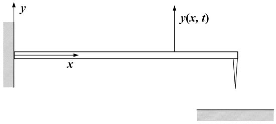
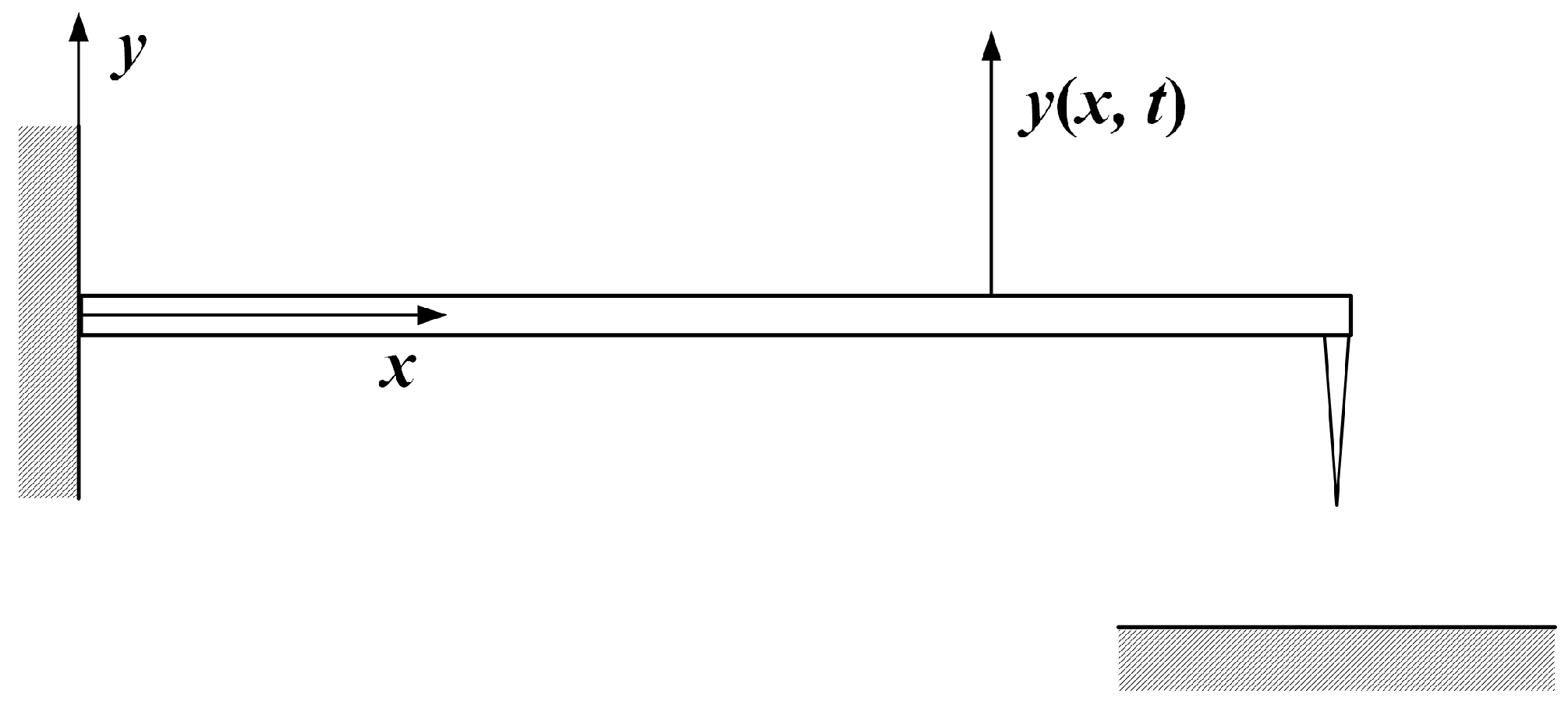
The dynamic mechanical behavior of the AFM microcantilever is described by the Euler–Bernoulli beam model, as illustrated in Figure 1. The governing differential equation of its vibration is given as follows:
where y(x,t) denotes the deflection of the microcantilever at time t and position x measured from the fixed end; E is the Young’s modulus of the microcantilever; I is the area moment of inertia of the cross-section; ρ is the density of the microcantilever; A is the cross-sectional area; and κ represents the air damping coefficient.
Figure 1.
Schematic diagram of the microcantilever model in dynamic AFM.
At the fixed end (x = 0), a sinusoidal displacement excitation is applied, while the free end is subjected to the tip–sample interaction force Fts. The corresponding boundary conditions are given as follows:
where u0 is the amplitude of the excitation displacement, ωexc is the angular excitation frequency, and d denotes the instantaneous tip–sample separation distance.
2.2. Non-Dimensionalization
To mitigate parameter coupling, improve numerical stability, and enhance the generality of the dimensional governing equations, characteristic length and characteristic time scales are introduced for non-dimensionalization. The following dimensionless variables are defined:
where L is the length of the microcantilever and ω0 is the fundamental natural frequency of the first vibration mode. Substituting Equation (3) into Equation (1), the governing equation can be reformulated in a dimensionless form as follows:
It can be observed that the five physical parameters in the original governing equation (E, I, ρ, A, κ) are condensed into two dimensionless parameters (ζa, λ), thereby significantly reducing the dimensionality of the parameter space. The corresponding dimensionless boundary conditions are given as follows:
In the above expression, the frequency ratio β and the dimensionless tip–sample interaction force are defined as follows:
2.3. Finite Difference Numerical Solution
The dimensionless governing equation is discretized using the finite difference method. The spatial domain [0, 1] is divided into n equal intervals with a nodal spacing of Δξ = 1/n, and the time step is Δτ. The fourth-order spatial derivative is approximated using a five-point central difference scheme, while the second-order time derivative uses a central difference scheme, and the first-order time derivative uses a forward difference scheme. The initial conditions are assumed to be a quiescent state. The displacements of the boundary nodes are determined using boundary conditions via the virtual node method. By arranging the nodal displacements in spatial order into a vector form, the following explicit iterative scheme can be obtained:
where Yj is the displacement vector at the j-th time step,
is an n × n coefficient matrix, and G is the source vector incorporating both the excitation and the tip–sample interaction force. Their expressions are given as follows:
C and D are dimensionless constants, whose expressions are given as follows:
3. Tip Shape Classification in Non-Contact Mode
3.1. Dynamic Model and Response Analysis in Non-Contact Mode
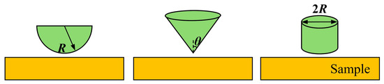
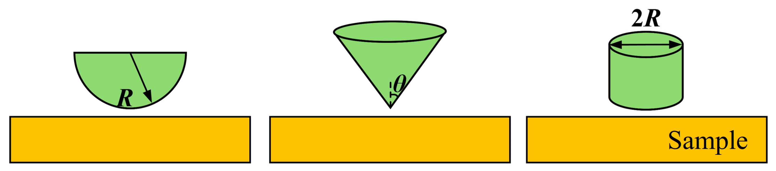
Three representative tip geometries, i.e., spherical, conical, and flat, are considered as illustrated in Figure 2. The interaction forces between the tip and the sample differ fundamentally for each geometry, directly modulating the dynamic response of the microcantilever. Therefore, the tip geometry can be inferred by analyzing the dynamic response of the microcantilever.
Figure 2.
Schematic diagrams of three tip shapes in non-contact mode.
In non-contact mode, the tip–sample interaction force is governed by van der Waals attractive forces [19,20]. The dimensional van der Waals force is defined and subsequently non-dimensionalized by substituting into Equation (6). For a spherical tip, this interaction is:
where H is the Hamaker constant, R is the tip radius, d is the instantaneous tip–sample distance, and a0 is the intermolecular distance. For a conical tip, the van der Waals force is:
where θ is the half-opening angle of the conical tip. For a flat tip, the van der Waals interaction force is expressed as follows:
In addition to the dimensionless amplitude and phase of the microcantilever, dimensionless virial and FRMS are also introduced as dynamic response features [1,21,22]:
where Ytip denotes the dimensionless displacement at the free end of the microcantilever.
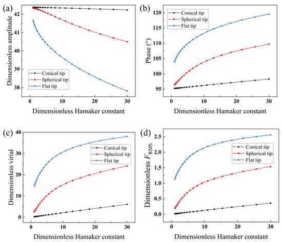
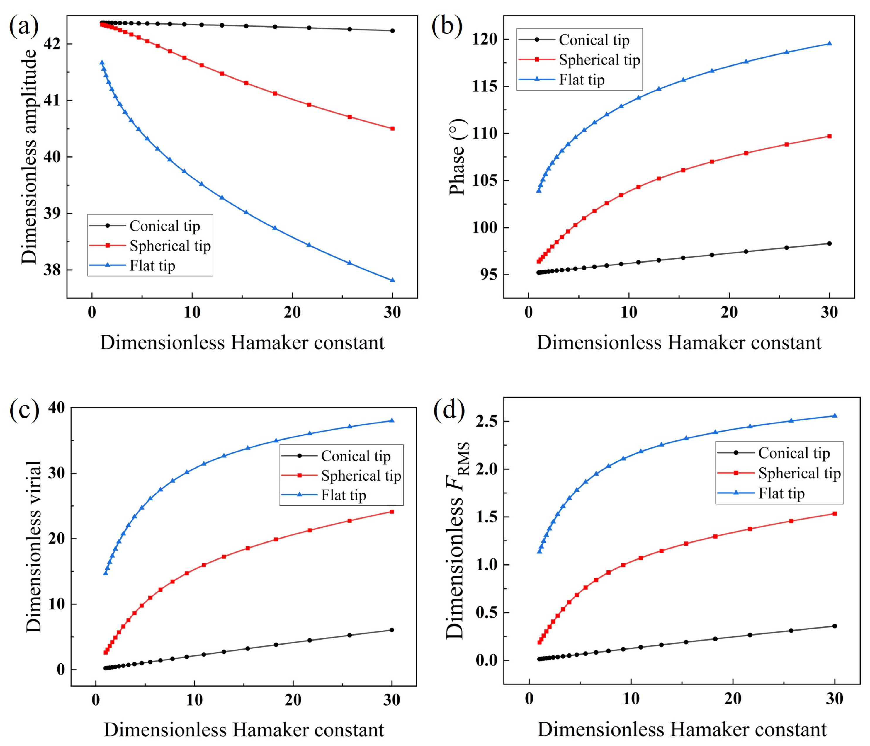
A sinusoidal displacement excitation is applied at the fixed end of the microcantilever, and the dynamic response in the non-contact mode is solved. The geometric and mechanical parameters of the probe are listed in Table 1, yielding dimensionless parameters ζa = 0.455, λ = 3.519. At excitation frequency ratio β = 1, the dimensionless free amplitude is 42.38. To maintain purely attractive interaction, the dimensionless microcantilever-sample separation is set to 44. A reference van der Waals interaction energy scale H0 = 10−20 J is introduced, with a dimensionless Hamaker constant defined as . To simulate different surface material properties, the Hamaker constant is treated as a variable, and 200 values are selected within the range of 1~30 × 10−20 J following a logarithmic distribution. The in-phase and quadrature method is employed to compute the dimensionless amplitude, phase, virial, and FRMS for the three tip geometries. The results are shown in Figure 3.
Table 1.
Dimensions and mechanical parameters of the microcantilever.
Figure 3.
Dynamic response of the microcantilever as a function of Hamaker constant for three tip shapes in non-contact mode: (a) dimensionless amplitude, (b) phase, (c) dimensionless virial, (d) dimensionless FRMS.
As shown in Figure 3a, with increasing Hamaker constant, the spherical and flat tips, owing to their relatively larger effective interaction areas, exhibit greater suppression of vibration, leading to more rapid amplitude attenuation. In contrast, the conical tip’s strong spatial localization at its apex limits the effective interaction area, resulting in weak attractive force modulation and nearly constant amplitude. In Figure 3b, the flat tip experiences the steepest force-field gradient, producing the most rapid phase increase with Hamaker constant; the spherical tip follows, while the conical tip exhibits the most gradual phase variation. The virial, reflecting the integrated interaction force over one oscillation cycle, increases sharply for the flat tip with dimensionless Hamaker constant (Figure 3c), followed by the spherical tip, while the conical tip remains almost unchanged. The evolution of the dimensionless FRMS (Figure 3d) is consistent with that of the virial. Overall, the dynamic responses of the conical tip are least sensitive to variations in the dimensionless Hamaker constant, whereas the flat and spherical tips exhibit pronounced dependencies, providing a clear physical basis for tip shape classification.
3.2. XGBoost-Based Classification Model and Interpretability Analysis in Non-Contact Mode
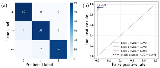
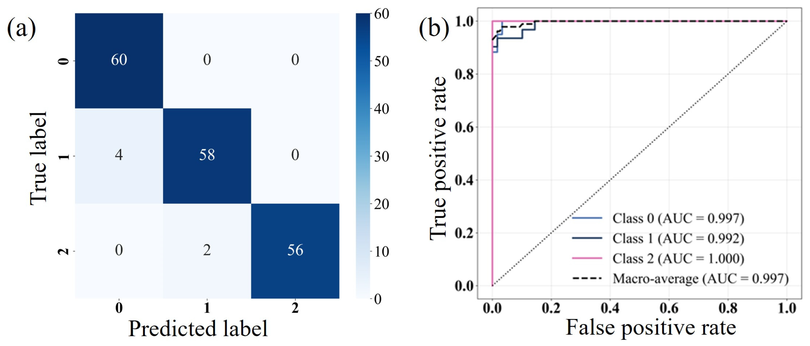
The dynamic response data for the three tip geometries are integrated, with conical, spherical, and flat tips labeled as 0, 1, and 2, respectively. After mixing, the samples are randomly shuffled and divided into training and test sets with a ratio of 7:3. An XGBoost classifier is constructed with four dynamic features as input and tip category as output. The model uses 300 decision trees with constrained maximum depth and random subsampling to mitigate overfitting and enhance generalization. The results show that the overall accuracy on the training set reaches 100%. On the test set, the overall accuracy is 96.7%, with classification accuracies of 100% for conical tips, 93.6% for spherical tips, and 96.6% for flat tips. As shown in the confusion matrix in Figure 4a, the numbers of test samples for conical, spherical, and flat tips are 60, 62, and 58, respectively. Among them, four spherical samples are misclassified as conical, and two flat samples are misclassified as spherical. The ROC curves in Figure 4b yield AUC values of 0.997 (spherical), 0.992 (conical), and 1.000 (flat), all near unity, indicating strong class separability capability of the model. Misclassifications primarily occur between spherical and conical tips, and between flat and spherical tips, suggesting that the feature space of spherical tip partially overlaps with both extremes, while no direct misclassification occurs between conical and flat tips.
Figure 4.
(a) Confusion matrix and (b) ROC curves for tip shape classification in non-contact mode.
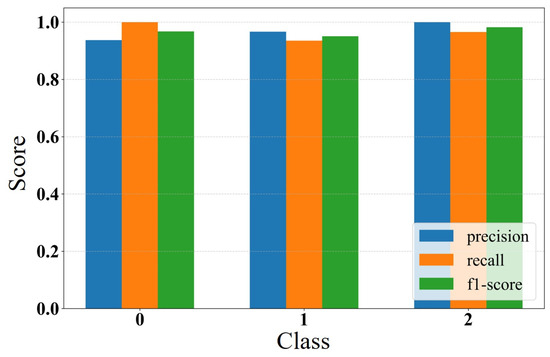
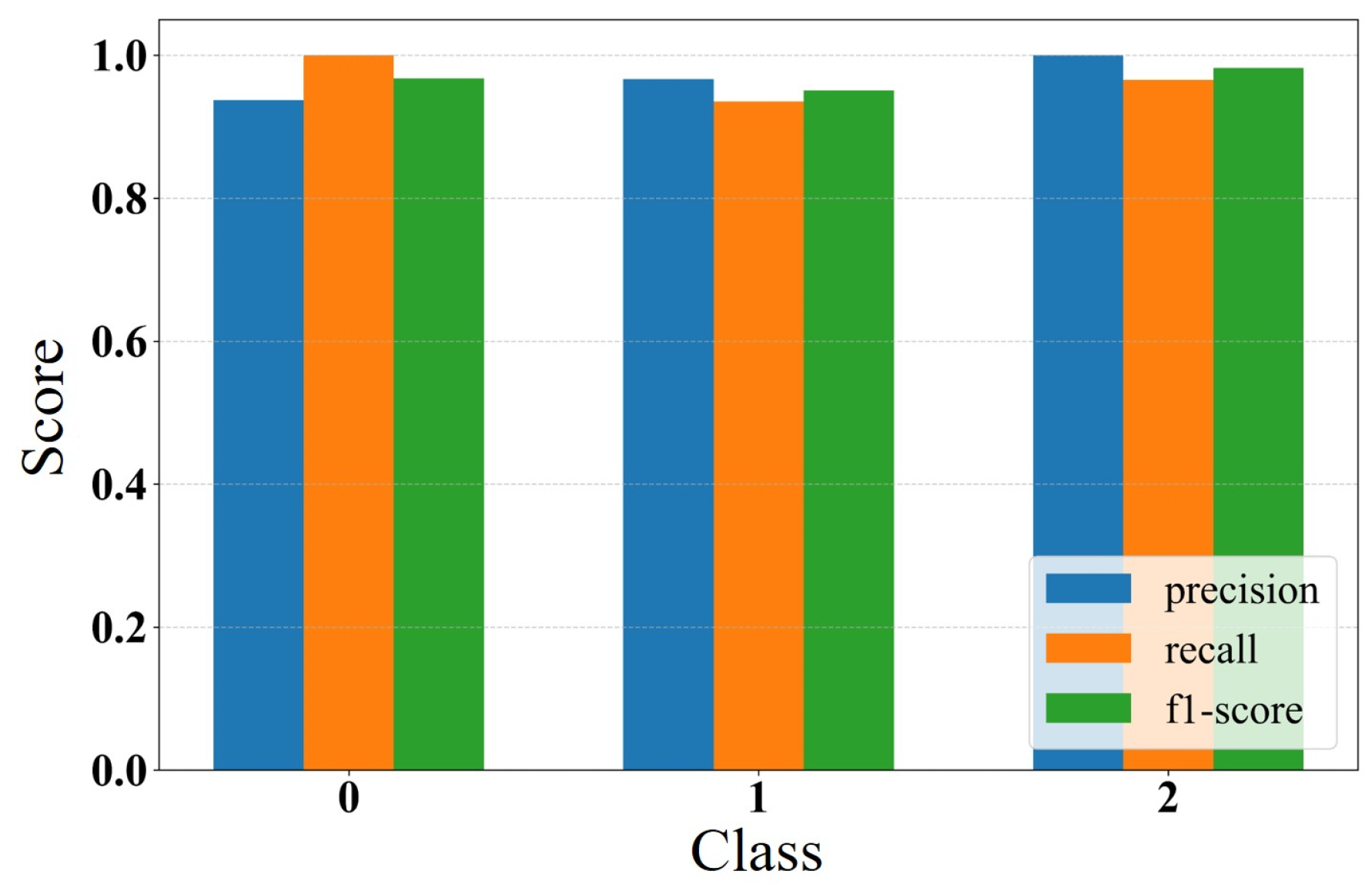
Precision, recall, and F1-score are further evaluated in Figure 5. For conical and flat tips, all three metrics are close to 1.0. For the spherical tip, the recall (0.936) is slightly lower than precision (0.967), yielding an F1-score of 0.951, indicating limited misclassifications primarily assigned to the conical category. This suggests partial dynamic feature similarity between spherical and conical tips, causing locally blurred decision boundaries in the feature space. Nevertheless, precision for all three tip geometries exceeds 0.96, demonstrating high prediction reliability.
Figure 5.
Bar chart of classification performance metrics in non-contact mode.
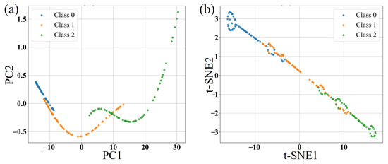
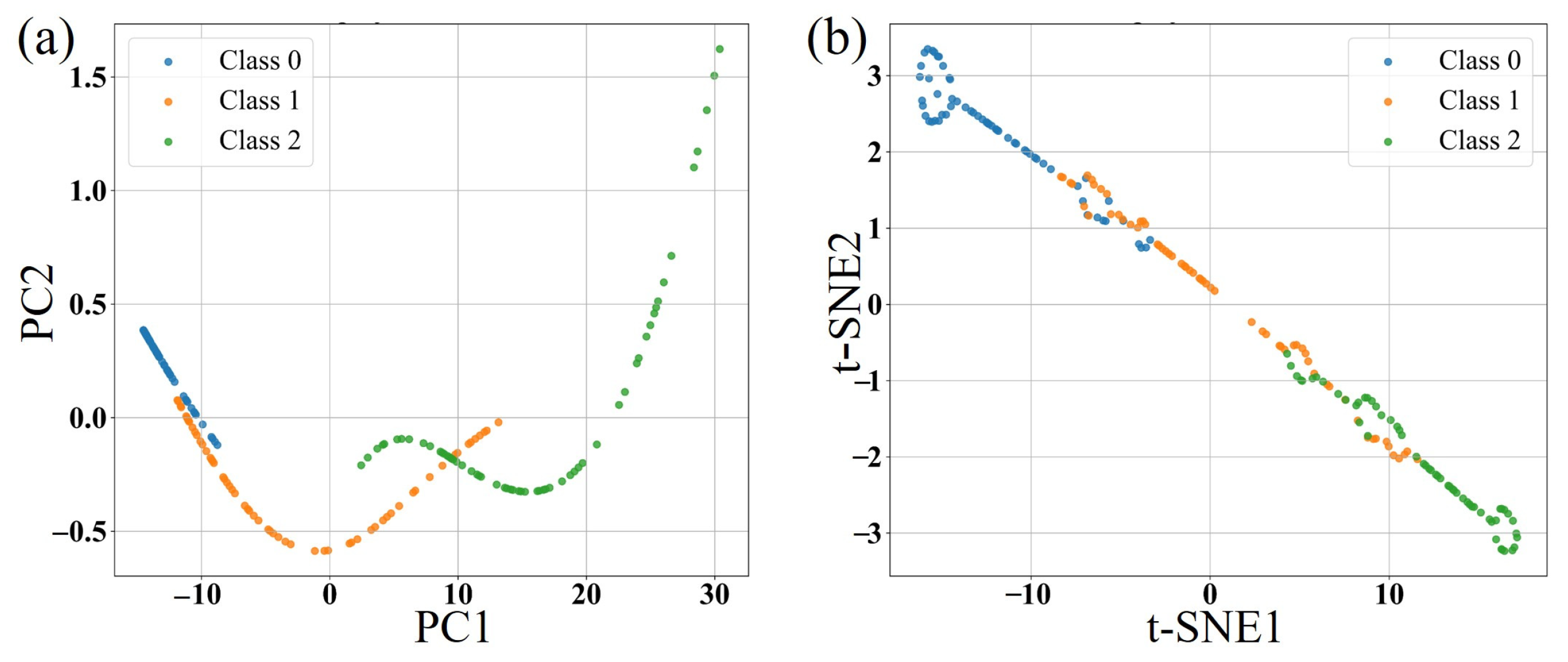
To investigate the origin of classification boundary ambiguity, Principal Component Analysis (PCA) [23,24] is employed for linear visualization of class separability, as shown in Figure 6a. The two-dimensional PCA projection indicates that the spherical tip samples are distributed between conical and flat classes, with partial overlap with both. Subsequently, a nonlinear dimensionality reduction technique, t-distributed stochastic neighbor embedding (t-SNE) [25,26], is employed to confirm boundary ambiguity between spherical tips and both conical and flat tips, as shown in Figure 6b. From combined PCA and t-SNE analyses, the spherical tip exhibits intermediate dynamic response characteristics between conical and flat geometries. This leads to its tendency to be misclassified into adjacent categories. In contrast, the conical and flat tips show a clear separation in the feature space, with no mutual misclassification.
Figure 6.
(a) 2D projection by PCA and (b) 2D projection by t-SNE in non-contact mode.
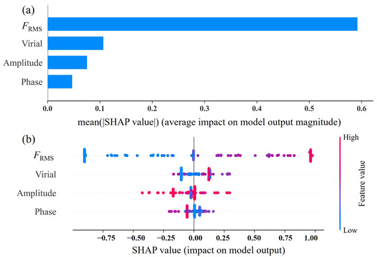
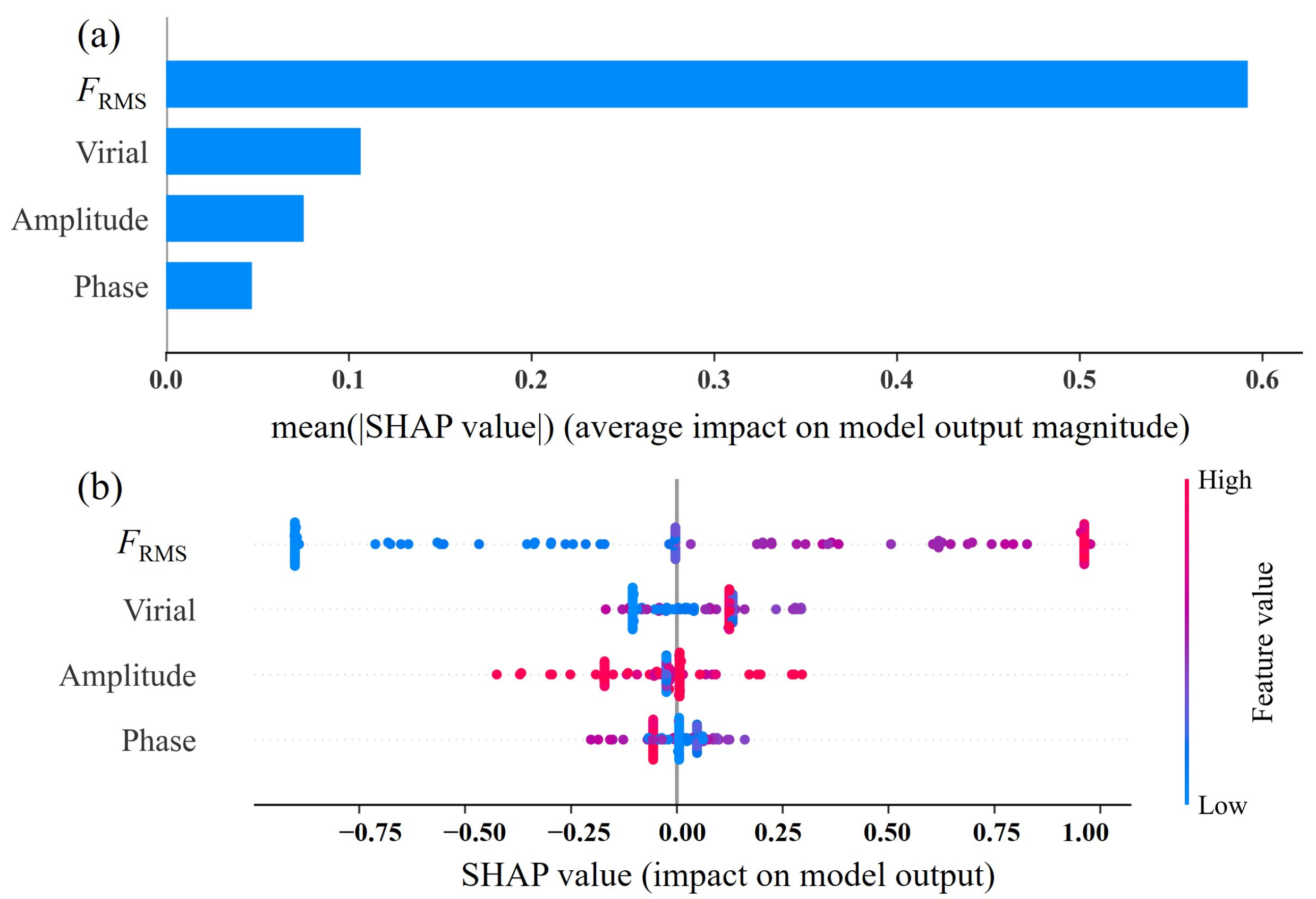
To gain deeper insight into the XGBoost decision-making mechanism and enhance interpretability, the SHAP method [27] is employed to quantify the contribution of each feature to model predictions, as shown in Figure 7. Based on the mean absolute SHAP value (Figure 7a), dimensionless FRMS exhibits an average contribution of approximately 0.6, significantly higher than other features, indicating it is the most critical feature reflecting the integrated strength and asymmetry of the tip–sample interaction. Virial feature ranks second, while phase shows the lowest global contribution.
Figure 7.
SHAP importance analysis results in non-contact mode: (a) bar plot, (b) bee swarm plot.
The SHAP bee swarm plot (Figure 7b) reveals feature value distribution patterns and their relative importance. The SHAP values of FRMS exhibit a pronounced bipolar distribution. Specifically, low FRMS values (blue points) are strongly associated with negative SHAP values, indicating that lower FRMS significantly increases the probability of assigning samples to a specific tip category. This observation is consistent with the physical behavior shown in Figure 3d, where the FRMS of the conical tip remains consistently the lowest, and also explains why spherical tips are more likely to be misclassified as conical. Conversely, high FRMS values (red points) correspond to positive SHAP values, indicating a strong tendency to predict flat tip prediction. This clearly separated bipolar pattern confirms that FRMS is the dominant discriminative feature and indirectly accounts for the unclear decision boundaries in the dimensionality reduction results. The virial feature shows a relatively concentrated SHAP distribution around zero. Higher virial values tend to produce positive SHAP contributions, serving as auxiliary discriminative information when FRMS values lie near the decision boundary. The SHAP distributions of amplitude and phase are more scattered, with weak correlations between feature magnitude and SHAP sign. These features therefore act as complementary inputs rather than primary determinants in the classification process.
To further elucidate the physical significance of the SHAP ranking, the feature importance is discussed from the perspective of the underlying tip–sample interaction mechanism. FRMS exhibits the highest contribution because it represents the root-mean-square value of the tip–sample interaction force over an oscillation cycle, simultaneously capturing both the magnitude and temporal characteristics of the interaction. Since different tip geometries produce distinct effective interaction areas and force gradients, they directly modify the nonlinear tip–sample interaction, making FRMS highly sensitive to variations in probe morphology. The virial ranks second in importance because it characterizes the conservative component of the tip–sample interaction and reflects the reversible energy exchange between the cantilever and the sample. Variations in probe geometry alter the interaction force gradient and conservative force field, resulting in distinguishable virial responses for different tip shapes. In contrast, the oscillation amplitude primarily reflects the overall dynamic response of the cantilever and is simultaneously influenced by excitation conditions, damping, and feedback control, making it less sensitive to differences in probe geometry. Similarly, the phase shift is a combined effect of tip–sample interaction, experimental parameters, and environmental factors, which reduces its discriminative capability compared with interaction-related descriptors. Thus, the SHAP importance ranking is physically consistent with the interaction dynamics of AFM, confirming that descriptors directly related to tip–sample interactions carry more geometry-specific information than global cantilever response variables.
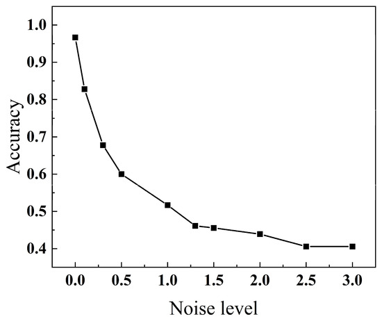
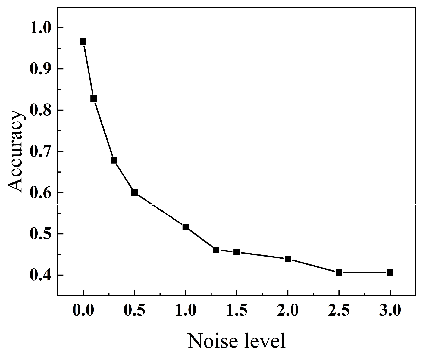
To comprehensively evaluate the robustness and generalization of the model under various perturbation conditions, systematic tests are performed from three aspects: noise perturbation, feature perturbation, and input distribution shift. For noise robustness analysis, zero-mean Gaussian noise with varying intensities (noise = 0.0~3.0) is directly added to the extracted feature vectors of the test set. The noise level is defined as the standard deviation of the Gaussian perturbation applied independently to each feature. This simplified feature-level perturbation assesses classifier robustness against input uncertainty, without explicitly modeling the propagation of measurement noise in raw AFM vibration signals. These datasets are then fed into the trained model for prediction to assess its sensitivity to stochastic measurement errors and the corresponding performance variation, as shown in Figure 8. When noise = 0, the model achieves an accuracy of 0.97. Under a low noise level (noise = 0.1), the performance remains relatively high at 0.83. As the noise intensity increases to 3.0, the accuracy decreases to 0.41. The model performance exhibits a smooth and monotonic degradation trend with increasing noise, without abrupt fluctuations or instability, indicating good anti-noise capability and strong robustness.
Figure 8.
Noise robustness variation trend in non-contact mode.
In the feature robustness analysis, a feature-wise perturbation strategy is adopted, where each of the input variables is independently perturbed while keeping the other features unchanged, evaluating the influence of individual physical descriptors on model stability. Results show that the model maintains relatively high classification accuracy under all single-feature perturbation conditions, with values of 0.85 for amplitude, 0.93 for phase, 0.93 for virial, and 0.92 for FRMS. The model is relatively insensitive to perturbations in any single feature, demonstrating good feature-level robustness. Overall, the model exhibits stable and gradual performance degradation under both Gaussian noise and feature perturbations, demonstrating good robustness within the current simulation framework.
4. Tip Shape Classification in Tapping Mode
4.1. Dynamic Model and Response Analysis in Tapping Mode
In tapping mode, the probe tip intermittently interacts with the sample surface during each oscillation cycle. The tip–sample interaction force consists of van der Waals attractive forces in the non-contact mode and elastic repulsive forces in the contact regime. The corresponding contact states for different tip geometries are illustrated in Figure 9, where a denotes the contact radius between the tip and the sample, and δ represents the indentation depth of the tip, defined as δ = a0 − d. The total tip–sample interaction force is expressed in a piecewise form:
where Fcontact represents the elastic contact force.
Figure 9.
Schematic diagram of tip–sample contact in tapping mode.
Based on the Sneddon model, the contact between an arbitrary axisymmetric tip and an elastic half-space is described [28]. By considering the tip and the sample as elastic bodies [29,30], the reduced elastic modulus E∗ is introduced:
where Es, vs, Et, and vt are the elastic moduli and Poisson’s ratios of the sample and the tip, respectively. The elastic contact force between a conical tip and the sample is:
The contact force between a spherical tip and the sample is expressed as:
The contact force between a flat tip and the sample is:
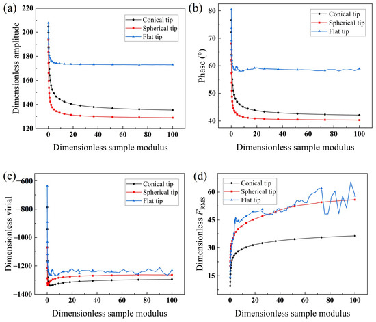
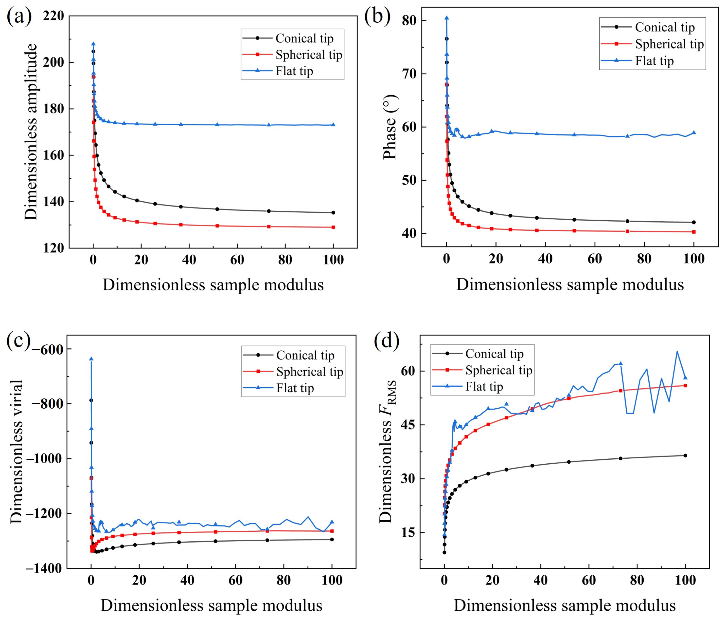
Substituting the above dimensional interaction forces into the second equation of Equation (6) yields the dimensionless forms. The dimensionless sample elastic modulus is defined as , with the reference modulus Eref =1 GPa. A sinusoidal displacement excitation with amplitude 5u0 is applied at the fixed end of the microcantilever, resulting in a dimensionless free oscillation amplitude of 212. The amplitude setpoints for the spherical and conical tips are set to 0.6, with the Hamaker constant set to be 10 × 10−20 J. Because the flat tip has a much larger effective interaction area, it experiences a substantially stronger attractive force than the conical and spherical tips under identical operating conditions. To maintain a stable and physically meaningful oscillation regime and to allow a fair comparison of the dynamic responses across tip geometries, the amplitude setpoint for the flat tip is increased to 0.8 to reduce the influence of the attractive interaction, while the Hamaker constant is set to 1 × 10⁻²⁰ J. The sample elastic modulus is within the range of 0.1~100 GPa, with 200 values sampled according to a logarithmic distribution.
As shown in Figure 10, when the sample elastic modulus is relatively low ( < 10), the dynamic response of the microcantilever undergoes significant variations. This is attributed to the soft materials’ proneness to elastic deformation during tip–sample interaction, leading to an increase in both the contact area and indentation depth. When the sample modulus is sufficiently high ( > 10), the response gradually becomes stable. With increasing sample elastic modulus, both the amplitude and phase of the conical and spherical tips decrease, while the FRMS gradually increases. The virial initially decreases rapidly, then slightly increases, and finally converges to a steady value. This can be explained by the transition of the dominant interaction mechanism. At low sample modulus, the attractive forces dominate, leading to a rapid decrease in virial. As the sample modulus increases, the repulsive forces gradually become dominant, resulting in an increase in virial. For the flat tip, due to its larger contact area and stronger adhesion effect, the amplitude, phase, virial, and FRMS consistently exhibit higher magnitudes. Moreover, even a small change in the sample modulus can induce pronounced variation in the contact force, resulting in noticeable fluctuation in the dynamic response.
Figure 10.
Dynamic responses of the microcantilever as a function of sample modulus for three tip shapes in tapping mode: (a) dimensionless amplitude, (b) phase, (c) dimensionless virial, (d) dimensionless FRMS.
4.2. XGBoost-Based Classification Model and Interpretability Analysis in Tapping Mode
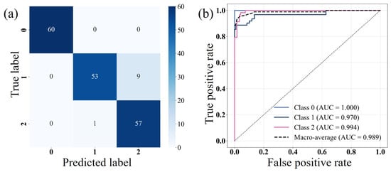
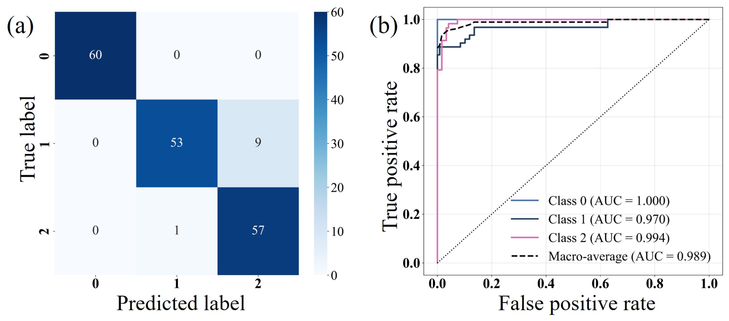
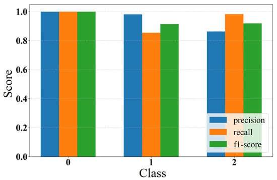
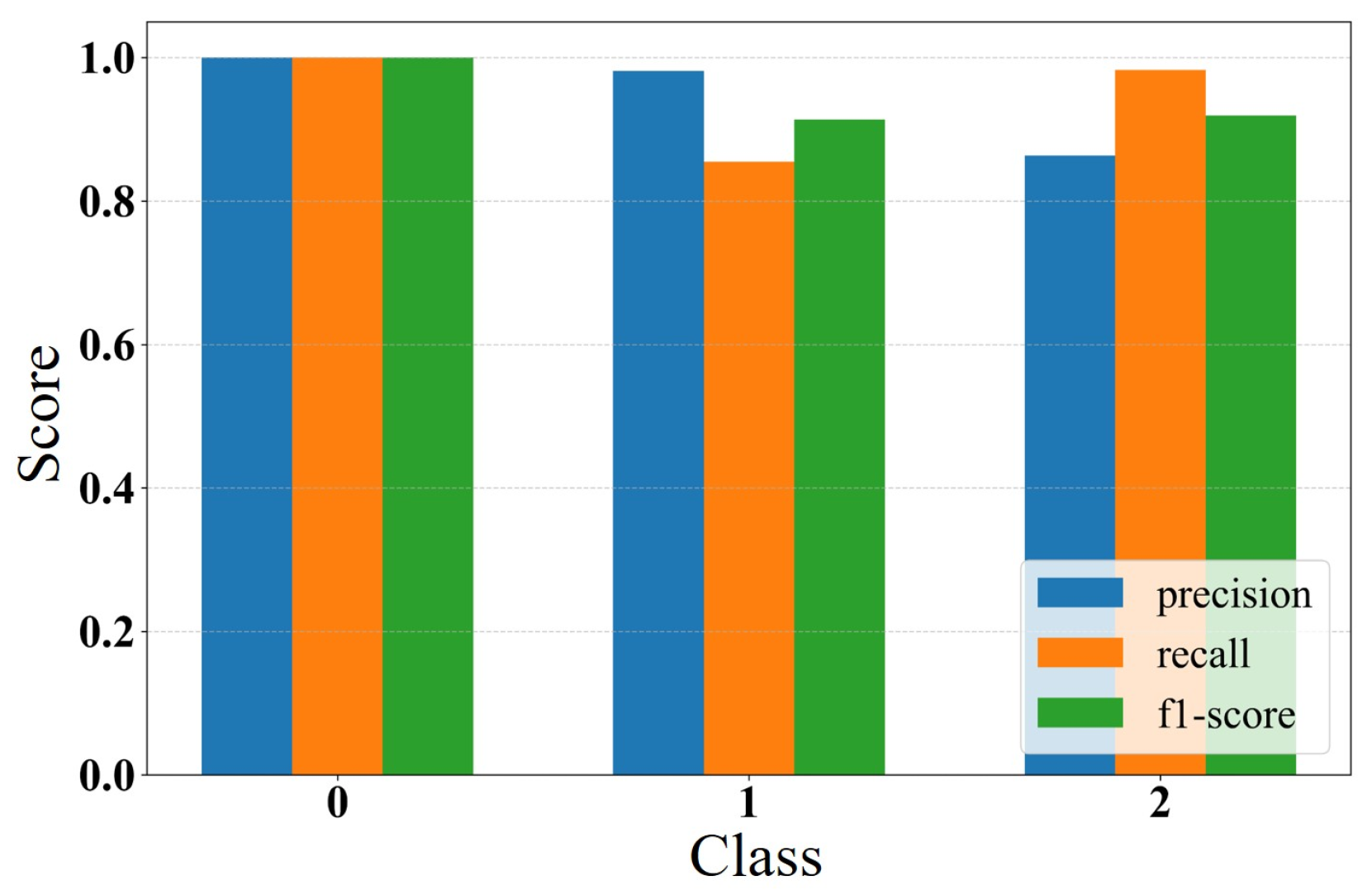
The dataset is combined and randomly shuffled, then divided into a training set and a test set with a ratio of 7:3. The input features consist of four dimensionless dynamic response quantities (amplitude, phase, virial, and FRMS), while the output corresponds to the tip class (conical: 0, spherical: 1, flat: 2). The same XGBoost parameter configuration as in the non-contact mode is adopted. The confusion matrix and ROC curves are shown in Figure 11. The conical tip prediction accuracy achieves 100%, consistent with its highest AUC value. The spherical tip yields an accuracy of 85.5%, while the flat tip reaches 98.3%. A certain deviation between classification accuracy and ROC-based AUC values is observed, mainly attributed to the suboptimal classification threshold selection. Nevertheless, the model still maintains high overall classification performance. The precision, recall, and F1-score distributions for the three tip geometries are shown in Figure 12. For the conical tip, all three metrics reach 1.0, indicating the highest feature separability and enabling perfect classification. For the spherical tip, precision is higher than recall, whereas for the flat tip, precision is lower than recall. However, all F1-scores exceed 0.9, demonstrating that the model maintains strong robustness and reliability even under tip–sample contact conditions.
Figure 11.
(a) Confusion matrix and (b) ROC curves for prediction results in tapping mode.
Figure 12.
Bar chart of classification performance metrics in tapping mode.
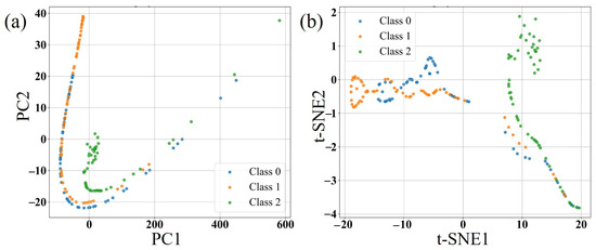
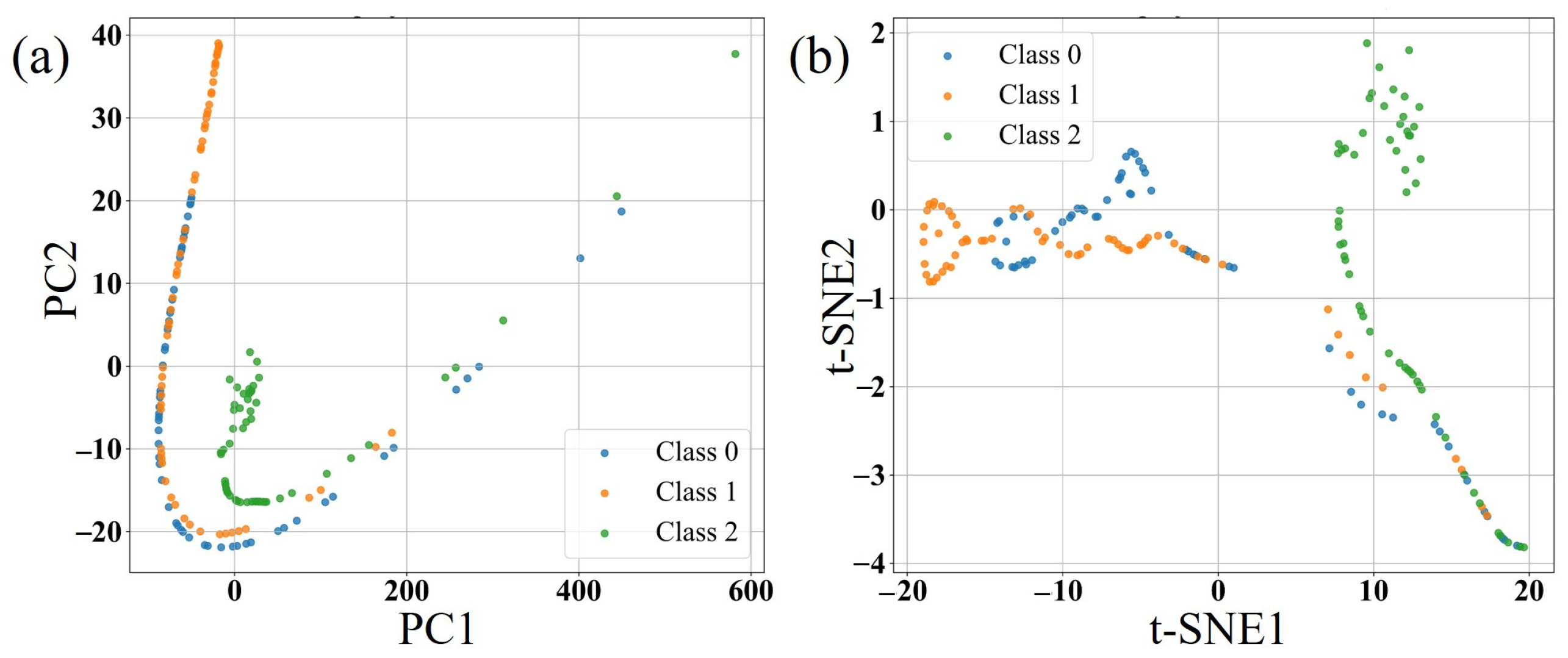
PCA is employed to visualize the boundaries of the three tip geometries, as shown in Figure 13a. The results indicate a clear clustering tendency in the two-dimensional feature space, with the flat tip samples being distinctly separated from the other two categories, suggesting that their dynamic response characteristics differ most significantly. However, since PCA only preserves directions of maximum variance, it is limited in capturing nonlinear structures and therefore has restricted discriminative capability for classes with high overlap. To address this limitation, t-SNE is further applied to capture nonlinear relationships, as shown in Figure 13b. It can be observed that t-SNE provides a clearer representation of nonlinear class boundaries. Nevertheless, partial overlap still exists between spherical and flat tip clusters, which explains the mutual misclassification between these two categories observed in the confusion matrix.
Figure 13.
(a) 2D projection by PCA and (b) 2D projection by t-SNE in tapping mode.
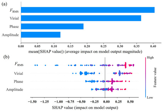
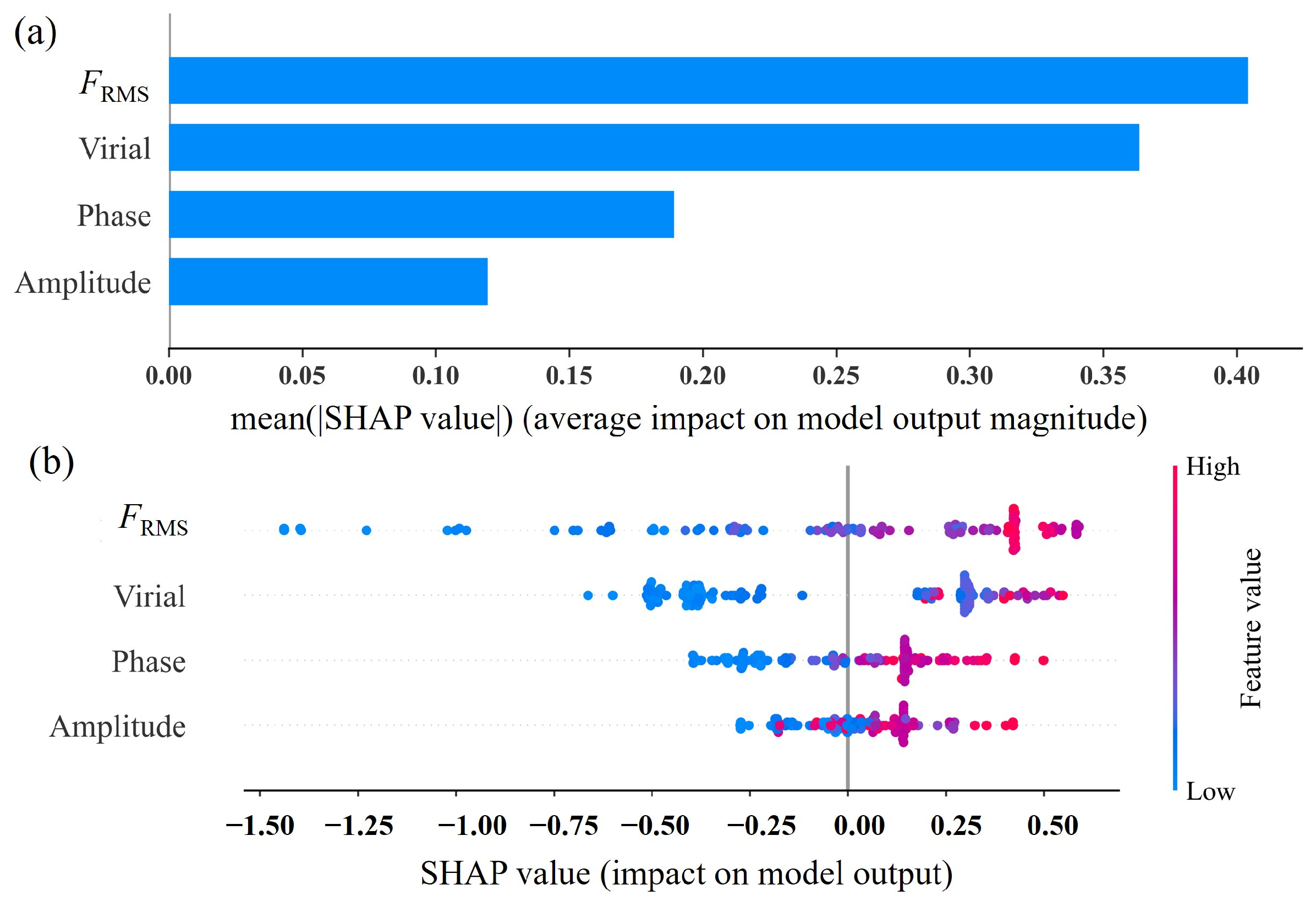
The SHAP method is employed to quantitatively evaluate the contribution of each feature to model predictions in tapping mode, as shown in Figure 14. The results indicate that the dimensionless FRMS and virial are the most influential features for classification, with significantly higher importance than amplitude and phase. High values of these two features tend to drive the model toward predicting a flat tip, whereas low values favor the conical tip class. This trend is consistent with the observed dynamic response characteristics, thereby providing mutual validation between the data-driven interpretability analysis and the underlying physical behavior.
Figure 14.
SHAP importance analysis results in tapping mode: (a) bar plot (b) bee swarm plot.
Compared with the non-contact mode, the amplitude and phase become more informative in tapping mode because the tip–sample interaction contains both attractive and repulsive components during each oscillation cycle. Under these conditions, the oscillation amplitude and phase are more directly influenced by contact-induced changes in energy exchange. Consequently, both features carry richer information about the interaction dynamics than in the non-contact mode, leading to higher contributions in the SHAP analysis. Nevertheless, their discriminative capability remains lower than that of the interaction-related descriptors because they are also affected by excitation conditions and feedback control. Compared with the non-contact mode, the increased importance of amplitude and phase further demonstrates that the transition from purely attractive interactions to combined attractive–repulsive interactions introduces additional dynamic information that benefits tip shape discrimination.
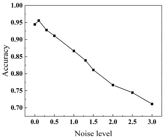
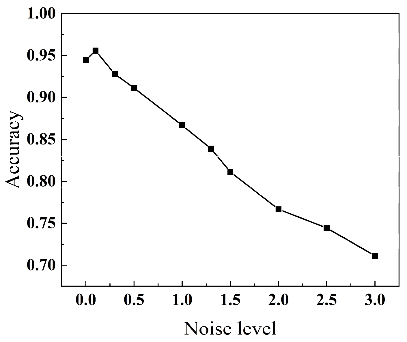
Based on the SHAP analysis, the FRMS and virial exhibit the highest importance in the model, dominating the overall classification decision process, while the contributions of amplitude and phase are relatively limited. To further investigate the role of each feature and the stability of the model, feature perturbation analysis and noise robustness tests are conducted. The results show that, in the feature-wise perturbation experiments, phase perturbation has the most significant impact on model performance, reducing the accuracy to 0.73. In contrast, perturbations in virial and amplitude lead to smaller performance degradations (0.92 and 0.90, respectively), while FRMS exhibits an intermediate effect (0.83). This indicates that although the phase has lower global importance in the SHAP ranking, it is highly sensitive to variations near decision boundaries and plays a critical role in distinguishing closely related classes. The noise robustness trend under tapping-mode operation is presented in Figure 15. Similar to the non-contact mode, the classification accuracy decreases gradually as the Gaussian noise level increases. At low noise levels (noise ≤ 0.3), the accuracy remains above 0.93, indicating that the model is relatively insensitive to small feature perturbations. As the noise level increases further, the classification accuracy gradually decreases (approximately 0.87 at noise = 1.0 and 0.71 at noise = 3.0), while exhibiting a smooth and monotonic degradation without abrupt fluctuations. These results further demonstrate that the model maintains stable classification performance under feature perturbations in the tapping mode.
Figure 15.
Noise robustness variation trend in tapping mode.
5. Conclusions
This study focuses on the problem of tip shape recognition in dynamic AFM and develops a systematic framework that integrates dynamic modeling, numerical simulation, and data-driven classification. By solving the dimensionless dynamic model using a finite difference method, the dynamic response characteristics of conical, spherical, and flat tips are systematically computed under both non-contact and tapping modes. Based on these results, an XGBoost-based classification model is constructed for tip shape identification. Furthermore, SHAP-based interpretability analysis and dimensionality reduction visualization techniques are employed to investigate the underlying classification mechanisms and boundary ambiguity. The main conclusions are summarized as follows:
- (1)
- The simulation results demonstrate that the dynamic response features of the microcantilever exhibit strong discriminative capability for the three tip geometries. Due to its larger contact area and stronger adhesive effects, the flat tip shows highly distinguishable behaviors in amplitude, phase, virial, and FRMS across the entire parameter range. In contrast, the conical tip, owing to its highly localized tip–sample interaction, is largely insensitive to variations in both the Hamaker constant and the sample elastic modulus, and thus exhibits higher stability and classification accuracy. These results indicate that tip shape information can be effectively characterized through dynamic response features of the microcantilever.
- (2)
- The XGBoost-based classification model achieves high accuracy on the simulated dataset, validating the feasibility of tip recognition driven by dynamic response features. In the non-contact mode, the overall test accuracy reaches 96.7%, with a 100% recognition rate for conical tips. In the tapping mode, the model maintains a high level of performance, with classification accuracies of 100%, 85.5%, and 98.3% for conical, spherical, and flat tips, respectively. Moreover, the model exhibits stable and well-controlled performance degradation under various typical uncertainty conditions, demonstrating strong robustness.
- (3)
- SHAP analysis identifies FRMS and virial as the dominant discriminative features in both operating modes, which is physically consistent with the underlying tip–sample interaction mechanisms. Compared with amplitude and phase, these interaction-related descriptors provide more direct information about probe geometry, thereby contributing more significantly to the classification performance.
- (4)
- The classification ambiguity between spherical and flat tips can be attributed to the similarity in mechanical responses of the two contact mechanisms within a specific transition range of sample elastic modulus. This finding provides guidance for further optimization of the feature set. Nevertheless, the present study is confined to an idealized simulation framework. Although the simulated datasets are generated from a physics-based dynamic AFM model, they do not fully capture practical factors encountered in real AFM measurements, such as instrumental noise, environmental disturbances, tip contamination, calibration errors, and manufacturing variability. Therefore, the applicability of the framework under experimental conditions requires further validation. Moreover, the training and testing datasets are randomly partitioned from the same simulation database. While this strategy is appropriate for evaluating the classification capability within the current parameter space, it essentially reflects interpolation within a single data distribution and may yield optimistic performance estimates when applied to different operating conditions. Future work will incorporate experimentally acquired AFM data, explore more realistic tip morphologies, introduce realistic measurement noise into the simulated cantilever time-domain signals prior to feature extraction, and systematically evaluate the framework to further assess its robustness and generalization capability.
Author Contributions
Conceptualization, Z.Z. and X.Z.; methodology, Z.Z. and X.Z.; validation, Z.Z. and B.H.; formal analysis, Z.Z. and B.H.; investigation, Z.Z. and B.H.; visualization, Z.Z. and B.H.; writing—original draft preparation, Z.Z.; writing—review and editing, X.Z.; supervision, X.Z. All authors have read and agreed to the published version of the manuscript.
Funding
This research was funded by the open foundation of Hubei Key Laboratory of Theory and Application of Advanced Materials Mechanics (Wuhan University of Technology) under Grant No. TAM202205.
Data Availability Statement
The supporting data for this study can be obtained from the corresponding author upon reasonable request.
Conflicts of Interest
The authors declare no conflicts of interest.
References
- Garcia, R. Amplitude Modulation Atomic Force Microscopy; Wiley-VCH: Weinheim, Germany, 2010. [Google Scholar]
- Kopycinska-Müller, M.; Geiss, R.H.; Hurley, D.C. Contact mechanics and tip shape in AFM-based nanomechanical measurements. Ultramicroscopy 2006, 106, 466–474. [Google Scholar] [CrossRef] [Scilit] [PubMed]
- Kopycinska-Müller, M.; Geiss, R.H.; Rice, P.; Hurley, D.C. Influence of tip wear on atomic force acoustic microscopy experiments. Scanning-Probe Other Nov. Microsc. Local Phenom. Nanostruct. Mater. 2004, 838, 25–30. [Google Scholar] [CrossRef] [Scilit]
- Killgore, J.P.; Geiss, R.H.; Hurley, D.C. Continuous Measurement of Atomic Force Microscope Tip Wear by Contact Resonance Force Microscopy. Small 2011, 7, 1018–1022. [Google Scholar] [CrossRef] [Scilit] [PubMed]
- Liu, J.; Notbohm, J.; Carpick, R.W.; Turner, K.T. Method for characterizing nanoscale wear of atomic force microscope tips. ACS Nano 2010, 4, 3763–3772. [Google Scholar] [CrossRef] [Scilit] [PubMed]
- Li, Y.; Zhang, L.; He, Y. Wear of monocrystalline silicon AFM tips under extremely high frequency tapping. Wear 2025, 571, 205809. [Google Scholar] [CrossRef] [Scilit]
- Huang, S.; Tian, Y.; Wang, T. Experimental investigation of tip wear of AFM monocrystalline silicon probes. Sensors 2023, 23, 4084. [Google Scholar] [CrossRef] [Scilit] [PubMed]
- VanLandingham, M.R.; Juliano, T.; Hagon, M. Measuring tip shape for instrumented indentation using atomic force microscopy. Meas. Sci. Technol. 2005, 16, 2173–2185. [Google Scholar] [CrossRef] [Scilit]
- Nguyen, Q.D.; Chung, K.-H. Effect of tip shape on nanomechanical properties measurements using AFM. Ultramicroscopy 2019, 202, 1–9. [Google Scholar] [CrossRef] [Scilit] [PubMed]
- Labuda, A.; Kocuń, M.; Meinhold, W.; Walters, D.; Proksch, R. Generalized Hertz model for bimodal nanomechanical mapping. Beilstein J. Nanotechnol. 2016, 7, 970–982. [Google Scholar] [CrossRef] [Scilit] [PubMed]
- Bellotti, R.; Picotto, G.B.; Ribotta, L. AFM measurements and tip characterization of nanoparticles with different shapes. Nanomanuf. Metrol. 2022, 5, 127–138. [Google Scholar] [CrossRef] [Scilit]
- Yu, M.; Zhu, L.; Yang, Z.; Ning, J.; Xue, P.; Wang, S.; Wang, L.; Tan, X. Machine learning-assisted process-structure-property correlation in laser metal additive manufacturing: A critical review. Int. J. Extrem. Manuf. 2026, 8, 042005. [Google Scholar] [CrossRef] [Scilit]
- Elsherbiny, L.; Santos, S.; Gadelrab, K.; Olukan, T.; Font, J.; Barcons, V.; Chiesa, M. Machine learning assisted multifrequency AFM: Force model prediction. Appl. Phys. Lett. 2023, 123, 231603. [Google Scholar] [CrossRef] [Scilit]
- Matsunaga, Y.; Fuchigami, S.; Ogane, T.; Takada, S. End-to-end differentiable blind tip reconstruction for noisy atomic force microscopy images. Sci. Rep. 2023, 13, 129. [Google Scholar] [CrossRef] [Scilit] [PubMed]
- Nalluri, M.; Pentela, M.; Eluri, N.R. A scalable tree boosting system: XG Boost. Int. J. Res. Sci. Eng. Technol. 2020, 7, 36–51. [Google Scholar]
- Yu, M.; Zhu, L.; Yang, Z.; Ning, J. In-situ monitoring and ensemble learning for micro-pore distribution prediction in laser-directed energy deposition. Eng. Appl. Artif. Intell. 2026, 174, 114496. [Google Scholar] [CrossRef] [Scilit]
- Alizamir, M.; Wang, M.; Ikram, R.M.A.; Gholampour, A.; Ahmed, K.O.; Heddam, S.; Kim, S. An interpretable XGBoost-SHAP machine learning model for reliable prediction of mechanical properties in waste foundry sand-based eco-friendly concrete. Results Eng. 2025, 25, 104307. [Google Scholar] [CrossRef] [Scilit]
- Alizamir, M.; Wang, M.; Ikram, R.M.A.; Ahmed, K.O.; Heddam, S.; Kim, S. An efficient computational investigation on accurate daily soil temperature prediction using boosting ensemble methods explanation based on SHAP importance analysis. Results Eng. 2024, 24, 103220. [Google Scholar] [CrossRef] [Scilit]
- Gady, B.L. Measurement of Interaction Forces Between Micrometer-Sized Particles and Flat Surfaces Using an Atomic Force Microscope. PhD Thesis, Purdue University, West Lafayette, IN, USA, 1996. [Google Scholar]
- Feng, B.; Li, Y.; Li, R.; Li, H. Error analysis in calculation and interpretation of AFM tip-surface interaction forces. Adv. Colloid Interface Sci. 2022, 306, 102710. [Google Scholar] [CrossRef] [Scilit] [PubMed]
- Desemo, M.; Holm, C. How to mesh up Ewald sums (ii): An accurate error estimate for the P3M algorithm. J. Chem. Phys. 1998, 109, 7694–7701. [Google Scholar]
- Menga, N.; Bottiglione, F.; Carbone, G. The nonlinear dynamic behavior of a Rubber-Layer Roller Bearing (RLRB) for vibration isolation. J. Sound Vib. 2019, 463, 114952. [Google Scholar] [CrossRef] [Scilit]
- Candès, E.J.; Li, X.; Ma, Y.; Wright, J. Robust principal component analysis? J. ACM 2011, 58, 11:1–11:37. [Google Scholar] [CrossRef] [Scilit]
- Murariu, G.; Dinca, L.; Munteanu, D. Trends and applications of principal component analysis in forestry research: A literature and bibliometric review. Forests 2025, 16, 1155. [Google Scholar] [CrossRef] [Scilit]
- Van Der Maaten, L. Accelerating t-SNE using tree-based algorithms. J. Mach. Learn. Res. 2014, 15, 3221–3245. [Google Scholar] [CrossRef] [Scilit]
- Iwasaki, K.; Hino, H. Dynamics of the accelerated t-SNE. Trans. Mach. Learn. Res. 2025. [Google Scholar] [CrossRef] [Scilit]
- Lundberg, S.; Lee, S.-I. A unified approach to interpreting model predictions. Adv. Neural Inf. Process. Syst. 2017, 30, 4768–4777. [Google Scholar]
- Sneddon, I.N. The relation between load and penetration in the axisymmetric Boussinesq problem for a punch of arbitrary profile. Int. J. Eng. Sci. 1965, 3, 47–57. [Google Scholar] [CrossRef] [Scilit]
- Pharr, G.; Oliver, W.; Brotzen, F.R. On the generality of the relationship among contact stiffness, contact area, and elastic modulus during indentation. J. Mater. Res. 1992, 7, 613–617. [Google Scholar] [CrossRef] [Scilit]
- Gisbert, V.G.; Garcia, R. Insights and guidelines to interpret forces and deformations at the nanoscale by using a tapping mode AFM simulator: dForce 2.0. Soft Matter 2023, 19, 5857–5868. [Google Scholar] [CrossRef] [Scilit] [PubMed]



Disclaimer/Publisher’s Note: The statements, opinions and data contained in all publications are solely those of the individual author(s) and contributor(s) and not of MDPI and/or the editor(s). MDPI and/or the editor(s) disclaim responsibility for any injury to people or property resulting from any ideas, methods, instructions or products referred to in the content. |
© 2026 by the authors. Licensee MDPI, Basel, Switzerland. This article is an open access article distributed under the terms and conditions of the Creative Commons Attribution (CC BY) license.