SpatioConvGRU-Net for Short-Term Traffic Crash Frequency Prediction in Bogotá: A Macroscopic Spatiotemporal Deep Learning Approach with Urban Factors

Abstract

Traffic crashes represent a major challenge for road safety, public health, and mobility management in complex urban environments, particularly in metropolitan areas characterized by intense traffic flows, high population density, and strong commuter dynamics. The development of short-term traffic crash prediction models represents a fundamental line of analysis in road safety research within the scientific community. Among these efforts, macro-level modeling plays a key role by enabling the analysis of the spatiotemporal relationships between diverse factors at an aggregated zonal scale. However, in cities like Bogotá, predicting short-term traffic crashes remains challenging due to the complexity of these spatiotemporal dynamics, underscoring the need for models that more effectively integrate spatial and temporal data. This paper presents a strategy based on deep learning techniques to predict short-term spatiotemporal traffic crashes in Bogotá using 2019 data on socioeconomic, land use, mobility, weather, lighting, and crash records across TMAU and TAZ zones. The results showed that the strategy performed with a model called SpatioConvGru-Net with top performance at the TMAU level, achieving $R^2$ = 0.983, MSE = 0.017, and MAPE = 5.5%. Its hybrid design captured spatiotemporal patterns better than CNN, LSTM, and others. Performance improved at the TAZ level using transfer learning.

1. Introduction

Road safety in urban environments is constantly monitored for its cross-cutting impact on health, the economy, and mobility. Analyzing the spatial variations in traffic crashes using zonal covariates has become a key approach in road safety research for the scientific community. Different studies have identified positive relationships between environmental variables such as precipitation, humidity, temperature, and lighting on the increase in traffic crashes [1,2,3]. Others have recognized the importance of including inherent factors of the place where these events occurred, such as land use, socioeconomic stratification, households, and population density [4,5,6,7,8]. Others have found that mobility variables such as traffic, travel by different means of transport, and transport speed directly affect traffic crashes [9,10,11,12,13]. The level of spatial aggregation is another determining factor for studying traffic crash rates. There are different spatial units that have been used for this purpose such as Transportation Analysis Zones (TAZ) [4,5,6,9,10,11,14,15,16,17], wards [12], census tracts [7,8,18], and basic geostatistical areas (AGEB) [19]. Analyzing traffic crashes at the area level allows, on the one hand, the establishment of links between covariates and the frequency of these events. On the other hand, such an analysis allows for predicting the risk of traffic crashes. This ultimately makes it possible to assess the degree of safety for a geographical unit [17]. In relation to the above, several authors point out the importance of predicting traffic crashes in the short term ([20,21,22]). This is because the phenomenon of traffic crashes is affected by environmental and mobility factors that exhibit high spatiotemporal variation [23]. For example, Kashifi et al. identified that spatiotemporal variables such as traffic, average road speed, vehicle kilometers traveled, and weighted average occupancy have a great impact on traffic crashes [24]. For their part, ref. [2] found that variables such as temperature, precipitation, snowfall, pressure, and wind speed captured at the hourly level dynamically impact traffic crashes at the zonal level over time. This is relevant given that to proactively address the dynamic spatiotemporal behavior of traffic crashes, detailed knowledge of the when, where, and why of this phenomenon is required. The applicability of conventional approaches based on classical statistical models has performed unsatisfactorily in practical situations [25]. Recent studies support that deep learning methods such as Convolutional Neural Networks (CNN), Recurrent (RNN) and Long Short Learning (LSTM) have superior performance for short-term traffic crash prediction [2,24]. This is achieved due to their architectures, which can learn complex and nonlinear structures present in the data, such as hidden spatiotemporal heterogeneities ([2,24]).

The main objective of this study is to propose a strategy based on a deep learning model for citywide short-term spatiotemporal crash prediction at an hourly resolution, using socioeconomic, environmental, land use, and mobility variables. This granularity is crucial in a city like Bogotá, where traffic conditions vary significantly between peak and off-peak hours, especially in areas with a high concentration of the working population. The inclusion of land use data helps characterize these temporal-spatial dynamics, enabling more targeted and timely preventive actions, such as the real-time deployment of emergency services and dynamic traffic flow adjustments

The contributions of this paper can be summarized as follows: (a) We propose a strategy based on a spatiotemporal hybrid deep learning architecture that allows the simultaneous exploration of spatial and temporal dependencies present in high-dimensional independent variables, using the extraction of features that are distributed and organized in hierarchical levels. (b) The proposed architecture presents an effective performance in the detailed prediction of traffic crashes, providing precision in the identification of the location and time of occurrence. (c) The proposed index as a variable of interest allows approaching a practical and real analysis of traffic crashes, since it seeks to represent this phenomenon as punctual patterns on the network and as real counts of area data. The rest of the document is structured as follows: In the next section, the study area and data are presented. This is followed by a concise description of the method employed in this research for the proposed strategy and the data collected to test the model. The results and evaluation of the modeling are then presented. Finally, the predictive performance of the models is discussed, and the conclusions and recommendations of this study are proposed.

2. Materials and Methods

The methods proposed in this study focus on the use of deep learning models to predict short-term traffic crashes in the urban area of Bogota based on socioeconomic, environmental, land use, and mobility variables. A hybrid spatiotemporal convolutional neural network model with recurrent unit gating and short- and long-term memory (SpatioConvGru-Net) was built with substantial modifications of the SCTL-Net model previously used by [2]. The architecture of this model obeys a heterogeneous type of neural network ensemble model. This integrates three different sub-models: convolutional neural network (CNN), recurrent neural network (GRU), and convolutional neural network for short- and long-term memory (ConvLSTM). The training, evaluation, and validation of the ensemble model were performed on the TMAU major scale data. Subsequently, the model underwent fine-tuning to be validated on a more detailed geographic scale, TAZ, to evaluate its predictive performance on smaller spatial units. In this section, a brief discussion of the structure of the previously mentioned models and the implemented tuning is given.

2.1. SpatioConvGru-Net Ensemble Model Structure

The proposed SpatioConvGru-Net model is an adaptation of the base model from [2], which merges high-level features extracted from three spatial, temporal, and spatiotemporal components. Its results exposed a remarkably predictive performance in spatiotemporal sequence prediction problems. The substantial difference is presented in the proposal to use the GRU model with a simplified structure with respect to the LSTM for learning temporal patterns. Additionally, the process of implementing regularization, dropout, and batch normalization strategies aims to improve the model’s generalization. In this sense, the neural network ensemble model SpatioConvGru-Net stands as an effective compendium of three models specialized in capturing complex patterns involving both spatial and temporal variations present in the phenomenon of traffic crashes. Its effectiveness in this application is due to its ability to combine by averaging the outputs of the individual models specialized in learning spatial (CNN), temporal (GRU) and spatiotemporal (ConvLSTM) patterns present in the different types of variables. These can be seen in Table 1 and the description of the types is presented below:

Table 1. Description of variables.

Category	Variable	Name	Description
Type I	Land use factors
	LU	Land uses	Allocation of land use according to the activities that can be developed there: residential, commercial, and industrial.
	ST	Socioeconomic stratification	Predominant classification of residential properties: 1 (low-low), 2 (medium-low), 3 (medium-medium), 4 (medium), 5 (medium-high) and 6 (high).
Type I	Socioeconomical Factors
	PD	Population density	Demographic distribution of the number of inhabitants per km2.
	RMMV	Rate of motorization of motor vehicles	Number of motorized vehicles with license plates per 1.000 inhabitants (reflects the number of vehicles owned by the population in the territory).
	NH	Number of households	Number of households (residential units) per spatial unit.
	Mobility factors
	RPTP	Rate of pedestrian trips per person	Hourly average of pedestrian trips equal to or greater than 15 min per person
	RTPPT	Rate of trips per person in public transport	Hourly average of public transportation trips per person
	RTPT	Rate of trips per person by taxi	Hourly average of taxi trips per person
	RTPC	Rate of trips per person by car	Hourly average of automobile trips (light vehicles: sedan, compact, sport utility, camper, truck, pick up and van) per person.
	RTPM	Rate of trips per person on motorcycle	Hourly average of motorcycle trips per person
	RTPB	Rate of trips per person by bicycle	Hourly average of bicycle trips per person
	TTDOD	Trips in a typical day origin-destination	Total of origin (produced) and destination (attracted) trips per hour across all available modes of transportation.
	TRPTM	Travel rate per person in BRT system	Hourly average of BRT system trips per person.
	AMSA	Average maximum speed allowed	Average maximum allowable speed in km/h of the total number of road segments contained in each spatial unit.
Type II	Environmental factors
	PCP	Precipitation	Total hourly precipitation in millimeters (mm). One millimeter means that one liter of water fell on each square meter of land.
	ILLUM	Illumination	Presence of ambient light in an environment. It can vary according to the time of day: optimal during daylight hours and limited during the night.
Type III	Response variable
	TCIRP	Traffic Crashes Index on the road perimeter	Rate of traffic crashes per hour in total kilometers of roadway per one spatial unit.

• Type I Variables: These vary spatially but are static in the time of the study period, since they were originally collected during an annual period. For this type of variable, the spatial dependence present between spatial units is considered. Examples include population density, land use, socioeconomic stratification, among others.
• Type II Variables: These vary temporally but are spatially static over the time of the study. This study considers environmental variables such as precipitation and illumination that are constant in space throughout the study area and for which temporal dependence is considered.
• Type III Variables: These vary spatially and temporally over the study period. This category includes only the variable of interest, the Traffic Crashes Index on the road perimeter, as it exhibits both local and spatial dependence simultaneously.

To develop the capabilities of the SpatioConvGru-Net model, it was necessary to organize and process spatial, temporal, and spatiotemporal data obtained from multiple external sources. The following section describes and characterizes these datasets as a foundation for the subsequent definition and specification of the proposed models.

The integration of CNN, GRU, and ConvLSTM architectures in the proposed model is grounded in the need to capture different types of dependencies inherent in traffic crash phenomena. CNN modules extract spatial features from static variables such as socioeconomic and land use indicators; GRU modules model sequential patterns from temporal variables like weather and illumination and ConvLSTM layers are well-suited to learn spatiotemporal dynamics from variables that vary across both dimensions, such as crash intensity. While alternative models—such as tree-based algorithms like CatBoost or XGBoost—are effective in certain regression tasks, they do not inherently model temporal sequences or spatial structures. Therefore, a neural network-based approach was selected due to its superior ability to learn non-linear, high-dimensional patterns with temporal and spatial coherence, which are essential in modeling urban traffic crashes.

2.2. Data

To develop the SpatioConvGru-Net accident predicting model, we collected data from 2019 in Bogotá, Colombia. The study area covered the city’s urban zones, divided into 110 Territorial Mobility Analysis Units (TMAU), along with a finer scale known as the Transportation Analysis Zone (TAZ) [5,6,9,10,14,16,17].

The Territorial Mobility Analysis Units (TMAU) and Transportation Analysis Zones (TAZ) are official spatial divisions defined by Bogotá’s Secretariat of Mobility. These zonings are widely used in transportation planning and analysis due to their homogeneity in terms of land use, population density, and mobility behavior. They represent the most operationally relevant spatial units for which crash data and other key variables are systematically collected and available. Furthermore, the use of TAZs has been widely adopted in previous research as an appropriate spatial scale for traffic accident prediction and risk modeling [4,5,6,9,10,11,12,14,15,16,17]. Their selection ensures both methodological consistency and practical applicability of the predictive model for urban mobility management

Three types of data were used: spatial (socioeconomic, land use, and mobility indicators), temporal (hourly precipitation and illumination), and spatiotemporal (traffic crashes). The information was obtained from official sources, including SIMUR (Integrated Information System on Regional Urban Mobility [26]), IDEAM (Institute of Hydrology, Meteorology and Environmental Studies [27]), and Datos Abiertos Bogotá (Open Data Bogota [28]). The SIMUR platform provides open access to data on urban and regional mobility in Bogotá and surrounding areas. It supports planning, decision-making, and public transparency through geospatial and statistical mobility data. IDEAM is Colombia’s national agency responsible for monitoring and analyzing hydrological, meteorological, and environmental conditions. It offers public access to the climate, weather, and environmental datasets critical for research and policy development. OpenDataBogotá is the official open data portal of the Bogotá City Government. It provides a wide range of datasets across sectors to promote transparency, innovation, and civic engagement.

The integration of the alphanumeric socioeconomic, land use, mobility, and travel matrix information with the TMAU and TAZ was performed through a joint operation, using the identifiers shared between the alphanumeric tables and the polygon attributes. The original information was expanded to a time series whose minimum unit was the hour and generated a dataset of 963,400 records (110 TMAU spatial units × 24 h × 365 days). The hourly precipitation variable was incorporated with the hourly measurements of the meteorological stations closest to the centroid of each of the spatial units using the nearest Euclidean distance as an assignment criterion. The illumination variable was categorized into two mutually exclusive classes covering the full 24-h cycle: optimal (from 06:00 inclusive to 17:00 exclusive) and limited (from 17:00 inclusive to 06:00 exclusive of the next day). These intervals were extracted from the hourly time series data.

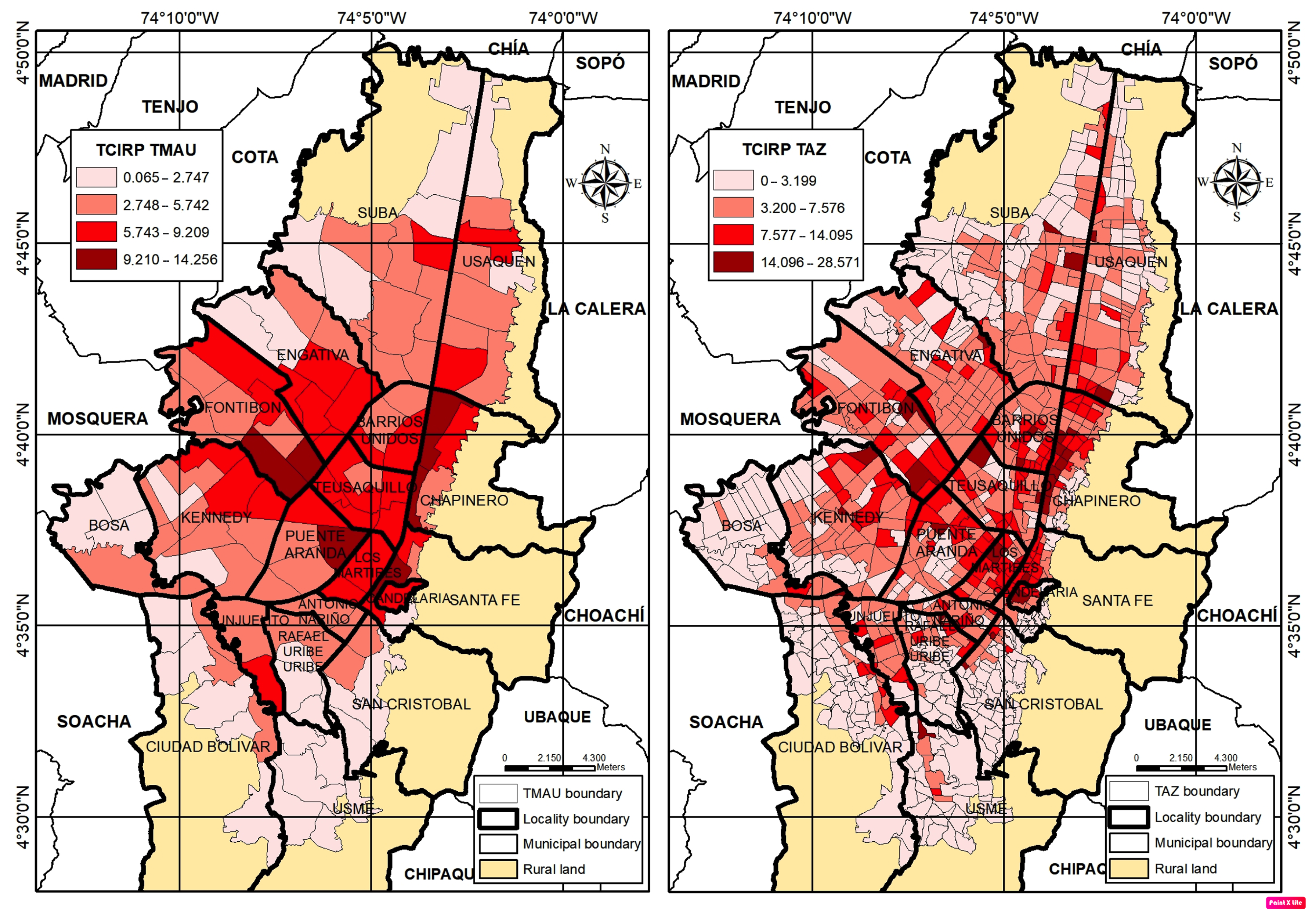
The variable of interest in this research corresponds to the Traffic Crashes Index on the Road Perimeter (TCIRP) that aims to relate the frequency of traffic crashes on the roads with the macroscopic factors of the spatial units [13]. The construction of this variable was carried out through multiple geoprocesses using Geopandas and GDAL Python libraries. The geolocation information, date, and time of traffic crash records and the alphanumeric spatial information of the Malla Vial Integral de Bogotá. (MVI) available in the online services of Datos Abiertos Bogotá (Bogotá Open Data) were used. In the first instance, the total perimeter in kilometers of the road sections per spatial unit was calculated, then the count of traffic crashes per hour/spatial unit was generated to finally calculate the TCIRP as shown in Equation (1):

$$TCIRP={\displaystyle \frac{\mathrm{number}\mathrm{of}\mathrm{traffic}\mathrm{crashes}\mathrm{per}\mathrm{hour}/\mathrm{space}\mathrm{unit}}{\mathrm{total}\mathrm{length}\mathrm{in}\mathrm{kilometers}\mathrm{of}\mathrm{road}\sec \mathrm{tions}\mathrm{per}\mathrm{spatial}\mathrm{unit}}}$$

(1)

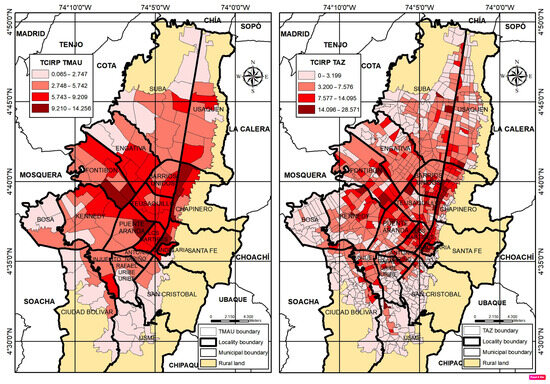
The spatial distribution of the TCIRP for the TMAU and TAZ can be seen in Figure 1.

Figure 1. Spatial distribution of TCIRP at the TMAU level (on the left) and the TAZ level (on the right) in the study area, segmented using natural breaks classification (Authors).

In total, a dataset of sixteen (16) independent variables was consolidated, of which two (2) were nominal (LU and ST), two (2) numerically discrete (PD and NH), and the remaining numerically continuous. The dependent variable is a continuous numerical variable. The variables considered in the present study are described in Table 1.

Spatiotemporal Cross-Validation Approach

To ensure a robust evaluation of the model’s predictive performance while accounting for the spatiotemporal structure of the data, a two-step validation strategy was adopted. First, a temporal hold-out validation was implemented. The training and test datasets were partitioned chronologically to avoid data leakage across time. Specifically, the model was trained using data from earlier time periods and tested on subsequent, non-overlapping temporal blocks. This approach prevents the model from being exposed to future information during training, thereby mitigating the temporal autocorrelation bias in the performance assessment. Second, we assessed the spatial independence of the residuals by computing Moran’s I statistic over the zonal residuals aggregated at the prediction level. This analysis was conducted using queen contiguity criteria for spatial weights and implemented with the PySAL library v4.13. The resulting Moran’s I values indicated low and non-significant spatial autocorrelation in the residuals across zones, suggesting that the model does not systematically under- or over-predict in geographically clustered regions. The results of the spatial autocorrelation analysis on the residuals are summarized in Table 2.

Table 2. Moran’s I spatial autocorrelation analysis.

Spatial Unit	Moran’s I	Z-Score	p-Value
TMAU	0.018	0.742	0.457
TAZ	−0.012	−0.594	0.552

2.3. Proposed Model

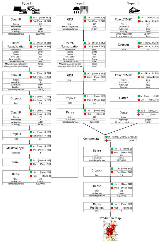
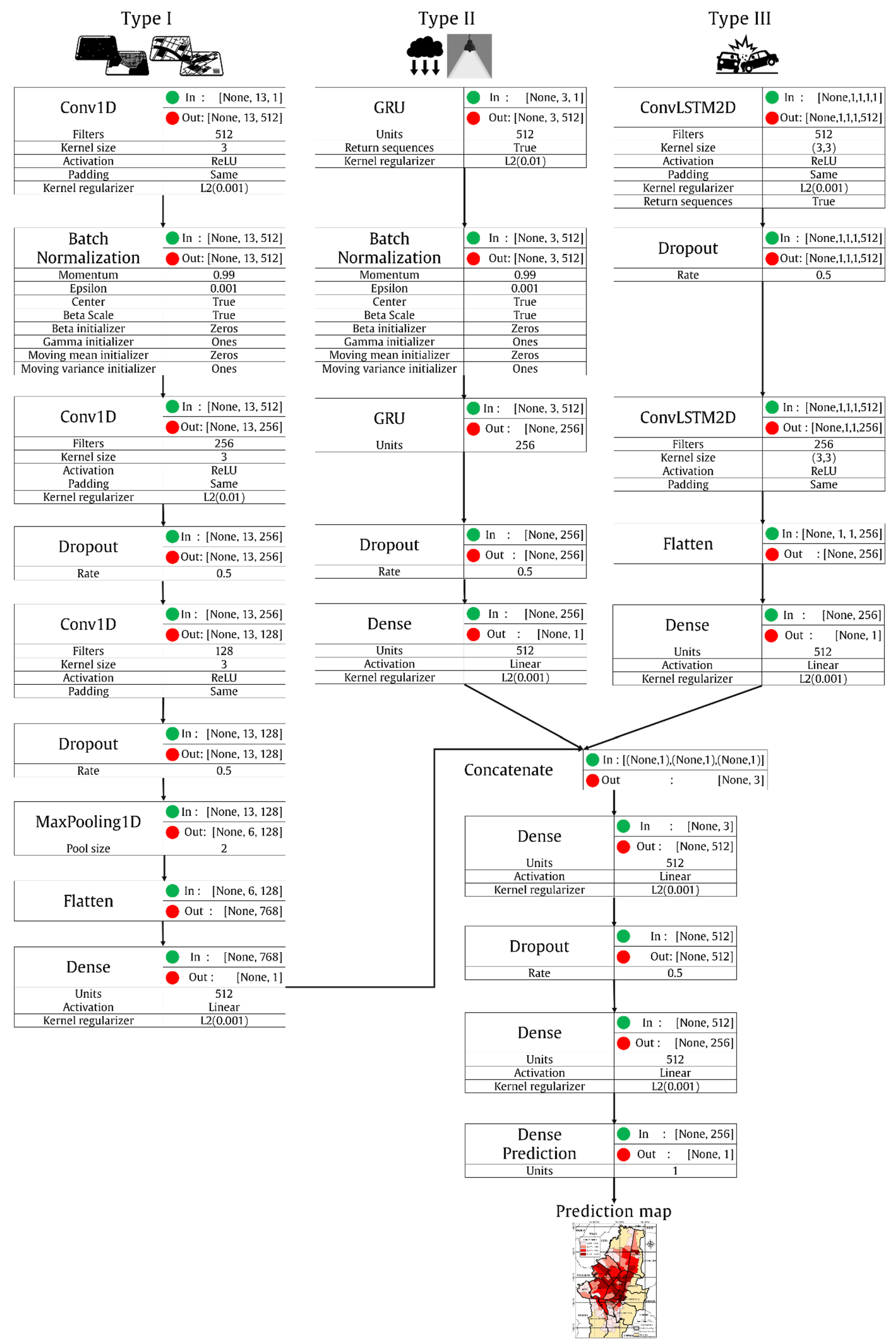
The SpatioConvGru-Net model is presented as a proposal to analyze traffic crashes as a time series in detailed hourly intervals, addressing the spatial and temporal correlation problem present in this phenomenon. Figure 2 shows the architecture of the proposed model built with the Python Tensorflow Framework v 2.16.

Figure 2. Architecture of proposed SpatioConvGru-Net model (Authors). The ’None’ notation used in the input and output dimensions of layers is a convention in frameworks such as TensorFlow/Keras to indicate a variable dimension, usually associated with the batch size. This dimension is defined dynamically during execution and does not imply the absence of data.

The inputs and layers that compose the submodels can be seen in Figure 2. The model uses three separate modules—CNN for spatial features, GRU for temporal patterns, and ConvLSTM for spatiotemporal dynamics—to align with the distinct nature of each data type. The CNN module captures static spatial dependencies from location-based variables such as socioeconomic, land use, and mobility indicators, which critically influence crash frequency. The GRU model learns the temporal patterns inherent to variables like precipitation and illumination that vary uniformly over time. Finally, ConvLSTM is included to model spatiotemporal data such as the crash index (TCIRP), which varies across both space and time. By preserving these separate extraction pipelines, the model leverages the strengths of each deep learning architecture while effectively capturing complex dependencies.

In the SpatioConvGru-Net model, the outputs are concatenated into a single feature vector. This combined representation is then passed through a series of fully connected dense layers that refine the information, applying regularization and non-linear transformations. The final dense layer uses a linear activation function to generate a unified prediction of traffic crash frequency. The submodels that compose the SpatioConvGru-Net are explained below.

The submodels that compose the SpatioConvGru-Net are explained below. Key training parameters included a batch size of 64, a maximum of 100 training epochs, and early stopping with a patience of 15 and a minimum delta of 0.0001. The model was optimized using the Adam optimizer with a learning rate adjustment per parameter, as further detailed at the end of this subsection.

2.3.1. Feature Engineering for Spatial Data Using CNN

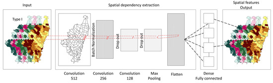
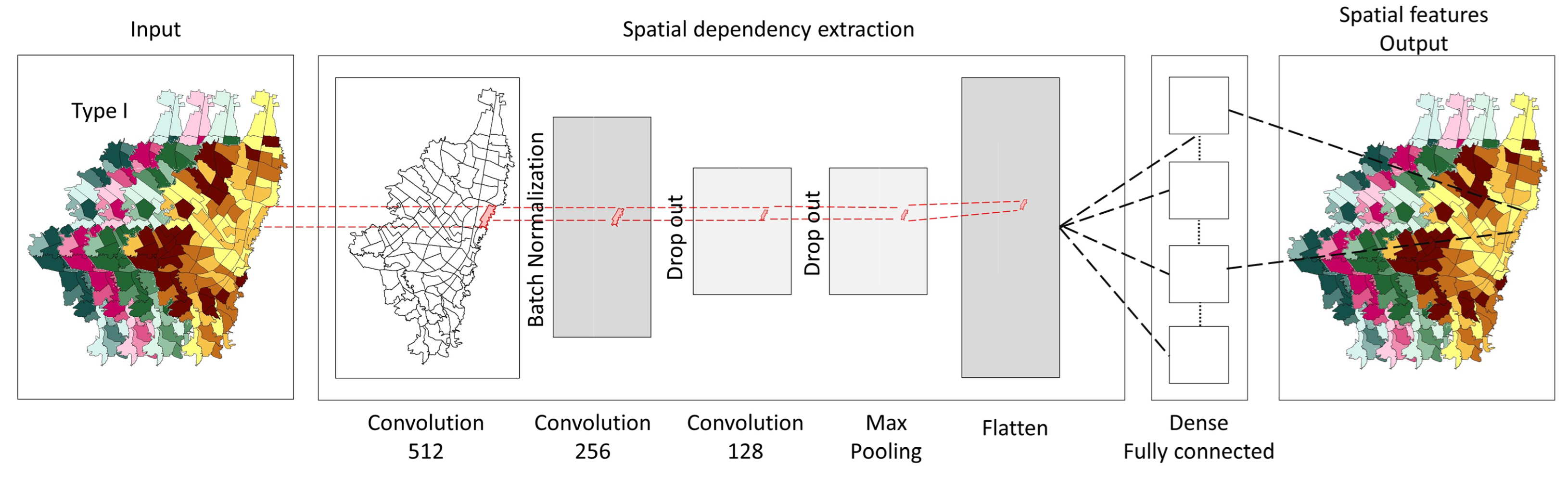
As [2,29] point out, CNNs are able to capture the inherent spatial dependency in traffic crash phenomena. A CNN was created to extract the spatial features of type I variables (see Figure 3).

Figure 3. CNN-based spatial feature extraction. Authors’ figure.

The input of the CNN is a vector with the values of the normalized type I variables for each spatial unit. Sequentially, the model applies a first convolution to extract the fundamental spatial patterns from the input data. Subsequent convolutions deepen the feature hierarchy, allowing the capture of more abstract and complex patterns in the data. Between these layers configured with 512, 256 and 128 filters of size 3, batch normalization and dropout elimination techniques are applied to improve model generalization and reduce overfitting [30]. Rectified Linear Units (ReLU) activation functions are used since in CNN they allow a faster learning rate with respect to the others [31,32]. The maximum clustering with a pool size of 2 is applied to reduce the spatial dimension of the learned features. The results are flattened into a one-dimensional vector and predictions are generated using a fully connected layer with a single output unit and a linear activation function.

2.3.2. Feature Engineering for Temporal Data Using GRU

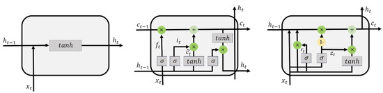
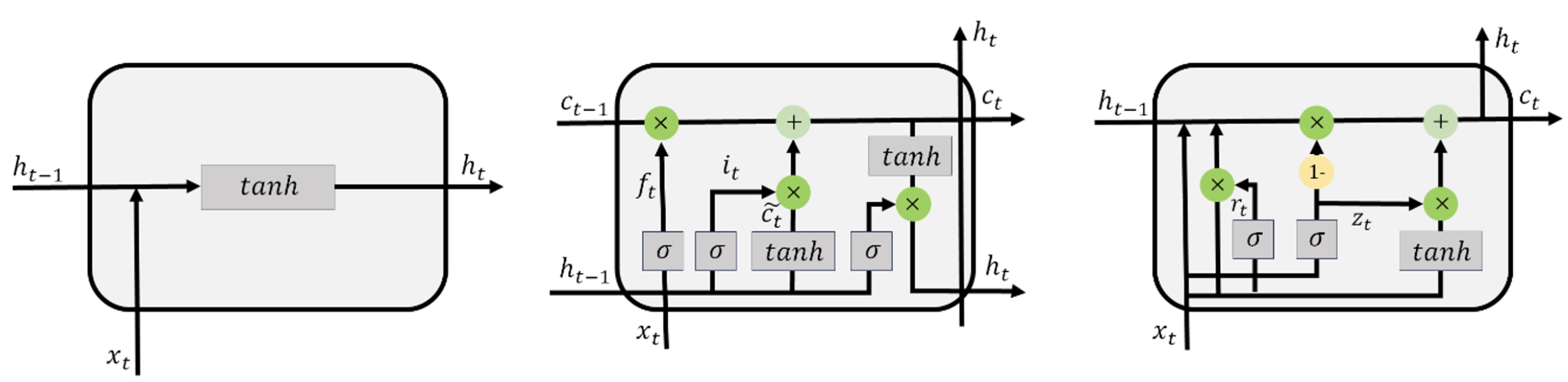
Unlike CNNs, several studies have shown that recurrent neural networks (RNNs) are efficient for feature extraction of data in time series structures [33,34]. Their efficiency is based on the ability to learn and retain prior information by processing data sequences in chronological order. This allows them to capture the temporal dependencies and discover complex patterns in the temporal evolution of data [35]. However, traditional RNNs have a problem called gradient fading or gradient explosion (gradients tend to become extremely small or large) that affects pattern learning and generalization in long-term sequential data [33,36,37]. To address this problem, there are specific RNNs such as LSTMs and GRUs (Figure 4).

Figure 4. Graphic illustration of simple Recurrent Neural Network (RNN) cell (on the left); Long-Short Term Memory (LSTM) cell (in the middle); Gated Recurrent Unit (GRU) cell (on the right). Authors’ figure.

LSTMs were introduced by [38] as a complex variant of RNN that, by incorporating memory gates that regulate the flow of information, allows the optimal learning of time series with long time periods. As an evolution of LSTMs, Ref. [39] proposed a simplified version called Gated Recurrent Units (GRUs), which offers improved network performance and requires less training time. These operate similarly to LSTMs, with the difference that the GRU cell uses a hidden state that merges the forgetting gate and the input gate into a single update gate. Therefore, the total number of gates in GRU is half the total number of gates in LSTM. In the following Equation (2) the hidden state $h_t$ of GRU is represented:

$$h_t=(1-z_t)·h_{t-1}+z_t·h_t$$

(2)

The update gate that determines which part of the GRU unit $z_t$ is updated is represented in the following Equation (3):

$$z_t=\sigma (W_z·[h_{t-1},X_t])$$

(3)

The restart gate $r_t$ is given by the following Equation (4):

$$r_t=\sigma (W_r·[h_{t-1},X_t])$$

(4)

The hyperbolic tangent function $h_t$ of the restart gate called New Recall Gate is described in the following Equation (5).

$$h_t=tanh(W·[r_t·h_{t-1},X_t])$$

(5)

where $\sigma$ is the sigmoid function; $X_t$ is the input at time t; $W_z$ is the weight matrix associated with the update gate and $W_r$ is the weight matrix associated with the reset gate.

For the present study, the GRU input is a vector with the precipitation variable normalized and the illumination variable hot-coded using OneHotEncoder. Sequentially, the model uses GRU layers configured with 512 and 256 units. The first layer oversees capturing the temporal patterns in the input data sequence, while the second layer processes the output sequence generated by the first layer. Batch normalization regularization is applied between these two layers. In addition, the Dropout technique is incorporated to improve the generalization of the model and avoid overfitting. Finally, a fully connected layer with a single output unit and linear activation function is applied to generate predictions.

In our experimental setup, both the LSTM and GRU architectures were evaluated under the same training conditions. Although LSTM has shown powerful performance in learning long-term dependencies, the GRU model achieved comparable accuracy while requiring fewer parameters and significantly less training time. Given the high spatiotemporal resolution of our dataset and the need to maintain computational efficiency across repeated model iterations (including transfer learning scenarios), GRU was selected as the optimal recurrent structure. Additionally, GRU’s simpler architecture helped mitigate the overfitting issues observed in preliminary tests with LSTM.

2.3.3. Spatiotemporal Features Extracted from ConvLSTM

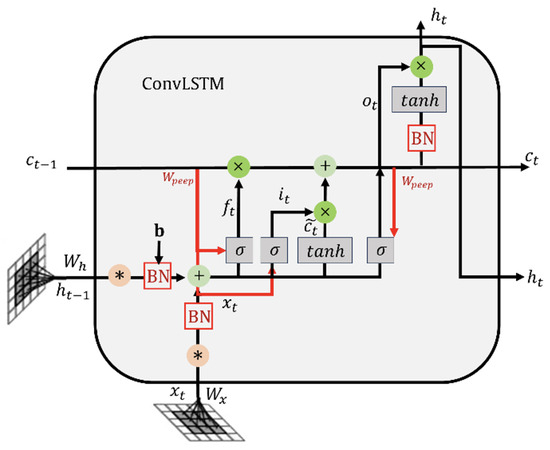
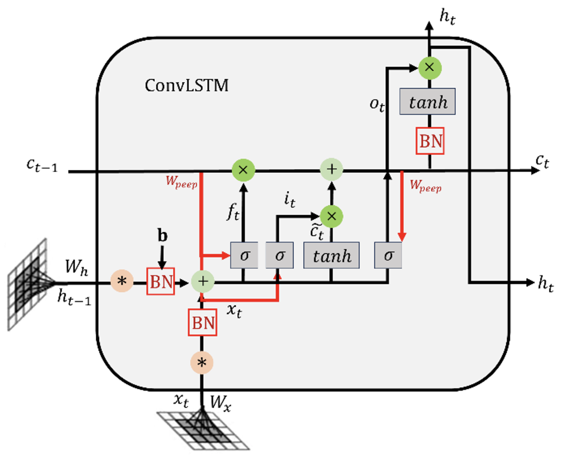
It has been expressed in previous sections how CNNs are able to extract spatial features, while RNNs are able to extract temporal features. However, neither can extract both simultaneously. Convolutional Long-Short Therm Memory (ConvLSTM) networks were introduced by [40] as a type of recurrent neural network that integrates concepts of convolutions and long-term memory for spatiotemporal prediction. It has convolutional structures in both input-to-state and state-to-state transitions. They have the facility to determine the future state of a given cell in the network through the inputs and past states of its local neighbors using a convolution operator at state-to-state and input-to-state transitions (see Figure 5).

Figure 5. Graphic illustration of Convolutional Long-Short Term Memory (ConvLSTM) (Authors).

where the input gate $i_t$ is represented by the following Equation (6):

$$i_t=\sigma (W_{xi}\ast X_t+W_{hi}\ast h_{t-1}+W_{ci}\odot C_{t-1}+b_i)$$

(6)

Oblivion’s gate $f_t$ is given by Equation (7):

$$f_t=\sigma (W_{xf}\ast X_t+W_{hf}\ast h_{t-1}+W_{cf}\odot C_{t-1}+b_f)$$

(7)

The memory cell $C_t$ is described in the following Equation (8):

$$C_t=f_t\odot C_{t-1}+i_t\odot tanh(W_{xc}\ast X_t+W_{hc}\ast h_{t-1}+b_c)$$

(8)

The output gate $o_t$ is represented by Equation (9):

$$o_t=\sigma (W_{x0}\ast X_t+W_{h0}\ast h_{t-1}+W_{c0}\odot C_{t-1}+b_0)$$

(9)

And the hidden state $h_t$ is represented by Equation (10):

$$h_t=o_t\odot tanh\left(C_t\right)$$

(10)

where $\sigma$ is the sigmoid function, $W_{hi}$ is the weight matrix associated with the input $X_t$. $W_{hi}$ is the weight matrix associated with the previous hidden state $h_{t-1}$. $W_{ci}$ is the weight matrix associated with the previous memory cell $C_{t-1}$. ⊙ is the Hadamart operator. * denotes the convolution operator. $C_{t-1}$ is the previous memory cell. $b_i$ is the bias associated with the input gate. The same case applies to the subscripts f, c, and o of the door of the oblivion gate, memory cell, and output gate.

According to the literature, in short-term traffic crash frequency prediction, ConvLSTM stands out as an outstanding choice that allows simultaneous spatial and temporal feature extraction [2,24,41]. In this study, the input of the ConvLSTM model receives a vector with the values of the normalized TCIRP variable. The first ConvLSTM2D layer with 512 filters performs convolution on temporal sequences, extracting complex spatiotemporal patterns, thanks to its ability to process data in both dimensions. The second ConvLSTM2D layer with 256 filters refines the representation obtained in the initial layer, further highlighting relevant features. In between these, L2 regularization and Dropout are applied to improve model generalization and avoid overfitting. The Flatten layer transforms the three-dimensional output into a one-dimensional vector, so that finally a Dense layer with a unit performs the final prediction.

2.3.4. Multimodal Fusion and Refinement

SpatioConvGru-Net employs a multimodal architecture that concatenates the spatial, temporal, and spatiotemporal features resulting from CNNs, LSTMs and ConvLSTMs into a single vector. This encapsulates the higher-level features related to socioeconomic, environmental land use and mobility variables. Sequentially, this vector serves as the input to the first dense layer that has 512 units and whose main function is to learn and represent complex features from the information coming from the three internal models. The second dense layer with 256 units continues the refinement process of the combined representation. Between these two layers, L2 regularization and Dropout are applied to improve model generalization and avoid overfitting. Both use the ReLU activation function that introduces nonlinearities in the output and allows learning more complex relationships in the data. The final dense layer has a single unit and linear activation that produces the predictions by averaging the model outputs computed by Equation (11):

$${\widehat{y}}_{SCTLSTM}=\left({\displaystyle \frac{W_{cnn}{X}_t^{cnn}+W_{lstm}{X}_t^{lstm}+W_{convlstm}{X}_t^{convlstm}}{3}}\right)+b_t$$

(11)

where $W_{cnn}$ and $X_t^{cnn}$; $W_{lstm}$ and $X_t^{lstm}$; $W_{convlstm}$ and $X_t^{convlstm}$ are the weights and features extracted by the CNN, LSTM and ConvLSTM at a time step t; b is the associated bias.

Although Equation (11) corresponds to a simple arithmetic average of the three base model outputs, this combination was selected after evaluating several alternative fusion strategies, including weighted averages and non-linear ensemble functions (e.g., logistic regression). The simple average demonstrated superior generalization capabilities and yielded the best validation performance across the experiments. Therefore, it was adopted as the final integration mechanism in this study.

2.3.5. Fine-Tuning with Transfer Learning for Small Areas

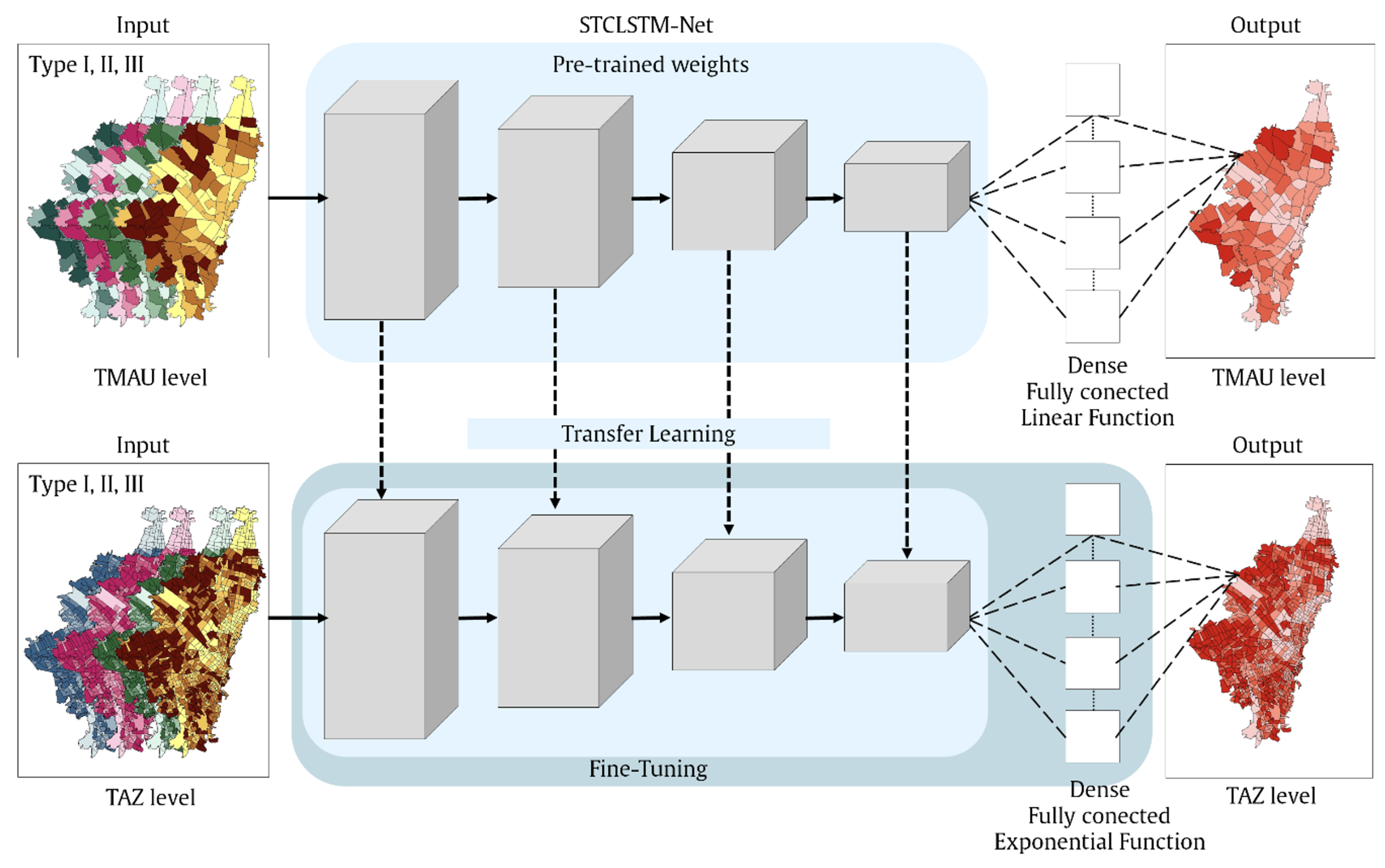
One of the challenges inherent in Deep Learning models lies in the ability to achieve effective generalization of their outputs in the presence of unseen data. This can be partially solved by using Transfer Learning (TL) techniques. These techniques consist of using a pre-trained model on a specific task and adapting or transferring its knowledge to a different but related task [42,43]. The idea is to leverage learning already conducted in one domain to improve performance in another. Fine-tuning (FT) is a TL-specific step that involves taking a pre-trained model and adjusting or tuning its weights on a specific task. In FT, some layers of the source (pre-trained) model are usually frozen to retain prior knowledge and remove the original fully connected layers to add another classifier, either by a fully connected layer or another classifier that allows feature extraction.

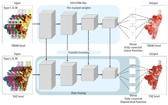
In this study, the source model SpatioConvGru-Net trained with the data at a geographic scale of TMAU was used to transfer knowledge and refine the weights on unseen data corresponding to a more detailed TAZ scale. For this the pre-trained weights of the source model were loaded, all layers are frozen, retaining the existing knowledge and three new fully connected layers are added with 2048, 1024 and 512 units. The activation function in these layers is ReLU. In the middle of these layers, Dropout is applied to improve the generalization of the model and avoid overfitting. Finally, a dense output layer with a single unit and exponential activation function is added to perform a Poisson regression given the excess of zeros in TAZ. The TL and FT process can be visualized in Figure 6.

Figure 6. Graphic representation of transfer learning and fine-tuning in the SCTLSM-Net model from TMAU to TAZ Level (Authors).

This approach is based on the literature, where it is established that strategies such as Transfer Learning and Fine-Tuning have the potential to improve the model performance in environments characterized by extreme imbalances, as is the case when spatiotemporal resolution is increased [44,45,46]. By virtue of the above and due to the limited effectiveness of the results when directly applying the original SpatioConvGru-Net model architecture to data at the TAZ scale, we chose to implement the Transfer Learning and Fine-Tuning strategy.

2.3.6. Training

In the compilation process, the loss function, optimizer, and evaluation metrics were configured to guide the training process of the SpatioConvGru-Net. The mean squared error (MSE) was used as the loss function. The Adaptive Moment Estimation (ADAM) optimizer was defined as matching the learning rate of each parameter individually [47] and whose weight update formula is defined in Equations (12)–(16).

$$m_t={\beta }_1·m_{t-1}+(1-{\beta }_1)·g_t$$

(12)

$$v_t={\beta }_2·v_{t-1}+(1-{\beta }_2)·g_t^2$$

(13)

$${\widehat{m}}_t={\displaystyle \frac{m_t}{1-{\beta }_1^t}}$$

(14)

$${\widehat{v}}_t={\displaystyle \frac{v_t}{1-{\beta }_2^t}}$$

(15)

$${\theta }_t={\theta }_{t-1}-\alpha ·{\displaystyle \frac{{\widehat{m}}_t}{\sqrt{{\widehat{v}}_t+ϵ}}}$$

(16)

$\theta$ are the model parameters (weights and biases), $\alpha$ is the learning rate. ${\beta }_1$ and ${\beta }_2$ are the decay factors of the moments. $g_t$ is the gradient of the loss function with respect to the time t parameters. $m_t$ and $v_t$ are the first and second order moments. ${\widehat{m}}_t$ and ${\widehat{v}}_t$ are the biased estimates of the moments. $ϵ$ is a small constant to avoid division by zero, and t is the iteration number. MSE, Mean Absolute Error (MAE) and Mean Absolute Percentage Error (MAPE) were set as evaluation metrics, (Equations (13)–(15)). The training was initialized to 100 epochs with a batch size of 64 and an early stopping monitoring the loss value metric with a maximum patience of 15 iterations and a minimum delta value of 0.0001. The development and training of the SpatioConvGru-Net was carried out using the Keras framework with Tensorflow as a backend. Experiments were conducted using Python 3.9 on a Linux cloud virtual machine with 1 SMP processor, 12 GB of RAM and a Tesla T4 graphics processing card with 15,360 MiB of memory.

Each training epoch took approximately 65 to 85 s, depending on the load distribution across batches. The training process concluded after 20 epochs due to the early stopping criterion being met, resulting in a total wall time of 27 min and 35 min of CPU time. These values demonstrate that the model achieves convergence in a reasonable computational window using accessible infrastructure. This efficiency highlights the feasibility of adopting the proposed methodology within institutional or municipal environments without requiring high-performance computing resources. This is particularly relevant for real-time or near real-time retraining scenarios where frequent model updates may be required to adapt to evolving urban dynamics.

Finally, although the general architecture of the model was adapted from a previously validated proposal [2], the specific hyperparameters used in the SpatioConvGru-Net were selected through a rigorous empirical tuning process. A hold-out validation set (20% of the training data) was used to guide the adjustment of training configurations, including batch size (64), number of epochs (up to 100), and optimizer settings. Training behavior was monitored using the validation loss curves and evaluation metrics (MSE, MAE, MAPE), ensuring that overfitting was avoided while optimizing generalization. Two monitoring mechanisms were integrated during training: the EarlyStopping callback (patience = 10, min_delta = 0.0001), which stopped training once convergence was detected, and the ModelCheckpoint callback, which stored only the model weights corresponding to the best validation loss. Although no automated hyperparameter optimization algorithm (such as grid search or Bayesian methods) was applied, the manual tuning process was based on quantitative evidence and ensured stability and robustness in model performance.

2.3.7. Evaluation

To evaluate the predictive performance of the SpatioConvGru-Net, the MSE, MAE, MAPE and R² metrics were used, which are calculated as follows (Equations (17)–(20)):

$$MSE={\displaystyle \frac{1}{n}}\sum _{i=1}^n{(y_i-{\widehat{y}}_i)}^2$$

(17)

$$MAE={\displaystyle \frac{1}{n}}\sum _{i=1}^n|y_i-{\widehat{y}}_i|$$

(18)

$$MAPE={\displaystyle \frac{1}{n}}\sum _{i=1}^n{\displaystyle \frac{|y_i-{\widehat{y}}_i|}{y_i}}\times 100$$

(19)

$$R^2=1-{\displaystyle \frac{{\sum }_{i=1}^n{(y_i-{\widehat{y}}_i)}^2}{{\sum }_{i=1}^n{(y_i-{\overline{y}}_i)}^2}}$$

(20)

where n is the total number of observations, $y_i$ the observed values, ${\widehat{y}}_i$ the predicted and ${\overline{y}}_i$ the mean of observed values. In addition, the metrics obtained were compared with classical econometric, machine learning, and deep learning models used for similar purposes. According to the literature, [2,18,20,33,36], the most commonly used classical econometric methods have been the Moving Average Integrated Autoregressive (ARIMA) model [48] and Geographically Weighted Regression (GWR) [49]. While Gradient Boosting Regression Tree (GBRT), Convolutional Neural Networks (CNN) and Recurrent Neural Networks (RNN) models are the most common for this purpose [2,40,50]. Based on the above, these models were chosen as a reference for comparison with the proposed model.

3. Results

The results derived from the application of the proposed methods are presented below. Initially, an exploratory analysis of the study variables was performed, with a particular focus on the variables of interest. This was to provide a detailed understanding of the distribution and behavior of each variable considered, highlighting the relevance and particularities associated with the variables of interest in the general context of the study. Consequently, a comparison is made with the results obtained through conventional approaches to evaluate the effectiveness and validity of the proposed methodology in achieving the established objectives. This analysis is based on statistical rigor and technical interpretation of the findings, providing a solid basis for conclusions and subsequent recommendations.

3.1. Preparation and Exploration Data Analysis

First, the latent variable land use and socioeconomic stratification (LU_ST) constructed from the individual contributions of each nominal variable was generated through a multiple correspondence analysis (MCA). This composite variable has a positive impact on traffic crash frequency [13]. The construction of the variable is described in Equation (21).

$$LU\_ST=\sqrt{{\sum }_{i=1}^{n=6}{\left({\displaystyle \frac{Di{m}_i\times {\sigma }_{E_i}}{{\sigma }_T}}\right)}^2}$$

(21)

where i is the i-th dimension; ${\beta }_i$ is the percentage of variance explained in dimension i and $\gamma$ is the total percentage of variance explained in n dimensions. With this latent variable, a data set composed of fifteen (15) independent variables and the variable of interest, TCIRP, was consolidated. Table 3 and Table 4 show the descriptive statistics corresponding to the response variable and its covariates used in the framework of this research.

Table 3. Descriptive statistics at TMAU level *.

Variable	Name	Mean	Median	S.D.	Min	Max	Kurt	Skew	V.C.
	Land use factors
LU_ST	Land uses & Socioeconomic stratification	0.60	0.59	0.30	0.29	1.78	0.92	0.99	49.84
	Socioeconomical Factors
PD	Population density	18,963.10	19,553.30	11,538.55	0	53,668.60	4.67 × 103	0.43	60.85
RMMV	Rate of motorization of motor vehicles	236.60	212.46	139.03	0	753.43	1.24	1.09	58.76
NH	Number of households	19,411.18	15,936.50	14,959.57	0	85,108.00	2.63	1.31	77.07
	Mobility factors
RPTP	Rate of pedestrian trips per person	8.88 × 102	8.93 × 102	1.50 × 102	0	1.16 × 101	19.54	−3.56	16.92
RTPPT	Rate of trips per person in public transport	2.44 × 102	2.51 × 102	7.58 × 103	0	4.39 × 102	1.53	−0.77	31.00
RTPT	Rate of trips per person by taxi	4.26 × 103	3.25 × 103	2.96 × 103	0	1.23 × 102	−0.19	0.80	69.42
RTPC	Rate of trips per person by car	1.39 × 102	1.12 × 102	1.18 × 102	0	6.27 × 102	1.59	1.26	85.01
RTPM	Rate of trips per person on motorcycle	3.32 × 103	3.30 × 103	1.82 × 103	0	1.03 × 102	1.38	0.89	54.77
RTPB	Rate of trips per person by bicycle	4.02 × 103	3.48 × 103	2.71 × 103	0	1.37 × 102	0.76	0.90	67.37
TTDOD	Trips in a typical day origin-destination	9517.41	8440.91	6254.29	46.00	32,909.30	1.67	1.18	65.71
TRPTM	Travel rate per person in BRT system	0.19	6.51 × 102	0.46	0	4.29	55.52	6.86	246.42
AMSA	Average maximum speed allowed	38.88	38.61	6.00	30.27	56.50	0.24	0.87	15.44
	Environmental factors
PCP	Precipitation	3.70 × 102	0	0.45	0	21.60	926.60	25.85	1203.01
ILLUM	Illumination	—	—	—	—	—	—	—	—
	Response variable
TCIRP	Traffic Crashes Index on the road perimeter	5.31 × 104	0	3.72 × 103	0	1.48 × 101	213.03	11.43	700.59

* Note: Descriptive statistics are computed from TMAU-level data. “—” indicates missing data.

Table 4. Descriptive statistics at TAZ level *.

Variable	Name	Mean	Median	S.D.	Min	Max	Kurt	Skew	V.C.
	Land use factors
LU_ST	Land uses & Socioeconomic stratification	0.58	0.45	0.33	0.29	1.83	1.46	1.44	56.86
	Socioeconomical Factors
PD	Population density	2386.66	1788.78	2388.28	0	19,364.71	9.84	2.59	100.07
RMMV	Rate of motorization of motor vehicles	29.78	19.57	35.35	0	405.99	33.19	4.62	118.72
NH	Number of households	2443.04	1862.50	2251.64	0	19,314.00	9.70	2.42	92.17
	Mobility factors
RPTP	Rate of pedestrian trips per person	1.12 × 102	8.79 × 103	9.57 × 103	0	0.10	17.66	3.22	85.59
RTPPT	Rate of trips per person in public transport	3.08 × 103	2.29 × 103	2.85 × 103	0	3.36 × 102	27.45	3.75	92.66
RTPT	Rate of trips per person by taxi	5.37 × 104	3.57 × 104	6.02 × 104	0	4.66 × 103	13.08	3.08	112.10
RTPC	Rate of trips per person by car	1.75 × 103	9.12 × 104	2.70 × 103	0	3.65 × 102	56.70	6.04	153.82
RTPM	Rate of trips per person on motorcycle	4.18 × 104	2.96 × 104	4.98 × 104	0	8.60 × 103	89.27	6.91	119.09
RTPB	Rate of trips per person by bicycle	5.06 × 104	3.27 × 104	5.68 × 104	0	5.19 × 103	14.37	3.12	112.22
TTDOD	Trips in a typical day origin-destination	1197.84	931.27	966.96	4.26	6907.87	5.34	1.90	80.73
TRPTM	Travel rate per person in BRT system	2.35 × 102	7.59 × 103	7.95 × 102	0	1.46	188.27	12.42	338.74
AMSA	Average maximum speed allowed	38.44	36.62	7.59	30.00	60.00	0.24	0.97	19.74
	Environmental factors
PCP	Precipitation	3.68 × 102	0	4.43 × 101	0	21.60	926.68	25.83	1203.94
ILLUM	Illumination	—	—	—	—	—	—	—	—
	Response variable
TCIRP	Traffic Crashes Index on the road perimeter	5.39 × 104	0	1.17 × 102	0	2.59	2510.65	39.13	2177.57

* Note: V.C. refers to Variation Coefficient expressed as a percentage. Data analyzed at the Traffic Analysis Zone (TAZ) level.

The statistics reflect the significant differences in the TCIRP response variable between the TMAU and TAZ levels. For both spatial units, the coefficient of variation (V.C.) shows that there is wide data dispersion. This is more pronounced at the TAZ level compared to TMAU, suggesting greater heterogeneity of the TCIRP as the spatial unit becomes smaller. Regarding the TCIRP distribution, for both units, a concentration and bias to the right is observed, with a concentration of values close to zero and more accentuated at the TAZ level, because as the scale becomes more detailed, the aggregate counts per spatial unit decrease. The variability in the TCIRP is lower at the UTAM level, whose range goes from 0 to 0.148; at the TAZ level, the range extends from 0 to 0.259, reflecting a greater variability and amplitude in the distribution of traffic crashes.

Furthermore, the descriptive statistics of the explanatory variables reveal substantial asymmetries across spatial units. At the TAZ level, higher skewness and kurtosis are observed for multiple predictors—such as motorization rate, trip rates by transport mode, and population density—indicating the presence of heavy-tailed distributions and extreme values. These patterns are consistent with the urban heterogeneity and localized behaviors observed in finer-scale zones. Such statistical characteristics underscore the importance of normalization steps and justify the inclusion of robust evaluation metrics. Specifically, the overdispersion and zero-inflation of the TCIRP variable—especially at the TAZ level—support the use of count-sensitive metrics such as the Poisson deviance in addition to standard regression measures.

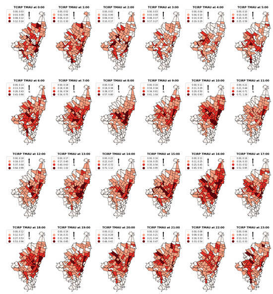
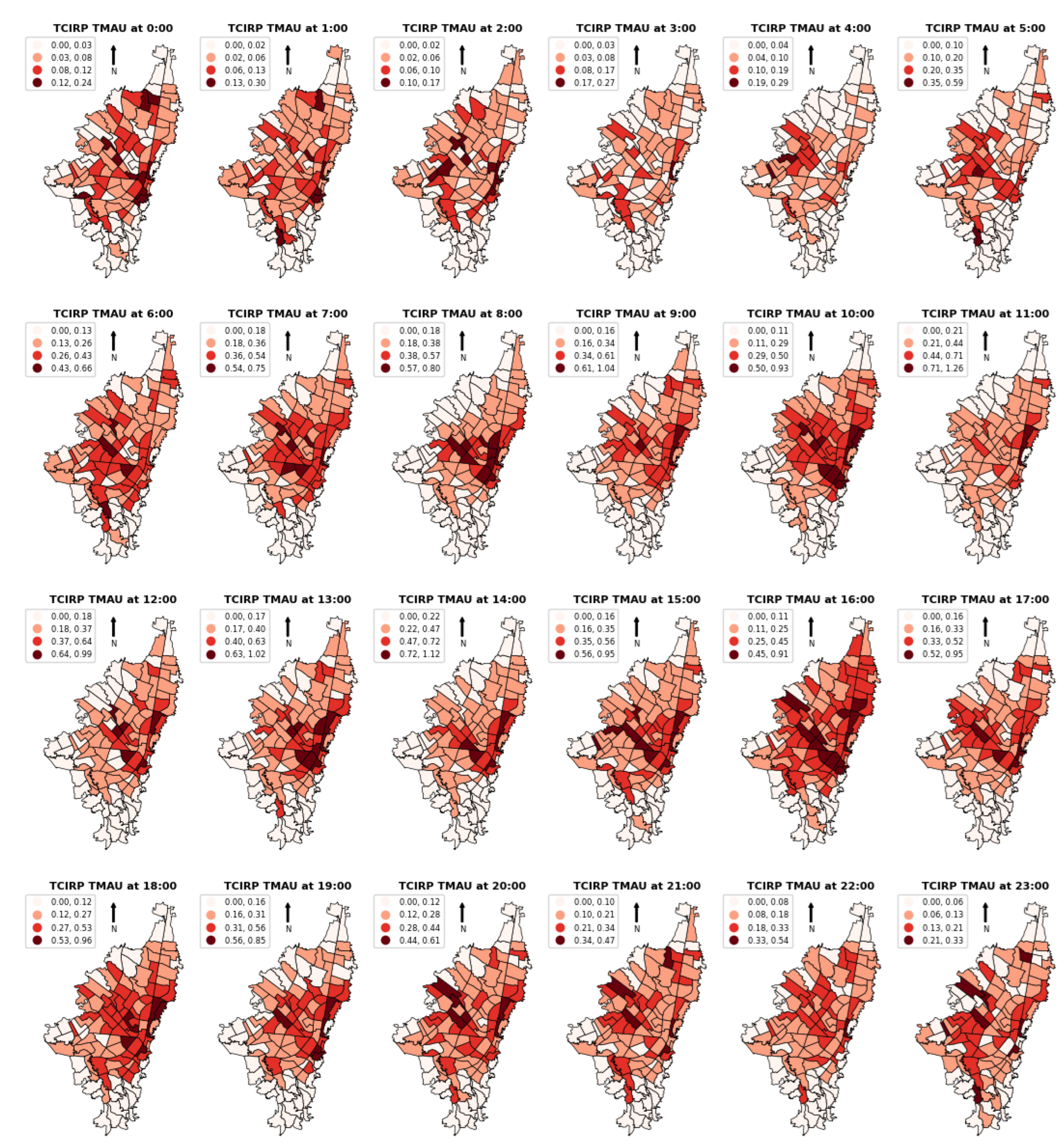
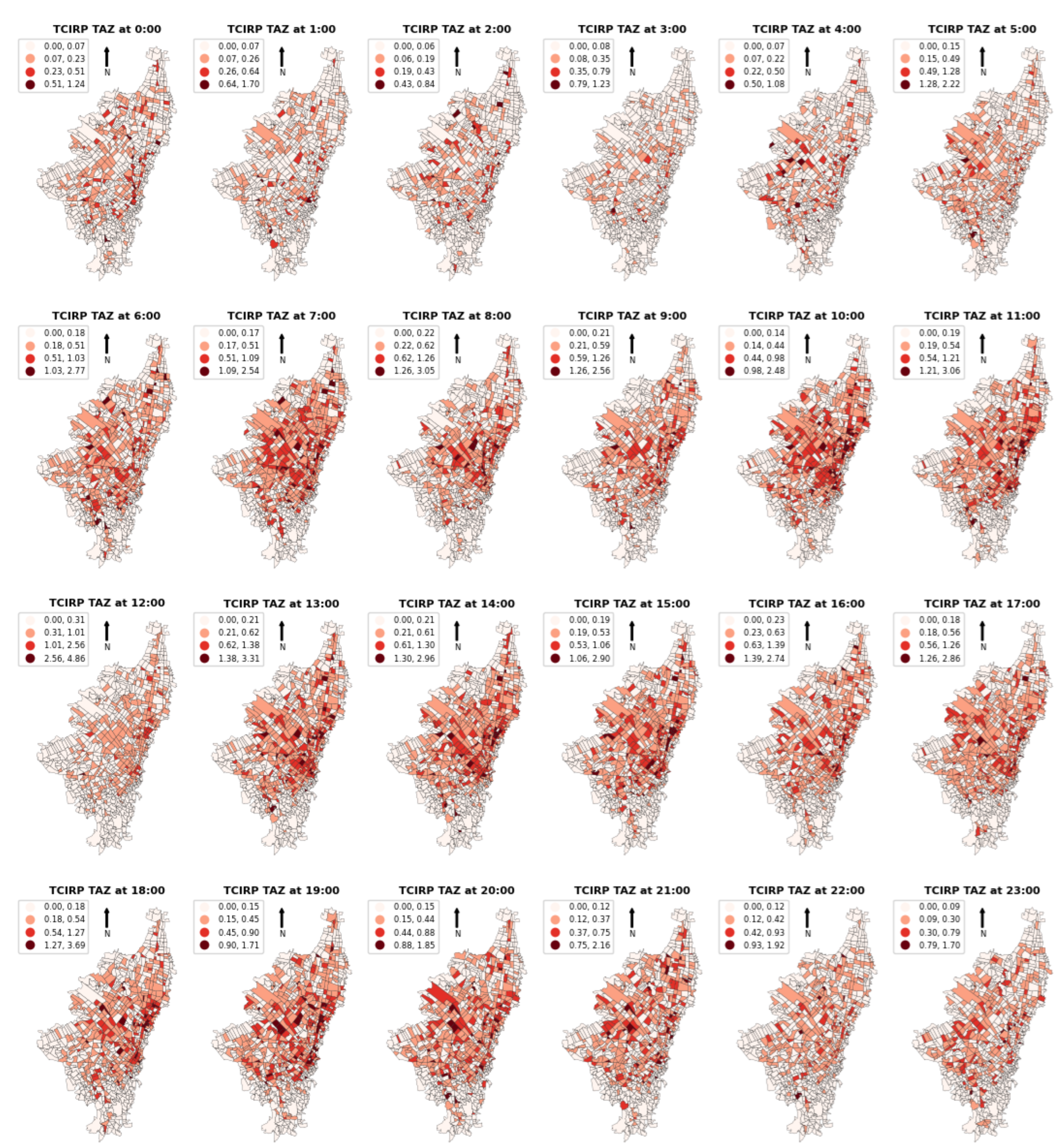
It is evident that the time of the traffic crashes in 2019 shows that the highest values of traffic crashes are concentrated in the time interval between 6:00 and 20:00 (See Figure 7 and Figure 8). In this time range there are peak values at 7:00, 13:00 and 14:00 whose counts amount to 1769, 1851 and 1961, respectively. In contrast, the values begin to decrease in the range of the night and early morning, where the minimum value of counts is drastically reduced to 256 at 3:00.

Figure 7. Spatial Distribution of TCIRP at TMAU Level: Hourly variation in the study area using natural breaks classification (Authors).

Figure 8. Spatial distribution of TCIRP at TAZ Level: Hourly variation in the study area using natural breaks classification (Authors).

Figure 7 shows the spatial distribution of the TCIRP at the TMAU level, where the spatial clusters formed by high and low values at the hourly level can be clearly differentiated. In addition, the highest TCIRP value (1.26) occurs at 11:00.

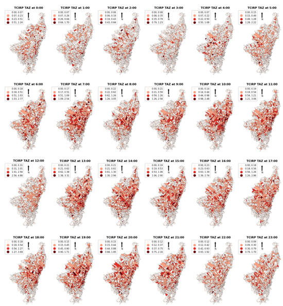
Similarly, Figure 8 shows the spatial distribution of the TCIRP at the TAZ level at the quartile level. In the time range from 0:00 to 4:00, the minimum value of 0 predominates in most of the units. The highest TCIRP value (4.86) occurs at 12:00.

3.2. SpatioConvGru-Net Results

For this study, we proposed two short-term hourly traffic crash prediction models at different spatial resolutions: TMAU (origin) and TAZ (detailed). The origin model was trained, evaluated, and validated with the totality of the TMAU spatial units in the period from 1 January to 31 December 2019. Similarly, we calculated the detailed model (TL+FT) with all the TAZ spatial units. The sample size per spatial unit for each traffic crash prediction model is shown in Table 5.

Table 5. Sample size for spatial unit prediction models. All models were trained, validated, and tested using the same temporal data split (1 January–13 September 2019 for training; 14 September–9 October 2019 for validation and 10 October–31 December 2019 for testing).

Spatial Unit	Sample Size	Training Sample	Testing Sample	Evaluation Sample	Spatial Units	Average Area (Km2)
TMAU	963,600	674,520	192,720	96,360	110	3.67
TAZ	7,656,240	5,359,368	1,531,248	765,624	874	0.46

For each model the selected data set was divided into a training, test, and validation set in a proportional ratio 70%, 20% and 10%. The training dataset spanned from 1 January to 13 September 2019; the validation dataset spanned from 14 September to 9 October 2019 and the test dataset spanned from 10 October to 31 December 2019. This partitioning strategy was applied uniformly across all models to ensure consistency in training, validation, and testing.

Figure 7 and Figure 8 illustrate the temporal variation in TCIRP in 2019 in Bogota. Furthermore, we can see that the data sets (training, test, validation) exhibited both high and low values of TCIRP, reflecting a balanced distribution of traffic crashes at their extremes of occurrence.

The results of the proposed SpatioConvGru-Net and other models tested for short-term traffic crashes prediction can be seen in Table 6. The MSE and MAPE metrics on unobserved data (validation) indicate an approximate 94% reduction in the TMAU level with respect to TAZ. Likewise, the MAE experiences an approximate 65.5% deterioration at the more detailed level. Nevertheless, the coefficient of determination in TAZ exceeded 68%, suggesting an acceptable predictive performance at this geographic level. A comparative analysis of the metrics exhibited a decrease in the predictive performance of the model as spatial resolution increased. This trend was consistent with expectations, since prediction in smaller areas became more complex as the probability of occurrence of random events tended to decrease with increasing level of detail at the spatial scale.

Table 6. Comparative assessment of model performance *.

TMAU
	Training					Testing					Validation
Models	MSE	MAE	MAPE	R2	PD	MSE	MAE	MAPE	R2	PD	MSE	MAE	MAPE	R2	PD
SpatioConvGru-Net	0.018	0.023	5.54	0.982	0.026	0.018	0.022	5.50	0.981	0.027	0.017	0.023	5.54	0.983	0.025
CNN	0.036	0.033	7.07	0.852	0.058	0.039	0.035	7.07	0.851	0.059	0.041	0.040	7.08	0.841	0.060
LSTM	0.028	0.025	6.32	0.889	0.044	0.032	0.026	6.33	0.887	0.046	0.034	0.028	6.34	0.880	0.045
GRBT	0.038	0.038	7.45	0.842	0.056	0.041	0.041	7.46	0.839	0.057	0.040	0.045	7.46	0.813	0.058
ARIMA	0.037	0.027	7.09	0.874	0.048	0.036	0.025	7.07	0.871	0.047	0.038	0.029	7.08	0.853	0.049
GWR	0.051	0.043	8.00	0.828	0.065	0.054	0.046	8.12	0.813	0.066	0.052	0.055	8.13	0.796	0.067
TAZ
	Training					Testing					Validation
Models	MSE	MAE	MAPE	R2	PD	MSE	MAE	MAPE	R2	PD	MSE	MAE	MAPE	R2	PD
SpatioConvGru-Net	0.032	0.067	99.74	0.690	0.062	0.029	0.065	99.77	0.683	0.061	0.032	0.067	99.74	0.687	0.063
CNN	0.042	0.077	101.79	0.582	0.078	0.046	0.079	101.79	0.572	0.079	0.044	0.077	101.79	0.569	0.077
LSTM	0.046	0.071	100.98	0.601	0.074	0.045	0.074	100.99	0.595	0.075	0.046	0.073	100.98	0.583	0.076
GRBT	0.043	0.075	101.47	0.573	0.076	0.048	0.081	101.47	0.569	0.078	0.045	0.079	101.47	0.561	0.077
ARIMA	0.042	0.075	100.63	0.592	0.075	0.042	0.082	100.64	0.589	0.076	0.042	0.080	100.63	0.580	0.075
GWR	0.048	0.089	101.98	0.529	0.080	0.049	0.090	101.98	0.501	0.082	0.048	0.091	101.98	0.499	0.081

* SpatioConvGru-Net shows the best performance across all metrics in both TMAU and TAZ datasets.

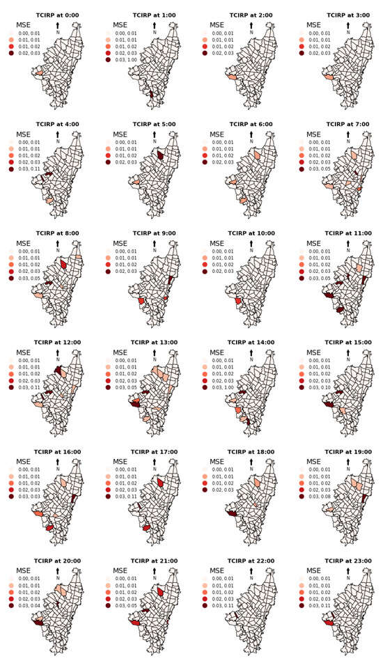
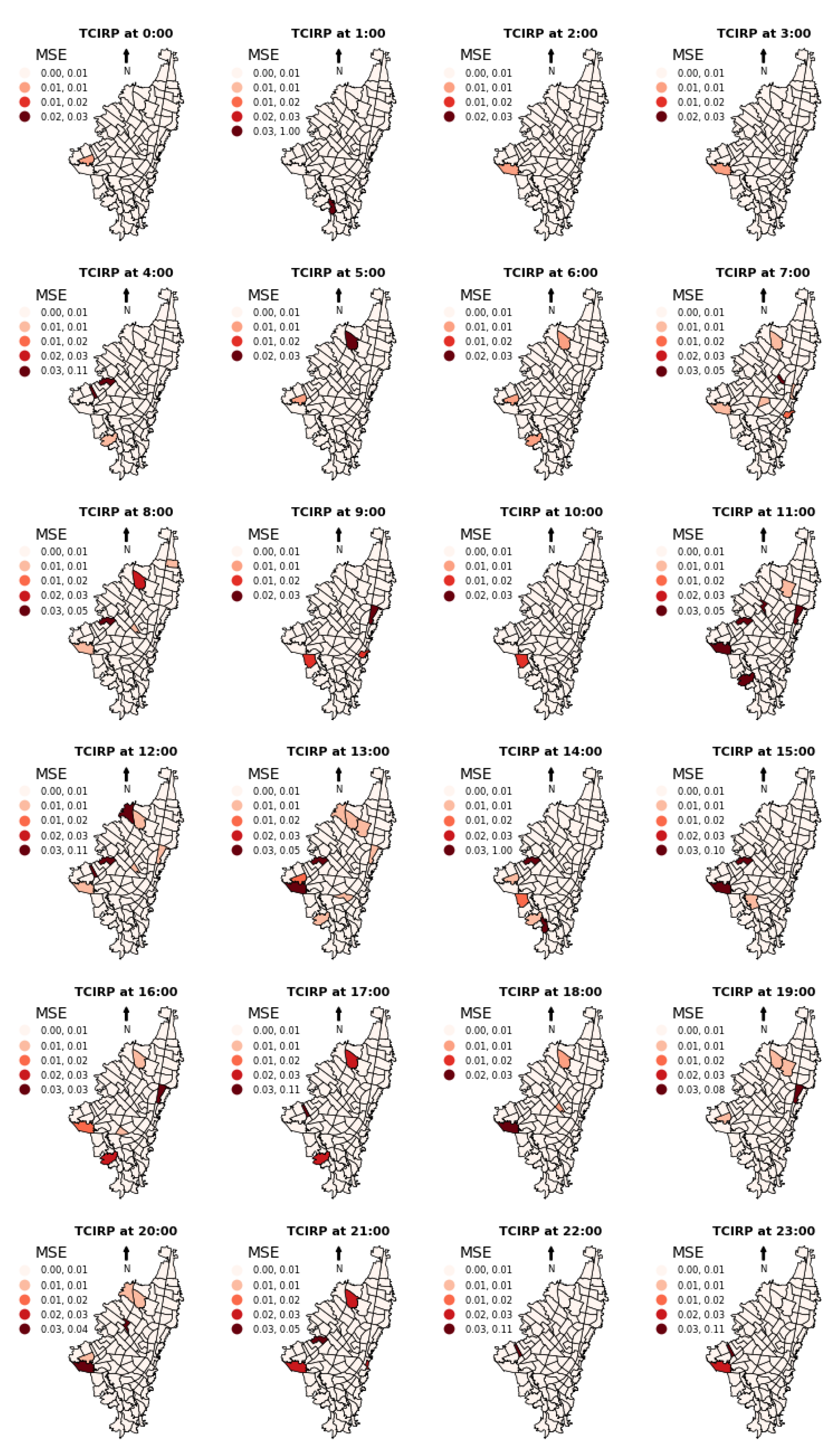
Figure 9 and Figure 10 show the error for the predicted values of the TCIRP at the TMAU and TAZ levels. Generally, at the TMAU level, the model was able to predict the TCIRP with great accuracy, even in the areas with the highest level of traffic crashes. Specifically, during the hours between 7:00 and 14:00, characterized by a higher traffic crash rate, the model presented an accurate prediction in the identification of low, medium, and high levels of TCIRP. However, it had limitations in that it was not able to accurately predict the highest range of TCIRP values during the 1:00 to 4:00 h.

Figure 9. MSE for predicted values of TCIRP with the validation dataset at TMAU level (Authors).

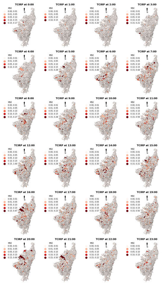
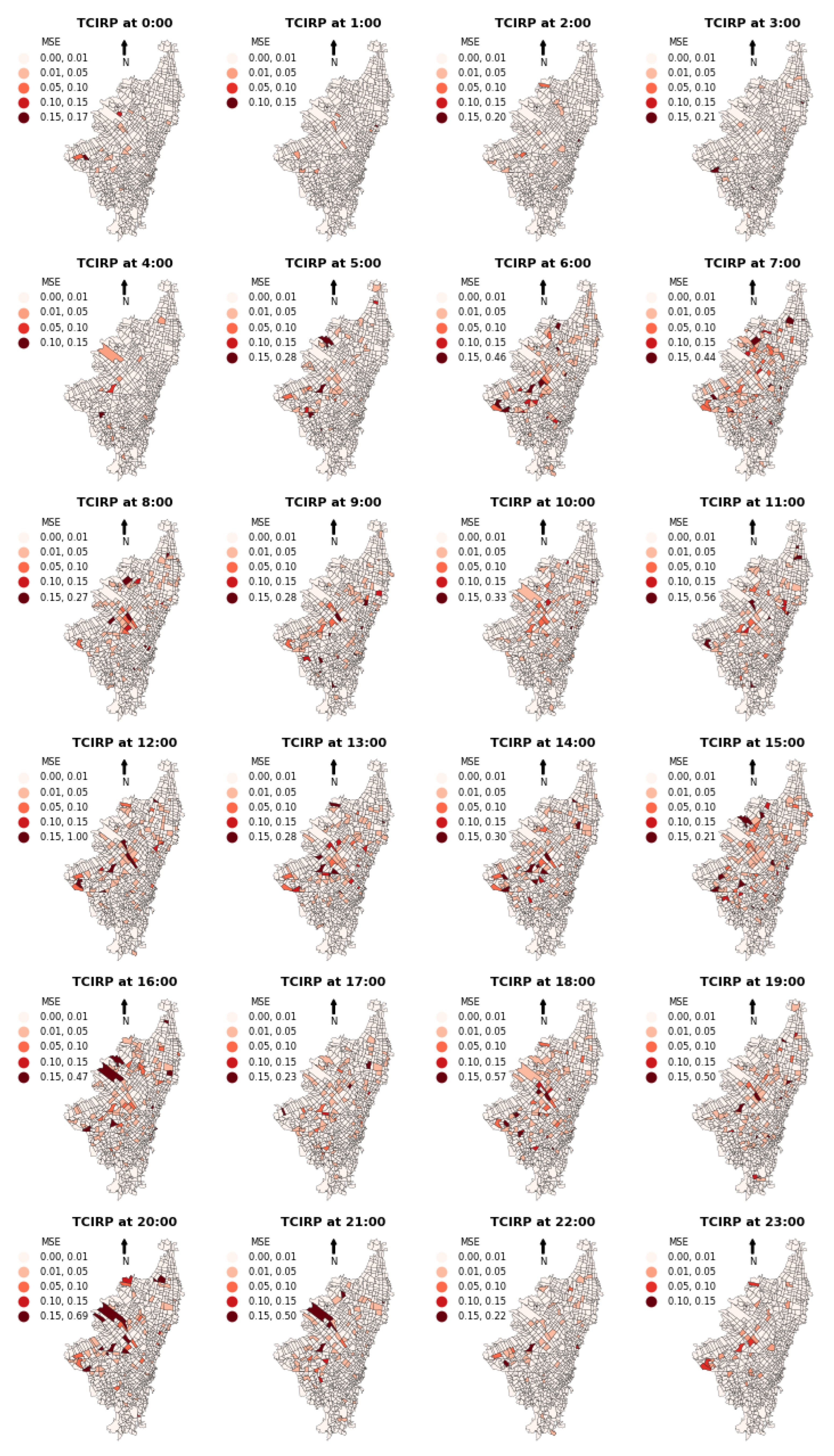
Figure 10. MSE for predicted values of TCIRP with the validation dataset at TAZ level (Authors).

In contrast, and as expected at the TAZ level, accuracy decreased since the model was not able to predict the high values of TCIRP. Despite the acceptable performance in predicting low and medium TCIRP values, the model exhibited significant limitations in the higher ranges. This was mainly noticeable in the 11:00, 12:00 and 19:00 time slots, where the predicted maximum values barely matched the observed mean TCIRP levels. Therefore, despite having an acceptable coefficient of determination, it was important to note that this was mainly attributed to the recognition of areas where the occurrence of traffic crashes was moderate, low, or null.

3.3. Evaluating Model Performances

The performance evaluation of the proposed model was conducted by comparing it with classical econometric models, machine learning, and deep learning models that have been used to predict traffic crashes as time series. The same training, evaluation, and validation data set was used in the ratio 70:20:10 with the time intervals indicated in Section 2. The only difference is that the SpatioConvGru-Net model received as input the three different types of data, while in the others, there was only a single input corresponding to the matrix of exogenous variables. The results of the evaluation metrics are shown in Table 6.

In a top-down manner based on the MSE, MAE and MAPE, the SpatioConvGru-Net model has the best metrics, followed by the LSTM, CNN, GBRT, ARIMA and GWR. The above agrees with previous studies where deep learning methods such as CNN and LSTM outperform classical regression models in predictive performance [2,36]. However, we observed that the classical models do not show a significant gap with respect to the GBRT machine learning model. This may be mainly because models such as ARIMA and GWR may be more appropriate for capturing spatial variation [51]. In the totality of the cases analyzed, we observed that the metrics at the TMAU level consistently showed superior performance with respect to those obtained at the TAZ level. This finding was consistent with the literature, since as spatial resolution increases, the increasing complexity of spatial relationships tends to cause a decrease in predictive performance [2,13,22]. This could also be attributed to the bias towards zero in the models, since as the spatial resolution increases, the probability of occurrence of traffic crashes tends to decrease and the counts per spatial unit assimilate to a negative binomial distribution [6]. The results proved that the SpatioConvGru-Net model exhibited significantly superior performance compared with previously implemented models for short-term traffic crash prediction. This may be because, on the one hand, classical econometric models lack capabilities to simultaneously address the spatiotemporal dependency problem, while individual deep learning models such as the CNN model do not exhibit optimal performance in capturing temporal dependencies and the LSTM exhibits limitations in addressing the spatial dependency problem [2]. The above shows the effectiveness of integrating specialized models for specific tasks, taking advantage of their capabilities to capture in parallel complex relationships that they were not originally designed to address. The above considerations allowed demonstrating that the proposed SpatioConvGru-Net model was a highly effective option to predict traffic crashes in a very detailed temporality at hourly levels and in relatively large spatial units such as zonal planning units that have characteristics of homogeneous socioeconomic, demographic, and economic destinations. Finally, it is important to highlight that the architecture of the proposed model was the result of multiple experiments modifying the models by data type, finding that in this case, the simplified RNN GRU model of the LSTM was more effective for capturing time dependence. Likewise, using strategies such as transfer learning and fine-tuning is very useful to find the best model when it is not possible to obtain acceptable results with direct training on the sample in question. To conclude, it is imperative to highlight that, given the complexity and the volumetric nature of the hyperparameters that characterize this type of model, it is necessary to use regularization methodologies to mitigate overfitting and improve the generalization capacity of the model.

Despite the differences in spatial granularity, the SpatioConvGru-Net model demonstrated coherent predictive performance across both levels of spatial aggregation. Specifically, while the model achieved higher accuracy in the TMAU level (R² = 0.981, MAE = 0.022), its performance at the TAZ level remained stable and acceptable (R² = 0.683, MAE = 0.065). This consistency indicates the model’s robustness and adaptability when handling heterogeneous spatial units and confirms the feasibility of applying the approach to different levels of aggregation in urban contexts.

4. Discussion

The results of this study demonstrate that the SpatioConvGru-Net model constitutes an effective tool for the short-term spatiotemporal prediction of traffic crashes in complex urban environments. However, several methodological aspects and limitations require consideration within the framework of this research.

4.1. Model Performance and Spatiotemporal Patterns

The proposed model exhibited superior performance compared to classical econometric, machine learning, and deep learning methods. At the TMAU level, notable accuracy was achieved (R² = 0.983, MSE = 0.017, MAPE = 5.5%), effectively capturing the crash intensity patterns during peak hours and along main corridors. This superiority is attributed to the hybrid model’s capability to simultaneously address spatial, temporal, and spatiotemporal dependencies inherent to the phenomenon.

Temporal analysis revealed that crash intensity is primarily concentrated between 6:00 and 20:00 h, with characteristic peaks at 7:00, 13:00, and 14:00. Spatially, central zones and main arteries show higher risk during commuting periods, while peripheral areas present more stable patterns.

4.2. Spatial Resolution Challenges

As spatial resolution increases (from TMAU to TAZ), an expected degradation in predictive performance is observed. The model experiences systematic difficulties in predicting extreme high-intensity events, especially during 11:00–12:00 h, where notable underestimation occurs in short segments with rare but intense events. This limitation reflects the inherent zero-bias in data when the probability of crash occurrence decreases in smaller spatial units.

The implementation of transfer learning and fine-tuning proved effective for improving performance at detailed scales, achieving a 4% improvement in evaluation metrics. Although this increase was not evaluated through formal statistical tests, in the context of complex deep learning architectures with high baseline accuracy, even small relative gains are considered significant.

4.3. Methodological Limitations

The proposed TCIRP index as the variable of interest may not fully represent the general phenomenon of traffic crashes, as it depends mainly on the total length of kilometers contained in each zone. In areas with limited road infrastructure, the index may be inflated due to a very small denominator. Also, the study uses 2019 data, which represent the most complete and reliable period prior to the COVID-19 pandemic. While this may limit direct generalization to current conditions, the model is designed to be easily retrainable with updated datasets.

The model was not designed to discriminate the individual impact of explanatory factors on traffic crashes. Variables were selected based on prior empirical evidence, and regularization techniques were applied to mitigate multicollinearity risks.

4.4. Implications for Urban Management

The findings have direct implications for urban road safety management:

• Risk area anticipation: Identification of zones with higher crash probability facilitates implementation of preventive measures and resource allocation.
• Emergency resource planning: Accurate predictions enable advanced planning and optimization of response in case of crashes.
• Traffic policy development: Results can inform long-term policies, including infrastructure planning and road safety measures.
• Associated cost minimization: Crash prediction can reduce the costs of emergency care, infrastructure repair, and compensation.

4.5. Future Directions

For future research, we recommend:

• Integrating econometric models with zero-inflated components (Zero-Inflated Hurdle Model, Zero-Inflated Mixed Effects Model)
• Exploring attention-based architectures (Transformer blocks) to capture long-range dependencies
• Implementing explicit seasonal analysis to improve interpretability
• Developing geographically stratified validation to assess spatial robustness
• Including comparisons with existing municipal intervention programs

4.6. Implementation Considerations

For operational applications, coarse-scale predictions (TMAU) are reliable for strategic planning, while fine-scale predictions (TAZ) require complementary threshold-based alert systems for extreme events. The model can be implemented as a continuous monitoring system integrated into navigation and transportation applications, providing real-time information on safer routes and alerts in areas with a high probability of vehicle crashes.

5. Conclusions

The present research aimed to predict short-term traffic crashes in an urban environment through the implementation of deep learning models using socioeconomic, environmental, land use, and mobility variables. To illustrate this purpose, data collected in 2019 in Bogotá were used to analyze the geographic areas officially delimited by the District Mobility Secretary of Bogotá corresponding to the Territorial Mobility Analysis Units (TMAU) and the Transportation Analysis Zone (TAZ). Three types of data were collected: spatial data corresponding to socioeconomic, land use, and mobility indicators, temporal data corresponding to hourly precipitation and illumination, and spatiotemporal data corresponding to vehicle accidents. The Traffic Crashes Index on the perimeter road (TCIRP), which relates the frequency of traffic crashes on the roads to macroscopic factors of the spatial units, was proposed as the variable of interest. A time series data set was constructed at the hourly level to incorporate the temporal and spatiotemporal components of the variables. A heterogeneous type of convolutional neural network ensemble model called SpatioConvGru-Net was proposed. This was composed of three different submodels: convolutional neural network (CNN), recurrent neural network (GRU), and convolutional neural network for short- and long-term memory (ConvLSTM), each receiving as input the three types of variables. The training, evaluation, and validation of the model were performed on the data of the larger-scale TMAU, partitioning the data into training, testing, and validation in a ratio of 70:20:10 to subsequently perform a refinement of the model on the more detailed geographical scale TAZ.

The results showed that the performance of the proposed model, SpatioConvGru-Net, was significantly superior compared to the classical, machine learning and deep econometric models with which it was compared. This may be because both classical econometric and deep and machine learning models are limited in simultaneously addressing the spatiotemporal dependence problem. This was overcome with the proposed architecture that underlined the relevance of adopting strategies such as model assembly as an approach for taking full advantage of the specific benefits of each model for which they were originally designed. In this sense, the SpatioConvGru-Net model stands as an effective compendium of three models specialized in capturing complex patterns involving both spatial and temporal variations present in the phenomenon of traffic crashes. Regarding spatial resolution, at the TMAU level the predictive performance was quite good at presenting accurate predictions in the identification of the low, medium, and high levels of TCIRP during the period of greatest criticality in accidents between 7:00 and 14:00. However, significant limitations were observed when using more detailed spatial units such as TAZs. The implementation of transfer learning and fine-tuning with the base model proved to be an effective strategy to increase the predictive performance of the model on a more detailed scale, surpassing the results obtained when training the model directly with the data at this scale.

The findings derived from the present study can serve as input for urban road safety agencies to make data-driven decisions to achieve the goal of reducing the number of casualties due to road crashes. The importance of increasingly detailed spatiotemporal traffic crash prediction models is mainly manifested with four (4) aspects: (1) anticipation of risk areas: the identification of areas with higher crash probability facilitates, the implementation of preventive measures, and the allocation of resources to reduce risks in those areas; (2) planning of emergency resources: with accurate predictions, emergency services can plan and allocate resources in advance, optimizing the response and care in case of accidents; (3) development of traffic policies: based on predictions, long-term traffic policies can be designed, including infrastructure planning and implementation of road safety measures; (4) minimization of associated costs: by predicting traffic crashes, the costs associated with emergency care, repair of damaged infrastructure, and compensation to victims can be reduced. With the advancement of technology, this type of model can be implemented as a continuous monitoring system that can be embedded in navigation and transportation applications, providing real-time information on the safest routes and alerts on areas with a high probability of vehicle accidents.

It is important to acknowledge that, although the proposed model demonstrates strong predictive performance under regular urban dynamics, its generalizability may be limited in the face of disruptive external events such as pandemics, natural disasters, or abrupt societal changes. In our study, the data correspond to the year 2019—prior to the COVID-19 pandemic—within the context of Bogotá, a city that is not typically exposed to high-impact natural hazards like earthquakes or severe floods. This relative environmental and social stability contributed to consistent traffic patterns during the study period. Nonetheless, future work should explore mechanisms to adapt or recalibrate the model under disruptive conditions, possibly through online learning or adaptive frameworks capable of responding to abrupt regime shifts.

References

- Aguero-Valverde, J.; Jovanis, P.P. Analysis of Road Crash Frequency with Spatial Models. Transp. Res. Rec. J. Transp. Res. Board 2008, 2061, 55–63. [Google Scholar] [CrossRef] [Scilit]
- Bao, J.; Liu, P.; Ukkusuri, S.V. A Spatiotemporal Deep Learning Approach for Citywide Short-Term Crash Risk Prediction with Multi-Source Data. Accid. Anal. Prev. 2019, 122, 239–254. [Google Scholar] [CrossRef] [Scilit]
- Li, Z.; Liu, P.; Wang, W.; Xu, C. Using Support Vector Machine Models for Crash Injury Severity Analysis. Accid. Anal. Prev. 2012, 45, 478–486. [Google Scholar] [CrossRef] [Scilit]
- Hadayeghi, A.; Shalaby, A.S.; Persaud, B.N. Safety Prediction Models: Proactive Tool for Safety Evaluation in Urban Transportation Planning Applications. Transp. Res. Rec. 2007, 2019, 225–236. [Google Scholar] [CrossRef] [Scilit]
- Huang, H.; Song, B.; Xu, P.; Zeng, Q.; Lee, J.; Abdel-Aty, M. Macro and Micro Models for Zonal Crash Prediction with Application in Hot Zones Identification. J. Transp. Geogr. 2016, 54, 248–256. [Google Scholar] [CrossRef] [Scilit]
- Pulugurtha, S.S.; Duddu, V.R.; Kotagiri, Y. Traffic Analysis Zone Level Crash Estimation Models Based on Land Use Characteristics. Accid. Anal. Prev. 2013, 50, 678–687. [Google Scholar] [CrossRef] [Scilit]
- Tasic, I.; Porter, R.J. Modeling Spatial Relationships Between Multimodal Transportation Infrastructure and Traffic Safety Outcomes in Urban Environments. Saf. Sci. 2016, 82, 325–337. [Google Scholar] [CrossRef] [Scilit]
- Wier, M.; Weintraub, J.; Humphreys, E.H.; Seto, E.; Bhatia, R. An Area-Level Model of Vehicle-Pedestrian Injury Collisions with Implications for Land Use and Transportation Planning. Accid. Anal. Prev. 2009, 41, 137–145. [Google Scholar] [CrossRef] [Scilit]
- Abdel-Aty, M.; Siddiqui, C.; Huang, H.; Wang, X. Integrating Trip and Roadway Characteristics to Manage Safety in Traffic Analysis Zones. Transp. Res. Rec. 2011, 2213, 20–28. [Google Scholar] [CrossRef] [Scilit]
- Dong, N.; Huang, H.; Zheng, L. Support Vector Machine in Crash Prediction at the Level of Traffic Analysis Zones: Assessing the Spatial Proximity Effects. Accid. Anal. Prev. 2015, 82, 192–198. [Google Scholar] [CrossRef] [Scilit]
- Mohammadi, M.; Shafabakhsh, G.; Naderan, A. Macro-Level Modeling of Urban Transportation Safety: Case-Study of Mashhad (Iran). Transp. Telecommun. 2017, 18, 282–288. [Google Scholar] [CrossRef] [Scilit]
- Quddus, M.A. Modelling Area-Wide Count Outcomes with Spatial Correlation and Heterogeneity: An Analysis of London Crash Data. Accid. Anal. Prev. 2008, 40, 1486–1497. [Google Scholar] [CrossRef] [Scilit] [PubMed]
- Sandoval-Pineda, A.; Pedraza, C.; Darghan, A.E. Macroscopic Spatial Analysis of the Impact of Socioeconomic, Land Use and Mobility Factors on the Frequency of Traffic Accidents in Bogot’a. Computers 2022, 11, 180. [Google Scholar] [CrossRef] [Scilit]
- Guevara, F.L.D.; Washington, S.P.; Oh, J. Forecasting Crashes at the Planning Level: Simultaneous Negative Binomial Crash Model Applied in Tucson, Arizona. Transp. Res. Rec. 2004, 1897, 191–199. [Google Scholar] [CrossRef] [Scilit]
- Hadayeghi, A.; Shalaby, A.S.; Persaud, B.N. Macrolevel Accident Prediction Models for Evaluating Safety of Urban Transportation Systems. Transp. Res. Rec. 2003, 1840, 87–95. [Google Scholar] [CrossRef] [Scilit]
- Wang, J.; Huang, H.; Zeng, Q. The Effect of Zonal Factors in Estimating Crash Risks by Transportation Modes: Motor Vehicle, Bicycle and Pedestrian. Accid. Anal. Prev. 2017, 98, 223–231. [Google Scholar] [CrossRef] [Scilit]
- Zhang, C.; Yan, X.; Ma, L.; An, M. Crash Prediction and Risk Evaluation Based on Traffic Analysis Zones. Math. Probl. Eng. 2014, 2014, 987978. [Google Scholar] [CrossRef] [Scilit]
- Hezaveh, A.M.; Arvin, R.; Cherry, C.R. A Geographically Weighted Regression to Estimate the Comprehensive Cost of Traffic Crashes at a Zonal Level. Accid. Anal. Prev. 2019, 131, 15–24. [Google Scholar] [CrossRef] [Scilit]
- Fuentes, C.; Hern’andez, V. The Urban Spatial Structure and the Incidence of Traffic Accidents in Tijuana, Baja California (2003–2004). Front. Norte 2009, 21, 5. [Google Scholar] [CrossRef]
- Alrajhi, M.; Kamel, M. A Deep-Learning Model for Predicting and Visualizing the Risk of Road Traffic Accidents in Saudi Arabia: A Tutorial Approach. Int. J. Adv. Comput. Sci. Appl. 2019, 10, 475–483. [Google Scholar] [CrossRef] [Scilit]
- Chen, Q.; Song, X.; Yamada, H.; Shibasaki, R. Learning Deep Representation from Big and Heterogeneous Data for Traffic Accident Inference. In Proceedings of the 30th AAAI Conference on Artificial Intelligence, Phoenix, Arizona, 12–17 February 2016. [Google Scholar]
- Lee, J.; Chae, J.; Yoon, T.; Yang, H. Traffic Accident Severity Analysis with Rain-Related Factors Using Structural Equation Modeling—A Case Study of Seoul City. Accid. Anal. Prev. 2018, 112, 1–10. [Google Scholar] [CrossRef] [Scilit]
- Theofilatos, A. Incorporating Real-Time Traffic and Weather Data to Explore Road Accident Likelihood and Severity in Urban Arterials. J. Saf. Res. 2017, 61, 9–21. [Google Scholar] [CrossRef] [Scilit]
- Kashifi, M.T.; Al-Turki, M.; Sharify, A.W. Deep Hybrid Learning Framework for Spatiotemporal Crash Prediction Using Big Traffic Data. Int. J. Transp. Sci. Technol. 2023, 12, 793–808. [Google Scholar] [CrossRef] [Scilit]
- Lv, Y.; Duan, Y.; Kang, W.; Li, Z.; Wang, F. Traffic Flow Prediction with Big Data: A Deep Learning Approach. IEEE Trans. Intell. Transp. Syst. 2015, 16, 865–873. [Google Scholar] [CrossRef] [Scilit]
- Integrated Information System on Regional Urban Mobility. Open Data Portal-SIMUR, 2025. Bogotá, Colombia. Available online: https://www.movilidadbogota.gov.co/web/simur (accessed on 13 July 2025).
- Institute of Hydrology, Meteorology and Environmental Studies. Atención al Ciudadano-DHIME, 2025. Colombia. Available online: https://www.ideam.gov.co/transparencia/datos-abiertos (accessed on 13 July 2025).
- Alcaldía Mayor de Bogotá. Datos Abiertos Bogotá, 2025. Colombia. Available online: https://datosabiertos.bogota.gov.co/ (accessed on 13 July 2025).
- Zhu, L.; Guo, F.; Krishnan, R.; Polak, J.W. The Use of Convolutional Neural Networks for Traffic Incident Detection at a Network Level. In Proceedings of the Transportation Research Board 97th Annual Meeting, Washington, DC, USA, 7–11 January 2018. [Google Scholar]
- Salehin, I.; Kang, D.K. A Review on Dropout Regularization Approaches for Deep Neural Networks within the Scholarly Domain. Electronics 2023, 12, 3106. [Google Scholar] [CrossRef] [Scilit]
- Krizhevsky, A.; Sutskever, I.; Hinton, G.E. ImageNet Classification with Deep Convolutional Neural Networks. In Proceedings of the Advances in Neural Information Processing Systems, Lake Tahoe, NV, USA, 3–6 December 2012; Volume 25, pp. 1007–1105. [Google Scholar]
- Nanni, L.; Brahnam, S.; Paci, M.; Ghidoni, S. Comparison of Different Convolutional Neural Network Activation Functions and Methods for Building Ensembles for Small to Midsize Medical Data Sets. Sensors 2022, 22, 6129. [Google Scholar] [CrossRef] [Scilit]
- Sameen, M.I.; Pradhan, B. Severity Prediction of Traffic Accidents with Recurrent Neural Networks. Appl. Sci. 2017, 7, 476. [Google Scholar] [CrossRef] [Scilit]
- Shaik, M.E.; Islam, M.M.; Hossain, Q.S. A Review on Neural Network Techniques for the Prediction of Road Traffic Accident Severity. Asian Transp. Stud. 2021, 7, 100040. [Google Scholar] [CrossRef] [Scilit]
- Elman, J.L. Finding Structure in Time. Cogn. Sci. 1990, 14, 179–211. [Google Scholar] [CrossRef]
- ArunKumar, K.E.; Kalaga, D.V.; Kumar, C.M.S.; Kawaji, M.; Brenza, T.M. Comparative Analysis of Gated Recurrent Units (GRU), Long Short-Term Memory (LSTM) Cells, Autoregressive Integrated Moving Average (ARIMA), Seasonal Autoregressive Integrated Moving Average (SARIMA) for Forecasting COVID-19 Trends. Alex. Eng. J. 2022, 61, 7585–7603. [Google Scholar] [CrossRef] [Scilit]
- Ma, X.; Yu, H.; Wang, Y. Large-Scale Transportation Network Congestion Evolution Prediction Using Deep Learning Theory. PLoS ONE 2015, 10, e0119044. [Google Scholar] [CrossRef] [Scilit]
- Hochreiter, S.; Schmidhuber, J. Long Short-Term Memory. Neural Comput. 1997, 9, 1735–1780. [Google Scholar] [CrossRef] [Scilit] [PubMed]
- Chung, J.; Gulcehre, C.; Cho, K.; Bengio, Y. Empirical Evaluation of Gated Recurrent Neural Networks on Sequence Modeling. arXiv 2014. [Google Scholar] [CrossRef] [Scilit]
- Shi, X.; Chen, Z.; Wang, H.; Yeung, D.Y.; Wong, W.K.; Woo, W. Convolutional LSTM Networks IEEE Transactions on Pattern Analysis and Machine Intelligence. arXiv 2015, arXiv:1506.04214. [Google Scholar] [CrossRef] [Scilit]
- Li, P.; Abdel-Aty, M.; Yuan, J. Real-Time Crash Risk Prediction on Arterials Based on LSTM-CNN. Accid. Anal. Prev. 2020, 135, 105371. [Google Scholar] [CrossRef] [Scilit]
- Tan, C.; Sun, F.; Kong, T.; Zhang, W.; Yang, C.; Liu, C. A Survey on Deep Transfer Learning. Int. Conf. Artif. Neural Netw. 2018, 9, 270. [Google Scholar]
- Weiss, K.; Khoshgoftaar, T.; Wang, D. A Survey of Transfer Learning. J. Big Data 2016, 3, 9. [Google Scholar] [CrossRef] [Scilit]
- Elassad, Z.E.A.; Mousannif, H.; Moatassime, H.A. A Real-Time Crash Prediction Fusion Framework: An Imbalance-Aware Strategy for Collision Avoidance Systems. Transp. Res. Part C Emerg. Technol. 2020, 118, 102708. [Google Scholar] [CrossRef] [Scilit]
- Man, C.K.; Quddus, M.; Theofilatos, A. Transfer Learning for Spatio-Temporal Transferability of Real-Time Crash Prediction Models. Accid. Anal. Prev. 2022, 165, 106511. [Google Scholar] [CrossRef] [Scilit]
- Shew, C.; Pande, A.; Nuworsoo, C. Transferability and Robustness of Real-Time Freeway Crash Risk Assessment. J. Saf. Res. 2013, 46, 83–90. [Google Scholar] [CrossRef] [Scilit]
- Kingma, D.P.; Ba, J.L. Adam: A Method for Stochastic Optimization. In Proceedings of the ICLR, San Diego, CA, USA, 7–9 May 2015. [Google Scholar]
- Box, G.E.P.; Jenkins, G.M.; Reinsel, G.C.; Ljung, G.M. Time Series Analysis: Forecasting and Control; John Wiley & Sons: Hoboken, NJ, USA, 1976. [Google Scholar]
- Fotheringham, A.S.; Brunsdon, C.; Charlton, M. Geographically Weighted Regression. The Analysis of Spatially Varying Relationships; John Wiley & Sons: Hoboken, NJ, USA, 2002. [Google Scholar]
- Xie, K.; Ozbay, K.; Kurkcu, A.; Yang, H. Analysis of Traffic Crashes Involving Pedestrians Using Big Data: Investigation of Contributing Factors and Identification of Hotspots. Risk Anal. 2017, 37, 1459–1476. [Google Scholar] [CrossRef] [Scilit]
- Hadayeghi, A.; Shalaby, A.S.; Persaud, B.N. Development of Planning Level Transportation Safety Tools Using Geographically Weighted Poisson Regression. Accid. Anal. Prev. 2010, 42, 676–688. [Google Scholar] [CrossRef] [Scilit]
Disclaimer/Publisher’s Note: The statements, opinions and data contained in all publications are solely those of the individual author(s) and contributor(s) and not of MDPI and/or the editor(s). MDPI and/or the editor(s) disclaim responsibility for any injury to people or property resulting from any ideas, methods, instructions or products referred to in the content. |
© 2025 by the authors. Licensee MDPI, Basel, Switzerland. This article is an open access article distributed under the terms and conditions of the Creative Commons Attribution (CC BY) license (https://creativecommons.org/licenses/by/4.0/).