Structure and Dynamics of Water Molecules with Gold Nanoclusters as Seen from MD Simulations

Abstract

The structural properties and dynamics of water molecules dispersed among gold nanoclusters (GNCs) of different sizes were studied using molecular dynamics (MD) simulations. Spherical GNCs of five different diameters were placed in a cubic simulation box with a fixed edge length, while the remaining volume was filled with water molecules sufficient to reproduce the experimental density of these Au/water systems at a temperature of 300 K. MD simulations show that the size of Au nanoclusters has a significant effect on the dynamics of water molecules in Au/water systems. By calculating the slope of the mean square displacement ${⟨\mathrm{\Delta }{r}^2\left(t\right)⟩}_i$ of the centers of mass of water molecules in the Au/water systems and using the Einstein relation, the average diffusion coefficients D of these molecules were obtained. It was found that the values of D decrease as the size of the Au nanoclusters increases, while the values of the shear viscosity of water increase significantly as the size of the Au nanoclusters increases up to 1.5 nm in diameter. In turn, the size of the GNCs has a weak effect on the position of the first peak in the radial distribution functions $G\left(r\right)$, corresponding to the first coordination shell of nearest neighbors. As the distance r increases, the height of the second and third peaks decreases and disappears, which probably indicates that the H₂O molecules are moving away from the hydroxyl groups.

1. Introduction

In recent decades, nanomedicine has evolved into a revolutionary technology, revolutionizing the diagnosis and therapy of a wide range of diseases [1,2]. Notably, nanoparticle (NP)-based delivery systems have significantly improved therapeutic results by reducing non-target toxicity and increasing drug accumulation in target tissues [3,4]. This increased efficacy can be explained by the inherent benefits of NPs, including improved drug stability, enhanced permeability through biological barriers, and increased cell internalization [5,6]. Several types of NPs (or nanoclusters (NCs)) have been proposed, including organic, inorganic, and metallic platforms [7,8]. The development of technologies and applications based on gold nanoclusters (GNCs) requires a fundamental understanding of how they affect the environment. Gold NPs, in which all surface atoms (“naked” gold nanoclusters) are available, and in particular those soluble in water, have been proposed for new applications in radiation therapy and energy production [9,10,11], based on their effect on the expected luminescence in Cherenkov radiation [9]. However, accurate monitoring of organic NC turnover in biological systems in real time remains a major challenge. For example, detection methods rely heavily on fluorescence, while high-resolution label-free imaging is often impossible due to the limited optical contrast of organic materials, which limits a comprehensive understanding of the fate of NCs. Metal dispersion in water (MDW) makes it possible to simultaneously detect carriers using various imaging and analysis methods. However, the widespread introduction of these complex tools into routine research practice remains limited [12,13]. Recently, MDW has become a powerful tool for studying the distribution of NPs in cells and living organisms using more sensitive analysis methods such as inductively coupled plasma mass spectrometry and transmission electron microscopy [13].

In turn, experimental studies of the structure and dynamics of water containing metallic dispersions of GNCs can be well complemented by computer modeling. When computer modeling is based on molecular dynamics (MD), water/gold systems are considered at full atomic resolution, and, therefore, modeling can provide a detailed understanding of the structure and dynamics of the systems that no experiment can achieve [14]. On the other hand, MD simulations use a suitable model rather than the actual system of interest to us, and the reliability of this model can only be proven by reproducing existing experimental data on these systems. In this regard, experimental studies and MD simulations can complement each other well when studying the structural properties and dynamics of liquids containing gold nanoclusters. Therefore, in this article, we will examine MD simulations of systems consisting of water/“naked” Au nanoclusters in order to describe the effect of metal nanoclusters on the structural properties and dynamics of water molecules.

The present paper is organized as follows: the model and computational details for water/gold cluster systems are given in Section 2; numerical results for structural properties and dynamics of these systems are given in Section 2; and conclusions are summarized in Section 3.

2. Model and Computational Details

To study the effect of gold nanoclusters (GNCs) on the structural properties and dynamics of water molecules, molecular dynamics (MD) simulations were carried out. Hydrogen bonds in water are covalent in nature and cannot be described solely by Coulomb and Lennard-Jones interactions. This, as well as the general simplification of the molecule to atomic nuclei with partial charges, leads to the fact that no model of water correctly reflects all its properties quantitatively. There are several models for water, for example, SPCE, TIP3P, TIP4P, and TIP5P (more details in Refs. [15,16]), which differ in potential parameters or geometry. We aimed to fit the parameters of the water models in accordance with experimental data in order to better describe water’s dynamics and density anomalies. The model simulated different numbers of water molecules and Au NCs at the temperature $300\mathrm{K}$. The sizes of the approximately spherical gold nanoclustersused in this water/Au MD simulation were generated using the OpenMD program [17]. The corresponding amounts of gold atoms in these nanoclusters were as follows: 13 gold atoms in a AuNC with a diameter of 0.6 nm, 43 gold atoms in a AuNC with a diameter of 1.0 nm, 87 gold atoms in a AuNC with a diameter of 1.5 nm, 249 gold atoms in a AuNC with a diameter of 2.0 nm and 459 gold atoms in a AuNC with a diameter of 2.5 nm, respectively. Nanoclusters of each size were placed at the center of a cubic simulation box with an edge length of $2.98$ nm. The remaining volume was filled with a number of water molecules corresponding to the experimental density of liquid water at $300\mathrm{K}$, after accounting for the volume occupied by the Au nanoclusters [18].

All MD simulations were performed using the GROMACS 5.0.2 simulation package, which is based on the velocity Verlet algorithm [19], and were carried out on the TR-GRID computing clusters. Intermolecular and intramolecular interactions were described using the OPLS (Optimized Potentials for Liquid Simulations) force field and parameter set [20,21] as

$$\begin{array}{c}\hfill U_{ij}=\sum _{\mathrm{bonds}}{\displaystyle \frac{1}{2}}{k}_r{\left(r-r_{\mathrm{eq}}\right)}^2+\sum _{\mathrm{angles}}{\displaystyle \frac{1}{2}}{k}_{\theta }{\left(\theta -{\theta }_{\mathrm{eq}}\right)}^2+{\displaystyle \sum _{\mathrm{ff}=1}^6}\sum _{\mathrm{dihedrals}}{\displaystyle \frac{V_{\alpha }}{2}}\left(1+{(-1)}^{\mathrm{ff}+1}\cos \alpha \mathrm{\Phi })\right)+\\ \hfill \sum _{\mathrm{i}<\mathrm{j}}{f}_{ij}\left[4{ϵ}_{ij}\left({\left({\displaystyle \frac{{\sigma }_{ij}}{r_{ij}}}\right)}^{12}-{\left({\displaystyle \frac{{\sigma }_{ij}}{r_{ij}}}\right)}^6\right)+{\displaystyle \frac{1}{4\pi {ϵ}_0}}{\displaystyle \frac{q_i{q}_j}{r_{ij}}}\right].\end{array}$$

(1)

Here, the first three contributions are due to bond stretching and bending at the bond angle, which are described by harmonic potentials, and the third contribution is due to dihedral torsion, while the last two contributions are described by the sum of the Lennard-Jones (LJ) potentials and the Coulomb potential, respectively. A series of force constants $k_r$, $k_{\theta }$, $V_1$, $V_2$, $V_3$ and $V_4$, the LJ potential depth $ϵ$ and diameter $\sigma$, electrostatic charge q and coefficient $f_{ij}$, which is 0.5 for 1–4 interactions and 1.0 for other unrelated interactions, are given in refs. [20,21]. The parameters ${\sigma }_{ij}$ and ${ϵ}_{ij}$ for atoms i and j are derived by using Lorentz–Berthelot’s combining rule. The charges of the gold atoms were set to zero, and only the LJ interactions between gold atoms and water molecules were taken into account.

It should be noted that the presented model is a simplified classical description of the Au–water interface. In particular, the use of non-polarizable Lennard-Jones parameters with zero partial charges clearly does not take into account electronic polarization, image-charge effects, or size-dependent changes in the electronic structure of very small Au clusters. It is expected that these limitations will be most significant for sub-nanometer-sized clusters such as Au13, for which non-bulk geometries and quantum-size effects may become important. Therefore, the present results should be interpreted mainly in terms of relative trends obtained using the same interaction model for different nanocluster sizes, rather than as a quantitatively accurate description of the gold–water interface. A more thorough study of these effects would require more advanced polarizable force fields or ab initio molecular dynamics.

As a first step towards understanding the effect of gold nanoclusters on both the structural properties and dynamics of a host water system, it is necessary to select a more appropriate water model from the existing models: SPCE, TIP3P, TIP4P and TIP5P. All parameters for these water models were taken from the Optimized Potential for Liquid System (OPLS-AA) force field [20,21]. This selection is done in Section 2.1.

2.1. Simulations of Pure Water Systems

All simulations of pure water systems were carried out in the NVT ensemble at 300 K. A time step of $0.5\mathrm{fs}$ was employed, and a cutoff distance of 1 nm was used for non-bonded interactions. Periodic boundary conditions were applied in all three spatial directions using a cubic simulation box. The equilibration time was set to 20 ns. After equilibration, production runs of 5 ns were performed to calculate physical properties, with trajectory data recorded every 1 ps. In addition, to obtain reliable bulk viscosity values for all systems, shorter simulations of 250 ps were conducted with a finer data sampling interval of $0.0025$ ps.

For the pure water systems at experimental density and room temperature, the cubic simulation box edge length was $2.98$ nm and the number of water molecules was 884 for the SPCE and TIP3P models. For the TIP4P model, the box edge length was $3.01$ nm with 909 water molecules, while for the TIP5P model, the box edge length was $2.97$ nm with 873 water molecules. Selected details of all simulated systems are summarized in Table 1.

Table 1. MD box dimensions and number of water molecules for pure water systems.

$\mathbf{Water}\mathbf{Model}$	${\mathbf{L}}_{\mathbf{x}}={\mathbf{L}}_{\mathbf{y}}={\mathbf{L}}_{\mathbf{z}}\left(\mathbf{nm}\right)$	$\mathbf{Number}\mathbf{of}\mathbf{Water}\mathbf{Mol}.$
$\mathrm{SPCE}$	$2.98$	884
$\mathrm{TIP}3\mathrm{P}$	$2.98$	884
$\mathrm{TIP}4\mathrm{P}$	$3.01$	909
$\mathrm{TIP}5\mathrm{P}$	$2.97$	873

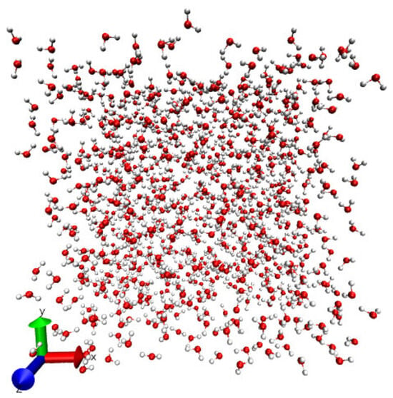
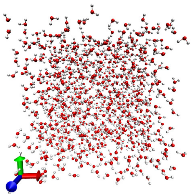
A snapshot of the equilibrium state for a pure water system at 300 K after 20 ns, obtained using the Visual Molecular Dynamics (VMD) program [22] is given as an example in Figure 1.

Figure 1. Snapshot of the equilibrium configuration for a pure water system after 20 ns.

The radial distribution function (RDF),

$$\begin{array}{c}\hfill G\left(r\right)={\displaystyle \frac{1}{\rho }}{⟨{\displaystyle \frac{N(r,\mathrm{\Delta }r)}{V(r,\mathrm{\Delta }r)}}⟩}_i,\end{array}$$

(2)

is a measure of the number of atoms located within a spherical shell of radius $\mathbf{r}$ at a given distance from a reference atom. $\rho$ denotes the number density, $N(r,\mathrm{\Delta }r)$ represents the number of molecules within a spherical shell located between distances $r-\mathrm{\Delta }r/2r$ and $r+\mathrm{\Delta }r/2r$ from the reference molecule, $V(r,\mathrm{\Delta }r)$ is the volume of the shell, and ${⟨(\dots )⟩}_i$ denotes the statistical average.

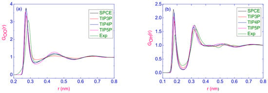
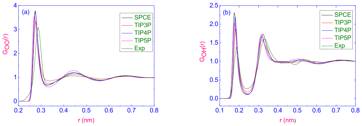
In this study, the RDFs calculated between $\mathrm{O}-\mathrm{O}$, $\mathrm{O}-\mathrm{H}$, and $\mathrm{H}-\mathrm{H}$ atom pairs for pure water systems modeled using the SPCE, TIP3P, TIP4P, and TIP5P water models are presented in Figure 2a,b and Figure 3a, respectively.

Figure 2. The radial distribution functions between pairs of atoms ($\mathrm{O}-\mathrm{O}$ (a) and $\mathrm{O}-\mathrm{H}$ (b)) for pure water systems depending on the radius of r, modeled using the water models SPCE, TIP3P, TIP4P and TIP5P. The experimental data are borrowed from Ref. [23].

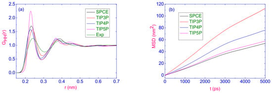
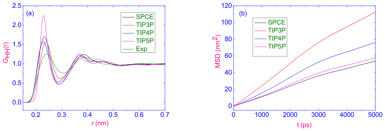
Figure 3. The RDFs between pairs of atoms ($\mathrm{H}-\mathrm{H}$ (a)) and the mean square displacement as a function of time (b) for pure water systems modeled using the SPCE, TIP3P, TIP4P, and TIP5P water models. The experimental data are borrowed from reference [23].

The first peak in the $G\left(r\right)$ functions corresponds to the first coordination shell of the nearest neighbors. The average maxima of the first nearest neighbor peaks in functions $G_{O-O}\left(r\right)$ (see Figure 2a), $G_{O-H}\left(r\right)$ (see Figure 2b) and $G_{H-H}\left(r\right)$ (see Figure 3a), which give the average H-bond lengths of $r_1(O-O)\sim 0.28$ nm, $r_1(H-O)\sim 0.18$ nm, and $r_1(H-H)\sim 0.24$ nm, respectively. The distribution of $\mathrm{O}-\mathrm{O}$ pairs for water molecules in the bulk reveals three layers with a higher probability of the presence of ${\mathrm{H}}_2\mathrm{O}$ molecules. The highest peaks of the RDF $G_{O-O}\left(r\right)$ for oxygen atoms occur around $0.28$ nm, indicating strong binding of the $H_{2}O$ to the $OH$ group. With further increasing of distance r, the height of these peaks drops and at longer range, structure (second and third peaks) starts to disappear, which shows that the ${\mathrm{H}}_2\mathrm{O}$ molecules move away from the $\mathrm{OH}$ groups. It should be noted that the X-ray scattering data for the first maximum of $G_{O-O}$ places it around $0.28$ nm [23].

The mean square displacement (MSD) describes how far the particles are from their original position after a certain time difference, and is defined as

$$\begin{array}{c}\hfill {⟨\mathrm{\Delta }{r}^2\left(t\right)⟩}_i={\displaystyle \frac{1}{N}}⟨{\displaystyle \sum _i^N}{\left({\mathbf{r}}_i(t+t_0)-{\mathbf{r}}_i\left(t_0\right)\right)}^2{⟩}_i,\end{array}$$

(3)

where $t_0$ is the reference time. The calculated values of MSD ${⟨\mathrm{\Delta }{r}^2\left(t\right)⟩}_i$ as a function of time for pure water systems modeled using the SPCE, TIP3P, TIP4P, and TIP5P water models are shown in Figure 3b. Having obtained the MSD, one can determine the diffusion coefficient $D_w$ of the water molecules according to the Einstein relation:

$$\begin{array}{c}\hfill D_w={\displaystyle \frac{1}{6t}}{⟨\mathrm{\Delta }{r}^2\left(t\right)⟩}_i.\end{array}$$

(4)

To calculate the bulk shear viscosity of a system with pure water, we can use the relation

$$\begin{array}{c}\hfill {\eta }_w\left(t\right)={\displaystyle \frac{V}{k_{B}T}}{⟨P_{yx}\left(t\right)P_{yx}\left(0\right)⟩}_i,\end{array}$$

(5)

where

$$\begin{array}{c}\hfill P_{yx}\left(t\right)={\displaystyle \frac{1}{V}}⟨{\displaystyle \sum _{i=1}^N}mv{\left(t\right)}_{ix}v{\left(t\right)}_{iy}+{\displaystyle \sum _{i=1}^{N-1}}{\displaystyle \sum _{j=i+1}^N}{U}_{ij,x}r{\left(t\right)}_{ij,y}{⟩}_i\end{array}$$

(6)

is the shear stress tensor component. Here the sum is over all water molecules in the box of time t, m is the mass of a water molecule, V is the volume of the box, $U_{ij,x}$ is the x-component of the total force on particle i due to particle j, $r_{ij,y}$ is the y-component of the vector ${\mathrm{r}}_i-{\mathrm{r}}_j$, and ${⟨\dots ⟩}_i$ denotes the ensemble average in thermal equilibrium. The kinetic contribution to the pressure is given by the first term in Equation (6), and the virial contribution by the second.

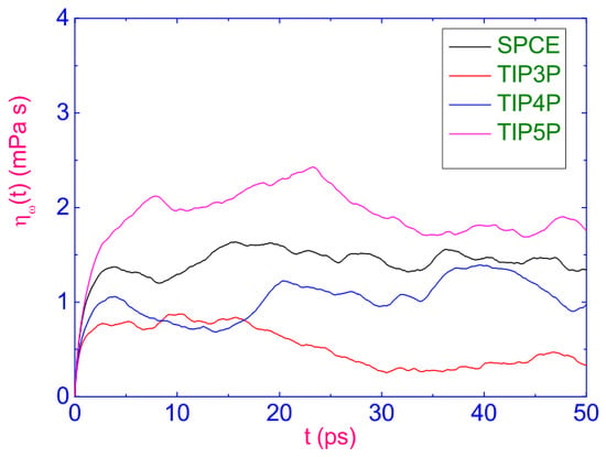
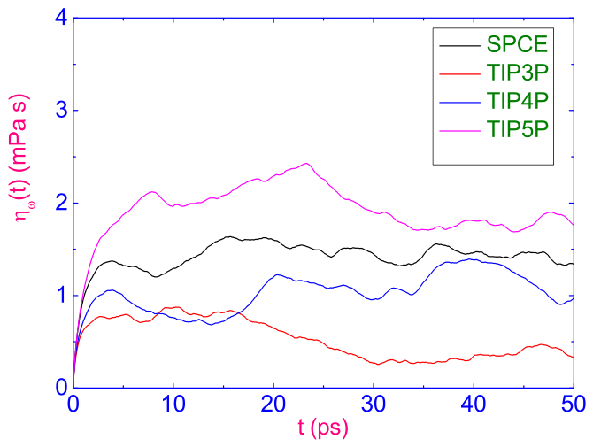
The calculated values of shear viscosity ${\eta }_w\left(t\right)$ as a function of time for pure water systems modeled using the SPCE, TIP3P, TIP4P, and TIP5P water models are shown in Figure 4.

Figure 4. The shear viscosity ${\eta }_w\left(t\right)$ as a function of time for pure water systems modeled using the SPCE, TIP3P, TIP4P, and TIP5P water models.

It should be noted that the calculated values of bulk shear viscosity ${\eta }_w$ were formally obtained with an infinite time limit. However, since the total integrated time correlation function exhibits significant fluctuations over a long period of time, viscosity values are usually determined after reaching the first plateau by considering values within a short correlation time interval of this plateau [24]. In the present study, the viscosity values were obtained by averaging the values on the first plateau of the viscosity–time curves shown in Figure 4. For example, for the TIP3P model, the viscosity was calculated by averaging the values in the time range from 2 to 7.2 ps, which gave a value of $0.76$ m Pa s. Table 2 shows the values of diffusion $D_w$ and shear viscosity ${\eta }_w$ coefficients for pure water systems modeled using the SPCE, TIP3P, TIP4P, and TIP5P water models, respectively, obtained from the MD trajectories for which the simulation was performed.

Table 2. Diffusion $D_w$ and shear viscosity ${\eta }_w$ of water molecules for pure water systems modeled using the SPCE, TIP3P, TIP4P, and TIP5P water models and the experimental data (EXP) [25] at a temperature of 300 K.

$\mathbf{Water}\mathbf{Model}$	${\mathbf{D}}_{\mathbf{w}}\times {10}^9[{\mathbf{m}}^2/\mathbf{s}]$	${\mathit{\eta }}_{\mathbf{w}}\left[\mathbf{mPa}\mathbf{s}\right]$
$\mathrm{SPCE}$	$2.18\pm 0.03$	$1.32\pm 0.03$
$\mathrm{TIP}3\mathrm{P}$	$4.48\pm 0.07$	$0.76\pm 0.02$
$\mathrm{TIP}4\mathrm{P}$	$3.24\pm 0.04$	$1.02\pm 0.03$
$\mathrm{TIP}5\mathrm{P}$	$2.21\pm 0.05$	$2.13\pm 0.13$
$\mathrm{EXP}$	$2.59\pm 0.025$	$0.89\pm 0.01$

Experimental data on $D_w$ and ${\eta }_w$ were obtained using the NMR technique and the technique involving HTO as a tracer [25], respectively. An analysis of both the diffusion and shear viscosity values shows that although the diffusion coefficient predicted by the TIP3P water model differs to a greater extent from the experimental value, its viscosity value is the closest to the experimental result among the models considered. In addition, the radial distribution functions obtained for TIP3P in this study are in better agreement with experimental distributions than those of other water models. Therefore, the TIP3P water model was chosen as the basic model for studying the effect of gold nanoclusters on both structural properties and dynamics of a host water system.

2.2. Simulations of Au/Water Systems

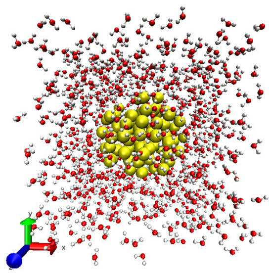
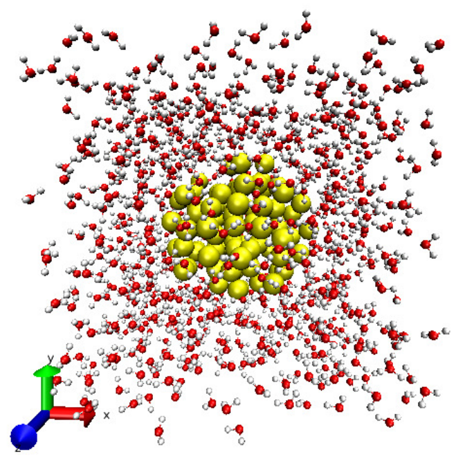
The gold nanoclusters used in the Au/water simulations were generated using the OpenMD program [17]. The nanoclusters were approximately spherical and placed at the center of a cubic simulation box with an edge length of $2.98$ nm, and the remaining volume was filled with a sufficient number of TIP3P water molecules to reproduce the experimental density of this system at room temperature. To study the effect of nanocluster size, we used a Au₁₃ nanocluster with a diameter of 0.6 nm, Au₄₃ with a diameter of 1.0 nm, and Au₈₇ with a diameter of 1.5 nm (see Figure 5).

Figure 5. Snapshot of the equilibrium configuration of the water/Au system with gold nanocluster Au₈₇ with a diameter of 1.5 nm after 200 ns.

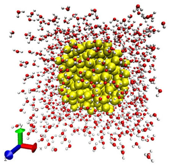
We also modeled Au₂₄₉ (see Figure 6) with a diameter of 2.0 nm.

Figure 6. Snapshot of the equilibrium configuration of the water/Au system with gold nanocluster Au₂₄₉ with a diameter of 2.0 nm after 200 ns.

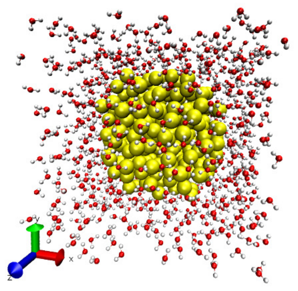
Additionally, we modeled Au₄₅₉ with a diameter of 2.5 nm. Selected details of all simulated Au/water systems are shown in Table 3.

Table 3. The diameter of the Au nanoclusters, the number of Au atoms in a cluster, and the number of water molecules in Au/water systems.

$\mathbf{Water}\mathbf{Model}$	$\mathbf{Au}\mathbf{NC}\mathbf{Diameter}\left(\mathbf{nm}\right)$	$\mathbf{Number}\mathbf{of}\mathbf{Au}\mathbf{Atoms}$	$\mathbf{Number}\mathbf{of}\mathbf{Water}\mathbf{Mol}.$
$\mathrm{TIP}3\mathrm{P}$	$0.6$	13	871
$\mathrm{TIP}3\mathrm{P}$	$1.0$	43	846
$\mathrm{TIP}3\mathrm{P}$	$1.5$	87	818
$\mathrm{TIP}3\mathrm{P}$	$2.0$	249	708
$\mathrm{TIP}3\mathrm{P}$	$2.5$	459	560

Gold atoms were modeled via a 12–6 Lennard–Jones (LJ) potential characterized by ${\mathrm{ffl}}_0=22.145\mathrm{kJ}/\mathrm{mol}$ and ${\mathrm{oe}}_0=0.2629\mathrm{nm}$, adopting the parameterizations proposed in Ref. [26]. These parameters were developed based on the experimental bulk densities and surface tensions of $fcc$ metals and were tested for interfacial systems involving water and organic molecules. The model is also compatible with commonly used molecular force fields such as OPLS-AA [20,21]. However, this classical description does not explicitly account for dynamic electronic polarization or image-charge effects at the metal surface. Comparisons showed that polarization plays a more pronounced role in the interaction of isolated water molecules and charged species with Au surfaces, whereas polarizable and non-polarizable models produced similar water density profiles for liquid water in contact with planar Au surfaces [27]. Therefore, the absence of explicit Au polarization should be considered a limitation of the present model. All simulations of Au/water systems were carried out in the NVT ensemble, and MD simulations of these systems were performed with the GROMACS 5.0.2 program [28,29,30,31]. Regarding the ensemble, we see that pressure is not externally controlled in NVT simulations. However, the same NVT protocol was applied consistently to all systems, with the water content chosen to maintain the water phase close to its experimental bulk density at 300 K. Thus, our goal is not to reproduce the transport properties at a given pressure, but to compare the changes in the structure, diffusion, and viscosity of water depending on the nanocluster size under otherwise comparable modeling conditions.

The system temperature was kept constant at 300 K using a v-rescale thermostat with a coupling parameter of $0.01$ ps, while the time step was assumed to be $0.5$ fs. For non-bonding interactions, the cutoff distance was 1 nm. All systems were run over a simulation time of 200 ns to bring them into equilibrium. Finite-size and periodic-image effects cannot be completely excluded, particularly for the largest Au nanoclusters. Since all systems were investigated using the same box size and boundary conditions, the results are discussed primarily in terms of relative trends with nanocluster size rather than absolute transport coefficients. For the analysis, additional simulation was performed during the simulation time of 5 ns by recording with a frequency of $1.0$ ps. Periodic boundary conditions in three dimensions were used in the simulations. For electrostatic interactions, the Particle Mesh Ewald (PME) approach [32] was used. In addition, to obtain reliable bulk shear viscosity values for all systems, shorter simulations of 250 ps were conducted with a finer data sampling interval of $0.0025$ ps.

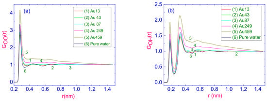
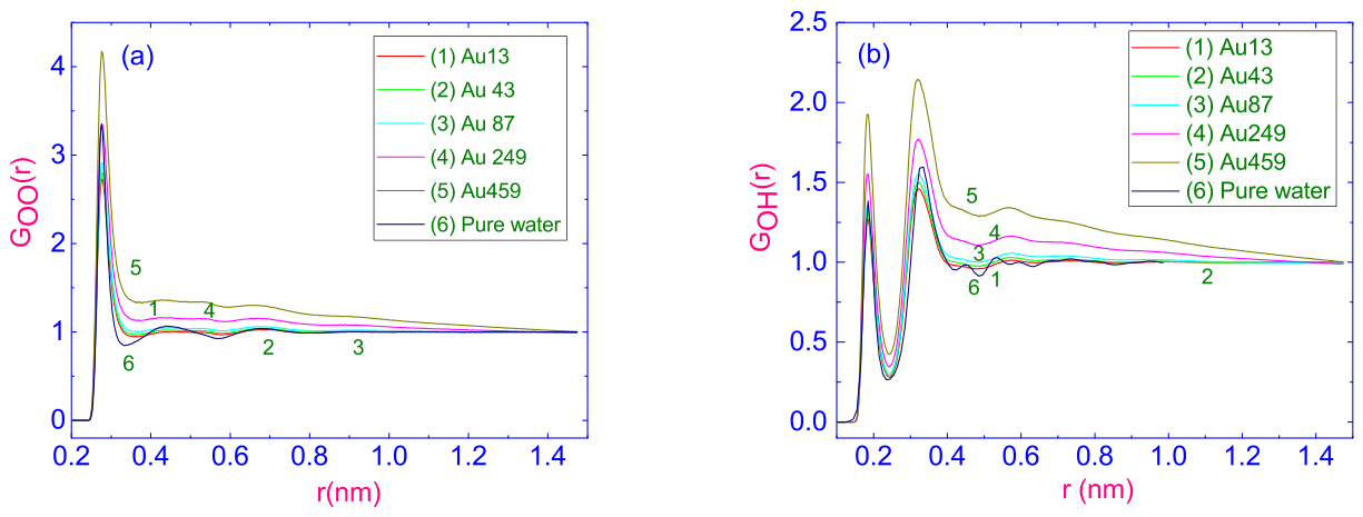
Computer simulations were completed using the computer clusters in the TÜBİTAK TRUBA infrastructure. Snapshots of the equilibrium state obtained using the Visual Molecular Dynamics (VMD) program [22] are given as examples in Figure 5 and Figure 6. The RDFs $\mathrm{G}\left(\mathrm{r}\right)$ between $\mathrm{O}-\mathrm{O}$, $\mathrm{O}-\mathrm{H}$ and $\mathrm{H}-\mathrm{H}$ pairs of atoms in the Au nanocluster/water systems depending on the distance between these atoms r are shown in Figure 7a,b and Figure 8a, respectively.

Figure 7. Radial distribution functions $G\left(r\right)$ between pairs of atoms ($\mathrm{O}-\mathrm{O}$ (a) and $\mathrm{O}-\mathrm{H}$ (b)) for water/gold systems depending on the distance between these atoms r. The meanings of the curve labels from 1 to 6 are explained in the text.

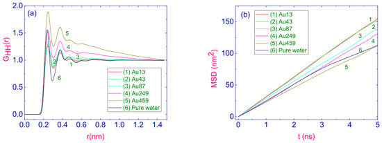
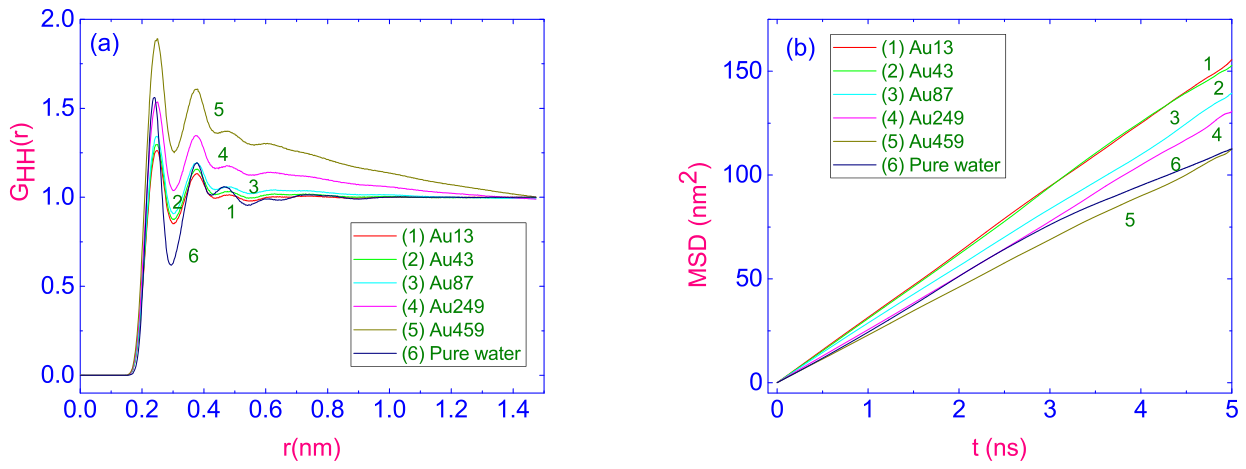
Figure 8. Same as in Figure 7 but for the RDFs $G_{HH}\left(r\right)$ between $\mathrm{H}-\mathrm{H}$ (a) pairs of atoms and the mean square displacement ${⟨\mathrm{\Delta }{r}^2\left(t\right)⟩}_i$ (b) as a function of time t, respectively.

The labels for the curves showing number of equilibrium RDFs $G\left(r\right)$ between $\mathrm{O}-\mathrm{O}$ (see Figure 7a), $\mathrm{O}-\mathrm{H}$ (see Figure 7b) and $\mathrm{H}-\mathrm{H}$ (see Figure 8a) pairs of atoms for nanospherical Au clusters with different diameters and numbers of Au atoms have the following meanings: 1 corresponds to system with a spherical Au₁₃ cluster with a diameter of 0.6 nm, 2 corresponds to one with a spherical Au₄₃ cluster with a diameter of 1.0 nm, 3 corresponds to one with a spherical Au₈₇ cluster with a diameter of 1.5 nm, 4 corresponds to one with a spherical Au₂₄₉ cluster with a diameter of 2.0 nm, and 5 corresponds to one with a spherical Au₄₅₉ cluster with a diameter of 2.5 nm. In turn, 6 corresponds to the pure water system at 300 K, obtained using the water model TIP3P.

First of all, our simulations show the weak effect of the size of Au nanoclusters on the position of the first peak in the $G\left(r\right)$ function corresponding to the first coordination shell of the nearest neighbors. With further a increase in distance r, the height of the second and third peaks drops and they disappear, which shows that the H₂O molecules move away from the OH groups.

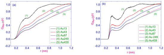
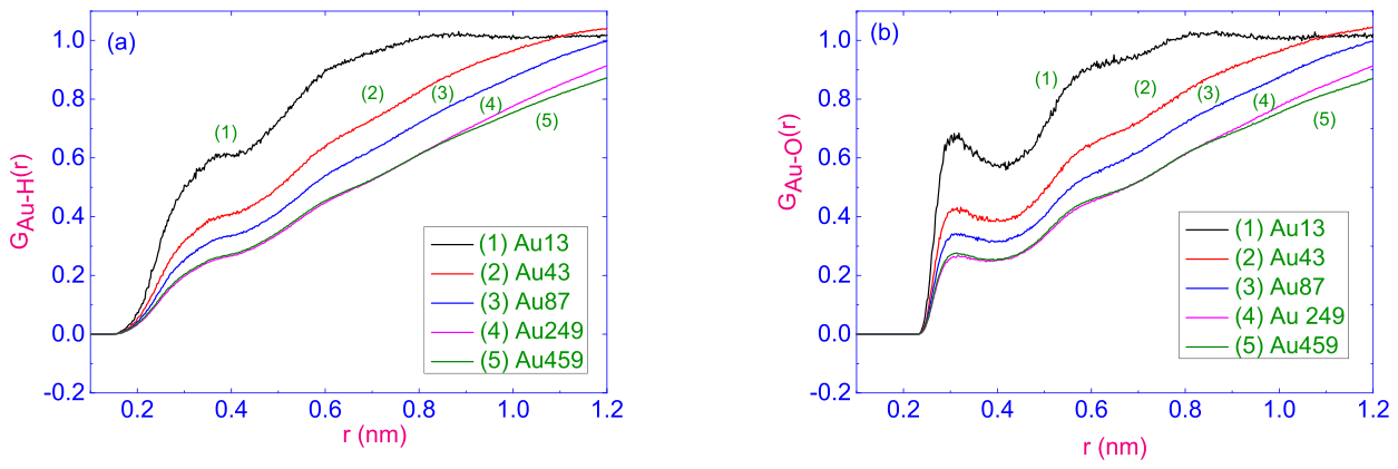
The number of equilibrium RDFs $G_{Au-H\left(O\right)}\left(r\right)$ between Au clusters and $\mathrm{H}$ (see Figure 9a) and $\mathrm{O}$ atoms (see Figure 9b) for spherical Au nanoclusters with different diameters and numbers of Au atoms are shown below with labels as follows: 1 corresponds to a system with a spherical Au₁₃ cluster with a diameter of 0.6 nm, 2 corresponds to one with a spherical Au₄₃ cluster with a diameter of 1.0 nm, 3 corresponds to one with a spherical Au₈₇ cluster with a diameter of 1.5 nm, 4 corresponds to one with a spherical Au₂₄₉ cluster with a diameter of 2.0 nm, and 5 corresponds to one with a spherical Au₄₅₉ cluster with a diameter of 2.5 nm.

Figure 9. (a) Radial distribution functions $G_{Au-H}\left(r\right)$ between Au clusters and H atoms for water/gold systems depending on the distance r. The meanings of the curve labels from 1 to 5 are explained in the text. (b) Same as in (a), but for the RDFs $G_{Au-O}\left(r\right)$ between Au clusters and O atoms.

Our simulations show that the position of the first peak in the $G_{Au-O}\left(r\right)$ function, corresponding to the first coordination shell of the nearest O atoms relative to the Au NC, remains practically unchanged as the size of the nanoclusters varies.

As shown in Figure 8b, the slope of the mean square displacement ${⟨\mathrm{\Delta }{r}^2\left(t\right)⟩}_i$ of the centers of mass of water molecules decreases with increasing nanosphere diameter. By calculating the slopes over different regions of the curves and using the Einstein relation given in Equation (4), the average diffusion coefficients and their standard deviations were obtained and are listed in Table 4.

Table 4. Calculated values of diffusion D and shear viscosity $\eta$ coefficients of water molecules in pure water (TIP3P) and Au/water systems at a temperature of 300 K.

$\mathbf{Diameter}\mathbf{of}\mathbf{Au}\mathbf{NCs}\left(\mathbf{nm}\right)$	$\mathbf{D}\times {10}^9[{\mathbf{m}}^2/\mathbf{s}]$	$\mathit{\eta }\left[\mathbf{mPa}\mathbf{s}\right]$
$\mathrm{Pure}\mathrm{water}$	$4.48\pm 0.07$	$0.76\pm 0.02$
$0.6$	$5.27\pm 0.17$	$4.69\pm 0.37$
$1.0$	$5.22\pm 0.17$	$10.31\pm 0.35$
$1.5$	$4.53\pm 0.15$	$59.35\pm 1.42$
$2.0$	$4.39\pm 0.15$	$\mathrm{N}/\mathrm{A}$
$2.5$	$3.81\pm 0.14$	$\mathrm{N}/\mathrm{A}$

N/A: Shear viscosity could not be reliably determined for the systems containing Au nanoclusters with diameters of 2.0 and 2.5 nm.

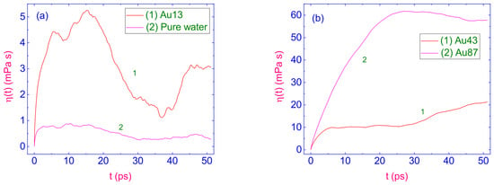
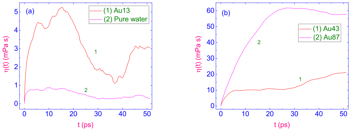
Examination of the results indicates that the diffusion coefficient of water decreases as the size of the gold nanospheres increases. On the one hand, this behavior can be explained by a decrease in the mobility of water molecules due to an increase in the size of Au nanoclusters. On the other hand, the fact that the addition of the smallest Au nanoclusters leads to an increase in the self-diffusion coefficient compared to pure water may be related to the disruption of the tetrahedral hydrogen-bond network. Figure 10a,b show the time evolution of the shear viscosity coefficient of water in W/Au NC and pure water systems.

Figure 10. The calculated shear viscosity $\eta \left(t\right)$ as a function of time t for (a) pure water (TIP3P) and the Au13/water system, and (b) the Au43/water and Au87/water systems. The meanings of curves 1 and 2 are explained in the text.

Here, in Figure 10a, curve 1 corresponds to a system with a spherical Au₁₃ cluster with a diameter of 0.6 nm, and curve 2 corresponds to a system of pure water at 300 K, obtained using the water model TIP3P. In turn, in Figure 10b, curve 1 corresponds to a system with a spherical Au₄₃ cluster with a diameter of 1.0 nm, and curve 2 corresponds to one with a spherical Au₈₇ cluster with a diameter of 1.5 nm. For the reasons discussed above, the viscosity values were determined by averaging the data in the first plateau region on the viscosity–time curves, and the resulting values together with their standard deviations are shown in Table 4. As the diameter of the Au nanoclusters increases, there is a noticeable increase in the viscosity of water. An increase in the diameter of the Au nanoclusters corresponds to an increase in the surface area of the nanoclusters. Consequently, water molecules interact with a larger friction surface, which leads to a decrease in fluidity. It should be noted that the values of $\eta \left(t\right)$ correspond to estimates for the first plateau, the absolute magnitude of which is determined approximately, while the qualitative ranking (pure water $<A{u}_{13}<A{u}_{43}<A{u}_{87}$) is reliable.

It should also be noted that the increase in the viscosity of water molecules in the water/Au system is due to an increase in the size of the Au nanoclusters. We are dealing with more concentrated systems, in which the diffusion process slows down because it occurs in a limited volume of the simulation box. Because the simulation box volume was kept constant, increasing the nanocluster size also increased the Au volume fraction and decreased the number of water molecules. Consequently, the observed size-dependent changes in diffusion and viscosity should be interpreted as arising from the combined effects of nanocluster size and the corresponding change in the relative contribution of the Au–water interfacial region. For the systems containing the larger nanoclusters, particularly those with diameters of 2.0 and 2.5 nm, the reduced separation between neighboring periodic GNC surfaces may also influence the physical properties of the surrounding water. Thus, the calculated values of the diffusion coefficients for these systems may reflect not only the effect of the increased Au–water interfacial area but also the contribution of neighboring periodic surfaces of the nanoclusters. This possible contribution should be considered when interpreting the results for the largest Au nanoclusters.

The present model provides a simplified classical description of the Au–water interface. In particular, the use of non-polarizable Lennard-Jones parameters with zero partial charges does not explicitly account for electronic polarization, image-charge effects, or size-dependent changes in the electronic structure of very small Au clusters. These limitations are expected to be most significant for sub-nanometer particles such as Au₁₃, for which non-bulk geometries and quantum-size effects may become important. Therefore, the present results should be interpreted mainly in terms of relative trends obtained using the same interaction model across different nanoparticle sizes, rather than as a quantitatively exact description of the Au–water interface. More advanced polarizable force fields or ab initio molecular dynamics would be required for a more rigorous treatment of these effects.

3. Conclusions

A key challenge in studying the structural properties of water containing gold nanoclusters (GNCs) is the relationship between molecular properties and phase organization. Molecular dynamics (MD) simulations offer a numerical approach to the problem of the relationship between micro- and macro-properties in such Au NC/water systems. Our MD simulations were carried out to study the structural properties and dynamics of water molecules in Au/water systems. Analysis of the results of MD simulations show that the water diffusion coefficient decreases with increasing size of the gold nanosphere. This behavior can be explained by a decrease in the mobility of water molecules associated with the growth of the nanosphere. Our calculations also show that as the diameter of the Au nanocluster increases up to 1.5 nm in diameter, the viscosity of the water increases markedly. An increase in the diameter of the Au nanocluster corresponds to an increase in the surface area of the nanocluster. Consequently, water molecules interact with a larger friction surface, which leads to a decrease in fluidity. For the largest nanoclusters, the reduced surface-to-surface distance between neighboring periodic images can enhance the retention of water molecules between them and, thus, affect the calculated transport properties. By expanding the range of calculations for the Green–Kubo integral for two of the most complex systems, such as those containing Au₂₄₉ and Au₄₅₉, to time values exceeding 50 ps, we can lay the foundation for further confirmation of the reliability of our results. Our simulations also show the weak effect of the size of Au nanoclusters on the position of the first peak in the $G\left(r\right)$ function corresponding to the first coordination shell of the nearest neighbors. With a further increase in the distance r, the height of the second and third peaks drops and disappears, which shows that the H₂O molecules move away from the OH groups.

The integration of MD simulations into the study of Au nanoparticles dissolved in aqueous systems presents significant potential, but also a number of challenges. Conducting large-scale MD simulations requires significant computing power, which often requires the use of high-performance processing resources and parallel computing using graphics processors to increase efficiency. Without these resources, simulations are performed in a shorter time and with smaller system sizes, which limits their ability to cover the relevant processes. We believe that this study may shed light on the problem of the structure and dynamics of an aqueous system containing gold nanoparticles.

References

- Jia, Y.; Jiang, Y.; He, Y.; Zhang, W.; Zou, J.; Magar, K.T.; Boucetta, H.; Teng, C.; Jia, W.H. Approved Nanomedicine against Diseases. Pharmaceutics 2023, 15, 774. [Google Scholar] [CrossRef] [Scilit] [PubMed]
- Zheng, K.; Song, R.; Li, R.; Liu, M.; Ba, Y.; Jiang, W.; Fan, K. Nanomaterials for refining tumor microenvironment and enhancing therapy in head and neck squamous cell carcinoma: A review. Oncol. Transl. Med. 2024, 10, 151–161. [Google Scholar] [CrossRef] [Scilit]
- Rubicondo, M.; Ciardelli, G.; Mattu, C.; Tuszynskiet, J.A. Drug Discov. Recent advancements in colchicine derivatives: Exploring synthesis, activities, and nanoformulations for enhanced therapeutic efficacy. Drug Discov. Today 2025, 30, 104312. [Google Scholar] [CrossRef] [Scilit] [PubMed]
- Wang, A.; Santos, A.; Evdokiou, A.; Losic, D. An overview of nanotoxicity and nanomedicine research: Principles, progress and implications for cancer therapy. Chem 2015, B3, 7153–7172. [Google Scholar] [CrossRef] [Scilit] [PubMed]
- Mitchell, M.J.; Billingsley, M.M.; Haley, R.M.; Wechsler, M.E.; Peppas, N.A.; Langer, R. Engineering precision nanoparticles for drug delivery. Nat. Rev. Drug Discov. 2020, 20, 101–124. [Google Scholar] [CrossRef] [Scilit] [PubMed]
- Blanco, E.; Shen, H.; Ferrari, M. Principles of nanoparticle design for overcoming biological barriers to drug delivery. Nat. Biotechnol. 2015, 33, 941–951. [Google Scholar] [CrossRef] [Scilit] [PubMed]
- Bhardwaj, H.; Jangde, R.K. Current updated review on preparation of polymeric nanoparticles for drug delivery and biomedical applications. Next Nanotechnol. 2023, 2, 100013. [Google Scholar] [CrossRef] [Scilit]
- Dykman, L.; Khlebtsov, B.; Khlebtsov, N. Drug delivery using gold nanoparticles. Adv. Drug Deliv. Rev. 2025, 216, 115481. [Google Scholar] [CrossRef] [Scilit] [PubMed]
- Ghandi, K.; Findlater, A.D.; Mahimwalla, Z.; MacNeil, C.S.; Awoonor-Williams, E.; Zahariev, F.; Gordonet, M.S. Ultra-fast electron capture by electrosterically-stabilized gold nanoparticles. Nanoscale 2015, 7, 11545. [Google Scholar] [CrossRef] [Scilit] [PubMed]
- Farren-Dai, M.; Awoonor-Williams, E.; MacNeil, C.S.; Mahimwalla, Z.; Ghandi, K. A novel gold nanoparticle stabilization and its muon chemistry. Chem. Phys. Lett. 2014, 610, 331–334. [Google Scholar] [CrossRef] [Scilit]
- Shaffer, T.M.; Pratt, E.C.; Grimm, J. Utilizing the power of Cerenkov light with nanotechnology. Nat. Nanotechnol. 2017, 12, 106–117. [Google Scholar] [CrossRef] [Scilit] [PubMed]
- Haddad, M.; Frickenstein, A.N.; Wilhelm, S. High-throughput single-cell analysis of nanoparticle-cell interactions. TrAC Trends Anal. Chem. 2023, 166, 117172. [Google Scholar] [CrossRef] [Scilit] [PubMed]
- Elliott, A.D. Confocal microscopy: Principles and modern practices. Curr. Protoc. Cytom. 2020, 92, e68. [Google Scholar] [CrossRef] [Scilit] [PubMed]
- Düven, H.E.; Capar, M.I.; Zakharov, A.V. Structural properties of cyanobiphenyl nematics doped with gold nanoparticles: The result of MD simulations. Phys. Lett. 2026, A576, 131388. [Google Scholar]
- Kadaoluwa, S.P.; Meftahi, N.; Elbourne, A.; Weiss, A.C.G.; McConville, C.F.; Padua, A.; Winkler, D.A.; Gomes, M.C.; Greaves, T.L.; Le, T.C.; et al. Systematic Comparison of the Structural and Dynamic Properties of Commonly Used Water Models for Molecular Dynamics Simulations. J. Chem. Inf. Model. 2021, 61, 4521–4536. [Google Scholar] [CrossRef] [Scilit] [PubMed]
- Abascal, J.L.F.; Vega, C. A general purpose model for the condensed phases of water: TIP4P/2005. J. Chem. Phys. 2005, 123, 234505. [Google Scholar] [CrossRef] [Scilit] [PubMed]
- Bhattarai, K.; Majer, T.; Haussmann, M.; Schollmeyer, D.; Kramer, M.; Oni, F.E.; Hofte, M.; Voget, R.; Gutschow, M.; Ruetalo, N.; et al. Department of Chemistry and Biochemistry University of Notre Dame. Notre Dame Ind. 2019, 88, 46556. [Google Scholar]
- Kell, G.S. Density, thermal expansivity, and compressibility of liquid water from 0 to 150 °C: Correlations and tables for atmospheric pressure and saturation reviewed and expressed on 1968 temperature scale. J. Chem. Eng. Data 1975, 20, 97–105. [Google Scholar] [CrossRef] [Scilit]
- Hess, B.; Kutzner, C.; van der Spoel, D.; Lindahl, E. GROMACS 4: Algorithms for Highly Efficient, Load-Balanced, and Scalable Molecular Simulation. J. Chem. Theor. Comput. 2008, 4, 435–447. [Google Scholar] [CrossRef] [Scilit] [PubMed]
- Kaminski, G.A.; Friesner, R.A.; Tirado-Rives, J.; Jorgensenet, W.L. Evaluation and Reparametrization of the OPLS-AA Force Field for Proteins via Comparison with Accurate Quantum Chemical Calculations on Peptides. J. Phys. Chem. 2001, B105, 6474–6487. [Google Scholar] [CrossRef] [Scilit]
- Jorgensen, W.L.; Maxwell, D.S.; Tirado-Rives, J. Development and Testing of the OPLS All-Atom Force Field on Conformational Energetics and Properties of Organic Liquids. J. Am. Chem. Soc. 1996, 118, 11225–11236. [Google Scholar] [CrossRef] [Scilit]
- Humphrey, W.; Dalke, A.; Schulten, K. VMD: Visual molecular dynamics. J. Mol. Graph. 1996, 14, 33–38. [Google Scholar] [CrossRef] [Scilit] [PubMed]
- Soper, A.K.; Phillips, M.G. A new determination of the structure of water at 25 °C. Chem. Phys. 1986, 107, 47–60. [Google Scholar] [CrossRef] [Scilit]
- Hess, B. Determining the shear viscosity of model liquids from molecular dynamics simulations. J. Chem. Phys. 2002, 116, 209–217. [Google Scholar] [CrossRef] [Scilit]
- Lide, D.R. CRC Handbook of Chemistry and Physics. In CRC Handbook, 84th ed.; CRC Press: Boca Raton, FL, USA, 2003. [Google Scholar]
- Heinz, H.; Vaia, R.A.; Farmer, B.L.; Naik, R.R. Accurate Simulation of Surfaces and Interfaces of Face-Centered Cubic Metals Using 12-6 and 9-6 Lennard-Jones Potentials. J. Phys. Chem. 2008, C112, 17281–17290. [Google Scholar] [CrossRef] [Scilit]
- Geada, I.L.; Ramezani-Dakhel, H.; Jamil, T.; Sulpizi, M.; Heinz, H. Insight into Induced Charges at Metal Surfaces and Biointerfaces Using a Polarizable Lennard–Jones Potential. Nat. Commun. 2018, 9, 716. [Google Scholar] [CrossRef] [Scilit] [PubMed]
- Cetin, A.; Capar, M.I.; Zakharov, A.V. Miscibility and diffusivity of water in organic acids: Molecular Dynamics simulations. J. Mol. Liq. 2019, 294, 111630. [Google Scholar] [CrossRef] [Scilit]
- Martínez, J.M.; Martínez, L. Packing optimization for automated generation of complex system’s initial configurations for molecular dynamics and docking. J. Comput. Chem. 2003, 24, 819–825. [Google Scholar] [CrossRef] [Scilit] [PubMed]
- Martínez, L.; Andrade, R.; Birgin, E.G.; Martínez, J.M. PACKMOL: A package for building initial configurations for molecular dynamics simulations. J. Comput. Chem. 2009, 30, 2157–2164. [Google Scholar] [CrossRef] [Scilit] [PubMed]
- Breneman, C.M.; Wiberg, K.B. Determining atom-centered monopoles from molecular electrostatic potentials. The need for high sampling density in formamide conformational analysis. J. Comput. Chem. 1990, 11, 361–373. [Google Scholar] [CrossRef] [Scilit]
- Darden, T.; York, D.; Pedersen, L. Particle mesh Ewald: An N log(N) method for Ewald sums in large systems. J. Chem. Phys. 1993, 98, 10089–10092. [Google Scholar] [CrossRef] [Scilit]
Disclaimer/Publisher’s Note: The statements, opinions and data contained in all publications are solely those of the individual author(s) and contributor(s) and not of MDPI and/or the editor(s). MDPI and/or the editor(s) disclaim responsibility for any injury to people or property resulting from any ideas, methods, instructions or products referred to in the content. |
© 2026 by the authors. Licensee MDPI, Basel, Switzerland. This article is an open access article distributed under the terms and conditions of the Creative Commons Attribution (CC BY) license.