


Abstract
The first approximation () of a three-dimensional micropolar elastic prismatic body in moments of displacement and rotation, obtained via Legendre polynomial expansion, is applied to two related problems: field reconstruction and damage identification. In the first problem, two- and three-dimensional field distributions are reconstructed for a simply supported square prismatic body under three loading configurations, with first-order moment loading as the primary case. Two distinct resonances are identified within the framework. At the material cutoff , micro-rotation amplitudes are amplified while translational amplitudes are suppressed (displacement locking). At the geometric cutoff , the bending mode is resonantly excited while micro-rotation remains near its quasi-static level. In the second problem, a scalar damage model is introduced. The material cutoff follows , confirmed numerically for all four decoupled subsystems and different prismatic body thicknesses. Geometric branches remain insensitive to damage, producing a spectral separation that may serve as a damage indicator. A critical thickness is identified where , leading to role reversal between material and geometric branches. Numerical results are presented for the polyurethane foam of Lakes.
1. Introduction
Classical elasticity describes the mechanical response of a continuous body through six stress components and three displacement degrees of freedom, with no account of the rotational motion of material points. This description is adequate for homogeneous materials at length scales large compared to the microstructure, but becomes insufficient when the characteristic size of the loading or deformation is comparable to the characteristic length of the microstructure—as occurs in foams [1], granular media [2,3], bone [4], and structured composites [5].
Micropolar (Cosserat) elasticity extends the classical theory by introducing independent micro-rotation degrees of freedom at each material point, together with couple stresses conjugate to the curvature of the micro-rotation field. The theoretical foundations were established by [6], systematically developed by [7,8], and further elaborated within the couple-stress framework [9,10]. The theory introduces four additional elastic moduli (, , , , and coupling numbers derived therefrom) and a micro-inertia density J, whose identification from wave experiments was addressed by [11,12] and subsequently by a number of other authors [13,14,15]. Experimental confirmation of micropolar effects was reported by Lakes and collaborators in compact bone [4] and polyurethane foam [1,16], the latter providing the material constants used in the present numerical study. The dynamic behaviour of polymer and rubber-like materials with internal damping was studied in [17], motivating the extension of micropolar models to viscoelastic media, which is left to future work in the present paper.
A distinctive feature of micropolar wave propagation is the existence of cutoff frequencies below which certain wave modes cannot propagate. The lowest such frequency, , is a pure material constant determined by the coupling coefficient and the micro-inertia J; it is independent of the domain geometry and the wavelength. This frequency has been identified in the dispersion relations of bulk micropolar media [7,11,12,18,19]. Its systematic characterisation in bounded structural elements—in particular, the simultaneous presence of material and geometric cutoffs and their differential response to microstructural damage—has not, to the best of the author’s knowledge, been addressed in the prior literature.
Thin micropolar bodies have been studied within various two-dimensional plate and shell theories, including direct Cosserat-surface approaches and thickness-reduction methods. The Legendre polynomial expansion method was developed for micropolar prismatic bodies by Nikabadze and Ulukhanyan, providing a systematic framework for deriving a sequence of self-contained two-dimensional theories of arbitrary approximation (N). The classical elastic case can be recovered as a limiting form of the present micropolar formulation. In the classical limit , , the micro-rotational degrees of freedom decouple, the couple-stress tensor vanishes, and the governing equations reduce to those of classical Cauchy elasticity with a symmetric stress tensor.
Subsequently, the method was extended to micropolar prismatic bodies in a series of works [20,21,22,23], with the first approximations () receiving detailed analysis in [2,24]. A key structural property of the system is the decomposition of the twelve governing equations into four independent groups, enabling analytical solution for each group separately and exposing the physical role of each mode. The zero approximation () was analysed in [25].
Related structural theories for micropolar plates have been proposed by Karttunen et al. [5,26] for web-core sandwich panels, and size-effect phenomena in micropolar beams have been studied via the relaxed micromorphic continuum [27,28]. The characteristic bending length in periodic micropolar structures was investigated in [29]. Acoustic transmission in micropolar materials was recently addressed in [13,30].
The identification of material parameters from wave measurements is an inverse problem of considerable practical importance [31]. For micropolar media, the problem is particularly challenging because the additional parameters (, J, ) do not affect classical wave speeds at long wavelengths but manifest only near cutoff frequencies or in dispersive regimes. Wave-based nondestructive evaluation (NDE) has been extensively developed for classical composites and laminates [32,33,34,35], but corresponding methods for micropolar media remain largely unexplored [16,36].
Damage mechanics provides a continuum framework for describing progressive degradation of material properties [37,38,39,40,41]. The reduction of a coupling modulus under damage has been considered in generalised continua in the context of microcrack-induced loss of couple-stress stiffness [36,42], but a systematic study of the resulting cutoff frequency shifts within micropolar prismatic body theories has not, to the best of the author’s knowledge, been reported.
The present paper addresses two complementary problems within the micropolar prismatic body theory. In the first problem, the full two- and three-dimensional field distributions are reconstructed for a simply supported square prismatic body under three load configurations, and the two cutoff resonances ( and ) are characterised in detail. A phenomenon of displacement locking is identified near , with direct implications for the choice of measurement technique (Section 4). In the second problem, a scalar damage model is introduced and the resulting shifts in the cutoff frequencies are characterised across four decoupled groups and a range of prismatic domain thicknesses (Section 5). While the group decomposition and the existence of cutoff frequencies in micropolar media are known from bulk theory, their interplay with thickness-dependent geometry, field reconstruction, and damage-induced spectral shifts within a unified framework has not been addressed previously. The present paper makes the following contributions to micropolar prismatic body theory: (i) identification of the displacement locking effect and its robustness across load configurations; (ii) systematic characterisation of the damage-induced spectral shift across all four decoupled groups, establishing the universal law and its range of validity; and (iii) identification of the critical thickness at which the roles of geometric and material branches are exchanged.
The rest of this paper is organised as follows. Section 2 recalls the governing equations and the group decomposition. Section 2.4 specifies the material parameters. Section 3 formulates the boundary value problem. Section 4 presents the field reconstruction results. Section 5 presents the spectral damage indicator analysis. Conclusions are drawn in Section 6.
2. System of Equations
A system of governing equations for an isotropic micropolar prismatic body is derived by applying the Vekua-type [43] reduction method, wherein the three-dimensional displacement and micro-rotation fields are expanded in Legendre polynomials with respect to the thickness coordinate . As shown in [18,44,45], this reduction transforms the original three-dimensional problem into an infinite two-dimensional system of coupled partial differential equations, where the expansion coefficients—the moments , of order k—serve as the primary unknowns.
To obtain a computationally tractable model, this infinite system must be truncated. In the first approximation , the series is truncated retaining moments of orders and , yielding a closed system of twelve equations.
Remark 1.
The convergence of the Legendre expansion follows from Jackson’s theorem: the truncation error satisfies uniformly in , independently of the physical medium [43]. Consequently, the truncation provides a well-defined first-order approximation with controlled accuracy.
The zeroth-order moments , describe the thickness-averaged displacement and micro-rotation fields, while the first-order moments , capture the thickness-gradient corrections—the leading bending contribution absent in the zero approximation . Each approximation N constitutes a self-contained continuum theory independent of lower-order solutions. The resulting governing system for the twelve primary fields reads:
Here and are the Lamé material parameters; , , , and are the micropolar coupling and curvature parameters; is the mass density; is the micro-inertia density with the internal characteristic length; is the in-plane Laplace operator; and h is the half-thickness of the layer. The generalised load terms are
combining the k-th order moments of the surface stress/couple-stress resultants and body forces/couples.
2.1. Methodological Framework: The Standalone Theory of First Approximation
Within the framework of prismatic body models, each approximation N constitutes an independent and self-contained mathematical framework governed by a closed system of equations in unknowns. The N-th order solution is obtained directly, requiring no prior computation of lower-order solutions.
For , the twelve equations for the zeroth- and first-order moments , , , , , are solved simultaneously as a single closed system. The zeroth- and first-order moments are coupled through the and terms and cannot be separated without altering the theory. In the limit , the coupling terms proportional to and in the stiffness matrices (5)–(8) vanish, and the equations for different Legendre moments decouple. For loading that is uniform across the thickness, all load moments of order vanish by orthogonality of the Legendre polynomials; only the equations for the zeroth-order moments remain forced, while those for higher-order moments are homogeneous and their solutions vanish, yielding : the field is uniform across the thickness and the system reduces exactly to the theory.
2.2. Decomposition into Independent Groups
Introducing the scalar potentials (4), the system (1)–(3) decouples into four independent subsystems of three equations each (Table 1). Each subsystem constitutes a system that yields three distinct dispersion branches, resulting in twelve branches in total—twice as many as in the approximation [18,45].
Table 1.
Independent group decomposition of the approximation.
The stiffness matrices of the four groups are:
- Group I: longitudinal compression and thickness-bending state. Variables: ; ; . Couples the mean in-plane dilatation with the first-order transverse displacement and first-order torsion . Describes longitudinal (P-wave) motion of the mid-surface combined with thickness-bending and micro-rotational response present only in the approximation.
- Group II: transverse bending and shear state. Variables: ; ; . Couples the mean transverse displacement with the first-order dilatation (bending potential) and mean torsion . Governs the classical flexural response of the layer.
- Group III: micro-rotational dilatation and bending state. Variables: ; ; . Couples the mean micro-rotational dilatation with first-order normal micro-rotation and first-order in-plane shear . Governed by micro-inertia J, it has no classical analogue. All three branches start from nonzero cutoff frequencies at , with the material cutoff as the lowest.
- Group IV: normal micro-rotation and in-plane shear state. Variables: ; ; . Couples the mean normal micro-rotation with first-order micro-rotational dilatation and mean in-plane shear . Carries one acoustic branch () and two micro-rotational branches with cutoffs at and . For the Lakes foam, N; this negative value implies that the off-diagonal coupling in softens the micro-rotational response relative to the classical case.where we have introduced
Groups I and II are governed by the translational mass density and describe displacement-dominated motion; Groups III and IV are governed by the micro-inertia density J and describe micro-rotational dynamics with no classical analogue. The four groups are fully decoupled and can be solved independently once the loads are projected onto the corresponding potential variables (Section 3).
2.3. Effective Internal Length and Connection to Gradient Elasticity
Inspection of the four stiffness matrices (5)–(8) reveals that the combination
appears in the diagonal entries of every group, where
The quantity is therefore the effective internal length of the approximation: it combines a purely geometric contribution (vanishing as ) and a material contribution (independent of the domain geometry) into a single structural parameter.
The physical significance of L becomes apparent when the system is reduced to a single sixth-order partial differential equation for the potential by elimination of and from Group I. Retaining the leading (wave-operator) terms and the second-gradient correction , the sixth-order equation takes the form:
where the three length scales entering the correction are the inverse squared length scales of dimension :
with the micropolar coupling number. Note that since . The full equation with all remaining terms is given in Appendix A.
The leading part of (11) admits a Vieta factorisation into three wave operators corresponding to distinct physical modes:
In classical elasticity, only the P- and S-wave factors appear, giving a fourth-order equation. The additional micro-rotational factor raises the order from four to six and is the direct consequence of the independent micro-rotation degrees of freedom of the micropolar medium.
The stiffness coefficient of the in-plane Laplacian in the -equation of Group II equals , directly identifying the analytical factor , which reflects the intrinsic coupling between classical shear and micropolar rotational resistance in the governing constitutive structure, rather than a geometric shear correction factor of the Reissner–Mindlin type. For reference, the empirical constants of classical plate theory take the values (Reissner) or (Mindlin) [46,47]; a direct numerical comparison is not meaningful, as the two theories describe structurally distinct media.
The coefficient
in (11) enters the fourth-order term and therefore governs the gradient-type correction in the reduced equation.
Although the individual contributions have different signs, their combination remains strictly negative for all admissible material parameters. To verify this, note that
where and as follows from the admissibility condition [48], so that and hence . At the same time , , and using , , . The coefficient (14) is therefore strictly negative and does not vanish for any admissible parameter set.
Thus, the higher-order term retains the structure of a gradient-elasticity regularization with effective length L, while and act only as corrections to this gradient contribution rather than introducing independent length scales
The correction term proportional to breaks the pure Vieta factorisation, coupling the three wave modes and generating the dispersive (non-linear –k) behaviour of the theory. In the limit , and : the geometric contribution vanishes and the effective length is governed entirely by the micropolar material parameter . In the limit (reduced Cosserat medium), and : only the geometric gradient survives.
The sixth-order Equation (11) exhibits a formal structural analogy with gradient elasticity theories, where is the first-order moment of micro-rotational curl. The static fourth-order term is analogous to the gradient term of Mindlin’s second-gradient theory [10] and to the simplified form of [49]. Three structural differences distinguish the present model from these classical formulations. First, two length scales depend on the domain thickness h: L through Equation (9), and through Equation (12), while the third length scale is purely material and independent of geometry. This thickness dependence is absent in both [10] and [49]. Second, all three scales derived from the set of micropolar moduli and h, enter the coefficients – (see Appendix A); the corrections and enter the coefficients and alongside the primary length L, modifying the gradient response through the micropolar coupling and longitudinal-wave contributions, respectively. Third, the present model contains dynamic gradient terms , , , which are absent in the classical static gradient elasticity formulations.
2.4. Material Parameters
Numerical results are presented for the polyurethane foam studied by [1,50], whose micropolar parameters are listed in Table 2.
Table 2.
Material parameters of polyurethane foam [1,50]. Note: N . The negative value is consistent with the thermodynamic inequalities, which require but impose no sign constraint on [48].
Two characteristic frequencies follow from the material parameters:
the micropolar (material) cutoff frequency, and
the geometric cutoff frequency of Group II, which scales as and is present only in the and higher approximations.
3. Boundary Value Problem for a Simply Supported Micropolar Prismatic Body
3.1. Geometry and Boundary Conditions
We consider a micropolar elastic layer occupying the domain
where a is the side length of the square plate and is the total thickness. The in-plane coordinates parameterise the mid-surface, and is the through-thickness coordinate.
Simply supported boundary conditions are imposed on all four lateral edges. For the zeroth-order moments:
The same conditions are adopted for the first-order moments:
The normal micro-rotation and satisfy the zero-moment (Neumann-type) condition on the lateral faces by construction.
3.2. Trigonometric Basis
The boundary conditions (17) and (18) are satisfied exactly by the following modal expansions for mode :
for . The corresponding scalar potentials take the forms
The wavenumber components and total wavenumber are
Substituting (19)–(21) intothe system (1)–(3) and using , reduces each group to a algebraic system.
Note: capital , , etc. denote modal amplitudes of the corresponding moment functions.
3.3. Projection of Loads onto Groups
The generalised loads and decompose in the same trigonometric basis as the fields. After substitution, the right-hand side of each group’s algebraic system receives contributions only from specific load components. The correspondence is summarised in Table 3.
Table 3.
Correspondence between generalised load components and the group algebraic systems they excite. Setting any coefficient to zero decouples the corresponding group from external loading.
Denoting the load amplitudes as , , , , the four right-hand side vectors are
Setting any coefficient to zero removes the correspondingexcitation; setting all four to unity gives the fully loaded case.
3.4. Algebraic Systems and Solution
We seek time-harmonic solutions of the form
where is the prescribed excitation frequency. Substituting (24) into the governing equations and using the modal expansions (19)–(21) with , reduces each group to a algebraic system
where are the stiffness matrices (5)–(8), solved at fixed for the modal amplitude vector . Table 4 summarises the solution vectors, load vectors, and mass matrices for each group.
Once the potential amplitudes are known, the displacement and micro-rotation amplitudes are recovered via the Helmholtz decomposition. In the particular case of the fundamental mode (, where ), the relations simplify to:
for .
3.5. Three-Dimensional Field Reconstruction
The full three-dimensional displacement and micro-rotation fields follow from the Legendre polynomial expansion truncated at :
where and are the Legendre polynomials of orders zero and one, with .
The reconstruction (27) captures two physically distinct contributions:
- The zeroth-order fields , are uniform across the thickness and correspond to the mean (membrane/in-plane) response;
- The first-order fields , vary linearly with and describe the bending and through-thickness gradient of each field, which is the feature of the approximation absent in the theory.
In particular, under a purely transverse load with all other load components zero, only Group II is excited: (Group I gives zero response), so is uniform across the thickness. However, the bending potential generates a non-zero first-order in-plane displacement
which is absent when the first-order moments are not considered. This linear through-thickness profile of is the signature of the bending response in the theory and constitutes the principal qualitative difference between the two approximations ( and ).
4. Task 1: Two- and Three-Dimensional Field Reconstruction
4.1. Problem Statement
We consider the simply supported square prismatic body of Section 3 with side m and half-thickness m, loaded by transverse and micro-rotational surface tractions. The load amplitudes , , , and defined in (23) serve as control parameters; setting any coefficient to zero isolates the corresponding physical effect.
The goals of this section are as follows:
- To identify and characterise the two physically independent resonance phenomena predicted by the theory: the material cutoff , at which micro-rotational degrees of freedom are selectively amplified while macro-displacements remain suppressed (displacement locking), and the geometric cutoff , at which the bending mode is resonantly excited while micro-rotation remains near its quasi-static level; each resonance constitutes a spectral dead zone for a different sensor type—a characteristic feature of the micropolar model that has no classical counterpart;
- To reconstruct the full two-dimensional field distributions in selected planes , verifying that the boundary conditions and modal symmetry are satisfied; and to demonstrate that at , the micro-rotation field reaches amplitudes three to four orders of magnitude above the quasi-static level while the displacement field is simultaneously frozen—a localised energy trapping phenomenon that cannot be captured by classical elastic models;
- To display the through-thickness profiles of the displacement and micro-rotation components, demonstrating the kinematic features of the theory: the linear variation of each field with and the role of the first-order moments in describing the antisymmetric (bending) and symmetric (membrane) contributions to the through-thickness distribution;
- To examine the dependence of the response on the excitation frequency, in particular near the material cutoff and the geometric cutoff . To quantify the frequency selectivity: the material cutoff is controlled by the microstructural parameters and J and is independent of the plate geometry; the geometric cutoff is sensitive to the thickness h and insensitive to . This spectral independence allows the simultaneous identification of microstructural and structural parameters from wave experiments—the physical basis for the damage fingerprint developed in Section 5.
All results are presented for the fundamental mode with wavenumber , and for the material constants of Table 2.
4.2. Two-Dimensional Fields
All results in this section are computed for first-order moment loading (, ) unless stated otherwise. This configuration isolates the antisymmetric (bending) kinematic response of the theory and provides the clearest demonstration of displacement locking at . Results for zeroth-order and combined loading are collected in Appendix B.
The spatial structure of each field is fixed by the mode and the boundary conditions; the frequency and load configuration affect only the amplitudes. Results for higher modes are qualitatively identical since the cutoff frequencies are mode-independent (Section 5). Under first-order loading, the zeroth-order moments and receive no direct excitation (Groups II and IV have zero right-hand side). As a result the following holds:
- At the midplane : the fields and vanish identically—the midplane is a node for both transverse displacement and normal micro-rotation. The in-plane fields , , , and vanish theoretically at due to the pure anti-symmetry of the first-moment loading. In numerical computation, they evaluate to absolute machine zero (–) and exhibit no resonant behaviour. The two-dimensional contour plots at confirm this: and maps are uniformly zero. For this reason, no midplane figures are shown for first-order loading: they carry no physical information beyond the verification of antisymmetry.
- At the top surface , the reconstruction takes the form implying contributions from both zeroth- and first-order moments. Near the critical frequency , the first-order micro-rotation amplitude increases by three to four orders of magnitude and satisfies , so the surface response is governed predominantly by the first-order term. In this regime, is activated only through coupling under first-order loading, whereas determines the resonant behaviour at the top surface.
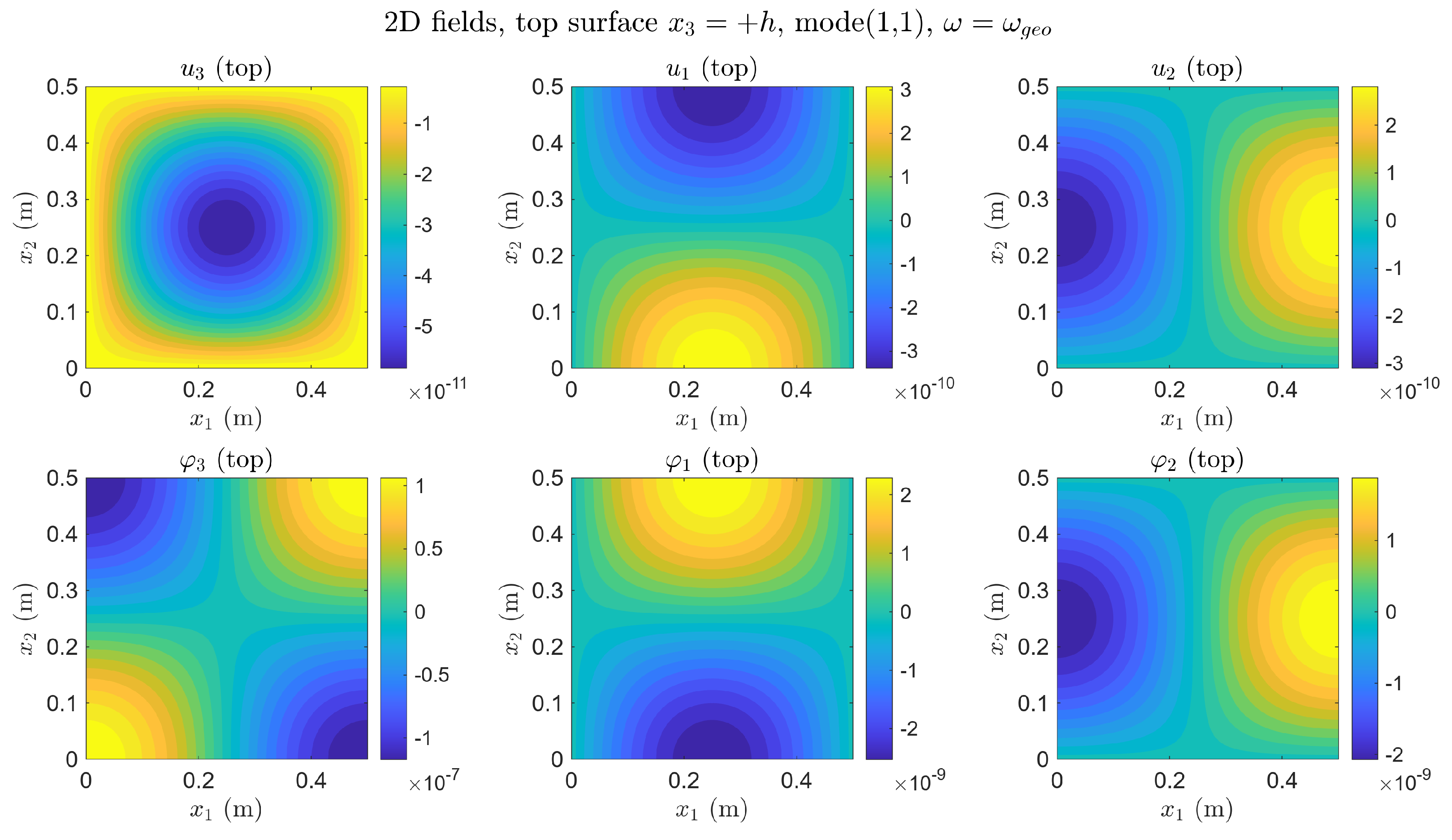
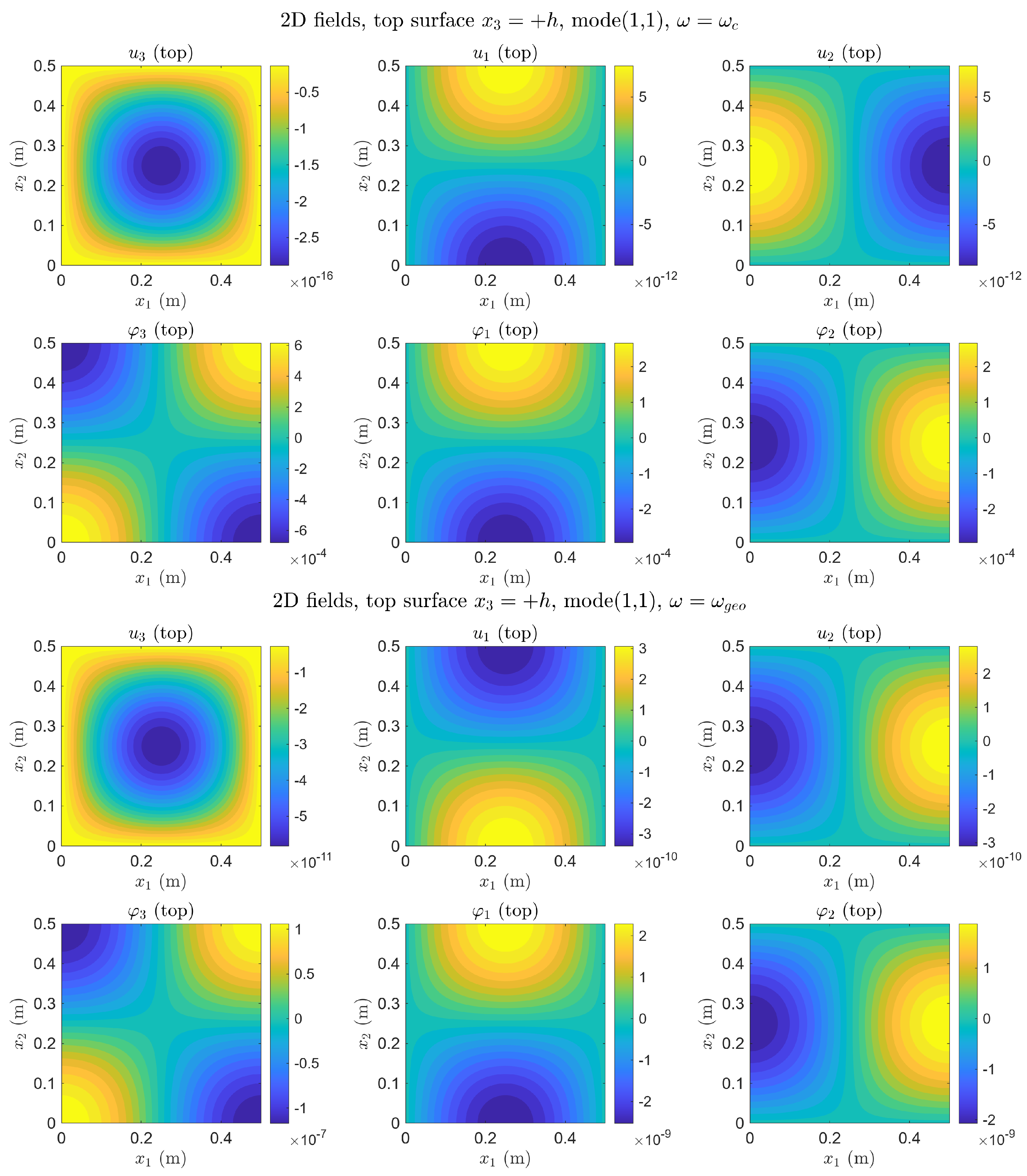
Figure 1 shows the two-dimensional distributions at the top surface at , and Figure 2 at . These two frequencies represent the two physically complementary regimes identified in Section 4.5.
Figure 1.
Top surface , , first-order loading. is thirteen orders of magnitude below (≈ vs. ≈); and are seven orders of magnitude below and (≈ vs. ≈)—displacement locking. Compare with Figure 2.
Figure 2.
Top surface , , first-order loading. Displacements (top row) are amplified at geometric resonance; micro-rotations (bottom row) remain at a quasi-static level . The complementary dead zone: no resonance signal in . Compare with Figure 1.
The two figures together illustrate the complementary nature of the two resonances within the present model: at , the micro-rotation map is active and the displacement map is near-zero; at , the roles are reversed.
4.3. Through-Thickness Profiles
The three-dimensional reconstruction (27) produces a linear profile in for each field component.The profiles of all six field components at are collected in Appendix B (Figure A4). The observation points are
chosen so that the corresponding spatial basis function is non-zero.
The linearity follows directly from the system truncation (27) and holds by construction. The physically significant information is contained in the values and ratios of and , which depend on the frequency and the load configuration.
Effect of the Load Order
Three load configurations are examined. Table 5 summarises the profile character for each configuration; full profiles at all four frequencies are given in Appendix B.
Table 5.
Symmetry of field profiles at for different load configurations. S = symmetric (constant in ); A = antisymmetric (linear, zero at midplane); S + A = superposition (linear, offset from zero).
- Zeroth-order loads only (, ): Groups I and III receive zero right-hand side, so the through-thickness profiles consist of the zeroth-order terms only: , , both independent of , since the first-order solution amplitudes and vanish. The profiles of and are constant across the thickness (symmetric, zeroth-order only): and , independent of . All layers coincide—the plate responds as a membrane without a through-thickness gradient. Crucially, is non-zero at the midplane but does not grow towards the surface: the micro-rotation is uniform across the full thickness, a volume rotation in which every layer of the plate participates equally. The profile of is linear (antisymmetric), generated by the internal coupling in Group II even without direct first-order excitation: with driven by through the term.
- First-order loads only (, ): Groups II and IV receive zero right-hand side, so and . The midplane fields and vanish identically; the two-dimensional contour plots at are uniformly zero, confirming the antisymmetric (bending) character of the first-order excitation. The through-thickness profiles are purely linear, passing through zero at . This is the bending rotation mode: the upper half of the plate () rotates in one direction, the lower half () in the opposite, and the midplane is a rotational node. The spatial in-plane pattern of is the same four-lobe form as in case 1, but the amplitude now changes sign across the thickness. The analogy with classical plate bending is exact: zeroth-order loads excite the membrane (symmetric) mode, first-order loads excite the bending (antisymmetric) mode—but here the field undergoing bending is the micro-rotation , not the transverse displacement . At , while (see Section 4.5.1).
- All loads unity (): The response is the superposition of cases 1 and 2. Profiles are linear but offset from zero at the midplane; the layers separate visibly, demonstrating the combined membrane-bending response. At , this superposition produces a profile in which ∼ (volume component, from case 1) and ∼ (sum of volume and bending components), reflecting a simultaneous resonance of distinct subsystems (Group I and Group IV) at the same material frequency , which manifests as a coupled volume-bending resonant state. Simultaneously, ∼–: displacement locking is complete regardless of whether the micro-rotation profile is symmetric, antisymmetric, or mixed.
4.4. Layer-by-Layer Fields Along the Horizontal Axis
Figure 3 and Figure 4 show the field components , , and along at five thickness levels
at the two resonance frequencies and , with all loads equal to unity. The corresponding plots at and are given in Appendix B.
Figure 3.
Layer-by-layer fields along at (material cutoff), first-order moment loads, mode . (Left): at —amplitude ∼–, nearly frozen despite active loading. (Centre): along at —moderate layer separation, amplitude ∼. (Right): at —amplitude ∼–, three to four orders of magnitude above the quasi-static level. The simultaneous suppression of and amplification of constitutes the displacement locking effect (Section 4.5.1).
Figure 4.
Layer-by-layer fields along at (geometric cutoff), first-order moment loads, mode . (Left): at —amplitude ∼, resonant amplification relative to the quasi-static case. (Centre): at —maximum fan-shaped layer separation among all four frequencies examined, amplitude ∼. (Right): at —amplitude ∼, essentially the same as at : the micro-rotation does not respond to the geometric resonance.
The spatial form of each field along is fixed by the mode and the boundary conditions: ∼, ∼, ∼ (evaluated at the respective values in (29)). What changes with frequency and load is the amplitude of each layer curve and the degree of layer separation.
The fan-shaped separation of the curves is the principal kinematic signature of the theory under bending excitation. Within the framework, the coupling term in Group II generates a non-zero bending potential and, via (26), a non-zero first-order amplitude , producing the linear through-thickness profile (28). The magnitude of this bending effect depends on the excitation frequency and reaches its maximum near .
At (Figure 3, top row): the curves for all five layers nearly coincide at amplitude ∼–—transverse displacement locking occurs: the out-of-plane displacement is suppressed while the in-plane and rotational fields remain finite. The curves show moderate fan-shaped separation at amplitude ∼. The curves are strongly separated: the layer at reaches ∼, the layer at reaches ∼, and the layer at reaches ∼—the bending rotation resonance is superimposed on the volume rotation resonance. The crossing of the curves at the midplane is the signature of the antisymmetric (first-order) contribution; the non-zero midplane value reflects the symmetric (zeroth-order) contribution present under combined loading.
At (Figure 4, bottom row): the situation reverses. The curves separate strongly at amplitude ∼—the bending mode of displacement is resonant. The curves show the maximum fan-shaped separation among all four frequencies examined, amplitude ∼. The curves, by contrast, remain at ∼—essentially the same as in the quasi-static case—and show only mild layer separation. The geometric resonance is transparent to the micro-rotation: a sensor measuring would record no resonance at .
4.5. Frequency Dependence
All results in this subsection are computed for first-order loading throughout, as in Section 4.2.
Figure 3 and Figure 4 show the layer-by-layer distributions at the two physically critical frequencies and ; the quasi-static cases and are presented for completeness in Appendix B.
Two distinct resonance phenomena are observed, each activating a different set of degrees of freedom while leaving the other nearly unaffected.
4.5.1. Material Cutoff: Micro-Rotational Resonance and Displacement Locking
At , the determinant of the Group III system (25) passes through zero, producing a sharp increase in the micro-rotation amplitude . The amplitudes and grow by three to four orders of magnitude compared to the quasi-static case .
A crucial observable at is the displacement locking effect: while the micro-rotation amplitudes reach their resonance peak, the translational amplitudes are simultaneously suppressed. Near , the response is dominated by rotational degrees of freedom, corresponding to an eleven-to-twelve order-of-magnitude separation between rotational and translational amplitudes in the undamped model; the effect of damping is not considered here. This energy transfer from translational to rotational motion is a characteristic feature of the present micropolar model, not present in the corresponding classical elastic formulation.
The amplitude contrast is extreme: at , ∼–, while ∼–—a ratio of eleven to twelve orders of magnitude. A classical displacement sensor would record a negligible response: no detectable motion occurs at the macro-scale. Yet the micropolar microstructure is in full resonance. We refer to this frequency band as a spectral dead zone for classical instrumentation: the material cutoff is effectively undetectable by displacement sensors in the undamped model considered here. (While material damping in polymers such as the Lakes foam will inevitably bound resonance peaks and smooth sharp transitions, the present undamped elastic analysis is essential for isolating the fundamental kinematic coupling mechanisms of the model.)
The locking effect is observed consistently across all three load configurations examined. Under zeroth-order loads only (, ), the entire plate oscillates synchronously (all layers in phase); the micro-rotational resonance occurs simultaneously throughout the full thickness—a volume resonance. The micro-rotation field is non-zero and spatially uniform across the thickness, with the four-lobe in-plane pattern present at every layer simultaneously. Under first-order loads only (, ), the resonance has an antisymmetric character: the upper and lower halves of the plate rotate in opposite directions, while the midplane remains a node—a bending resonance of micro-rotation, the rotational analogue of classical plate bending. The spatial pattern is identical (four-lobe ), but the amplitude varies linearly from at through zero at the midplane to at . Under combined loading (all amplitudes unity), the response is a superposition: the micro-rotation profile is linear in but offset from zero at the midplane, with ∼ and ∼—the constant (volume) and gradient (bending) contributions coexist, and the whole volume of the plate participates in the resonance at every depth. In all three cases, the resonance occurs at the same frequency , confirming that it is an intrinsic material property independent of the load configuration.
This selective amplification of micro-rotational degrees of freedom is determined solely by the ratio , independent of the domain geometry.
Remark 2.
The displacement locking effect has a direct consequence for nondestructive evaluation. Near , classical displacement-based sensors record a very weak response while the material exhibits strong micro-rotational activity; conversely, near , rotation-sensitive measurements show limited response to the geometric resonance. These complementary sensitivity limitations suggest that rotation-sensitive measurement techniques may be required for a more complete characterisation of micropolar media (see also Section 5.5). Experimentally, accessing micro-rotational amplitudes in this spectral dead zone requires advanced optical techniques capable of resolving rotation-related fields rather than standard displacement measurements.
4.5.2. Geometric Cutoff: Bending Resonance
At , the Group II system approaches resonance, producing the maximum separation of the layer curves for (centre panel, Figure 4). The displacement reaches ∼—four to five orders of magnitude above the quasi-static level—while ∼ remains essentially unchanged from the quasi-static value. This is the geometric counterpart of displacement locking: at , the bending mode absorbs the load energy, and the micro-rotation does not respond. A rotation-sensitive sensor placed at would record the quasi-static baseline—a dead zone for rotational instrumentation. Unlike , the geometric cutoff scales as and shifts to higher frequencies as the plate is made thinner, providing an independent spectroscopic indicator sensitive to the domain geometry.
4.5.3. Two Independent Spectroscopic Indicators and Their Observational Consequences
The simultaneous presence of two cutoff types—material and geometric —in a single approximation is the key finding of the present analysis. Their independent tunability allows, in principle, the simultaneous identification of microstructural parameters (, J) and structural geometry (h) from wave experiments.
The two cutoff frequencies are spectrally independent in the sense that depends on and J but not on geometric parameters, while depends on h and and is only weakly sensitive to . As shown analytically and confirmed numericallyin Section 5.1 and Section 5.3, this independence holds across the loading configurations considered. Within the damage model , this leads to a shift of proportional to , while remains nearly unchanged, providing a potential spectroscopic indicator of damage.
The material cutoff scales as since : reducing the internal characteristic length shifts the resonance to higher frequencies. Figure 5 (left) shows the normalised FRF versus for three values of :the curves for different values are visually indistinguishable in the normalised variable; the scatter between them is below the line width of the plot. Figure 5 (right) shows the same data on the absolute frequency axis: the resonance peaks are located at , , and kHz, shifted in exact proportion to . This tunability provides a direct engineering principle for sensor design: by controlling the internal microstructure (grain size, cell size in a foam, fibre spacing in a composite) one can position the micropolar resonance at any target ultrasonic frequency, making accessible to standard transducer technology—provided that rotation-sensitive detectors are employed.
Figure 5.
(Left): Normalised FRF vs. at the top surface for three values of . All curves collapse onto a single master curve, demonstrating scale-invariance of the micro-rotational resonance. The scatter between curves for different is below the line width of the plot. Three values of are shown to confirm collapse; the curves are computationally distinct but visually indistinguishable at this scale. (Right): Absolute FRF vs. frequency (kHz) for three values of . Resonance peaks at , , and kHz shift in exact proportion to . Dashed vertical lines mark the analytical values .
Furthermore, microstructural degradation modelled by increases the effective micropolar length as , which is equivalent to an effective increase in . Therefore, damage shifts the resonance peak to lower frequencies—a measurable shift that constitutes the spectroscopic damage fingerprint analysed in Section 5. Here, denotes the undamaged value of the material cutoff, corresponding to .
Remark 3.
The normalised FRF (Figure 5, left) demonstrates the scale-invariance of the micro-rotational resonance: the shape of the response curve depends only on , not on the absolute value of . The absolute FRF (Figure 5, right) demonstrates the tunability: a factor of 10 reduction in (from to m) shifts the resonance by exactly a factor of 10 in frequency (from to kHz), in agreement with . For the Lakes polyurethane foam, kHz falls in the standard ultrasonic diagnostic range. Materials with smaller (dense ceramics, metals) would push to the MHz range; materials with larger (open-cell foams, granular media, trabecular bone) would bring down to tens of kHz—into the acoustic range accessible to conventional audio transducers, although rotation sensitivity remains the essential requirement.
Remark 4.
The cutoff frequencies and are independent of the in-plane dimensions a and b and the mode numbers . The mode wavenumber affects the amplitudes of the group solutions (25) but not the pole structure: the cutoff frequencies are determined by the k-independent diagonal entries of the stiffness matrices . This independence is confirmed numerically across all four groups in Section 5.3. Consequently, within the present approximation, the spectral indicator is independent of plate geometry and excitation mode—a property that may be relevant for practical non-destructive evaluation (NDE) applications.
4.6. Parametric Study: Effect of the Micropolar Coupling Constant
The two cutoff frequencies depend on in fundamentally different ways:
For the Lakes polyurethane foam , so ( for the parameters, Table 2) and the two frequencies are well separated: kHz versus kHz (a ratio of ≈460). In this standard regime, the two resonances are independently observable.
As is reduced, shifts downward while remains nearly unchanged. At the critical value
the material and geometric cutoffs coincide and the two resonances interact. For the Lakes parameters at m, this occurs at , giving kHz.
Figure 6 and Figure 7 compare the frequency response functions and for the standard value and the reduced value , computed for four plate thicknesses and the critical thickness .
Figure 6.
FRF (log–log scale) at the top surface for four plate thicknesses and the critical thickness . (Left) (standard ): the dominant peak occurs at the same material cutoff kHz for all thicknesses, confirming the h-independence of . The geometric cutoffs (coloured dotted lines at – kHz) produce small but finite local responses in , four to five orders of magnitude below the material resonance—the two frequency scales are spectrally separated. The critical thickness mm (magenta) lies below the other curves before because its geometric cutoff coincides with . (Right) (reduced , kHz): the peaks diverge rightward from with increasing h, demonstrating mode veering: the material and geometric resonances interact and the peak frequency becomes h-dependent. This behaviour is analogous to the mode veering phenomenon of classical structural dynamics [51], where two eigenvalue branches avoid crossing and exchange modal character.
Figure 7.
FRF (log–log scale) at the top surface . (Left) (standard ): resonance peaks appear near the geometric cutoffs but shifted to lower frequencies relative to the theoretical markers—the micropolar softening effect (see Section 4.6). Deep anti-resonances (minima spanning several orders of magnitude) appear between adjacent peaks, a feature of the undamped micropolar system. At kHz, a tiny response is visible, but it is 8–10 orders of magnitude below the geometric resonance peaks: the displacement locking is nearly complete. (Right) (reduced ): the critical thickness (magenta) exhibits the earliest and richest peak structure; secondary peaks appear near kHz for several thicknesses, confirming the coupled regime in which micro-rotational and bending responses interact across the full frequency range.
Remark 5.
The parametric study reveals two qualitatively distinct dynamical regimes of the micropolar plate:
- Separated regime (, standard α): the material and geometric resonances are independently observable. Micro-rotational energy remains localised near and does not excite macro-displacements (displacement locking). The geometric resonance peaks in appear by approximately below the theoretical cutoff —a micropolar softening effect arising from the coupling term in Group II, which shifts the effective bending frequency downward relative to the classical value .
- Coupled regime (∼, reduced α): the two resonances interact (mode veering); response peaks appear in both and near and shift with h. The critical thickness at which marks the strongest interaction.
The transition between regimes is controlled by the ratio
For the Lakes parameters , this ratio is : the system is deep in the separated regime. Reducing α by a factor of 1000 gives , bringing the two resonances within an order of magnitude and producing the visible interaction in Figure 6 (right).
5. Task 2: Spectroscopic Damage Fingerprint via Cutoff Frequency Shifts
Microstructural degradation is modelled by a scalar damage variable acting on the micropolar coupling constant :
All other material constants (, , , , , , J) are held fixed. The model describes the reduction in cell-wall coupling in a micropolar foam, the loss of trabecular connectivity in bone, or the degradation of fibre-matrix bonding in a composite, within a single scalar parameter.
The selective action on rather than on , is motivated as follows. The parameter controls the rotational resistance of the microstructural elements and the coupling between translational and rotational degrees of freedom. Mechanisms such as inter-grain debonding, progressive micro-cracking, or loss of cell-wall connectivity may reduce this coupling before significantly affecting the bulk compression or shear moduli , . The model therefore captures an early stage of microstructural degradation in which the rotational degrees of freedom decouple, while the classical elastic response is still largely intact. The range of validity of this assumption is material-dependent and requires experimental verification.
In the limit , the model recovers the reduced Cosserat medium (), in which rotational and translational degrees of freedom decouple [18]. This provides a physically meaningful endpoint for damage evolution. The rate equation is left to a companion study (Kachanov–Rabotnov framework [37,39]); here, we analyse the spectral indicator as a function of D for the Lakes polyurethane foam of Table 2.
The cutoff frequencies are obtained by setting in the algebraic systems (25). The resulting eigenvalue problem is independent of the wavenumber and therefore independent of the prismatic domain planform, mode number, and boundary conditions on the lateral faces. The damage fingerprint established below is universal across any prismatic body geometry.
5.1. Analytical Sensitivity
The four stiffness matrices (5)–(8) at contain only through the entries (diagonal) and (off-diagonal). Substituting (33) and computing the eigenvalues, one finds that every branch that carries at shifts as:
Here, denotes the undamaged reference value. Within the present framework, this law holds exactly for branches that are purely material (eigenvalue ), and is a lower bound for coupled branches (eigenvalue , ): the geometric term partially masks the -sensitivity, so the relative shift is smaller in magnitude than , approaching it from above as .
Branches that do not contain in their eigenvalue expression are exactly insensitive to D: their shift is identically zero, not merely small. For the Lakes parameters, the geometric cutoff shift satisfies for Groups II and III (residual coupling through off-diagonal terms), and is exactly zero for the longitudinal branch of Group I.
5.2. Branch Classification
Each group possesses two or three nonzero cutoff branches at , ordered by frequency: for group s. Their physical character (geometric or material) depends on the relative magnitude of the two competing scales:
and can change with h. The critical thickness
for the Lakes parameters marks the transition between regimes.
We label branches by their eigenvalue index and identify their character from the sensitivity plots. Table 6 summarises the classification for all four groups in both regimes.
Table 6.
Spectral branch classification: G = geometric (insensitive to D); M = material (follows ); C = coupled (between G and M, approaches M as ). Standard regime: . Thin-plate regime: . —denotes the acoustic branch (), excluded from the cutoff analysis.
In contrast, Groups II and III exhibit a clear role reversal at the critical thickness , whereby the branch associated with transitions from the upper to the lower position in the spectrum as h decreases through .
Group IV is qualitatively different, as no geometric branch exists at : both nonzero branches contain and are therefore consistently sensitive to damage, independent of h. This makes Group IV a potentially more reliable spectral indicator across all thickness regimes within the present model.
The physical significance of the role reversal at is as follows. In the standard regime (), the lower cutoff of Groups II and III is geometric and therefore insensitive to microstructural damage, while the upper branch is material and shifts with D. As h decreases through , these roles are exchanged: the lower branch becomes damage-sensitive and the upper branch becomes geometry-dominated. Consequently, the operating frequency relevant for damage detection depends on the thickness regime of the specimen. Group IV, which contains no geometric branch at any h, provides a thickness-independent spectral indicator and is therefore the most robust single-group diagnostic within the present model.
Remark 6.
The spectral separation underlying the damage indicator is confirmed numerically in Figure 8: the material cutoff decreases monotonically with damage, while the geometric cutoff varies by less than over for the Lakes parameters. The insensitivity of to α-type damage follows from the smallness of the ratio ; for materials with larger coupling numbers this separation may be reduced.
Figure 8.
Normalised cutoff frequencies as functions of the damage parameter D for the Lakes foam parameters [1,50]. The material cutoff decreases monotonically with damage, while the geometric cutoff varies by less than over , confirming the spectral separation used as the basis of the damage indicator.
5.3. Standard Regime
Figure 9.
Cutoff frequencies vs. damage D, standard regime (). (Top left) (Group I): geometric branch horizontal (, insensitive to D); coupled branch shows four separate curves converging towards as h grows. (Top right) (Group IV): material branch —all four thickness values coincide exactly (only one curve visible, see sensitivity plot): a direct numerical confirmation of h-independence of . Coupled branch : four separate curves, converging at large h. (Bottom left) (Group II): lower branch horizontal (geometric); upper branch —all curves coincide (h-independent, pure ). (Bottom right) (Group III): horizontal (geometric); —all curves coincide (h-independent); coupled (four separate curves).
Figure 10.
Relative frequency shifts vs. damage D, standard regime ( mm). Black dashed line: analytical law (Equation (34)). (Top left) (Group I): geometric branch —shift identically zero; coupled branch converges to analytical from above as h increases. (Top right) (Group IV): material branch —all four thickness values lie exactly on the analytical curve, confirming h-independence of ; coupled branch converges as . (Bottom left) (Group II): lower branch zero to ; upper branch lies exactly on analytical line. (Bottom right) (Group III): zero to %; on analytical line; coupled, converges as .
Exact h-independence of . The purely material branches (, , ) produce identical sensitivity curves for all four thickness values. This is not approximate: the curves are indistinguishable at plot resolution, confirming the analytical result independently of h.
Exact insensitivity of geometric branches. The relative shift of geometric branches is zero to machine precision () for Groups II and III, and analytically zero for Group I.
Coupled branches as a lower bound. For coupled branches, the sensitivity approaches from above as h increases. At finite h the relative shift is less than : the geometric term partially masks the damage signal. For NDE purposes, a coupled branch therefore underestimates the true damage level when used as a single indicator; a purely material branch gives the exact value.
5.4. Thin-Plate Regime: Role Reversal
Figure 11.
Spectral indicator, thin-plate regime ( mm). Group II (top left): for and mm ( mm) the lower branch starts at –700 kHz and decreases with D (carries ); the upper branch is horizontal (carries ). For mm mm, the standard assignment is restored. Group IV (top right): no role reversal; coincides for all h (pure , h-independent); coupled, four separate curves. Group III (bottom): for and mm, the nominally geometric branch becomes damage-sensitive (starts at kHz); the nominally material branch becomes horizontal; is geometric at all displayed h.
Figure 12.
Sensitivity analysis, thin-plate regime. Black dashed line: (Equation (34)). Group II (top left): lower branch : for mm: falls to (damage-sensitive, near-analytical); for mm: zero (geometric, standard regime). Upper branch : for mm: zero (geometric in thin regime); for and 100 mm: lies exactly on the analytical line (material in standard regime). The role reversal is complete: the branch that is zero in the standard regime becomes the damage indicator in the thin regime, and vice versa. Group IV (top right): : all four values of h lie exactly on the analytical line—h-independence confirmed in the thin regime as well. : mm lies on analytical; small h deviates upward. Group III (bottom): : for mm: follows analytical (); for and 100 mm: zero. : for mm: zero; for mm: analytical. The analytical law is followed by whichever branch carries , regardless of which branch that is in a given thickness regime.
Remark 7.
Role reversal and NDE practice. If the plate thickness is not known relative to , the wrong branch may be monitored. A sensor tracking the lower cutoff of Group II or III would observe:
- No damage signal for (the lower branch is geometric, correctly insensitive to D);
- A strong damage signal for (the lower branch now carries , sensitive to D).
One approach to identifying the regime is to measure both branches simultaneously, verify which is h-dependent (geometric) and which is not (), and track the latter. Group IV requires no such identification: both its branches are damage-sensitive at all h, making it a more reliable single-group indicator. From a practical standpoint, the role reversal need not be an obstacle: measuring the h-dependence of both branches simultaneously identifies the operating regime, providing a self-consistent multi-modal spectroscopic procedure. For the Lakes foam, mm corresponds to approximately four cell diameters—a practically accessible regime for thin foam sheets and microporous membrane filters.
5.5. Damage Fingerprint: Summary and Practical Consequences
Table 7 summarises the spectroscopic separation of effects by showing the sensitivity of each observable to each damage type.
Table 7.
Sensitivity of spectral observables to microstructural damage (D) and geometry (). Note that linear approximation valid for ; the exact law is (34).
The spectral separation established in Section 5.1, Section 5.2, Section 5.3 and Section 5.4 suggests that simultaneous observation of both cutoff types from wave experiments may allow the independent assessment of microstructural state and structural geometry, provided the thickness regime relative to is identified first.
5.5.1. Implications for Experimental Identification
While no experimental validation is performed in the present work, the results indicate that the identified spectral features may provide a basis for NDE of micropolar structured media.
First, the coexistence of geometric and material branches provides a means to distinguish between geometry-controlled and microstructure-controlled responses, for example by analysing the dependence of spectral features on the plate thickness h.
Second, the material cutoff frequency , being independent of h and governed solely by the micropolar parameter , serves as a robust indicator of microstructural state. In contrast, geometric cutoffs remain insensitive to damage.
Under the damage model (33), the evolution of directly reflects the degradation of the internal structure, following . This relation suggests that monitoring the shift of the material cutoff frequency may provide a direct measure of damage.
Finally, the results indicate that rotational degrees of freedom play a key role near , which may require rotation-sensitive measurement techniques for experimental validation.
5.5.2. Potential Applications
The identified damage fingerprint may be relevant for a range of micropolar structured media in which the coupling parameter degrades under loading.
In aerospace structures, such as honeycomb sandwich panels, fatigue or impact-induced degradation of cell-wall interactions may lead to a measurable shift of the material cutoff frequency , providing a frequency-domain indicator of internal damage without requiring direct access to the interior.
In biological materials, trabecular bone exhibits a porous architecture that can be interpreted within a micropolar framework. A reduction in effective coupling due to degradation of the trabecular network may, in principle, be reflected in the evolution of , offering a thickness-independent complement to conventional density-based diagnostics.
In cellular solids and foams, progressive debonding or damage of microstructural elements under cyclic loading may be detectable through the proposed spectral fingerprint, potentially enabling early identification of degradation prior to macroscopic stiffness loss.
More generally, the relation suggests the possibility of tracking microstructural damage in time through frequency measurements, provided that the material branch can be reliably identified. In this context, the distinction between geometric and material cutoffs, as well as the role of rotational degrees of freedom near , should be taken into account.
5.5.3. Limitations
The present analysis is subject to the following model restrictions.
The approximation retains only the zeroth- and first-order Legendre moments; higher approximations () may capture additional through-thickness variation not represented in the present model. In the limit , the system reduces to two independent copies of the structure (as shown in [18,45]), confirming internal consistency, but the range of h for which the approximation remains accurate has not been quantified here.
The damage model assumes that microstructural degradation acts selectively on the coupling constant while leaving the Lamé moduli , and the curvature parameters , , and unchanged. This is motivated by the interpretation of as governing the interaction between translational and rotational degrees of freedom at the microstructural scale, which may be selectively reduced by inter-grain debonding or micro-cracking before the bulk elastic response is affected, while extreme macrostructural damage would inevitably degrade the Lamé constants simultaneously, the strict mathematical isolation of serves to define the theoretical upper bound of purely microstructural sensitivity before macroscopic compliance sets in. Whether this assumption is appropriate for specific materials requires experimental verification. Although the formal range of the damage variable is , full degradation is never realised in practice: experimental data indicate that macroscopic fracture initiates at – for most engineering materials [40]. The spectral law (34) is presented over the full analytical range; however, the physically relevant operating window for nondestructive monitoring is , where the linearisation holds.
Finally, the spectral invariance of with respect to domain geometry follows analytically from the eigenvalue condition and holds within the model independently of boundary conditions or planform shape. Its experimental observability in structures of complex geometry cannot be inferred from the present results alone.
The present analysis assumes an undamped system. In a damped micropolar medium, resonance peaks acquire a finite width proportional to the damping ratio, and the amplitude contrast associated with displacement locking would be reduced accordingly. The extension to damped or viscoelastic micropolar solids is left to future work.
The material cutoff frequency kHz predicted for the Lakes foam has not been experimentally verified; the present results identify the spectral features theoretically, and experimental confirmation remains an open task.
6. Conclusions
The first approximation () of the micropolar prismatic body theory has been applied to two problems: one involving a simply supported plate and another that is independent of the domain, yielding the following results.
6.1. Field Reconstruction
The decomposition into four independent groups enables analytical reconstruction of all field components for each mode . The Legendre reconstruction produces linear through-thickness profiles; the zeroth-order moments describe the membrane fields and the first-order moments describe the bending fields. Three load configurations produce qualitatively distinct kinematic signatures (Table 5): zeroth-order loading excites the symmetric mode and first-order loading excites the antisymmetric (bending) mode.
6.2. Two Cutoff Resonances
Two distinct resonances are identified within the framework, each activating a different set of degrees of freedom. At the material cutoff , the micro-rotation amplitude is selectively amplified while the translational amplitude is simultaneously suppressed (displacement locking); this behaviour is observed across all three load configurations examined. At the geometric cutoff , the bending mode is resonantly excited while the micro-rotation remains at its quasi-static level. The two resonances are complementary dead zones for different sensor types (Remark 2 and Section 4.5.2). The complementary dead-zone structure of the two resonances implies that a single-sensor strategy—displacement-only or rotation-only—is insufficient for complete spectral characterisation of micropolar prismatic bodies.
6.3. Parametric Study
Two dynamical regimes are identified depending on the ratio c/: a separated regime (c ), in which the two resonances are independently observable, and a coupled regime (∼c), in which mode veering occurs and the resonance peaks become thickness-dependent. The transition is controlled by the ratio
For the Lake parameters, this ratio is 461.9, placing the system well within the separated regime.
6.4. Spectral Damage Indicator
Under the scalar damage model , the material cutoff shifts according to the exact law (34) independently of plate geometry, mode number, and load configuration, and consistently across all four groups. Geometric cutoffs are insensitive to -type damage to machine precision for the Lakes parameters. This spectral separation—a shift in with negligible shift in —may, in principle, allow the independent assessment of microstructural and geometric changes from wave measurements; practical realisation requires rotation-sensitive transducers capable of operating in the relevant frequency range, which, for the Lakes foam parameters, is approximately 718 kHz.
6.5. Critical Thickness and Role Reversal
A critical thickness mm is identified at which . For , the lower cutoff of Groups II and III is geometric (insensitive to D) and the upper is material (sensitive). For , these roles are exchanged. Group IV contains no geometric branch at and its branches are material at all h, constituting the most reliable single-group spectral indicator within the present model, as both its branches are damage-sensitive at all h.
6.6. Outlook
Several directions are suggested for companion studies. First, a natural extension of the present framework concerns the second approximation (), in which the governing equations decompose into four independent subsystems of sizes , , , and , preserving the same group structure and physical classification of wave modes. Second, the identification of the micropolar material constants from wave measurements at varying thicknesses, and the incorporation of a damage evolution law to describe progressive microstructural degradation through the time-varying cutoff . Third, the extension of the present undamped analysis to damped or viscoelastic micropolar media, in which resonance peaks acquire finite width and the amplitude contrast associated with displacement locking is reduced.
Funding
This research received no external funding.
Data Availability Statement
No new data were created in this study; all results follow from the analytical model presented in the article.
Acknowledgments
All figures presented in this manuscript were created by the author, and no copyrighted material from external sources has been used.
Conflicts of Interest
The author declares no conflicts of interest.
Appendix A. Sixth-Order Equation for the First-Order Moment Torsion Potential
The first-order torsion satisfies a sixth-order partial differential equation obtained by eliminating and from Group I (5):
where we have introduced the effective internal length L; . The dimensions and physical interpretation of the coefficients – are given in Table A1; the dimensional analysis of the right-hand side F is summarised in Table A2. The occurrence of the effective length L and the correction terms , across the coefficients and the forcing term is detailed in Table A3. The sixth-order Equation (A1) exhibits a formal structural analogy with gradient elasticity theories [10,49]; the correspondence is summarised in Table A4 and discussed in Section 2.3.
Table A1.
Dimensions and physical interpretation of the coefficients –.
Table A2.
Dimensional analysis and components of the right-hand side function F.
Table A3.
Occurrence of the effective length L and correction terms , in the sixth-order Equation (A1). Checkmark indicates explicit appearance; dash indicates absence.
Table A4.
Correspondence between the characteristic lengths , of the present micropolar prismatic body theory and the length scales of gradient elasticity theories. The primary length L combines a geometric contribution and a material contribution ; the corrections and are derived from the full set of micropolar moduli and the domain thickness h via Equations (9)–(12).
Appendix B. Complete Field Distributions for Task 1
Thickness profiles, layer-by-layer fields, and top-surface two-dimensional distributions are collected here for all three load configurations at four frequencies , , , and . Midplane () two-dimensional fields are omitted: under first-order loading, they vanish identically; under zeroth-order and combined loading, they duplicate the top-surface patterns without additional physical content. Top-surface fields are shown only at the two resonance frequencies and , where the contrast between displacement and micro-rotation responses is physically meaningful.
Appendix B.1. Zeroth-OrderLoads Only
Under zeroth-order loading, the profiles of and are constant across the thickness (membrane/volume mode); and vary linearly through internal coupling. At : ∼ uniform across the full thickness (volume rotation resonance), ∼. At : fan-shaped separation is maximum, unchanged (Figure A1, Figure A2 and Figure A3).
Appendix B.2. First-Order Loads Only
Appendix B.3. All Loads Unity
Under combined loading, the response is the superposition of B.1 and B.2: profiles are linear with non-zero midplane value (offset from zero). At : ∼ (volume component from B.1), ∼ (sum of volume and bending components); ∼–. The entire volume participates in the micro-rotational resonance, with surface layers rotating approximately ten times more strongly than the midplane (Figure A7, Figure A8 and Figure A9).
Figure A1.
Thickness profiles, zeroth-order loads only. , : constant (symmetric). , : linear (antisymmetric, from internal coupling). Bottom left—third panel (): ∼ uniform; ∼ (locking). Bottom right—fourth panel (): slope maximum; unchanged.
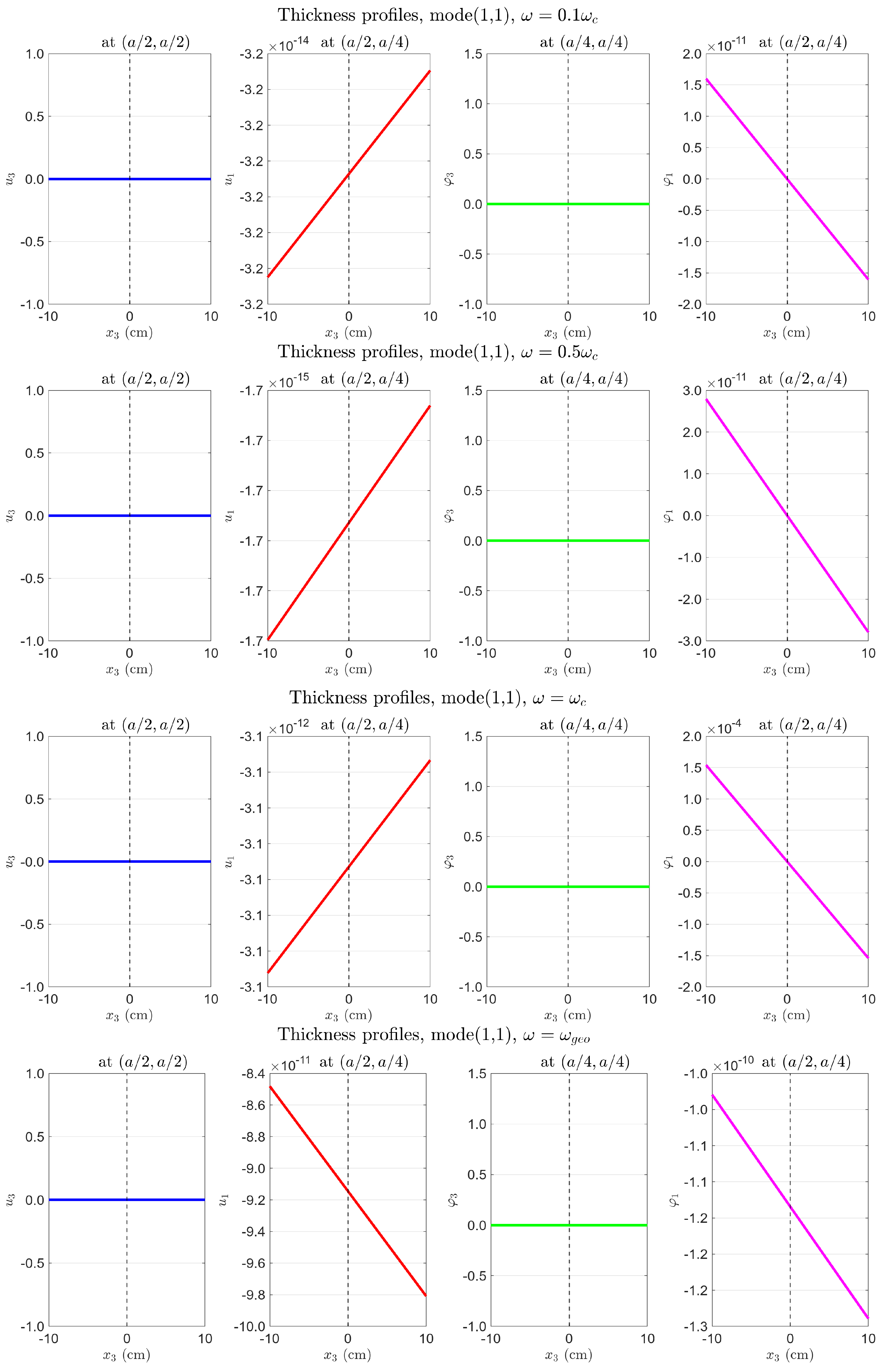
Figure A2.
Layer-by-layer fields along , zeroth-order loads only. : all layer curves coincide (no -gradient, membrane mode). curves cross only weakly (small first-order coupling). See Section 4.5.1 for physical interpretation.
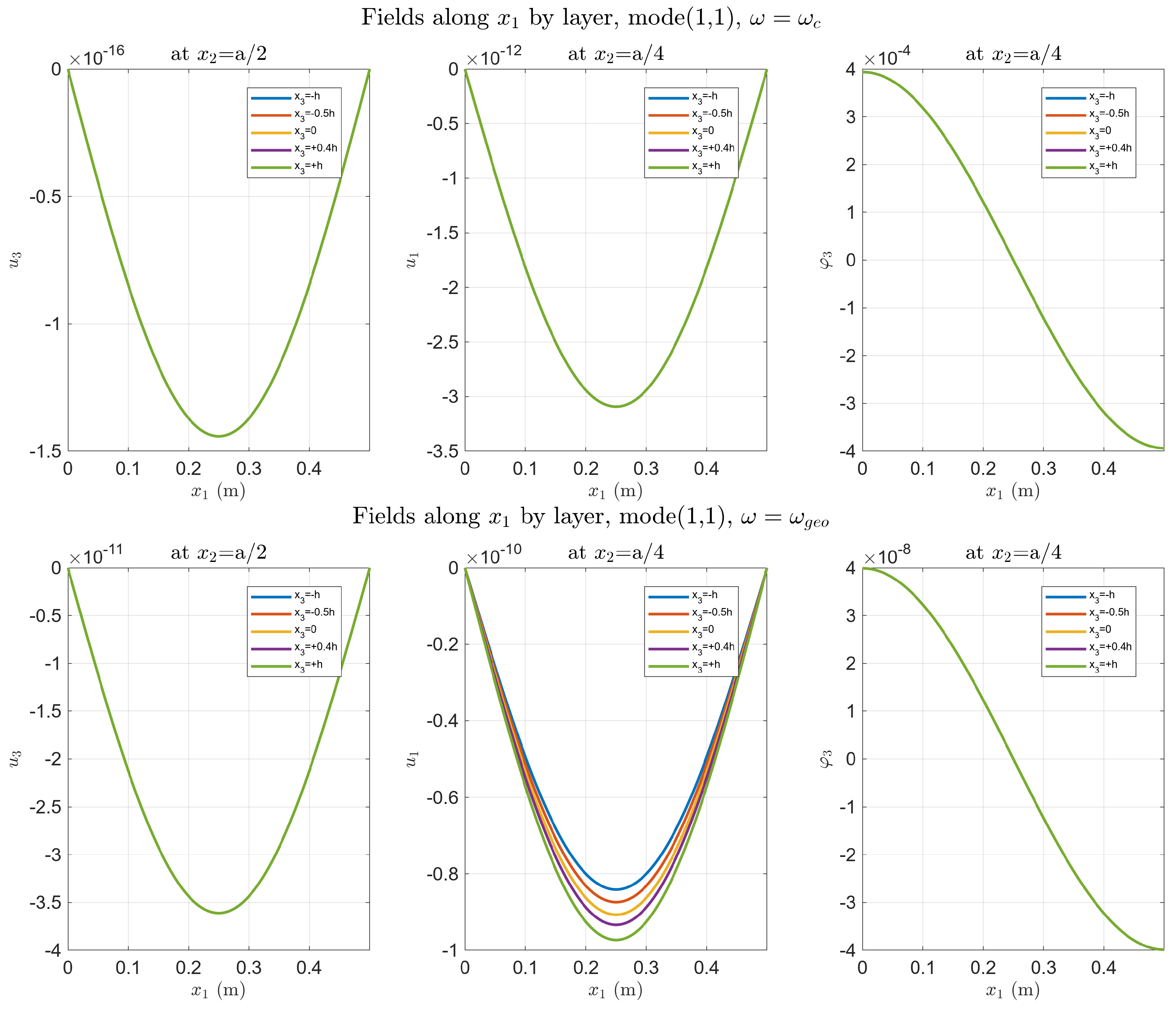
Figure A3.
Top surface , zeroth-order loads only. (Upper) (): (four-lobe, volume resonance); (locking). (Lower) (): amplified; unchanged.
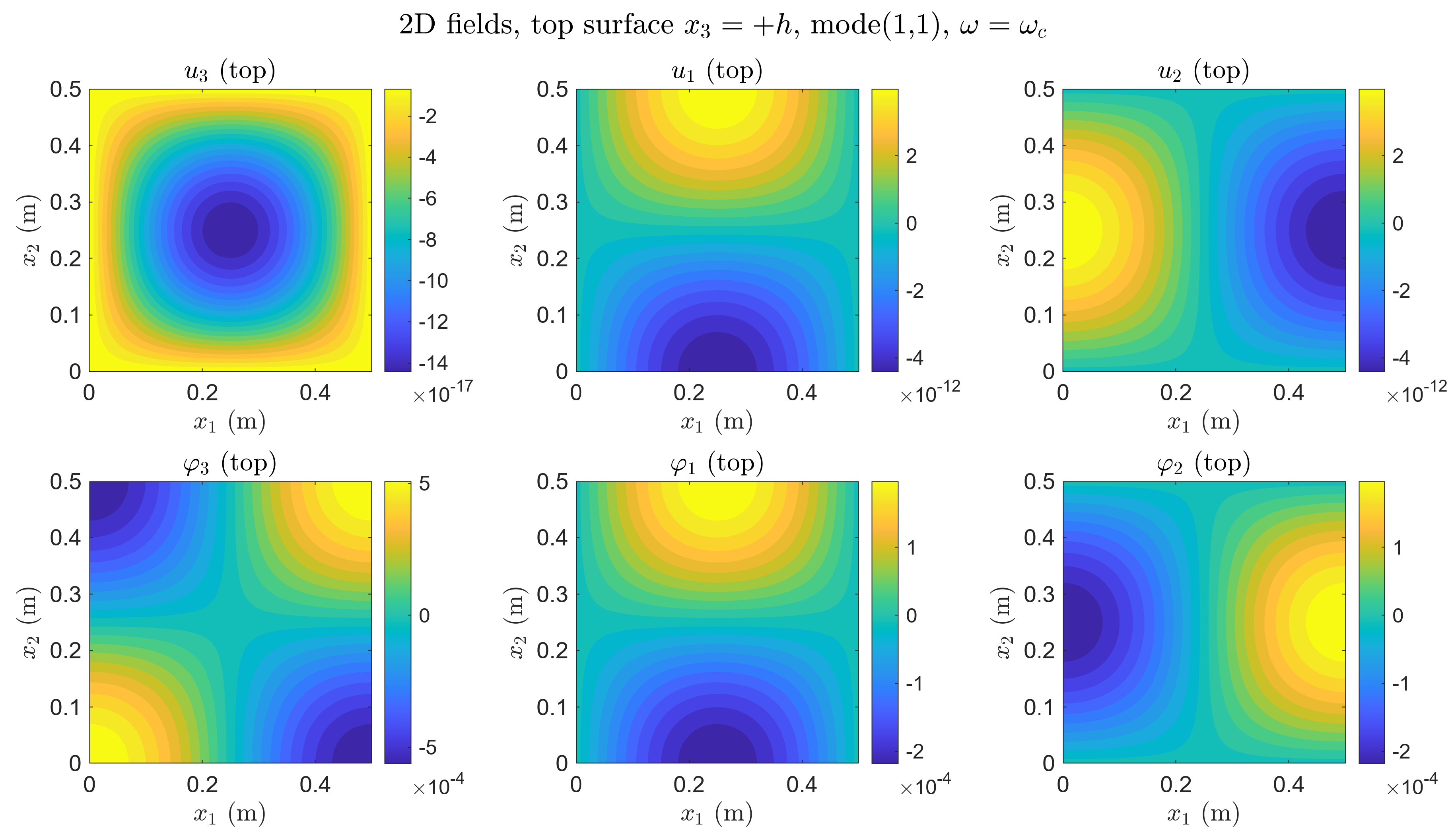
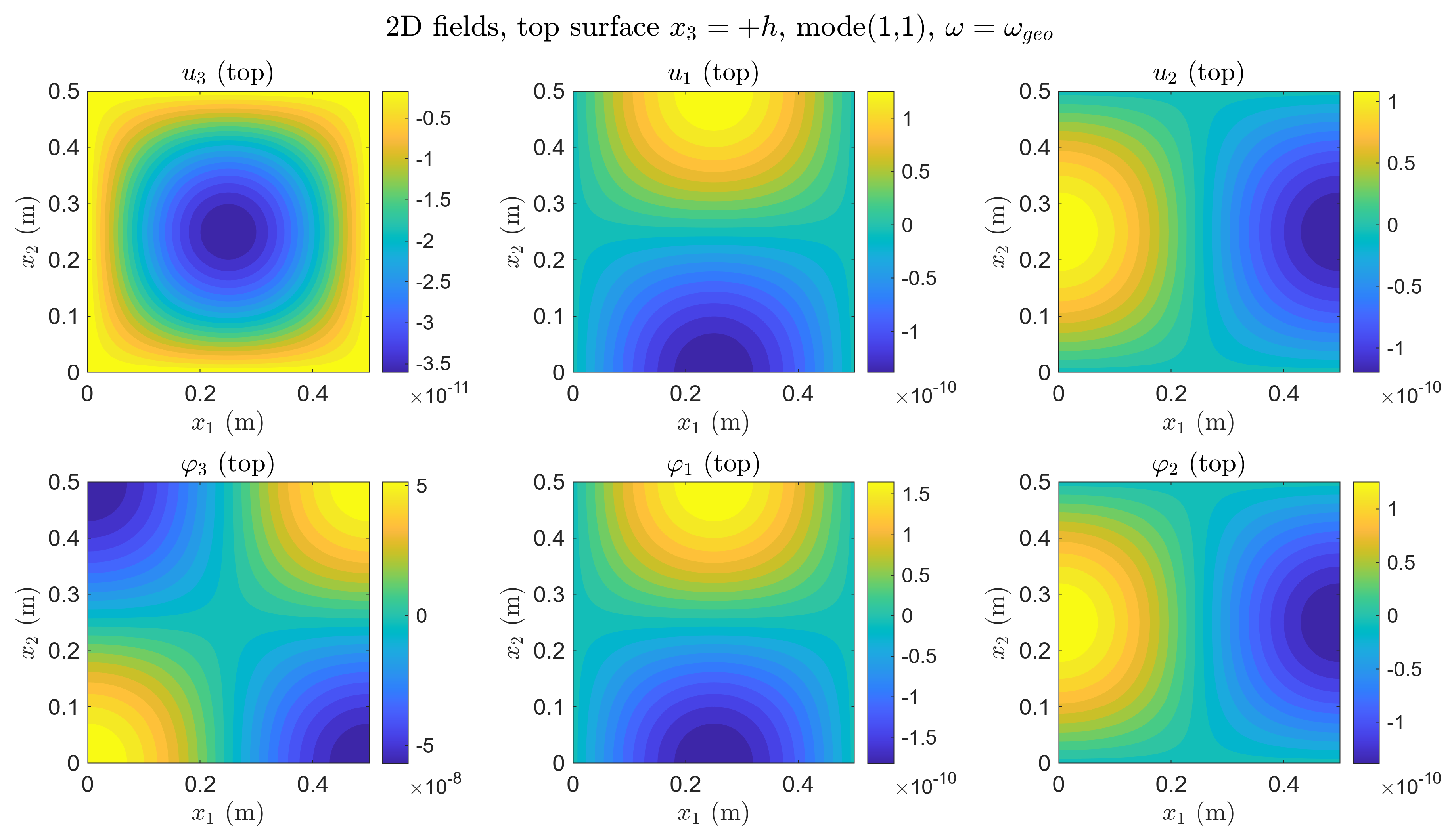
Figure A4.
Thickness profiles, first-order loads only. All profiles linear through zero at (antisymmetric). Bottom left—third panel (): slope sharply increases to ∼ at surface; slope negligible (∼). Bottom right—fourth panel (): largest slope; unchanged at ∼.
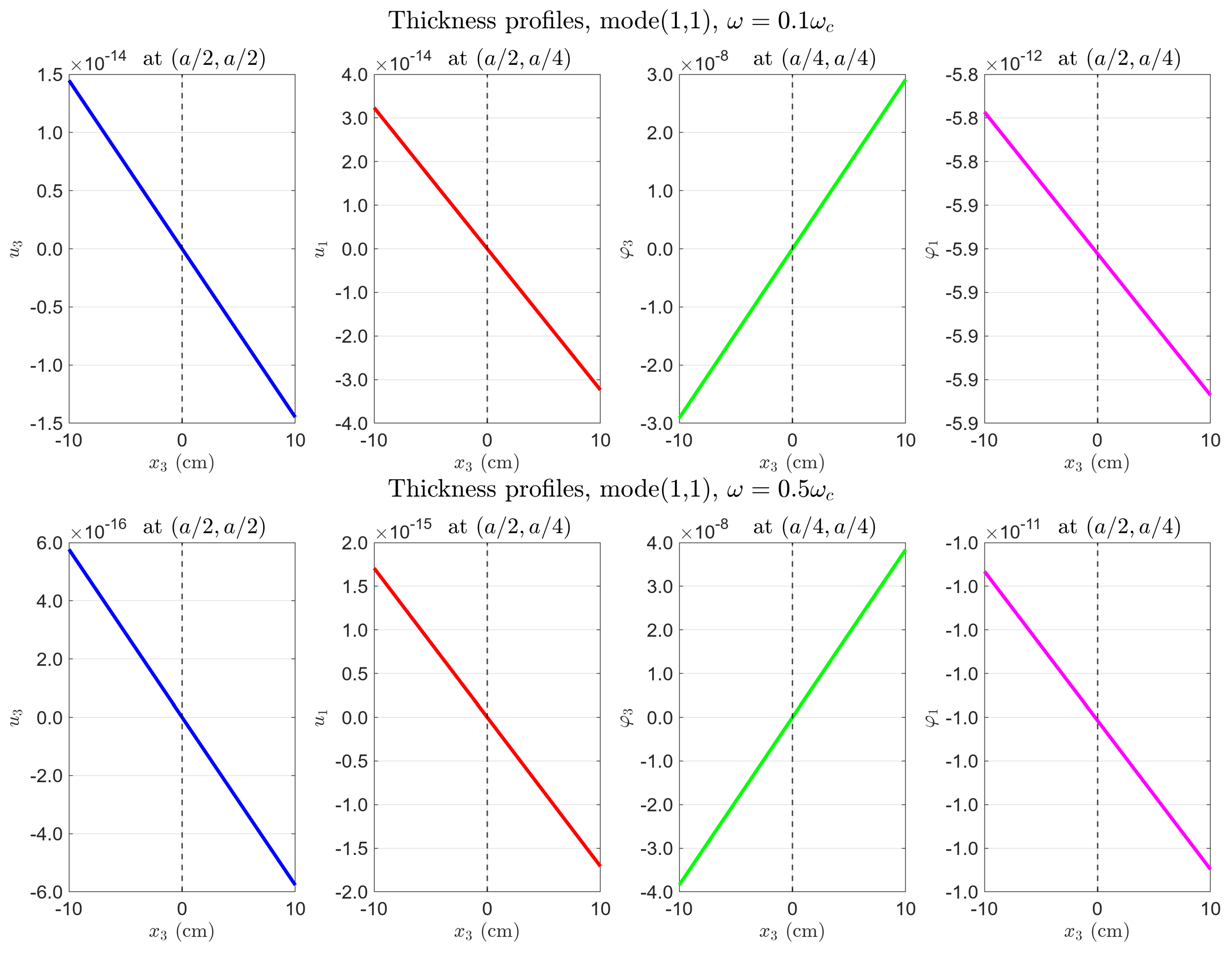
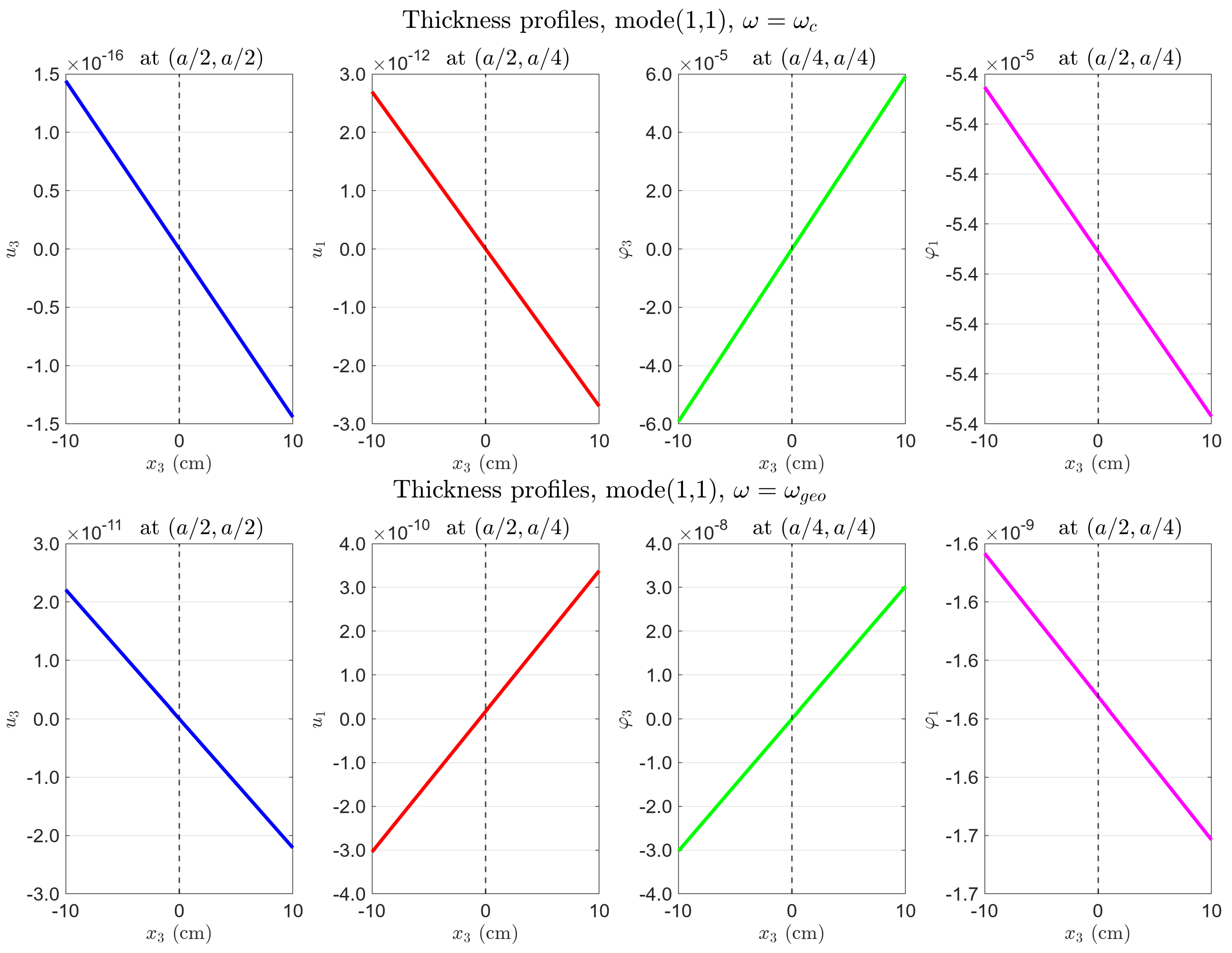
Figure A5.
Layer-by-layer fields along , first-order loads only. Layer curves cross at for all fields (antisymmetric profile). See Section 4.5.1 for physical interpretation.
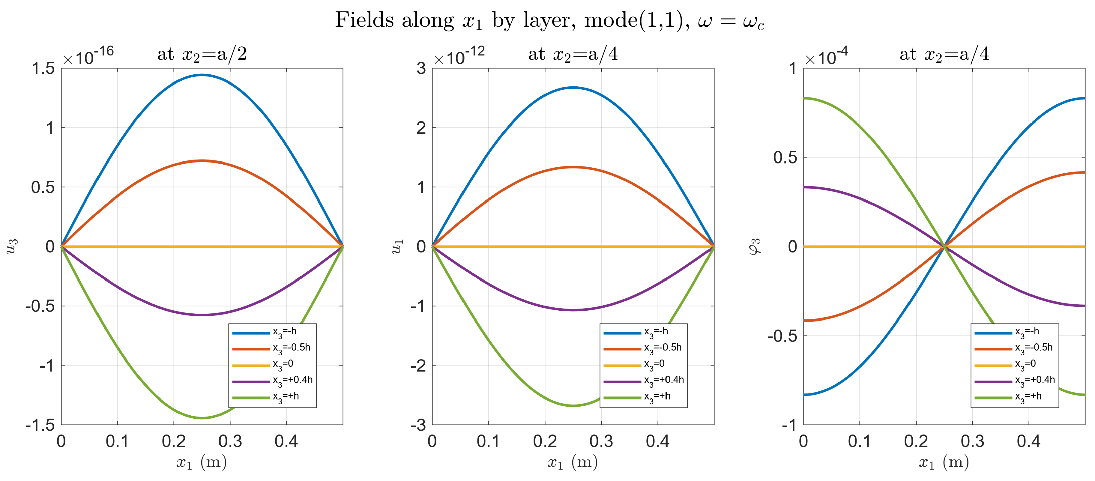
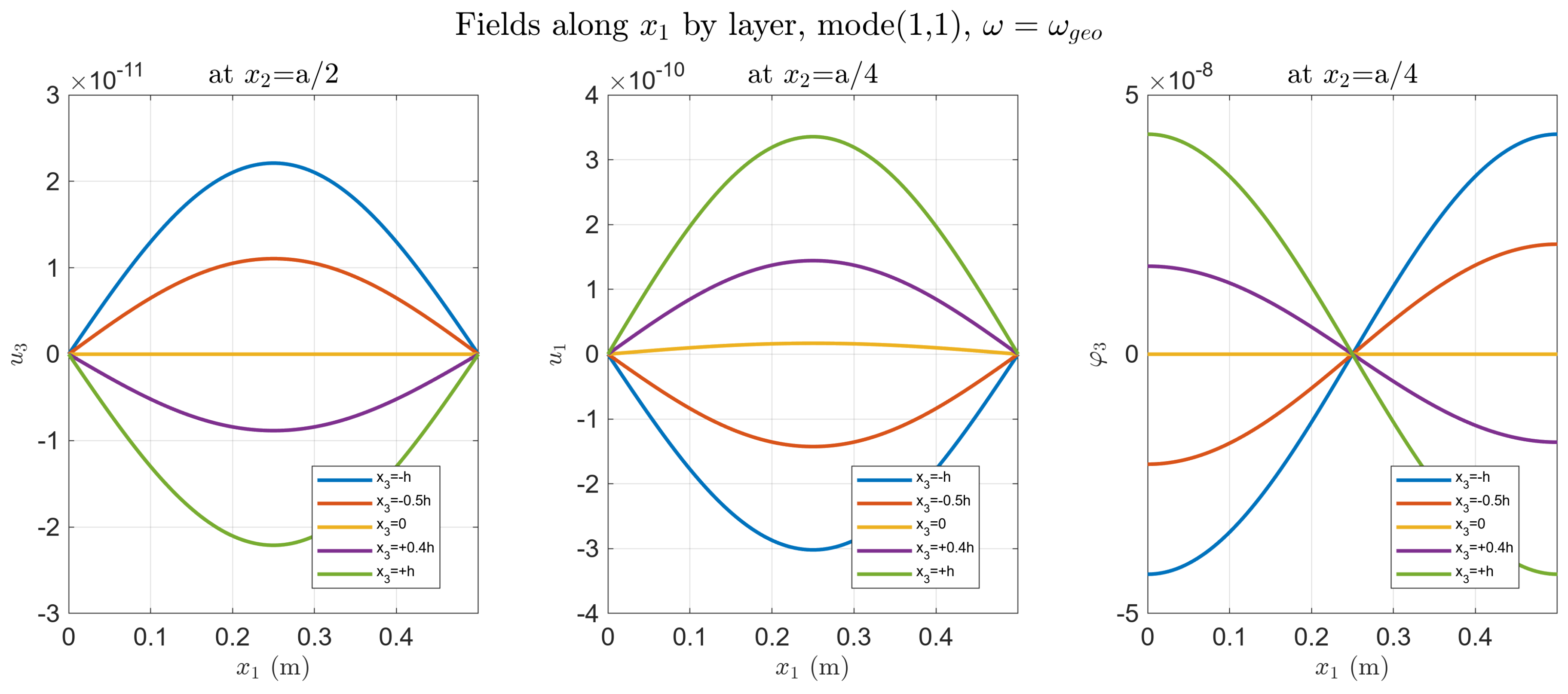
Figure A6.
Top surface , first-order loads only. (Upper) (): ∼ (bending rotation resonance); ∼ (locking). (Lower) (): at geometric resonance; ∼ (dead zone for rotation sensor).
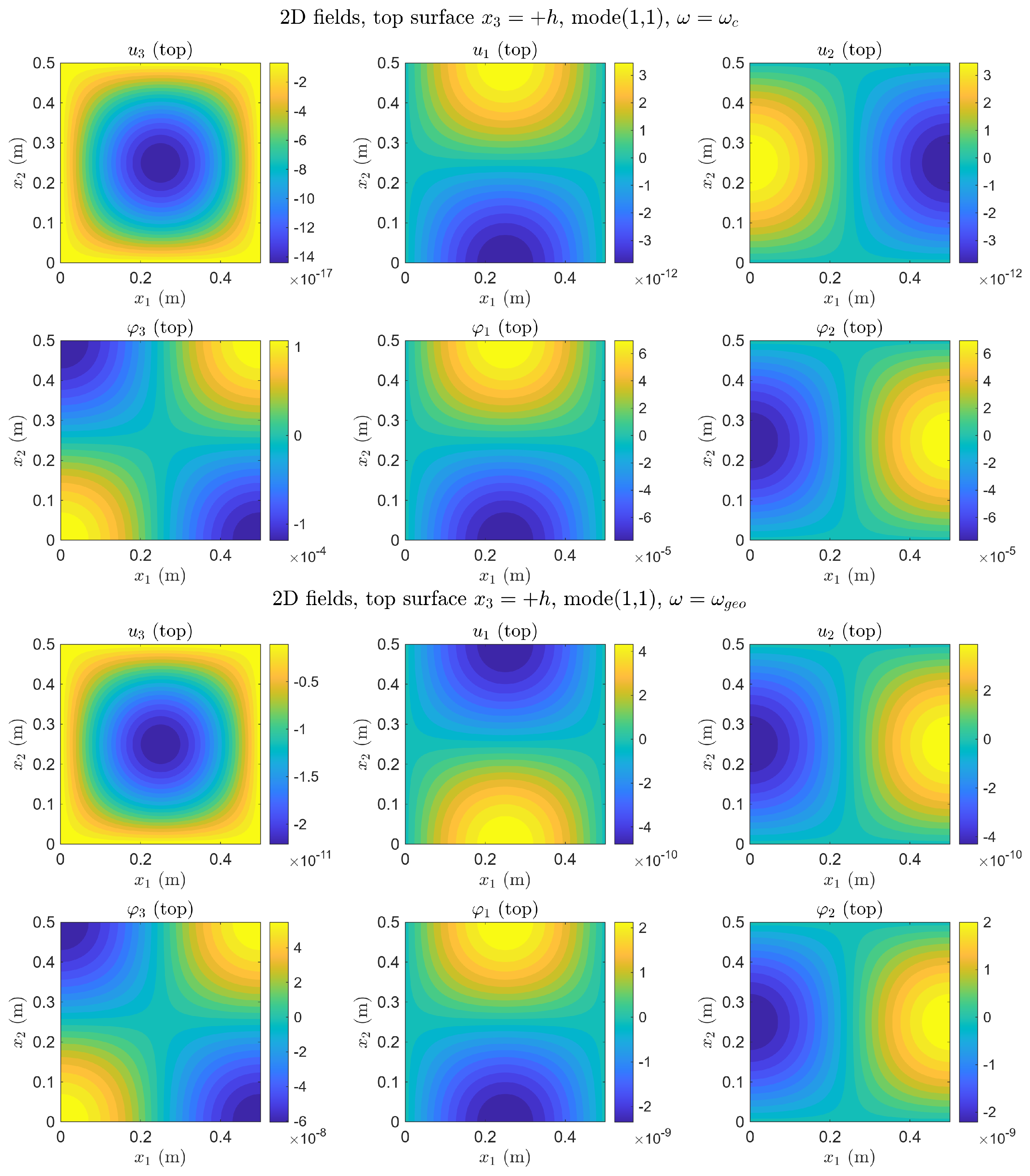
Figure A7.
Thickness profiles, all loads unity. Profiles linear, offset from zero at (S + A superposition). Bottom left—third panel (): ∼ at surface; ∼ (locking). Bottom right—fourth panel (): amplified; at quasi-static level.
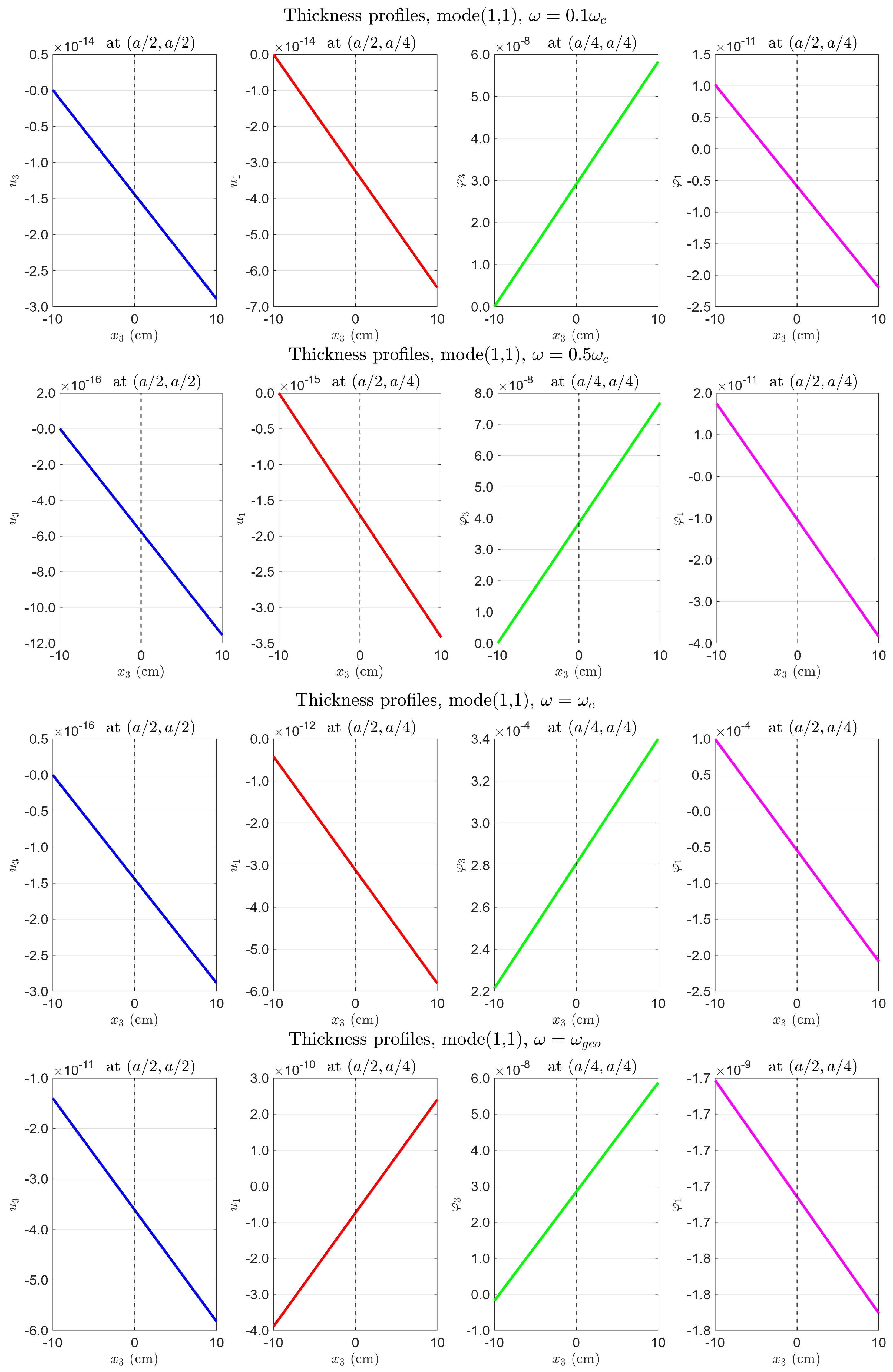
Figure A8.
Layer-by-layer fields along , all loads unity. Layer curves offset from zero (do not cross the axis): volume component present. See Section 4.5.1 for physical interpretation.
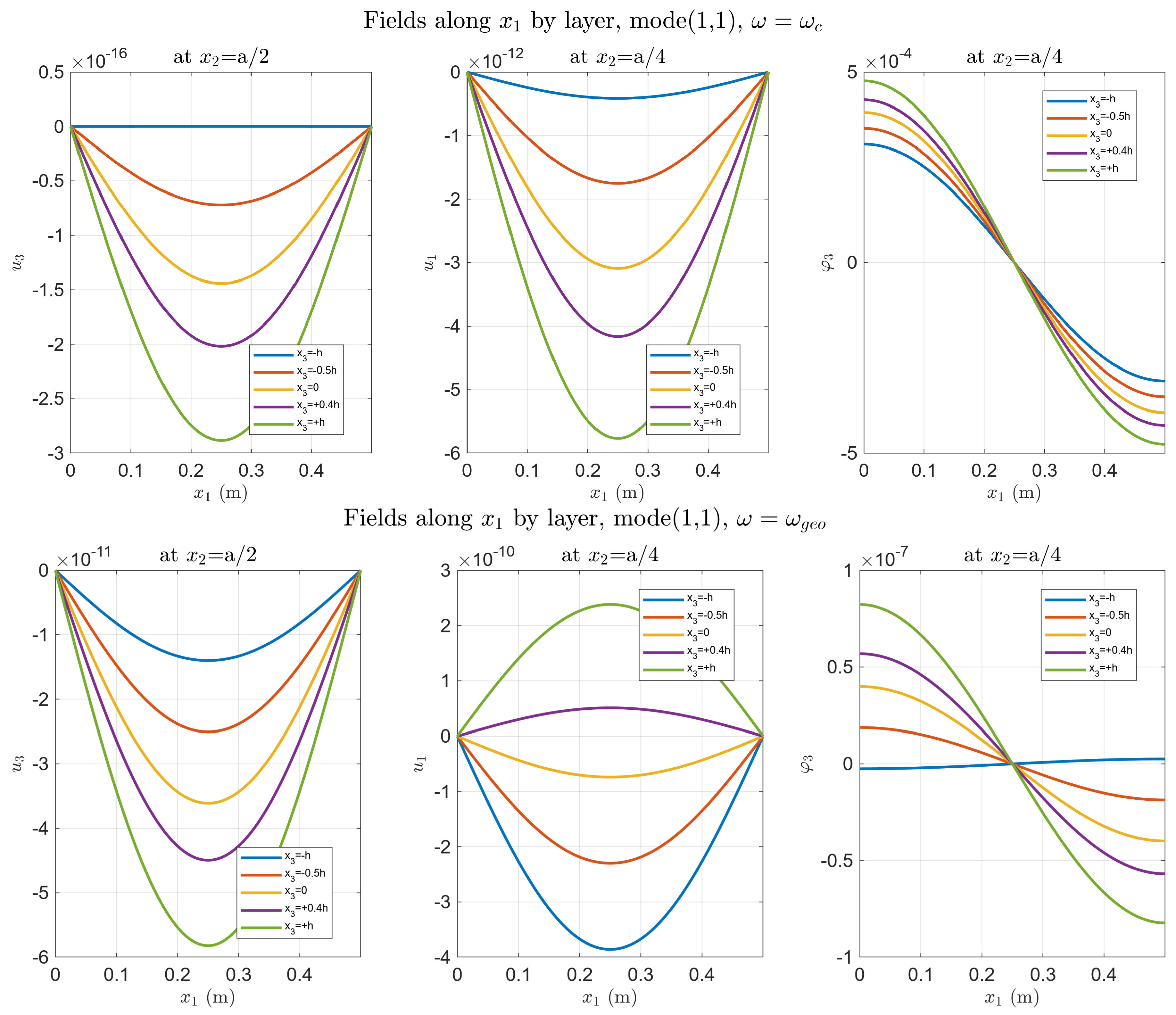
Figure A9.
Top surface , all loads unity. (Upper) (): ∼ (volume + bending resonance combined); ∼ (locking). (Lower) (): at geometric resonance; .
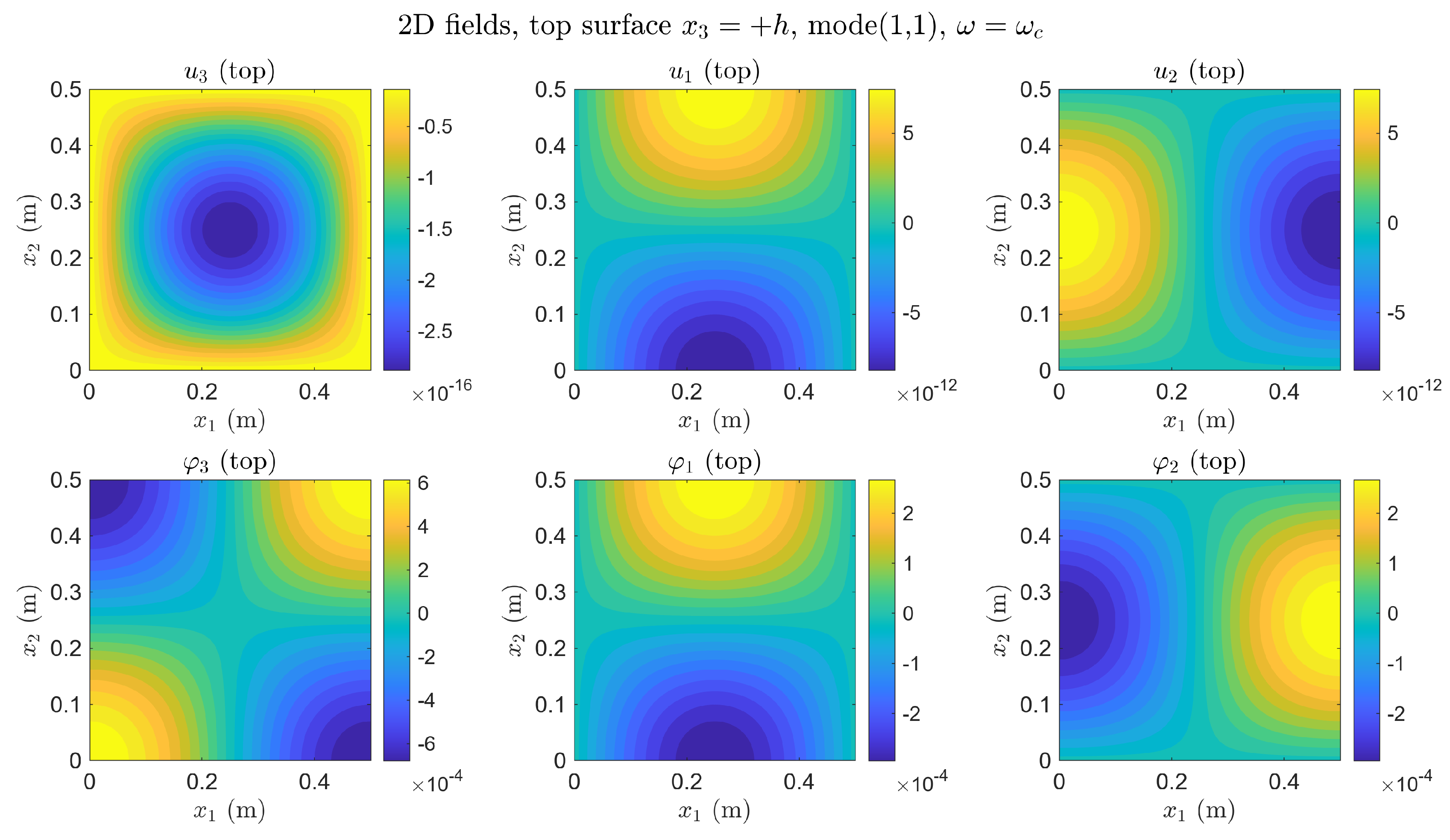
Appendix B.4. Reduced Coupling: , All Loads Unity
With , the material cutoff shifts to kHz, comparable to . The qualitative difference from B. 3 is the appearance of coupling between the two resonances (coupled regime, Section 4.6): at , the micro-rotation ∼, three orders above the standard- case, because the softer coupling allows the geometric resonance to excite indirectly. Displacement locking at persists unchanged (Figure A10, Figure A11 and Figure A12).
Figure A10.
Thickness profiles, , all loads unity. Bottom left—third panel (): locking persists (∼–, ∼). Bottom right—fourth panel (): ∼—three orders above Appendix B.3—coupled regime.
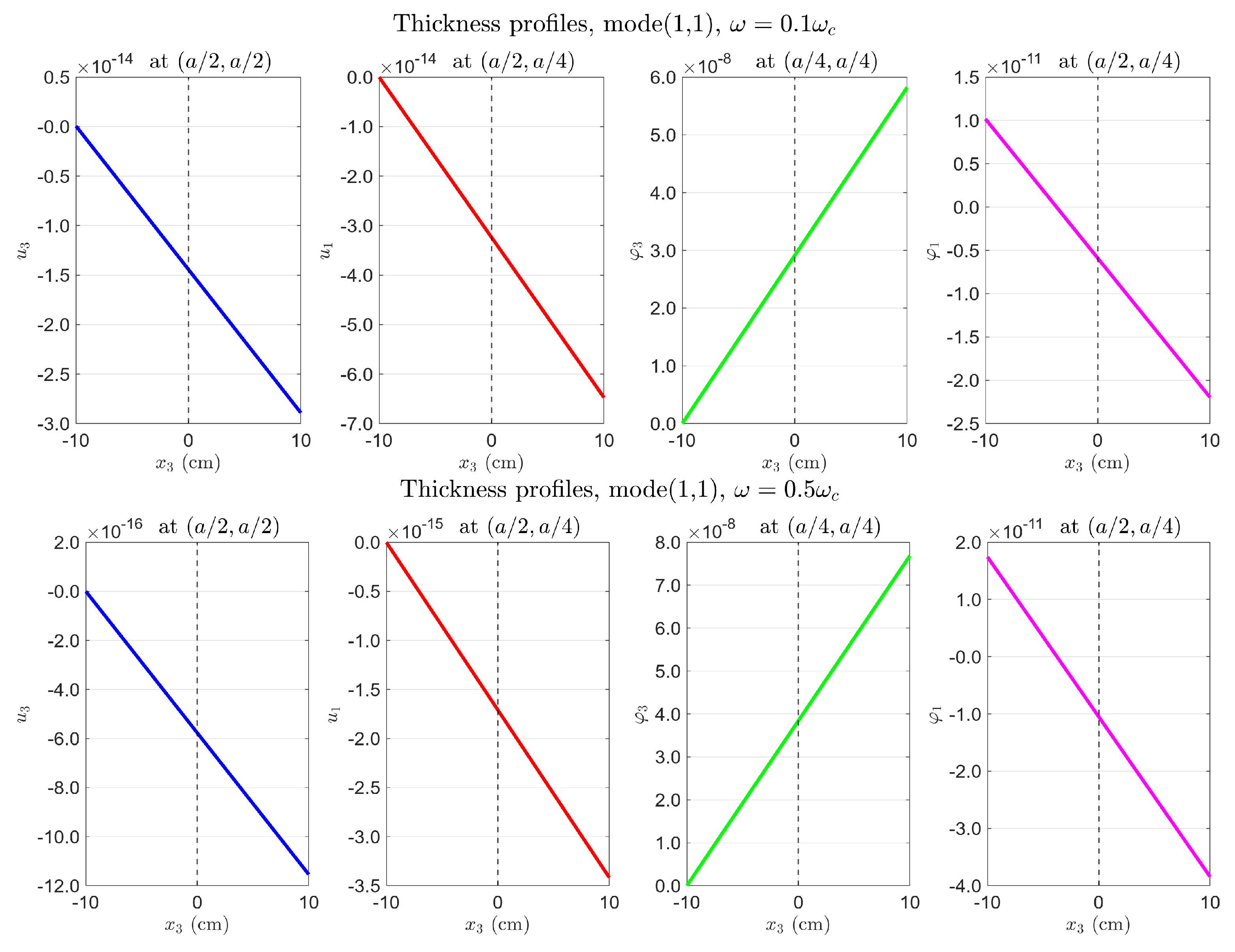
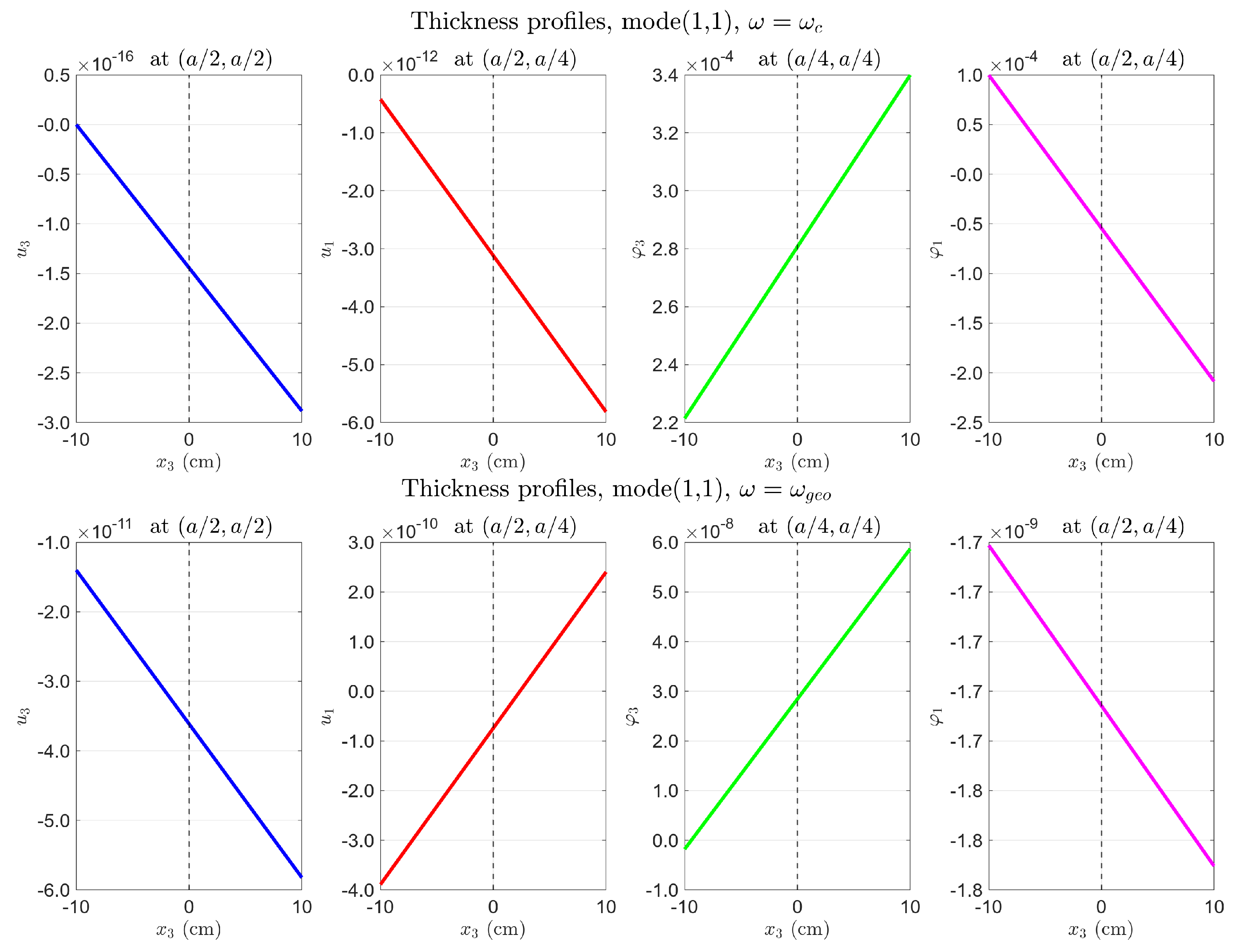
Figure A11.
Layer-by-layer fields, , all loads unity. Layer separation in at markedly increased relative to Appendix B.3. See Section 4.5.1 for physical interpretation.
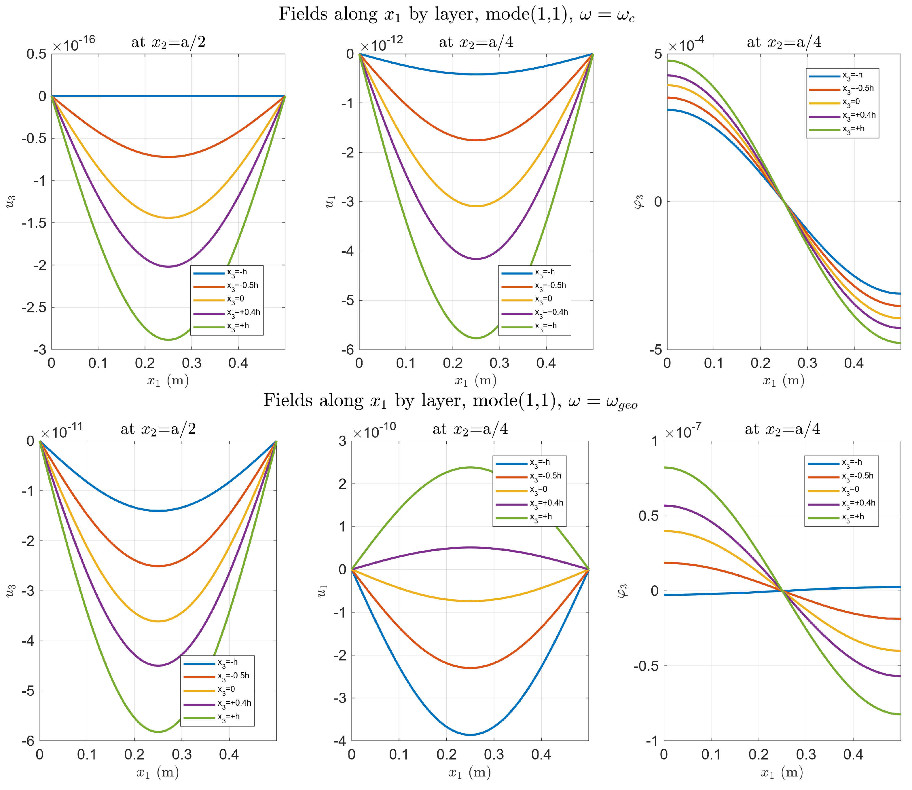
Figure A12.
Top surface , , all loads unity. (Upper) ( kHz): ∼; ∼ (locking). (Lower) (): ∼ (coupled regime—compare with Appendix B.3 right: ).
References
- Lakes, R.S. Experimental microelasticity of two porous solids. Int. J. Solids Struct. 1986, 22, 55–63. [Google Scholar] [CrossRef] [Scilit]
- Ulukhanyan, A.; Misra, A. A second-degree micromorphic continuum model for 1D granular structures. Math. Mech. Solids. 2026. [Google Scholar] [CrossRef] [Scilit]
- Koenders, M.A. Wave propagation through elastic granular and granular auxetic materials. Phys. Status Solidi B 2009, 246, 2083–2088. [Google Scholar] [CrossRef] [Scilit]
- Yang, F.; Munroe, M.J. Experimental study of micropolar and couple stress elasticity in compact bone in bending. J. Biomech. 1982, 15, 91–98. [Google Scholar] [CrossRef] [Scilit] [PubMed]
- Karttunen, A.T.; Reddy, J.N.; Romanoff, J. Two-scale micropolar plate model for web-core sandwich panels. Int. J. Solids Struct. 2019, 170, 82–94. [Google Scholar] [CrossRef] [Scilit]
- Cosserat, E.; Cosserat, F. Théorie des Corps Déformables; A. Hermann et fils: Paris, France, 1909. [Google Scholar]
- Eringen, A.C. Theory of Micropolar Elasticity; Springer: New York, NY, USA, 1999. [Google Scholar]
- Nowacki, W. Theory of Micropolar Elasticity; CISM International Centre for Mechanical Sciences (CISM); Springer: Vienna, Austria, 1986; Volume 25. [Google Scholar] [CrossRef] [Scilit]
- Mindlin, R.D.; Tiersten, H.F. Effects of couple-stresses in linear elasticity. Arch. Ration. Mech. Anal. 1962, 11, 415–448. [Google Scholar] [CrossRef] [Scilit]
- Mindlin, R.D. Micro-structure in linear elasticity. Arch. Ration. Mech. Anal. 1964, 16, 51–78. [Google Scholar] [CrossRef] [Scilit]
- Rizzi, G.; d’Agostino, M.V.; Neff, P.; Madeo, A. Boundary and interface conditions in the relaxed micromorphic model: Exploring finite-size metastructures for elastic wave control. Math. Mech. Solids 2022, 27, 1053–1068. [Google Scholar] [CrossRef] [Scilit]
- Rizzi, G.; Tallarico, D.; Neff, P.; Madeo, A. Towards the conception of complex engineering meta-structures: Relaxed-micromorphic modelling of low-frequency mechanical diodes/high-frequency screens. Wave Motion 2022, 113, 102920. [Google Scholar] [CrossRef] [Scilit]
- Ogam, E.; Fellah, Z.E.A.; Fellah, M.; Depollier, C. Theoretical and experimental study of micropolar elastic materials using acoustic waves in air. J. Sound Vib. 2021, 510, 116298. [Google Scholar] [CrossRef] [Scilit]
- Singh, S.K.; Varma, R.K.; Banerjee, A.; Rathore, K.K. Study of wave motion on the emergence of veering, locking, and coupling in periodic composite panels. J. Acoust. Soc. Am. 2024, 155, 826–836. [Google Scholar] [CrossRef] [Scilit] [PubMed]
- Rao, K.M. Longitudinal wave propagation in a micropolar wave guide. Int. J. Eng. Sci. 1988, 26, 135–141. [Google Scholar] [CrossRef] [Scilit]
- Lakes, R.S. Experimental evaluation of micromorphic elastic constants in foams and lattices. Z. Angew. Math. Phys. 2023, 74, 31. [Google Scholar] [CrossRef] [Scilit]
- Xu, Y.; Mao, M.; Huang, X.H.; Guo, Y.Q.; Yang, Y.; Dong, Y.R.; Shah, S.A.A.; Gao, X.; Usman, M.; Jeong, S.H. Comparative investigation of dynamic damping and fracture in viscoelastic dampers with two different interfacial bonding types: Molecular dynamics simulations and device tests. J. Build. Eng. 2025, 116, 114582. [Google Scholar] [CrossRef] [Scilit]
- Ulukhanyan, A. Modeling of Deformation of Micropolar Prismatic Thin Bodies Using the Legendre Polynomial System. Ph.D. Thesis, Moscow Aviation Institute, Moscow, Russia, 2012. (In Russian) [Google Scholar]
- Ulukhanyan, A. Dispersion equations and wave velocities in micropolar theory of elasticity. Lobachevskii J. Math. 2024, 45, 3773–3782. [Google Scholar] [CrossRef] [Scilit]
- Nikabadze, M.; Ulukhanyan, A. On the decomposition of equations of micropolar elasticity and thin body theory. Lobachevskii J. Math. 2020, 41, 2059–2074. [Google Scholar] [CrossRef] [Scilit]
- Nikabadze, M.; Ulukhanyan, A. On some variational principles in micropolar theories of single-layer thin bodies. Contin. Mech. Thermodyn. 2023, 35, 1147–1164. [Google Scholar] [CrossRef] [Scilit]
- Nikabadze, M.; Ulukhanyan, A. Mathematical modeling of elastic thin bodies with one small size. In Higher Gradient Materials and Related Generalized Continua; Advanced Structured Materials; Altenbach, H., Müller, W., Abali, B., Eds.; Springer: Cham, Switzerland, 2019; Volume 120, pp. 155–199. [Google Scholar] [CrossRef] [Scilit]
- Nikabadze, M. Development of the Method of Orthogonal Polynomials in the Mechanics of Micropolar and Classical Elastic Thin Bodies; Moscow University Press: Moscow, Russia, 2023. [Google Scholar]
- Ulukhanyan, A. Micropolar prismatic body in the first approximation: Bending, coupled dispersion, and analytical shear correction factor. ZAMM-J. Appl. Math. Mech. 2026. under review. [Google Scholar] [CrossRef] [Scilit]
- Ulukhanyan, A. Zero approximation of micropolar prismatic bodies via Legendre polynomial expansion: Dispersion and wave phenomena. Contin. Mech. Thermodyn. 2026. [Google Scholar] [CrossRef] [Scilit]
- Gharahi, A. Boundary value problems in a theory of bending of thin micropolar plates with surface elasticity. J. Elast. 2024, 156, 307–324. [Google Scholar] [CrossRef] [Scilit]
- Sarhil, M.; Scheunemann, L.; Schröder, J.; Neff, P. Modeling the size-effect of metamaterial beams under bending via the relaxed micromorphic continuum. Proc. Appl. Math. Mech. 2023, 22, e202200033. [Google Scholar] [CrossRef] [Scilit]
- Alberdi, R.; Robbins, J.; Walsh, T.; Dingreville, R. Exploring wave propagation in heterogeneous metastructures using the relaxed micromorphic model. J. Mech. Phys. Solids 2021, 155, 104540. [Google Scholar] [CrossRef] [Scilit]
- Papa Dukić, E.; Grbac, L.; Jelenić, G. Characteristic bending length in micropolar materials with periodic internal structure. J. Mech. Mater. Struct. 2024, 19, 515–530. [Google Scholar] [CrossRef] [Scilit]
- Meso, C.; Franklin, H.; Ogam, E.; Fellah, Z.A. Micropolar elastic materials: Insights from transmitted acoustic wave analysis. In Proceedings of the 17e Congrès Français d’Acoustique, Paris, France, 27–30 April 2025. hal-05219880. [Google Scholar]
- Fedele, R.; Placidi, L.; Fabbrocino, F. A review of inverse problems for generalized elastic media: Formulations, experiments, synthesis. Contin. Mech. Thermodyn. 2024, 36, 1413–1453. [Google Scholar] [CrossRef] [Scilit]
- Rose, J.L. Ultrasonic Guided Waves in Solid Media; Cambridge University Press: Cambridge, UK, 2014; p. 512. [Google Scholar] [CrossRef] [Scilit]
- Gharehbaghi, V.R.; Noroozinejad Farsangi, E.; Noori, M.; Yang, T.Y.; Li, S.; Nguyen, A.; Málaga-Chuquitaype, C.; Gardoni, P.; Mirjalili, S. A critical review on structural health monitoring: Definitions, methods, and perspectives. Arch. Comput. Methods Eng. 2022, 29, 2209–2235. [Google Scholar] [CrossRef] [Scilit]
- Wu, W.; Cantero-Chinchilla, S.; Yan, W.J.; Chiachio Ruano, M.; Remenyte-Prescott, R.; Chronopoulos, D. Damage quantification and identification in structural joints through ultrasonic guided wave-based features and an inverse Bayesian scheme. Sensors 2023, 23, 4160. [Google Scholar] [CrossRef] [Scilit] [PubMed]
- Ricci, F.; Monaco, E.; Boffa, N.D.; Maio, L.; Memmolo, V. Guided waves for structural health monitoring in composites: A review and implementation strategies. Prog. Aerosp. Sci. 2022, 129, 100790. [Google Scholar] [CrossRef] [Scilit]
- Colatosti, M.; Carboni, B.; Fantuzzi, N.; Trovalusci, P. Composite material identification as micropolar continua via an optimization approach. Compos. Part C Open Access 2023, 11, 100362. [Google Scholar] [CrossRef] [Scilit]
- Kachanov, L.M. Rupture Time Under Creep Conditions. Int. J. Fract. 1999, 97, 11–18. [Google Scholar] [CrossRef] [Scilit]
- Kachanov, L.M. Introduction to Continuum Damage Mechanics; Mechanics of Elastic Stability Series; Springer: Dordrecht, The Netherlands, 1986. [Google Scholar] [CrossRef] [Scilit]
- Rabotnov, Y.N. Creep rupture. In Applied Mechanics; Hetényi, M., Vincenti, W.G., Eds.; Springer: Berlin/Heidelberg, Germany, 1969; pp. 342–349. [Google Scholar] [CrossRef] [Scilit]
- Lemaitre, J.; Chaboche, J.L. Mechanics of Solid Materials; Cambridge University Press: Cambridge, UK, 1990. [Google Scholar]
- Krajcinovic, D. Damage Mechanics; Elsevier: Amsterdam, The Netherlands, 1996; Volume 41. [Google Scholar]
- Thatipelli, K.R.; Kalathur, H.; Gouripriya, S. Size-dependent mechanics in finite cellular lattices: Structural and Cosserat responses under tension and bending. Int. J. Solids Struct. 2026, 326, 113750. [Google Scholar] [CrossRef] [Scilit]
- Vekua, I.N. Some General Methods of Constructing Various Variants of the Theory of a Shell; Nauka: Moscow, Russia, 1982; p. 286. [Google Scholar]
- Nikabadze, M.U.; Ulukhanyan, A.R. Analytical Solutions in the Theory of Thin Bodies. In Generalized Continua as Models for Classical and Advanced Materials; Advanced Structured Materials; Altenbach, H., Forest, S., Eds.; Springer: Cham, Switzerland, 2016; Volume 42. [Google Scholar] [CrossRef] [Scilit]
- Ulukhanyan, A. Dynamic equations of the theory of thin prismatic bodies with expansion in the system of Legendre polynomials. Mech. Solids 2011, 46, 467–479. [Google Scholar] [CrossRef] [Scilit]
- Mindlin, R.D. Influence of rotatory inertia and shear on flexural motions of isotropic, elastic plates. J. Appl. Mech. 1951, 18, 31–38. [Google Scholar] [CrossRef] [Scilit]
- Reissner, E. The effect of transverse shear deformation on the bending of elastic plates. J. Appl. Mech. 1945, 12, A69–A77. [Google Scholar] [CrossRef] [Scilit]
- Eringen, A.C. Microcontinuum Field Theories; Springer: New York, NY, USA, 1999. [Google Scholar] [CrossRef] [Scilit]
- Aifantis, E.C. On the role of gradients in the localization of deformation and fracture. Int. J. Eng. Sci. 1992, 30, 1279–1299. [Google Scholar] [CrossRef] [Scilit]
- Steinberg, L.; Kvasov, R. Enhanced mathematical model for Cosserat plate bending. Thin-Walled Struct. 2013, 63, 51–62. [Google Scholar] [CrossRef] [Scilit]
- Leissa, A.W. On a curve veering aberration. J. Appl. Math. Phys. ZAMP 1974, 25, 99–111. [Google Scholar] [CrossRef] [Scilit]
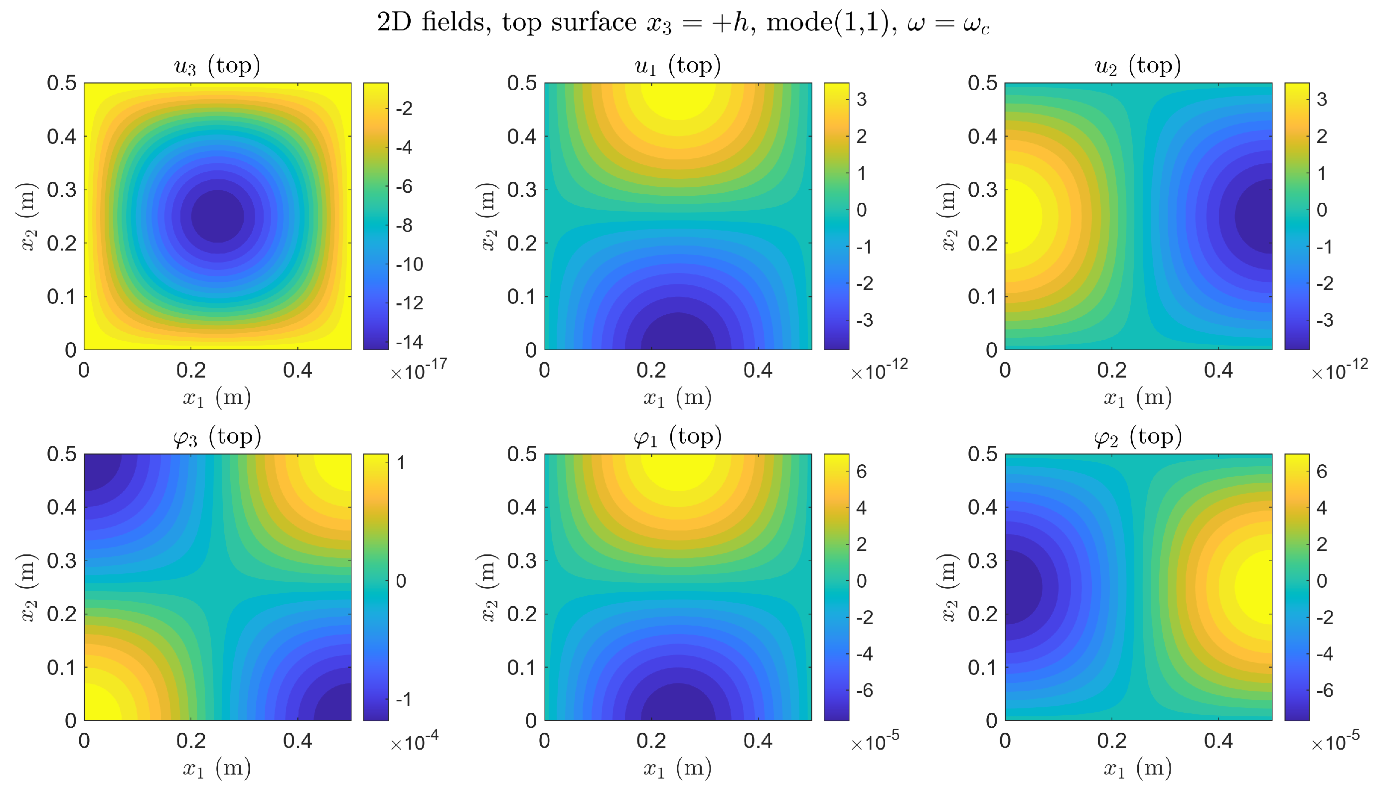
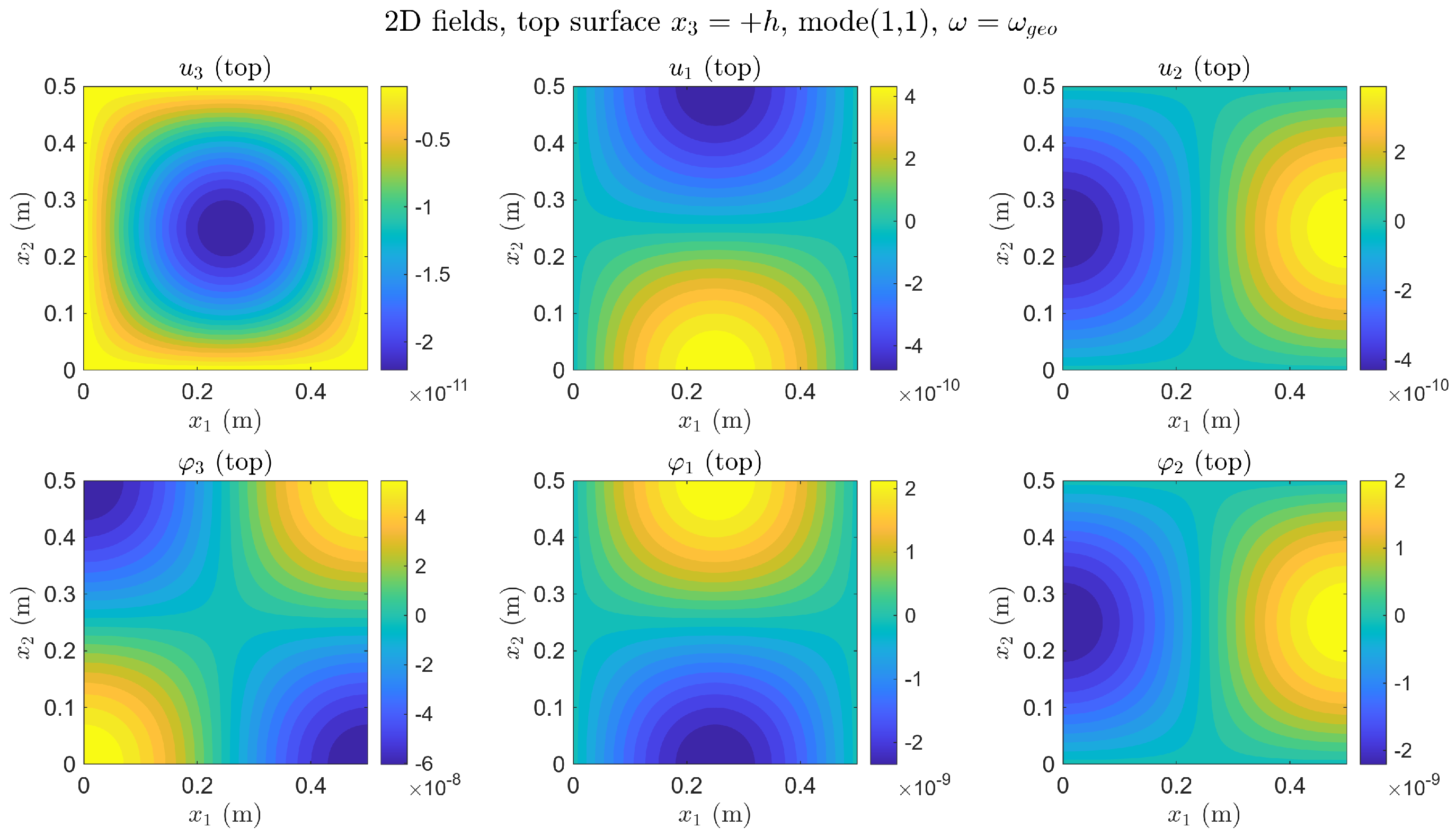
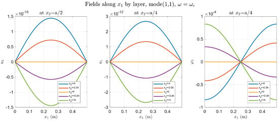
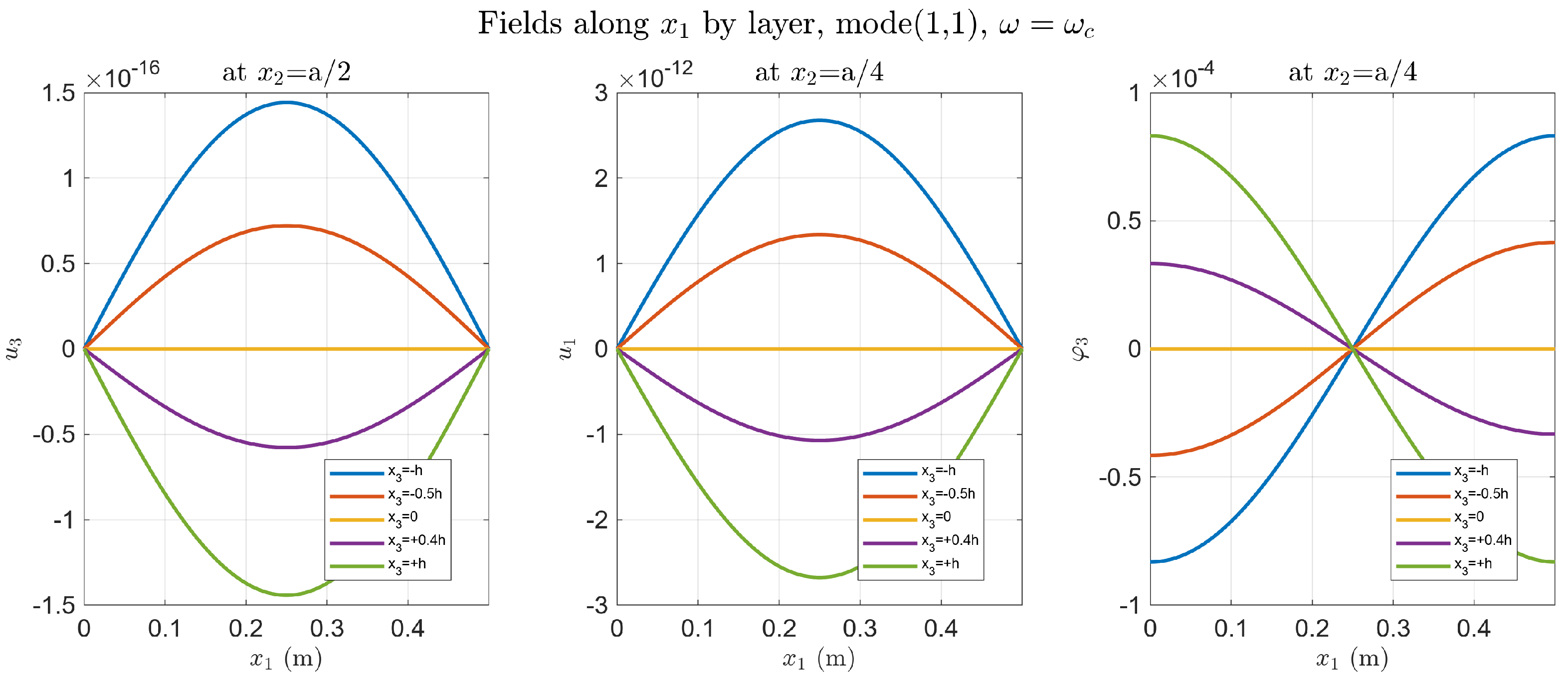
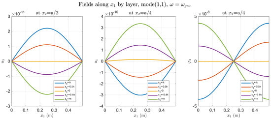
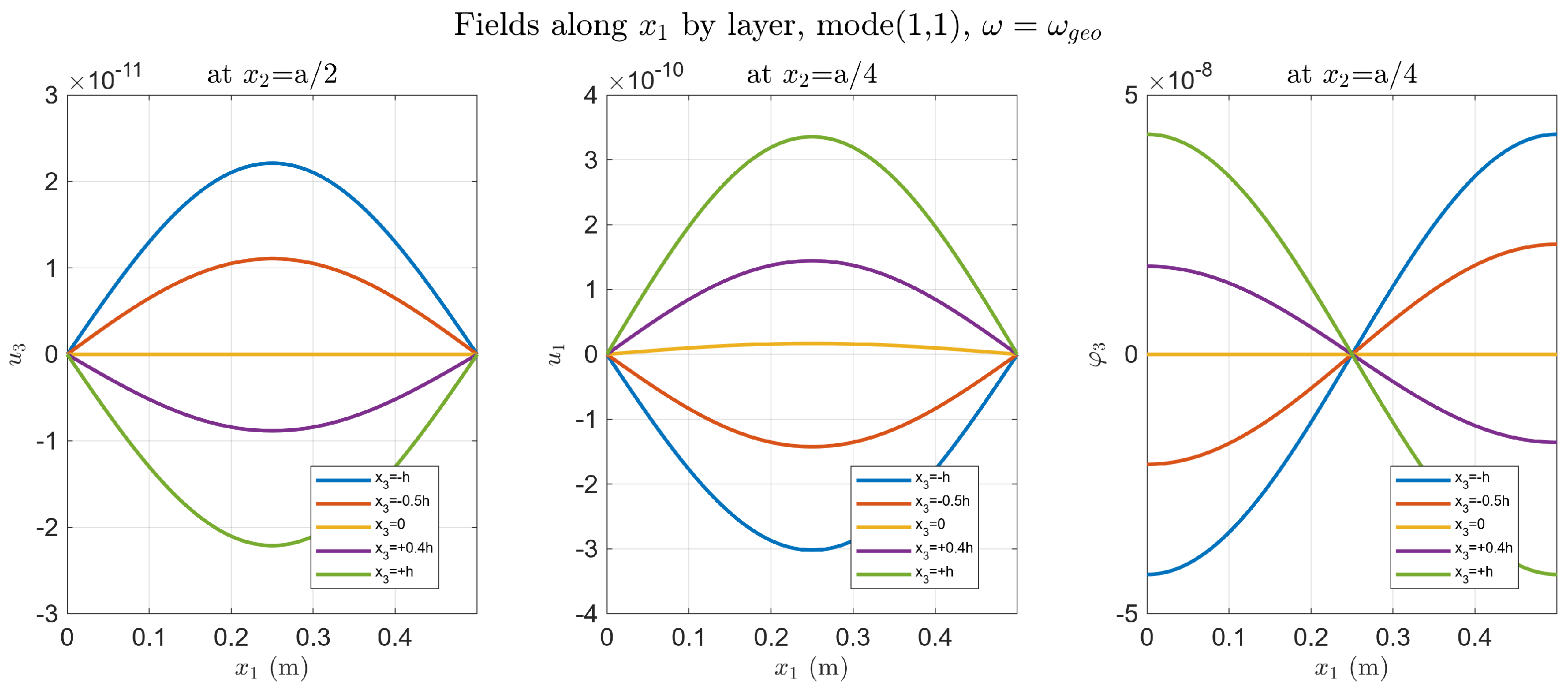
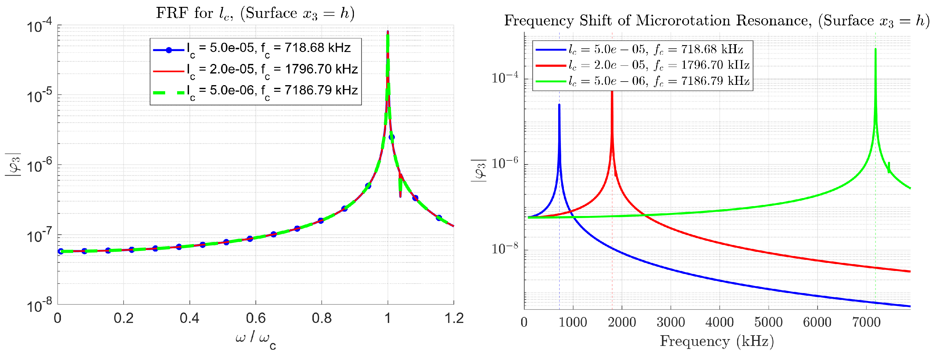
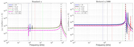
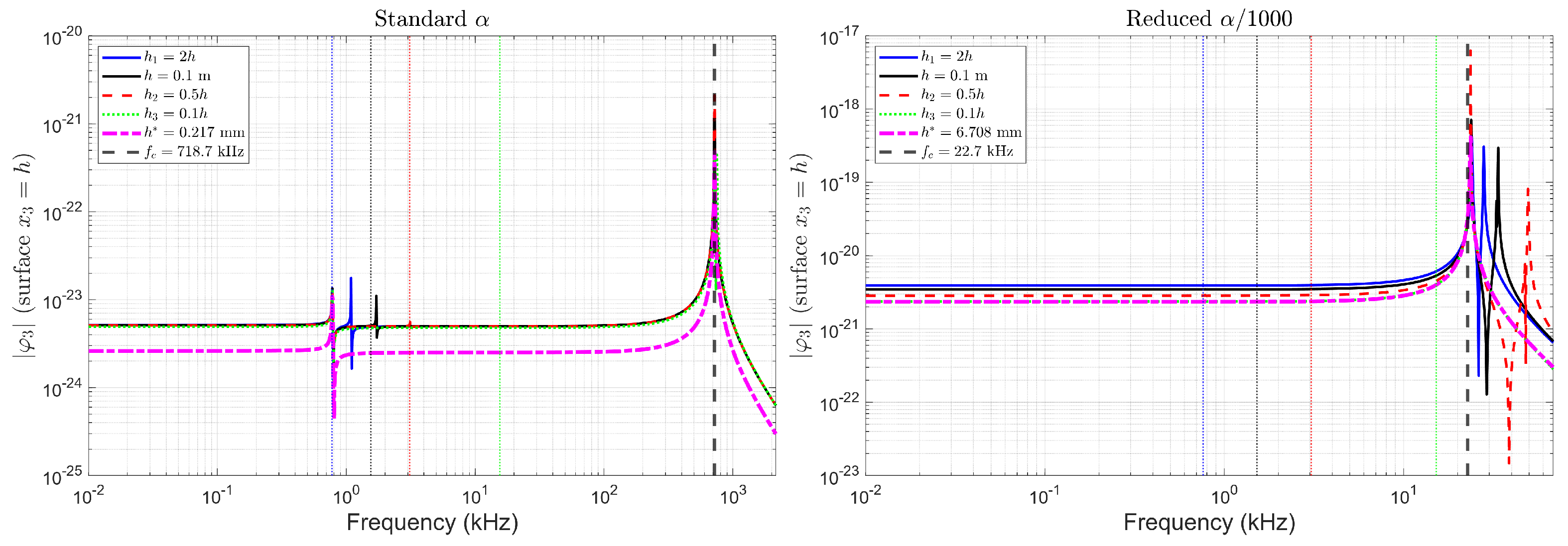
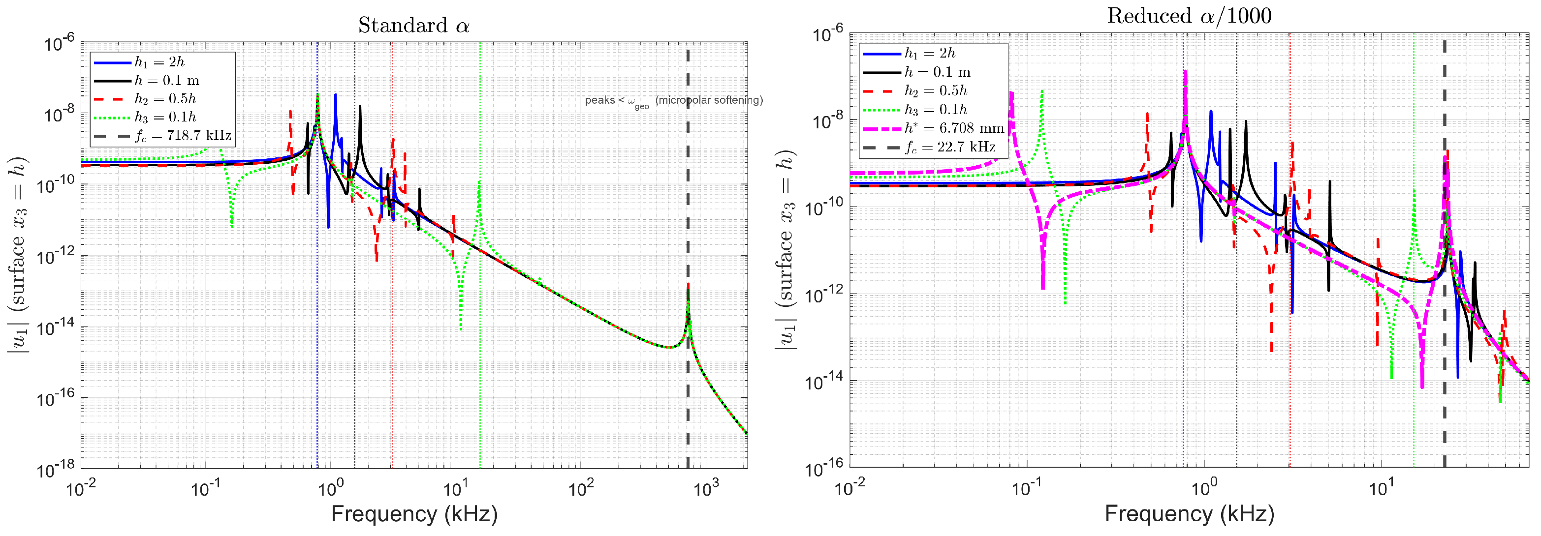
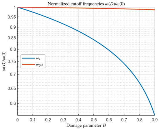
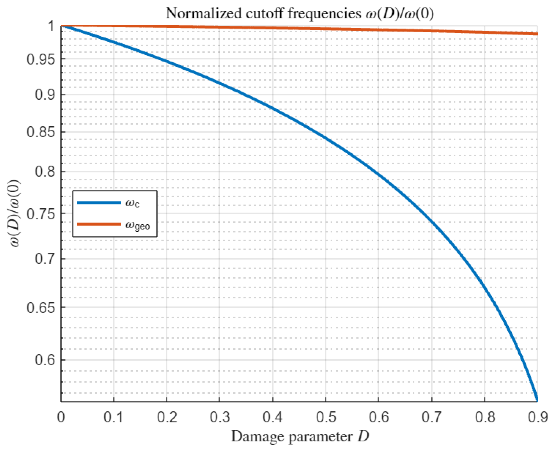
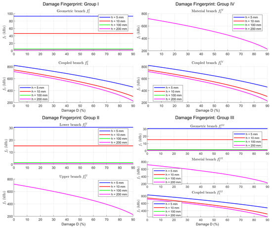
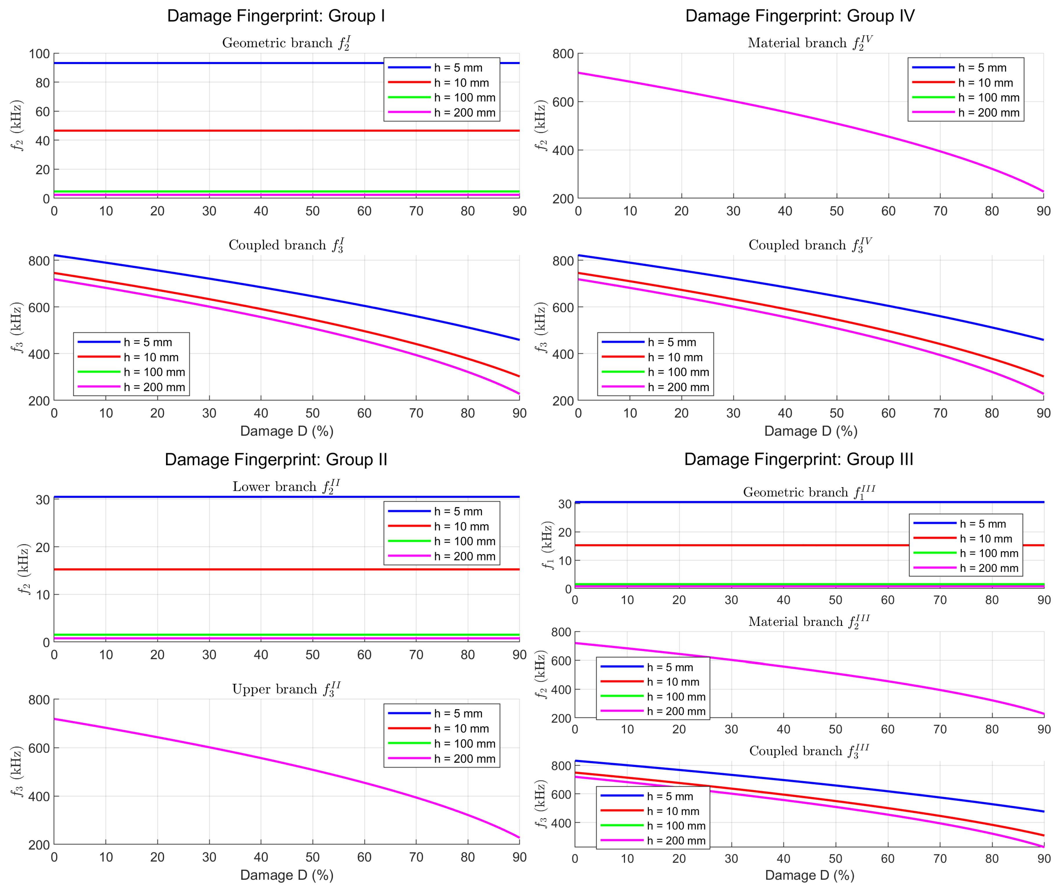
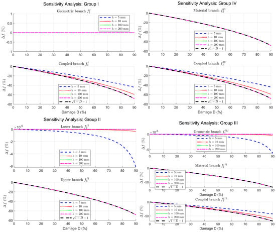
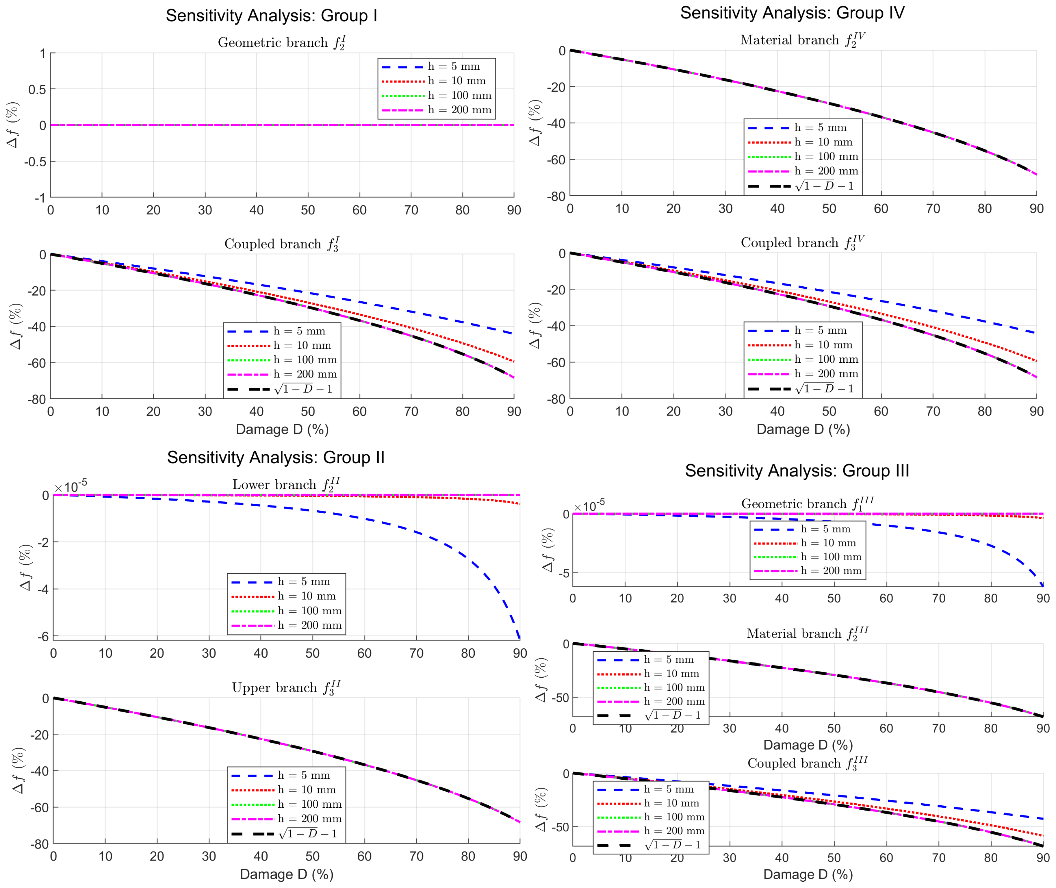
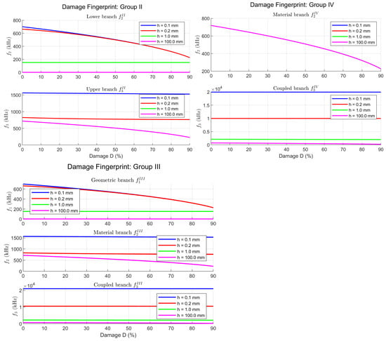
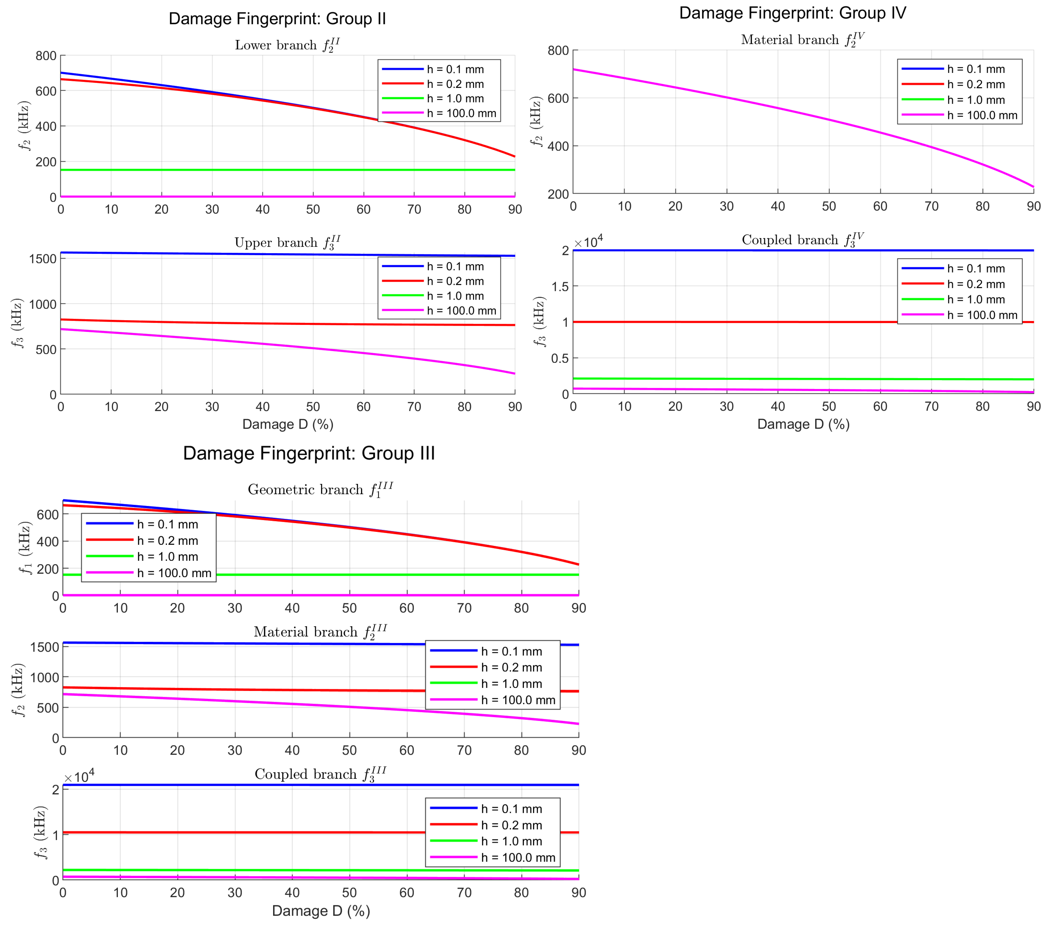
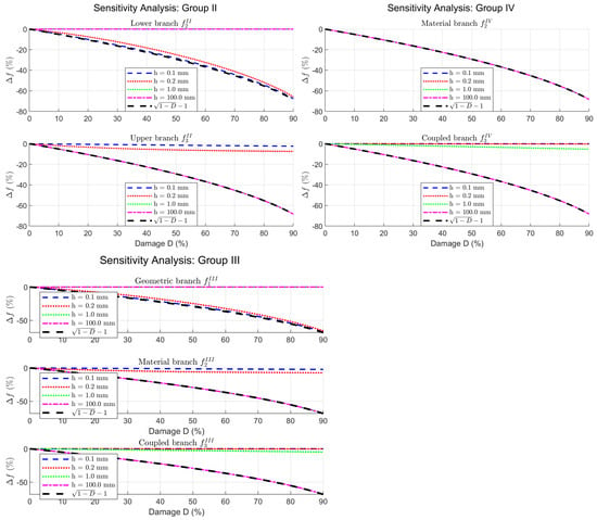
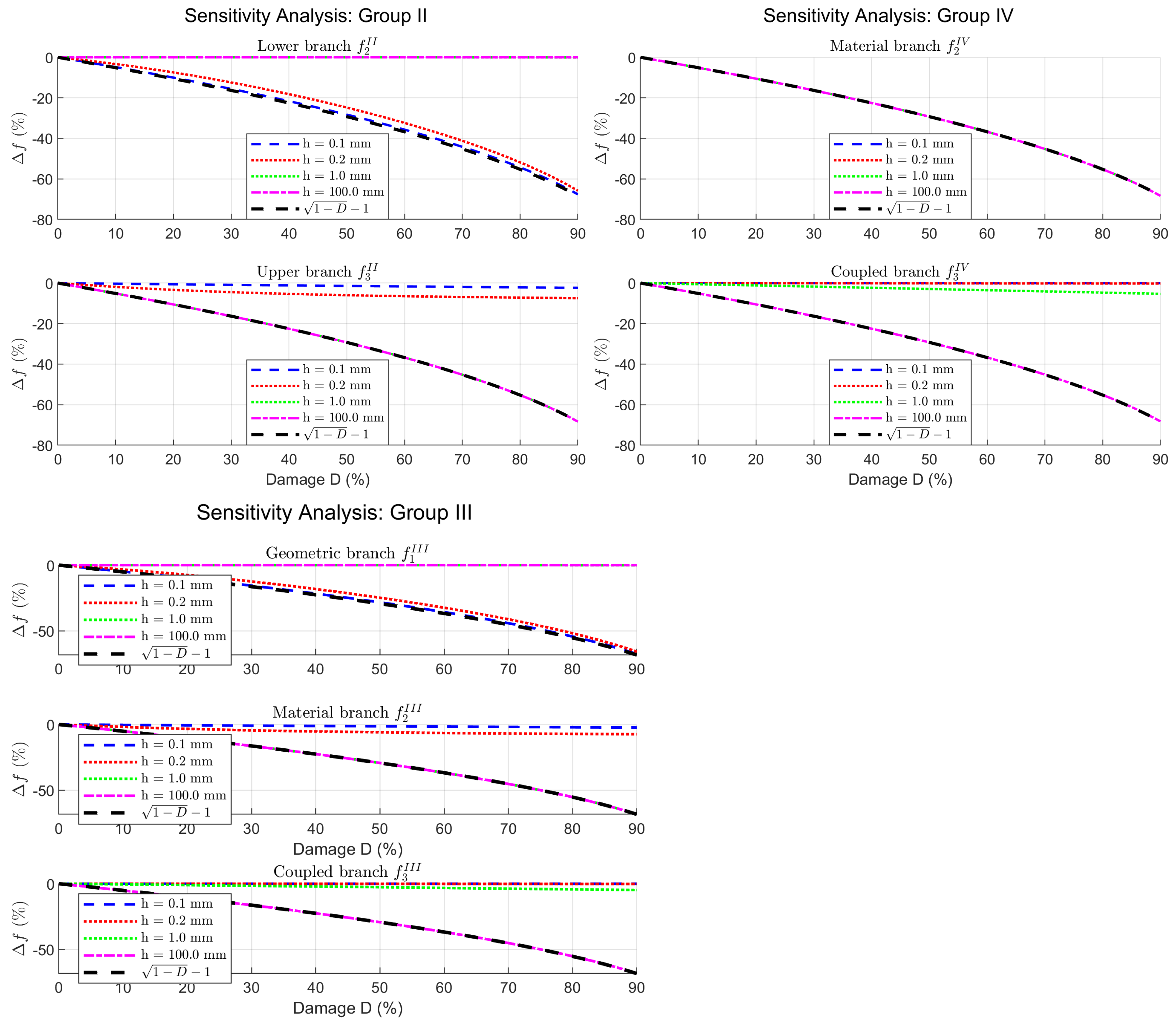

Disclaimer/Publisher’s Note: The statements, opinions and data contained in all publications are solely those of the individual author(s) and contributor(s) and not of MDPI and/or the editor(s). MDPI and/or the editor(s) disclaim responsibility for any injury to people or property resulting from any ideas, methods, instructions or products referred to in the content. |
© 2026 by the author. Licensee MDPI, Basel, Switzerland. This article is an open access article distributed under the terms and conditions of the Creative Commons Attribution (CC BY) license.