


Abstract
Retinal optical coherence tomography (OCT) classification is often affected by substantial class imbalance and by evaluation bias when images from the same patient appear in both training and test sets. This study proposes MCSP-LightP3R-MoE, a patient-aware framework that combines minority-guided cyclic sequential partition learning with progressive lightweight sparse Mixture-of-Experts routing for four-class retinal OCT classification. Group-disjoint training, validation, and test subsets were constructed from 84,484 OCT images covering CNV, DME, DRUSEN, and NORMAL classes. The model uses an ImageNet-pretrained ResNet18 backbone with three progressive LightMoE modules, heterogeneous lightweight experts, and Top-1 routing, and was evaluated over three independent seeds against conventional CNN, imbalance-handling, and ablation baselines. MCSP-LightP3R-MoE achieved 93.28 ± 0.29% balanced accuracy and 92.06 ± 0.37% macro-F1, while DRUSEN sensitivity reached 89.17 ± 1.92%, an 8.78 percentage-point improvement over ResNet18. Patient-cluster bootstrap analysis supported several gains in balanced accuracy and minority-class sensitivity relative to conventional CNN baselines. The model contains 11.57 million parameters, only 3.47% more than ResNet18. These results indicate that patient-aware sequential exposure and sparse expert routing can improve minority-sensitive OCT classification while retaining a single compact inference model.
1. Introduction
Optical coherence tomography (OCT) is a non-invasive imaging modality that provides high-resolution cross-sectional visualization of retinal structures and has become an important tool for the assessment of retinal abnormalities. The rapid growth of OCT imaging has also increased interest in automated image interpretation using deep learning. The study in [1] demonstrated the potential of deep convolutional neural networks for distinguishing clinically relevant retinal conditions from OCT images. Subsequent studies investigated multi-scale convolutional architectures, ensemble strategies, lightweight networks, and hybrid deep learning models to further improve retinal OCT classification [2,3,4,5,6,7]. Recent studies have also demonstrated that advanced image enhancement, representation learning, and feature-fusion strategies can improve medical image segmentation and classification performance [8,9]. These developments have established deep learning as a promising approach for computer-aided retinal image analysis.
Although recent studies have reported high classification performance, class imbalance remains a persistent issue in retinal OCT analysis. In many OCT datasets, the number of images differs considerably across diagnostic categories. As a result, standard training procedures tend to expose the model more frequently to the majority classes, which can bias the learned decision boundaries toward those classes. This means that a model may achieve strong overall accuracy while still performing less reliably on an underrepresented pathological class. In medical image classification, this is particularly important because poor sensitivity for a minority disease class may be clinically more consequential than a small change in overall accuracy.
Class imbalance has been widely studied in machine learning [10]. Common strategies include random over-sampling and under-sampling, synthetic sample generation methods such as SMOTE [11], focal loss [12], and class-balanced loss functions based on the effective number of samples [13]. These approaches can reduce the dominance of majority classes, but they mainly act by changing how often samples are selected or how strongly individual samples contribute to the loss. They do not directly control the way patient groups from different classes are organized and presented to the model during training.
Another important issue is the reliability of the evaluation protocol. Retinal OCT datasets may contain several B-scans from the same patient or acquisition group. If related scans are distributed across both the training and test sets, the reported performance can become overly optimistic because the test data are no longer fully independent of the training data. As shown in [14], such data leakage can substantially inflate classification accuracy in OCT experiments. For this reason, patient-aware data splitting and patient-level uncertainty analysis are important for obtaining a more realistic estimate of model generalization.
From an architectural perspective, residual networks provide a strong basis for medical image classification because they support effective hierarchical feature extraction while remaining considerably more compact than many high-capacity alternatives [15]. However, a conventional convolutional backbone applies essentially the same sequence of feature transformations to every input image. This fixed processing path may be suboptimal when different pathological patterns require different receptive fields or feature transformations.
Mixture-of-Experts (MoE) models provide a mechanism for conditional computation by allowing different inputs to activate different expert branches. Sparse MoE formulations have shown that expert specialization can be introduced without executing every available expert for every input [16]. Top-1 sparse routing further reduces active computation by selecting only the highest-scoring expert for a given representation [17]. Nevertheless, most sparse MoE research has concentrated on large-scale language and general-purpose learning problems. The interaction between sparse expert routing, class imbalance, patient-level data organization, and retinal OCT classification remains comparatively underexplored.
This study addresses these issues from both the data-exposure and feature-processing perspectives. We propose MCSP-LightP3R-MoE, a patient-aware sequential learning framework that combines minority-guided cyclic partition training with progressive sparse expert routing. Rather than repeatedly optimizing the model over the complete imbalanced training distribution, each diagnostic class is decomposed into patient-aware blocks. During a sequential training stage, one block from each class is selected and combined into the current training subset. Blocks belonging to classes with multiple partitions are rotated across stages, whereas minority-class partitions are revisited more frequently. Importantly, majority-class observations are not permanently discarded; they are progressively revisited as the cyclic schedule advances.
The sequential training strategy is coupled with a lightweight ResNet18-based MoE architecture. Three LightMoE modules are introduced at different feature levels of the backbone. Each module contains heterogeneous lightweight experts constructed using different depthwise-convolutional receptive fields. Progressive routing allows deeper routing decisions to incorporate information propagated from earlier stages, while Top-1 selection activates only a single expert within each module for a given input. The resulting framework therefore separates two complementary mechanisms: sequential partitions regulate which training samples are presented to the model, whereas sparse MoE routing regulates which feature transformation is activated for an input.
Unlike ensemble-based approaches, the proposed framework maintains a single continuously optimized network and produces the final prediction using a single inference model. No model averaging or prediction-level ensemble is required. Model selection is performed exclusively on the validation set using macro-F1, while the test set remains isolated until the final checkpoint has been selected. The experimental protocol further employs a reconstructed patient-disjoint training, validation, and test split, multi-seed evaluation, class-specific analysis, calibration measures, and patient-cluster bootstrap uncertainty estimation.
The main contributions of this work are summarized as follows:
- A minority-guided patient-aware sequential partition strategy is proposed for imbalanced retinal OCT classification. The approach increases the effective exposure of underrepresented classes while retaining access to the complete majority-class data through deterministic cyclic block rotation.
- A progressive lightweight sparse mixture-of-experts architecture is introduced on top of ResNet18. Heterogeneous lightweight experts provide different receptive-field transformations, while Top-1 routing activates only one expert at each MoE stage for each input.
- A joint data-exposure and conditional-feature-processing framework is formulated in which sequential partition learning controls the temporal organization of training samples and progressive sparse routing controls feature specialization within the same continuously optimized network.
- A group-disjoint experimental protocol is employed to assess the proposed method against conventional CNN backbones, full imbalanced training, balanced sampling, and targeted architectural and training ablations. Evaluation emphasizes class-balanced performance, minority-class sensitivity, probabilistic calibration, and patient-level statistical uncertainty in addition to conventional overall accuracy.
The remainder of this paper is organized as follows. Section 2 reviews previous work on retinal OCT classification, learning under class imbalance, sparse mixture-of-experts models, sequential learning, and patient-aware evaluation. Section 3 presents the proposed MCSP-LightP3R-MoE framework. Section 4 describes the dataset, group-disjoint split, training configuration, baselines, and evaluation protocol. Section 5 reports the experimental results. Section 6 discusses the main findings and limitations, and Section 7 concludes the study.
2. Related Work
This section reviews the literature most closely related to the proposed framework. The discussion focuses on five aspects: deep learning for retinal OCT classification, learning under class imbalance, sparse mixture-of-experts models, sequential data presentation, and patient-aware evaluation. These directions are closely related to the two main objectives of this study: improving minority-class recognition and maintaining reliable group-disjoint evaluation.
2.1. Deep Learning for Retinal OCT Classification
Deep learning has become a dominant approach for automated retinal OCT analysis. The large-scale study in [1] demonstrated that convolutional neural networks can distinguish several retinal conditions from OCT images with high diagnostic accuracy and helped establish OCT2017 as a widely used benchmark for retinal disease classification.
Subsequent studies explored more sophisticated feature extraction strategies. A multi-scale convolutional neural network ensemble was proposed in [2] to combine complementary representations extracted at different spatial resolutions. Multi-stage and multi-scale ensemble architectures were further investigated in [3], showing that combining information from several feature pathways can improve OCT classification performance.
Other studies focused on reducing model complexity. The approach in [4] investigated an efficient deep learning pipeline for OCT image classification, while a lightweight retinal disease classification model was introduced in [7]. These works demonstrate that competitive OCT classification does not necessarily require very large models.
More recent studies have also investigated transformer-based and hybrid architectures. An interpretable transformer-based network for retinal disease classification was studied in [5], whereas a hybrid convolutional–transformer architecture was proposed in [6]. Such methods broaden the range of feature representations available for OCT analysis, particularly by combining local convolutional information with more global contextual modeling.
Despite these advances, most existing OCT classification methods primarily optimize aggregate classification performance. Less attention has been given to the interaction between model architecture, minority-class recognition, and the temporal organization of imbalanced training data.
2.2. Learning Under Class Imbalance
Class imbalance is a well-established challenge in supervised learning. As discussed in [10], conventional empirical risk minimization can become biased toward majority classes because they contribute disproportionately to the optimization objective.
Several families of solutions have been developed. Data-level approaches modify the training distribution through over-sampling or under-sampling. SMOTE [11], for example, increases minority-class representation by generating synthetic observations in feature space.
Loss-level approaches instead modify the contribution of individual training samples. Focal loss [12] reduces the influence of easily classified observations and emphasizes harder examples, whereas class-balanced loss [13] reweights classes according to the effective number of samples.
These strategies have proven useful across many imbalanced classification tasks. However, they mainly operate at the level of individual samples or loss weights. They do not explicitly organize the training process into complementary class-specific patient partitions or control how those partitions are presented sequentially to a single model.
The proposed MCSP strategy addresses this issue from a different perspective. Rather than modifying only the probability or weight of individual observations, it modifies the temporal structure of data exposure by presenting patient-aware class partitions in a controlled sequence.
2.3. Sparse Mixture-of-Experts and Conditional Feature Processing
Mixture-of-Experts models provide a mechanism for conditional computation by allowing different inputs to activate different processing branches. The sparsely gated MoE formulation introduced in [16] demonstrated that large expert sets can be combined with sparse routing so that only a small subset of experts is evaluated for a given input.
This principle was further simplified in Switch Transformers [17], where Top-1 routing assigns each representation to a single expert. Such sparse routing separates total model capacity from active computation, since the network may store multiple experts while evaluating only one expert per routing decision.
Most classical MoE studies have focused on large-scale language modeling and general-purpose learning. Nevertheless, the underlying idea is also relevant to medical imaging. Pathological image patterns may require different receptive fields or feature transformations, making conditional feature processing potentially useful for heterogeneous retinal structures.
The proposed LightP3R-MoE adopts this principle in a compact convolutional setting. Instead of using large fully connected expert networks, it employs lightweight depthwise-convolutional experts with different receptive-field configurations. Moreover, routing is performed progressively across multiple feature levels rather than independently at a single network stage.
Thus, the proposed model differs from conventional dense multi-branch architectures in that only one expert is activated at each MoE stage for each input.
2.4. Sequential Data Presentation and Partition-Based Training
The order in which training samples are presented can influence the optimization trajectory of a neural network. Curriculum learning [18] established the broader principle that structured data presentation may affect convergence and generalization by controlling the sequence of examples encountered during training.
However, the proposed method is not a conventional curriculum-learning scheme. Samples are not ordered from “easy” to “difficult”, and no difficulty score is assigned to individual OCT images. Instead, the training set is decomposed into class-specific patient-aware blocks, and these blocks are presented according to a deterministic cyclic schedule.
The distinction is important. Curriculum learning primarily changes the order of samples according to estimated difficulty, whereas the proposed approach changes the class composition and patient composition of successive optimization stages.
For class c, the training subset is divided into
and stage-specific training data are constructed from one block per class. The same network is then updated continuously across these stages.
This sequential formulation is intended to reduce persistent majority-class dominance while avoiding permanent removal of majority observations. To the best of our knowledge, the combination of patient-aware class partitioning, deterministic cyclic data exposure, and sparse progressive expert routing has not been systematically investigated for four-class retinal OCT classification.
2.5. Patient-Level Separation and Reliable OCT Evaluation
Reliable evaluation is particularly important in retinal OCT studies because a single patient may contribute multiple highly related B-scans. If images from the same patient or acquisition group occur in both training and test sets, the classifier may exploit subject-specific or acquisition-specific patterns rather than generalizable disease characteristics.
The study in [14] showed that data leakage can substantially inflate reported OCT classification performance. This finding highlights the importance of performing dataset separation at the patient or acquisition-group level rather than randomly splitting individual images.
The present study therefore reconstructs the OCT data split using patient/group identifiers and enforces zero overlap among the training, validation, and test subsets. The same principle is followed in the statistical analysis: uncertainty is estimated using patient-cluster bootstrap resampling rather than treating every B-scan as an independent observation.
This evaluation strategy is intended to provide a more conservative estimate of generalization performance and to reduce the risk that improvements are caused by correlated observations across data subsets.
2.6. Research Gap and Positioning of the Proposed Method
The reviewed literature reveals several complementary developments. Deep CNNs, transformers, and hybrid architectures have substantially improved OCT classification [1,2,5,6]. Imbalance-aware methods modify sampling or loss functions to reduce majority-class bias [10,12,13]. Sparse MoE models provide conditional computation and expert specialization [16,17], while patient-aware evaluation has been shown to be essential for obtaining reliable OCT performance estimates [14].
However, these directions are usually considered separately.
Existing imbalance-handling approaches generally do not explicitly control the sequential exposure of patient groups. Sparse MoE methods generally do not address patient-level class imbalance in retinal OCT data. Conversely, OCT classification studies that employ powerful CNN, transformer, or ensemble architectures typically focus on architectural improvements rather than on coordinating class-balanced data exposure with conditional expert specialization.
The proposed MCSP-LightP3R-MoE framework is positioned at the intersection of these problems. It combines patient-aware sequential partitioning with progressive sparse expert routing while retaining a single continuously optimized model.
The intended contribution is therefore not a new backbone in isolation and not another conventional re-sampling technique. Rather, the method jointly addresses which patient groups are presented during training and which feature transformation is activated for each input. This joint formulation distinguishes the proposed approach from conventional balanced sampling, dense multi-branch architectures, and standard full-data training.
3. Proposed Method
This section presents the proposed MCSP-LightP3R-MoE framework for imbalanced retinal OCT classification. The method combines two complementary mechanisms. The first, termed Minority-Guided Cyclic Sequential Partitioning (MCSP), controls how patient-aware class-specific subsets are exposed to the model during training. The second, LightP3R-MoE, introduces progressive sparse expert routing at multiple feature levels of a ResNet18 backbone.
The central idea is to separate two sources of adaptation. MCSP determines which training samples are presented at a given optimization stage, whereas sparse routing determines which feature transformation is activated for a given input. Both mechanisms operate within a single continuously optimized model; no parameter averaging, model ensemble, or prediction fusion across independently trained networks is required.
3.1. Problem Formulation
Let the retinal OCT training dataset be represented as
where denotes an OCT image, is the corresponding diagnostic label, denotes the patient or acquisition-group identifier associated with the image, and N denotes the total number of images in the dataset.
The classification problem contains four diagnostic categories,
and therefore
For class c, the corresponding subset is
with cardinality
The degree of class imbalance can be expressed by
Under standard empirical risk minimization, the parameters of a classifier are obtained by minimizing
where denotes the classification loss.
Equation (5) can be rewritten in class-wise form as
The factor
shows that larger classes naturally contribute more frequently to the total optimization objective. Consequently, strong overall accuracy may coexist with weaker sensitivity for an underrepresented category.
The objective of the proposed method is therefore to learn a single classifier
that maintains competitive overall discrimination while reducing class-dependent performance imbalance.
3.2. Overview of MCSP-LightP3R-MoE
The complete framework consists of two interacting components:
- MCSP training, which partitions each diagnostic class into patient-aware blocks and presents complementary block combinations according to a deterministic cyclic schedule;
- LightP3R-MoE, which introduces three progressive lightweight Mixture-of-Experts modules into a ResNet18 backbone and performs Top-1 sparse expert selection.
The interaction between these two components can be summarized as
and
Thus, the proposed framework addresses class imbalance at the training-data level while simultaneously allowing input-dependent feature specialization inside the network.
Figure 1 illustrates the overall architecture.
Figure 1.
Overall architecture of the proposed MCSP-LightP3R-MoE framework. Patient-aware class blocks are sequentially combined by MCSP, while three progressive LightMoE modules perform sparse Top-1 conditional feature processing within the ResNet18 backbone.
3.3. Patient-Aware Class Partition Construction
MCSP is constructed exclusively from the training subset. Let denote the training images belonging to class c.
Given a target block size B, the number of blocks assigned to class c is defined as
The class-specific training set is then partitioned into
The partition satisfies
and
Importantly, partitioning is performed at the patient/group level rather than at the individual-image level. All images associated with a given patient identifier are assigned to the same class-specific block.
Let
denote the patient groups belonging to class c, where each group contains all images sharing the same patient/group identifier.
The patient groups are ordered according to their number of images, and each group is assigned to the currently smallest block:
The complete patient group is then added as
This greedy patient-aware allocation seeks to keep block sizes approximately balanced while preventing any patient/group from being divided across multiple blocks.
Unlike conventional random undersampling, the proposed strategy does not permanently discard observations from large classes. Majority-class images that are absent from one stage remain available through other blocks and are presented in subsequent stages.
3.4. Minority-Guided Cyclic Sequential Scheduling
After constructing the class-specific blocks, the maximum number of blocks is defined as
A complete MCSP cycle therefore contains sequential optimization stages.
At cycle r and stage s, the selected block index for class c is determined using deterministic cyclic rotation:
The stage-specific training subset is then constructed as
Equation (16) ensures that classes containing multiple blocks are progressively rotated through the sequential stages.
For a minority class with the index remains for every stage. Consequently, the minority block is revisited more frequently, whereas majority-class blocks are rotated.
This mechanism increases the effective exposure of the minority class without permanently reducing the available information from higher-frequency classes.
The schedule is deterministic at the block level. However, after constructing , samples are randomly shuffled before mini-batches are generated. Thus, the proposed procedure combines deterministic stage composition with stochastic mini-batch optimization.
The previously reported shuffled-order ablation only modifies the presentation order of preconstructed MCSP stages; it retains the class-specific blocks and their stage composition. It is therefore not an exposure-matched, non-partitioned control. We separately introduce such a control in Section 4.4 to distinguish the effects of class-exposure frequency from those of block-structured sequencing.
3.5. Continuous Sequential Optimization
A defining characteristic of MCSP is that all sequential stages update the same model.
Let denote the parameter state at cycle r and stage s.
After training on the stage-specific subset , the model is updated as
where denotes the gradient-based optimization procedure.
The model is not reinitialized when the stage changes. Likewise, parameters from independently trained blocks are not averaged. Instead, optimization follows one continuous parameter trajectory:
This formulation distinguishes the proposed method from ensemble learning, federated averaging, and independently trained partition models.
The same AdamW optimizer instance, including its running first- and second-moment states, is retained across all five stages of a cycle and across consecutive cycles. Neither model parameters nor optimizer states are reset at a stage boundary. Learning-rate scheduling is indexed by the cumulative optimizer-update count rather than by the local stage or nominal full-data epoch. We use a linear warmup over the first 5% of the planned updates, followed by cosine decay to 5% of the initial learning rate. The global schedule is not restarted at stage or cycle boundaries.
After every complete cycle, the current model is evaluated on the validation set. If denotes validation macro-F1 after cycle r, the selected cycle is
The final checkpoint is therefore
The test set is not involved in partition construction, sequential scheduling, hyperparameter adjustment, or checkpoint selection.
3.6. LightP3R-MoE Architecture
The feature-processing component of the proposed framework is built on an ImageNet-pretrained ResNet18 backbone [15].
Three feature levels are used for conditional expert processing:
The first two feature maps correspond to relatively shallow residual representations, while the third represents the deeper semantic feature level.
A lightweight Mixture-of-Experts module is associated with each level:
After the final feature stage, global average pooling and a four-class linear classifier generate the prediction.
The complete classification mapping can be written conceptually as
3.7. Heterogeneous Lightweight Experts
Each LightMoE module contains four lightweight experts:
where denotes the feature level.
Rather than using full convolutional branches, each expert follows a bottleneck depthwise-convolution structure:
The channel-reduction factor is
Thus, if the input channel dimension is , the intermediate representation contains approximately channels.
The four experts use different spatial transformations:
where d denotes the dilation factor.
This design provides expert branches with different effective receptive fields while keeping each branch computationally lightweight.
The heterogeneous expert set is intended to provide alternative feature transformations for OCT patterns occurring at different spatial scales.
3.8. Progressive Top-1 Sparse Routing
For each feature level, global average pooling is first applied:
A routing network then produces expert logits
which are converted into routing probabilities using softmax:
The first routing stage depends only on the corresponding pooled feature representation. Since produces routing logits, the routing probabilities are obtained by applying the softmax function:
The second router incorporates both the current pooled representation and the routing probabilities from the first stage:
The third router additionally incorporates the probability representations from both preceding routing stages:
Here, denotes feature concatenation. Importantly, the routing probability vectors and are passed to subsequent routers without applying a stop-gradient or detach operation.
Consequently, the computational graph connecting the progressive routing stages is preserved, allowing gradients from subsequent stages to propagate to earlier routing networks.
For every stage, only the highest-probability expert is activated:
To enable classification-driven optimization of the routing networks while preserving hard Top-1 expert activation, a straight-through-style selected-probability surrogate is introduced.
The selected expert output is defined as
Here, denotes the stop-gradient operator, which preserves its input value during the forward pass but blocks its derivative during backpropagation.
Residual fusion is then performed as
Therefore, although four experts are stored within each module, only one expert branch is active for a given input at each feature level.
This differs from dense multi-branch feature fusion, in which all branches are evaluated and subsequently combined.
During the forward pass, the straight-through surrogate satisfies
because the stop-gradient operator returns the same numerical value as its input.
Therefore, the forward computation reduces to
which is identical to conventional hard Top-1 expert activation.
During backpropagation, however, the stop-gradient operator has zero derivative. Hence,
The softmax derivative is
where denotes the indicator function.
Consequently, the classification objective provides a differentiable surrogate path from the selected expert output through the routing probabilities to the router logits and parameters.
The discrete expert-selection index itself remains non-differentiable and is treated as fixed during backpropagation.
Only the selected expert is evaluated for each input, whereas the softmax probability representation allows classification gradients to update the routing network.
In addition, since the probability vectors from earlier routing stages are not detached, gradients from deeper routers can propagate through the progressive routing connections.
The auxiliary load-balancing objective provides an additional gradient signal for the router parameters, independently of the classification-driven surrogate gradient.
3.9. Joint Classification and Load-Balancing Objective
The primary classification objective is label-smoothed cross-entropy.
For a sample with target label y, the smoothed target distribution is defined as
where denotes the smoothing coefficient.
The classification loss is
where denotes the mini-batch size and is the predicted probability of class c.
Sparse routing can potentially collapse toward a small subset of experts. To discourage this behavior, a load-balancing term is introduced.
For expert k at MoE stage l, the mean routing probability within a mini-batch is
For four experts, the uniform routing target is
The stage-specific load-balancing objective penalizes deviations in the mean soft routing probabilities from the uniform target and is defined as
The total routing regularization is
The final training objective is
with
The load-balancing objective regularizes the mean soft routing probabilities, rather than the actual frequency of hard Top-1 expert assignments.
Consequently, approximately uniform average routing probabilities do not necessarily imply that all experts are selected equally often.
To distinguish these two quantities, the empirical hard assignment proportion of expert k at MoE stage l is defined as
where N denotes the number of processed image presentations and is the indicator function.
Unlike the mean soft routing probability , the quantity directly measures the fraction of inputs assigned to each expert.
The hard assignment proportions are analyzed separately for all three MoE stages and four diagnostic classes throughout training.
3.10. Interaction Between Sequential Partitioning and Sparse Experts
The two major components of the proposed framework address different aspects of the learning process.
For a sequential stage, determines which patient-aware class blocks contribute to the current optimization updates.
Within the model, the routing function determines which expert transformation is activated for image x at feature level l.
Thus,
whereas
This separation is important because the proposed method does not rely solely on architectural capacity or solely on rebalancing the data distribution. Instead, it combines controlled exposure to imbalanced classes with conditional feature transformations.
Algorithm 1 highlights three important properties of the proposed training procedure. First, patient-aware blocks are constructed exclusively from the training data. Second, the same network is updated continuously across all sequential stages and cycles. Third, validation macro-F1 is used for checkpoint selection, while the test set remains completely isolated until final evaluation.
| Algorithm 1 MCSP-LightP3R-MoE Training Procedure |
|
3.11. Computational Characteristics of Top-1 Routing
The proposed architecture stores multiple experts but activates only one expert at each LightMoE stage for a given input.
If denotes the computational cost of expert k at stage l, dense evaluation of all experts would require approximately
In contrast, Top-1 routing activates only the selected expert:
The approximate inference cost of the full model can therefore be expressed as
This distinction between stored parameters and active computation is particularly important for sparse MoE architectures. Although all expert branches contribute to the total parameter count, they are not all evaluated for every OCT image.
Measured inference efficiency is evaluated in Section 5.9. These measurements complement the theoretical complexity analysis but do not constitute a complete clinical deployment assessment.
4. Experimental Setup
This section describes the dataset, group-disjoint data split, preprocessing pipeline, sequential partition configuration, comparison models, optimization settings, evaluation metrics, and statistical analysis used to assess the proposed MCSP-LightP3R-MoE framework.
4.1. Dataset and Group-Disjoint Split
The experiments were conducted on the retinal OCT dataset introduced in [1]. The complete collection used in this study contained 84,484 OCT B-scans from four diagnostic categories: CNV, DME, DRUSEN, and NORMAL. The class distribution comprised 37,455 CNV, 11,598 DME, 8866 DRUSEN, and 26,565 NORMAL images, corresponding to a largest-to-smallest class-imbalance ratio of approximately 4.22:1.
The original directory-level split was not used directly for the final evaluation. Previous work has shown that multiple retinal OCT B-scans may originate from the same patient or acquisition group, and image-level separation may therefore lead to optimistic performance estimates [14]. According to the original OCT2017 dataset documentation [19], filenames follow the convention CLASS-ID-IMAGE, where ID denotes a randomized patient identifier and IMAGE represents the corresponding image number.
In our implementation, the extracted identifier was used as a global grouping key across all four diagnostic classes. The diagnostic class label was not included in the grouping key. The complete collection of 84,484 images contained 4657 distinct global identifiers, of which 896 occurred in more than one diagnostic class.
Importantly, identifiers shared across different classes were not treated as independent groups. Instead, all images associated with the same identifier were assigned to the same data subset.
Although the original dataset documentation describes these identifiers as randomized patient IDs, independent verification of the underlying clinical identities was not available. Therefore, the term group-disjoint is used consistently to describe the experimental partitioning protocol.
The group-disjoint split was generated with target image proportions of 70%, 10%, and 20% for training, validation, and testing, respectively. For each global identifier, the numbers of CNV, DME, DRUSEN, and NORMAL images were first determined. Each complete group was then assigned to exactly one subset using a deterministic group-level optimization procedure. The algorithm employed rarity-weighted greedy initialization, up to four passes of local reassignment, and 32 optimization restarts with split seed 2026. The selected partition minimized deviations from the target class-specific image counts and group proportions without dividing individual groups. The resulting subsets contained 59,140 training images, 8449 validation images, and 16,895 test images. These correspond to actual proportions of 70.0014%, 10.0007%, and 19.9979%, respectively. The class-specific distributions are reported in Table 1, whereas the global group statistics are presented in Table 2.
Table 1.
Group-disjoint OCT dataset split used in the experiments.
Table 2.
Group-level partition statistics of the OCT2017 dataset.
Let , , and denote the sets of distinct global group identifiers in the training, validation, and test subsets, respectively.
The group-disjoint partitioning procedure enforces the following non-overlap conditions:
The actual identifier-overlap audit confirmed that
Thus, no global group identifier was shared between any two data subsets.
Furthermore, the 896 identifiers appearing across multiple diagnostic classes were counted only once in the global group inventory.
All images associated with each such identifier remained within the same subset.
The group counts reported in Table 2 therefore correspond to unique global identifiers rather than class-wise identifier totals.
The split was generated once and then fixed for all baseline, ablation, and proposed-model experiments. Sequential partitions were constructed exclusively from the training subset, the validation subset was used for checkpoint selection, and the test subset remained isolated until final evaluation.
4.2. Image Preprocessing and Data Augmentation
All OCT images were converted to three-channel format and resized to pixels before being supplied to the network. During training, lightweight geometric augmentation was applied to reduce sensitivity to small acquisition-related variations while avoiding aggressive transformations that could alter diagnostically relevant retinal morphology. The training pipeline included random horizontal flipping and small affine perturbations, whereas validation and test images were processed deterministically without stochastic augmentation.
All images were normalized using the ImageNet channel statistics and . The same validation and test preprocessing pipeline was used for all compared models.
4.3. Patient-Aware Sequential Block Configuration
The sequential partitions were generated only from the fixed training subset containing 59,140 images. The target block size was set to approximately 5000 images. Application of the partition rule in Equation (8) produced five CNV blocks, two DME blocks, one DRUSEN block, and four NORMAL blocks; hence, , and each complete MCSP cycle contained five sequential training stages.
The resulting patient-aware block sizes are summarized in Table 3.
Table 3.
Patient-aware class blocks used for sequential MCSP training.
Because DRUSEN contains only one block, the same DRUSEN partition is revisited across the five sequential stages, whereas blocks from the higher-frequency categories are cyclically rotated. This mechanism increases effective exposure of the minority category without permanently discarding majority-class observations.
Observed Exposure Frequency
The block configuration yields unequal nominal presentation frequencies per complete cycle: approximately one pass for CNV, 2.5 passes for DME, five passes for DRUSEN, and 1.25 passes for NORMAL. Over ten cycles, the nominal class presentations are 262,180, 202,975, 310,350, and 232,450, respectively. Mini-batch formation with drop_last=True reduces the realized counts; across the three training seeds, the model performs 1,005,760 actual image presentations rather than the 1,007,955 nominal presentations. We therefore report observed, not only theoretical, exposure counts in Table 4. An exposure denotes one image presentation during optimization, not a distinct image.
Table 4.
Actual class-wise MCSP training exposure over ten cycles. Counts are means ± standard deviations across seeds 17, 29, and 43. The exposure-matched random-mixing control reproduces the exact counts for each class, seed, and cycle.
4.4. Baseline and Ablation Configurations
The experimental comparison was organized into three groups: conventional CNN baselines, imbalance-handling strategies, and targeted ablation variants. The conventional CNN baselines included ResNet18, MobileNetV3-Small, EfficientNet-B0, and DenseNet121. ResNet18 [15] served as the direct backbone reference because the proposed architecture is built on this network, while DenseNet121 [20], EfficientNet-B0 [21], and MobileNetV3-Small [22] provided additional strong and efficient CNN comparisons.
For imbalance-related comparisons, the same LightP3R-MoE architecture was evaluated using direct full-data training (LightP3R-FullImbalanced) and conventional balanced sampling (LightP3R-BalancedSampler). The ablation experiments further compared Top-1 and Top-2 sparse routing, deterministic cyclic and shuffled sequential scheduling, progressive and independent routing, and heterogeneous and homogeneous expert configurations.
4.4.1. Exposure-MatchedRandom-Mixing Control
To control for exposure frequency, we also trained the corrected hard Top-1 straight-through MoE with a globally mixed, non-block training stream (MoE-ST Random Mixing). For each seed and each of the ten cycles, the numbers of CNV, DME, DRUSEN, and NORMAL presentations were copied exactly from that seed’s realized MCSP exposure log. Images were sampled with replacement within each class and then globally shuffled; MCSP stage blocks and their deterministic order were not used. The same fixed group-disjoint split, model configuration, optimizer-update budget (15,715), and ten validation/checkpoint opportunities were used. Because within-class sampling was with replacement, the design matches class-level presentation counts, not the per-image multiplicities of the MCSP stream. This distinction limits causal attribution of any differences exclusively to the ordering of individual samples.
4.4.2. New Controlled Component and Loss Baselines
Rationale for a separate controlled experiment. Following the reconstruction of the dataset partition at the global identifier level (Section 4.1), we established one fixed group-disjoint training/validation/test split containing 59,140/8,449/16,895 images. The additional component and loss baselines, together with a newly trained corrected Top-1 ST reference, were evaluated as a separate matched-budget experiment on this same revised split. These runs were not obtained by extending the original experimental configurations summarized in Table 5 or the original routing ablation experiments. The earlier tables document the original experimental configurations and routing ablations; their results must not be pooled with the new matched-budget comparisons as though all runs used the same revised partition and corrected routing implementation. The new controls and their corrected reference were therefore evaluated and compared within the same matched-budget protocol.
Table 5.
Baseline and ablation configurations. These are the original experimental configurations; the additional controls were evaluated separately under a matched-budget protocol using the reconstructed fixed group-disjoint split.
To separate the MCSP presentation schedule from the contribution of progressive sparse experts, we added ResNet18+MCSP, using the same MCSP stage stream but omitting all MoE modules. As loss-level controls, we trained ResNet18 with standard cross-entropy (CE), inverse-frequency-weighted CE, focal loss (focusing exponent ), and effective-number-based class-balanced CE (). Class weights were calculated from the training split alone; the weighted-loss controls did not use MCSP staging. The focal objective was applied to the per-example CE term, with the same label-smoothing setting () as the other controls. For architectural context, we additionally include a corrected Top-1 ST MoE trained with the standard full-data stream, without MCSP.
These additional controls share the same fixed group-disjoint split, initialization protocol, random seeds, optimizer-update budget, validation schedule, and checkpoint-selection criterion. Except for the ResNet18+MCSP component-isolation control, class-wise presentation frequencies need not match the MCSP schedule. Consequently, the loss baselines test alternative strategies under matched total training budgets, not under identical class exposures.
The original experimental configurations are summarized in Table 5, whereas the additional controlled baselines form a separate matched-budget comparison.
All configurations within the additional matched-budget experiment used the same fixed group-disjoint data split and test evaluation protocol. Model selection was performed exclusively using validation macro-F1.
4.5. Implementation and Training Configuration
The proposed MCSP-LightP3R-MoE framework and all comparison models were implemented in Python 3.12 using PyTorch 2.5.1 and Torchvision 0.20.1 (CUDA 12.1).
ImageNet-pretrained weights were used for the convolutional backbones where applicable, and all models used the same input preprocessing protocol.
The proposed model was optimized using AdamW [23] with an initial learning rate of , weight decay of , and a mini-batch size of 64. Label-smoothed cross-entropy [24] was used with , while the load-balancing coefficient was fixed at . Each LightMoE module contained four heterogeneous experts with a channel-reduction factor of , and the final configuration used Top-1 sparse routing.
For MCSP training, the target block size was approximately 5000 images, with five sequential stages per cycle. One local epoch was performed at each stage, and training was limited to 10 cycles, corresponding to at most 50 sequential stages. The same network parameters were carried continuously from one stage to the next; the model was not reinitialized between partitions or cycles.
After each complete cycle, the current checkpoint was evaluated on the validation set, and the model with the highest validation macro-F1 was retained for final evaluation. The test set was not used for checkpoint selection, hyperparameter adjustment, or any other model-selection decision. To assess stochastic training variability, the principal experiments were independently repeated using random seeds 17, 29, and 43 while keeping the group-disjoint data split fixed.
To verify gradient propagation through the proposed hard Top-1 routing mechanism, the model was retrained using the straight-through-style surrogate with three independent random seeds (17, 29, and 43).
For each seed, classification-only router gradients were examined at the beginning of each of the ten MCSP training cycles.
Importantly, the auxiliary load-balancing loss was excluded from these diagnostic gradient calculations, allowing the classification-driven gradient pathway to be examined independently.
Across the resulting 30 diagnostic evaluations, all three MoE routers exhibited finite, nonzero classification gradient norms, corresponding to 90 nonzero router gradient measurements.
The minimum observed gradient norms were , , and for the first, second, and third MoE routers, respectively.
These observations confirm that the implemented surrogate enables classification-loss gradients to reach all three progressive routing modules at the examined training points.
The main architectural and optimization settings are summarized in Table 6.
Table 6.
Main implementation and training configuration.
4.5.1. Matched Training-Budget Protocol
A single MCSP cycle comprises five sequential stages and is therefore not equivalent to one conventional full-data epoch. The training split contains 59,140 images. An MCSP cycle nominally presents approximately 100,796 images, whereas a conventional complete pass through the training split would present 59,140 images. Because incomplete stage-specific mini-batches are discarded, the realized MCSP exposure is 1,005,760 image presentations across ten cycles (100,576 per cycle on average), corresponding to 15,715 optimizer updates with batch size 64. The resulting exposure budget is approximately 17.01 complete full-data passes, not ten conventional epochs.
For an optimization-budget-controlled comparison, the corrected MCSP-LightP3R-MoE (Top-1 ST) reference and the eight newly trained controls were evaluated with exactly the same total optimizer updates, image-presentation budget, and validation/checkpoint-selection opportunities (Table 7). For all three seeds (17, 29, 43), validation took place after cumulative updates 1572, 3143, 4715, 6286, 7857, 9428, 11,000, 12,571, 14,143, and 15,715. Each method consequently offered ten checkpoints for selection by the same validation macro-F1 criterion. The common AdamW optimization schedule used an initial learning rate of , weight decay , a 5% global linear warmup, and subsequent cosine decay; its progress was measured in optimizer updates rather than epochs. Optimizer states persisted throughout the training of each individual run, including across MCSP stages.
Table 7.
Realized training budgets for the corrected Top-1 ST reference and the new matched-budget controls. Counts are per seed; all three seeds (17, 29, 43) gave identical totals. Each validation check is also a checkpoint-selection opportunity.
These controls match the total number of processed image presentations, but do not generally match class-wise exposure frequencies: standard full-data training, balanced sampling, and MCSP use different sampling strategies. Only the separate exposure-matched random-mixing control also matches the number of presentations for each diagnostic class in each cycle and seed (Section 4.4). This matched-budget analysis applies to the newly trained controls in Table 7; it should not be taken to retroactively establish equal budgets for earlier experiments outside this controlled comparison.
4.5.2. Computational Environment
All experiments were conducted on a workstation running Windows 11, equipped with an Intel Core i9-12900K processor, 128 GB of RAM, and an NVIDIA GeForce RTX 4090 GPU with 24 GB of video memory. The same computational environment was used for the conventional baselines, imbalance-handling methods, ablation experiments, and the proposed MCSP-LightP3R-MoE configuration.
4.6. Evaluation Metrics
Standard classification measures included overall accuracy, class-wise precision, sensitivity, specificity, F1-score, and multiclass Matthews correlation coefficient (MCC). Because the dataset is imbalanced, balanced accuracy and macro-F1 were treated as principal aggregate metrics. They were computed as
and
One-vs-rest receiver operating characteristic and precision–recall analyses were used to obtain class-specific and macro-averaged AUROC and AUPRC values. Since DRUSEN was the smallest diagnostic category, dedicated DRUSEN precision, sensitivity, specificity, F1-score, AUROC, and AUPRC were also reported.
4.7. Calibration Evaluation
In addition to discrimination performance, probabilistic calibration was evaluated using negative log-likelihood (NLL), Brier score, and expected calibration error (ECE), following established neural-network calibration analysis [25]. NLL was computed as
the multiclass Brier score as
and ECE as
Lower values indicate better calibration for all three measures.
4.8. Statistical Analysis Methodology
Statistical uncertainty was assessed using bootstrap resampling [26], adapted to the patient-clustered structure of the test data. Pairwise comparisons between MCSP-LightP3R-MoE and the principal baseline models were performed using 5000 paired patient-cluster bootstrap replicates. Resampling was conducted at the patient/group level rather than at the individual-image level so that all OCT images associated with a sampled identifier remained together.
For metric q, the paired difference between the proposed model and a comparator was calculated as
and the 95% percentile confidence interval was obtained as
where denotes the -quantile of the bootstrap distribution. Hierarchical resampling was additionally used to combine patient-level sampling uncertainty with variability across the three training seeds. The principal comparisons focused on balanced accuracy, macro-F1, DRUSEN sensitivity, and DRUSEN F1, with overall accuracy included as a complementary metric. A difference was interpreted as statistically supported when the corresponding 95% confidence interval did not include zero.
Paired Hierarchical Group–Seed Bootstrap Procedure
Within each experimental series, the proposed and comparator models use the same held-out images and group identifiers for each training seed (17, 29, and 43). Before resampling, predictions are paired by normalized image path, global group identifier, and true class label. The paired differences therefore use an identical sampled test population for both models; predictions are never resampled independently.
For the reconstructed-split matched-budget series, each seed has 931 test-group identifiers. These are sampled with replacement 5000 times, drawing 931 groups per replicate. Every image belonging to a sampled group remains together. If a group is drawn more than once, all of its images contribute with the same multiplicity to both models’ confusion matrices. For each replicate, we aggregate the resulting group-level confusion counts into one four-class confusion matrix per model and calculate accuracy, balanced accuracy, macro-F1, DRUSEN sensitivity, and DRUSEN F1 from these aggregate counts. The paired metric difference is then computed within that seed.
To incorporate training-seed variability, a second resampling level draws three seed indices with replacement from the three available seeds. For each selected seed, one of its previously generated group-bootstrap replicates is drawn, and the three paired metric differences are averaged with equal weight. This yields 5000 hierarchical replicates, whose 2.5th and 97.5th percentiles define the reported 95% confidence interval. The point estimate is the unweighted mean of the three observed seed-specific differences, rather than a metric recomputed from predictions pooled across seeds. The corresponding two-sided bootstrap p-value is estimated from the proportions of hierarchical replicates on either side of zero; for the new matched-budget comparison family, these values were additionally checked using Holm correction across 40 method–metric tests.
Importantly, this procedure quantifies conditional test-group and training-seed variability for one fixed group-disjoint split. It does not sample alternative train/validation/test partitions, and thus does not measure split-to-split, external-dataset, or acquisition-domain variability. Group identifiers follow the dataset naming convention; independently validated patient linkage is unavailable. With only three training seeds, conclusions from hierarchical intervals must also remain cautious.
4.9. Reproducibility Protocol
To reduce experimental bias, the following protocol was maintained throughout the study:
- the group-disjoint training, validation, and test split was generated once and reused across all experiments;
- sequential blocks were constructed exclusively from the training subset;
- validation macro-F1 was used for checkpoint selection;
- the test subset was not used for hyperparameter selection or early stopping;
- identical test samples were used for all competing methods;
- the principal experiments were repeated with random seeds 17, 29, and 43;
- results were reported as mean ± standard deviation across the three runs;
- patient-cluster bootstrap analysis was used to quantify test-set uncertainty.
This protocol separates model selection, training variability, and test-population uncertainty and provides a common evaluation basis for the proposed model, the conventional CNN baselines, and the imbalance-handling alternatives.
5. Results
This section evaluates the proposed MCSP-LightP3R-MoE framework from several complementary perspectives. First, its overall classification performance is compared with conventional CNN backbones. The analysis is then extended to class-wise behavior, with particular attention to the underrepresented DRUSEN category. Next, the proposed sequential partition strategy is compared with conventional imbalance-handling approaches, followed by an ablation analysis. Finally, statistical uncertainty, training stability, calibration, and model complexity are examined.
Unless otherwise stated, the reported values represent the mean and standard deviation over three independent runs using random seeds 17, 29, and 43.
5.1. Comparison with Conventional CNN Baselines
The first experiment compares the proposed framework with commonly used convolutional architectures under the same group-disjoint evaluation protocol. Since overall accuracy may conceal weaknesses in lower-frequency classes, both aggregate and class-balanced metrics are considered.
Table 8 summarizes the results.
Table 8.
Comparison with conventional CNN baselines on the group-disjoint test set. Values are reported as mean ± standard deviation over three independent runs.
The results reveal a clear distinction between overall accuracy and class-balanced performance. DenseNet121 and EfficientNet-B0 achieved slightly higher raw accuracy, whereas MCSP-LightP3R-MoE obtained the highest balanced accuracy. Relative to its direct ResNet18 backbone, the proposed framework increased balanced accuracy by 1.69 percentage points while maintaining a comparable overall accuracy.
The macro-F1 score also remained close to those of the strongest conventional baselines. These findings indicate that the main effect of MCSP-LightP3R-MoE is not simply to increase the total number of correct predictions, but to distribute classification performance more evenly across the four diagnostic categories.
Figure 2 illustrates this difference.
Figure 2.
Balanced accuracy of the proposed method and the principal comparison models. Error bars indicate the standard deviation across three independent runs.
The proposed configuration also showed relatively low variability across the three independent runs. However, Table 8 confirms that no single model dominates every evaluation criterion. The principal advantage of MCSP-LightP3R-MoE is therefore its stronger class-balanced behavior rather than uniform superiority across all aggregate metrics.
5.2. Class-Wise Performance
To identify which diagnostic categories contribute most strongly to the change in balanced accuracy, class-specific performance was analyzed separately for CNV, DME, DRUSEN, and NORMAL.
Table 9 presents the corresponding results.
Table 9.
Class-wise performance of MCSP-LightP3R-MoE.
NORMAL remained the easiest category to classify, whereas DRUSEN was the most challenging. Nevertheless, the proposed framework substantially improved recognition of the minority class. Relative to ResNet18, DRUSEN sensitivity increased by 8.78 percentage points, while DRUSEN F1 increased by 2.68 percentage points.
The minority-class sensitivity comparison is shown in Figure 3.
Figure 3.
DRUSEN sensitivity across the principal comparison models. Error bars indicate the standard deviation across three independent runs.
The figure shows that conventional balanced sampling already improves DRUSEN recognition substantially, but the final MCSP configuration provides the highest mean sensitivity.
To examine the remaining classification errors in more detail, a representative run was selected as the seed whose macro-F1 was closest to the three-seed mean. Seed 29 satisfied this criterion. Its normalized confusion matrix is shown in Figure 4.
Figure 4.
Row-normalized confusion matrix of MCSP-LightP3R-MoE for the representative run (seed 29).
The confusion matrix confirms strong sensitivity across all four classes. The dominant residual error involves DRUSEN samples being classified as CNV. Approximately 10% of DRUSEN images were assigned to the CNV category in the representative run. This suggests that the main remaining limitation is associated with separation between these two pathological patterns rather than general minority-class under-recognition.
5.3. ROC and Precision–Recall Analysis
Threshold-independent discrimination was assessed using one-vs-rest ROC and precision–recall analyses.
Figure 5 presents the ROC curves for the representative run.
Figure 5.
One-vs-rest ROC curves of MCSP-LightP3R-MoE for the representative run (seed 29). The diagonal dashed line represents the performance of a random classifier (AUC = 0.5).
The AUROC values were 0.984 for CNV, 0.986 for DME, 0.969 for DRUSEN, and 0.998 for NORMAL. These values indicate strong ranking performance across all four diagnostic categories, although DRUSEN remained the most difficult class.
Since ROC analysis may provide an optimistic impression under class imbalance, precision–recall curves were examined separately, as shown in Figure 6.
Figure 6.
One-vs-rest precision–recall curves of MCSP-LightP3R-MoE for the representative run (seed 29).
The average precision values were 0.971 for CNV, 0.935 for DME, 0.893 for DRUSEN, and 0.993 for NORMAL. The larger gap observed for DRUSEN in the precision–recall domain further confirms that this category remains the principal classification challenge.
5.4. Comparison with Imbalance-Handling Strategies
The next experiment investigates whether the minority-class improvement can be reproduced using simpler imbalance-handling methods. For this purpose, the same LightP3R-MoE architecture was trained using the original imbalanced distribution, conventional balanced sampling, and the proposed MCSP strategy.
The results of the imbalance-handling comparison are summarized in Table 10.
Table 10.
Comparison of imbalance-handling strategies using the same LightP3R-MoE architecture.
Direct training on the naturally imbalanced distribution produced the weakest DRUSEN sensitivity and the largest across-seed variation. Balanced sampling substantially reduced this problem and represents a strong comparison method.
MCSP produced a different precision–sensitivity balance. It achieved the highest balanced accuracy and DRUSEN sensitivity, whereas BalancedSampler retained slightly higher overall accuracy, macro-F1, DRUSEN precision, and DRUSEN F1. Thus, the proposed strategy should be interpreted as favoring greater minority-class sensitivity rather than uniformly outperforming conventional balanced sampling.
5.5. Ablation Study
The ablation study evaluates the contributions of routing sparsity, partition ordering, progressive routing, and expert heterogeneity.
The corresponding ablation results are presented in Table 11.
Table 11.
Ablation study of MCSP-LightP3R-MoE: original routing variants from the earlier experimental series, before the Top-1 ST correction and the separate matched-budget experiments on the reconstructed group-disjoint split. The new controlled comparisons were evaluated under a separate matched-budget experimental protocol.
The earlier Top-1/Top-2 and shuffled-order ablations describe the behavior of their respective original configurations. In particular, the shuffled-order experiment reorders preconstructed MCSP stages and does not remove block structure. The new corrected straight-through Top-1 MCSP and its exposure-matched non-block control are evaluated separately in Table 12; unlike the original shuffled-order ablation, this comparison directly tests block-structured scheduling against class-exposure-matched random mixing.
Table 12.
Exposure-matched scheduling control on the fixed group-disjoint test set. Values are mean ± standard deviation across three seeds (%). Both variants use the corrected hard Top-1 ST router.
The earlier NoProgressive and HomogeneousExperts results characterize the original ablation configurations but do not isolate an interaction effect under the corrected Top-1 ST training protocol. The new matched-budget ResNet18+MCSP and loss-controlled experiments provide a more direct test of the architectural and imbalance-handling contributions, as described below.
5.5.1. Exposure-Matched Random-Mixing Control
To separate the contribution of class presentation frequencies from the use of deterministic sequential blocks, the newly retrained MCSP-LightP3R-MoE (Top-1 ST) model was compared with a Top-1 ST MoE trained using global random mixing with precisely matched class-wise presentation counts in every seed and cycle. Each configuration was trained for ten cycles, corresponding to 15,715 optimizer updates and 1,005,760 actual image presentations per seed. The test results from validation-macro-F1-selected checkpoints are reported in Table 12.
Relative to MCSP-ST, random mixing increased mean accuracy by 0.50 percentage points and macro-F1 by 0.44 percentage points, whereas DRUSEN sensitivity decreased by 2.22 percentage points. For the paired group-and-seed bootstrap (5000 replicates), the random-mixing-minus-MCSP-ST difference was percentage points for macro-F1 (95% CI: ) and percentage points for DRUSEN sensitivity (95% CI: ). Both intervals include zero, so the observed trends do not establish statistically significant superiority of either scheduling strategy. The result is consistent with a trade-off between overall macro-F1 and minority-class sensitivity, rather than a general advantage of deterministic block ordering. Moreover, class-level exposure equality does not guarantee identical per-image repetitions. This limitation is explicitly acknowledged when interpreting the scheduling comparison.
5.5.2. Interpretation Under Matched Training Budgets
The comparison above is not driven by differing total optimizer-step budgets or by a greater number of validation checkpoints: both the MCSP-ST reference and its matched random-mixing control used 15,715 updates, 1,005,760 image presentations, and ten validation evaluations per seed. Under these matched conditions, the MCSP-ST reference achieved 91.90% macro-F1 and 88.61% DRUSEN sensitivity, compared with 92.34% and 86.39% for random mixing, respectively. For context, the separately trained step-matched MoE-ST full-data control obtained 92.54% macro-F1 and 83.38% DRUSEN sensitivity. These observations indicate different class-performance trade-offs at a common optimization budget; they do not demonstrate that the MCSP schedule is uniformly superior or that total sample exposures being matched also equalizes class-specific sampling frequencies.
5.5.3. Component Isolation and Loss-Based Controls
Because the global-ID-based group-disjoint dataset split was reconstructed, we performed this component-and-loss comparison as a separate controlled experiment, rather than inserting incomparable results into the original configuration and ablation tables. Both the corrected MCSP-LightP3R-MoE (Top-1 ST) reference and every new baseline were trained on the same fixed revised split. The requested ResNet18+MCSP control and three complementary imbalance-aware losses were evaluated under the same training budget as that corrected ST reference. The ResNet18+MCSP control retained the sequential class-block stream but removed all three sparse MoE modules, thereby isolating the architectural change under MCSP. The other ResNet18 baselines used standard full-data mixing and alternative loss functions. Results for three seeds and validation-selected test checkpoints are summarized in Table 13.
Table 13.
Separate matched-budget component and imbalance-loss experiment on the reconstructed fixed group-disjoint OCT2017 split; results are not pooled with the original configuration and routing ablation tables. All methods use 15,715 updates and ten validation opportunities per seed. Results are means ± standard deviations over seeds 17, 29 and 43 (%). Class-wise exposures are not identical across all methods.
The full MCSP-ST model obtained 93.83% accuracy, 91.90% macro-F1, and 88.61% DRUSEN sensitivity. Removing its MoE modules while retaining MCSP increased accuracy to 94.31% and macro-F1 to 92.36%, but lowered DRUSEN sensitivity to 86.22%. Thus, the additional architecture does not improve aggregate test metrics in this comparison; rather, it shifts the observed class-wise trade-off.
Among the loss-based ResNet18 controls, focal loss achieved the highest mean accuracy (94.86%) and macro-F1 (92.87%), but its DRUSEN sensitivity was 82.89%, compared with 88.61% for MCSP-ST. Inverse-frequency-weighted CE produced 86.37% DRUSEN sensitivity, while effective-number-based class-balanced CE produced 84.11%. For comparison, the full-data ST-MoE control obtained 83.38% DRUSEN sensitivity. These results do not support a claim of uniform superiority of the combined MCSP–MoE architecture.
Using paired group-and-seed bootstrap resampling (5000 replicates), the ResNet18+MCSP-minus-MCSP-ST DRUSEN-sensitivity difference was percentage points (95% CI: ; Holm-adjusted over the 40 tested comparisons). The corresponding macro-F1 difference was percentage points (95% CI: ), which includes zero. For focal loss, the macro-F1 difference was percentage points (nominal 95% CI: ), but its Holm-adjusted p-value did not establish significance. Its DRUSEN-sensitivity difference was percentage points (95% CI: ), indicating lower sensitivity than MCSP-ST.
These paired intervals characterize performance on this fixed train/validation/test split with three training seeds; they do not account for variation arising from independent data splits or external datasets. The results identify a minority-sensitivity trade-off, not a demonstrated positive interaction or causal synergy between MCSP and the MoE modules. The underlying factorial interaction would require further matched component controls.
To assess the effectiveness of the soft load-balancing objective, we recorded actual hard Top-1 expert assignments for all three MoE stages throughout the ten MCSP training cycles.
The analysis was conducted independently for random seeds 17, 29, and 43. For each stage and cycle, the fraction of image presentations assigned to each of the four experts was computed.
Figure 7 illustrates the resulting assignment trajectories.
Figure 7.
Hard Top-1 expert assignment proportions across ten MCSP training cycles for three random seeds and three progressive MoE stages. Each curve represents one expert. The dotted horizontal line indicates uniform assignment at 25%. The results reveal seed- and stage-dependent deviations from balanced expert utilization.
The results reveal that approximately balanced expert utilization during early training does not guarantee balanced assignments in later cycles.
In particular, for seed 29 at the third MoE stage during cycle 10, the four experts received 0, 31,286, 69,321, and 1 assignments, respectively, out of 100,608 image presentations.
Similarly, for seed 43, the second expert at the third MoE stage received only five assignments during cycle 10.
These findings indicate substantial expert underutilization in some training configurations despite the presence of soft probability regularization.
Class-conditional assignment statistics were also examined to assess whether the routing mechanism exhibited diagnosis-dependent expert preferences.
For seed 29 at the third MoE stage during cycle 10, DRUSEN images were predominantly assigned to Expert 2 (98.35%), whereas CNV, DME, and NORMAL images were predominantly assigned to Expert 3 (98.86%, 99.89%, and 97.87%, respectively).
These observations indicate that the routing mechanism can exhibit class-dependent assignment patterns.
However, the strong concentration of multiple classes on a single expert, together with substantial variations across training seeds, prevents interpreting these patterns as conclusive evidence of balanced or consistently reproducible expert specialization.
The assignment statistics describe routing behavior during training; they do not independently establish the causal contribution of individual experts to classification performance.
5.5.4. Effect of Load-Balancing Regularization
To isolate the effect of the soft load-balancing regularizer, we compared the original setting () with an additional ablation in which the coefficient was set to zero. The two configurations used the same group-disjoint data split, random seeds (17, 29, and 43), Top-1 straight-through routing mechanism, and training budget (15,715 optimizer updates per seed). Test metrics were computed from the checkpoint selected using validation macro-F1 in each seed. Table 14 reports the resulting three-seed classification performance.
Table 14.
No-balancing ablation: test-set classification performance (mean ± standard deviation across three random seeds, in %).
Removing the balancing term produced small changes in predictive performance: mean accuracy increased from 93.81% to 94.09% and macro-F1 from 91.85% to 92.12%, whereas DRUSEN sensitivity remained nearly unchanged (87.89% versus 87.87%). The balanced configuration retained slightly higher macro-AUROC and macro-AUPRC. These descriptive three-seed results do not establish a consistent predictive advantage for either setting.
To assess the role of balancing in routing behavior, we further compared the hard Top-1 assignments at the third MoE stage. Table 15 distinguishes assignment statistics at the validation-selected cycle from those at the final (cycle 10) training stage. This distinction is important because the final training cycle is not necessarily the checkpoint selected for testing.
Table 15.
Third-stage hard Top-1 expert utilization with and without load balancing (mean across three seeds). Selected-cycle statistics refer to the validation-selected cycle; final-cycle statistics refer to training cycle 10.
The balancing term was associated with more diverse hard expert assignments, particularly at the third MoE stage. The mean final-cycle normalized entropy was 0.7245 with balancing, compared with 0.2717 without balancing, while the mean dominant-expert assignment share increased from 49.41% to 82.74% when the balancing term was removed.
In the no-balancing run with seed 43, every image presentation at MoE-3 during cycle 10 was assigned to a single expert, indicating complete hard-routing collapse at that point in training. Nevertheless, the regularized model also exhibited unequal hard assignments in some configurations; balancing did not eliminate expert underutilization in every seed.
Together with the class-specific assignment analysis and Figure 7, these results support interpreting the soft balancing term as a routing-utilization regularizer rather than a guarantee of uniformly distributed hard assignments or improved classification accuracy. With only three seeds, these utilization differences are descriptive and should not be presented as statistically established superiority.
5.6. Statistical Analysis
Paired patient-cluster bootstrap analysis with 5000 replicates was used to determine whether the observed performance differences were robust to patient-level variation. Hierarchical resampling additionally incorporated variability across the three independent training seeds.
Positive differences in Table 16 favor MCSP-LightP3R-MoE.
Table 16.
Hierarchical patient-cluster bootstrap comparison of MCSP-LightP3R-MoE with selected baselines. Differences are reported in percentage points. Original series.
Table 16 belongs to the original experimental series and is retained to document the initial paired comparisons. Its three LightP3R-BalancedSampler confidence intervals all include zero; therefore, the initial comparisons do not establish MCSP’s statistical superiority over that sampling baseline. The corrected Top-1 ST comparison on the reconstructed group-disjoint split is reported separately in Table 17.
Table 17.
New controlled series. Fixed-split matched-budget Top-1 ST comparison with MoE-ST BalancedSampler; paired hierarchical 95% confidence intervals from 5000 replicates across three seeds. Differences are MCSP-ST minus BalancedSampler, in percentage points.
The bootstrap analysis provides the strongest evidence against the direct ResNet18 backbone. The confidence intervals for balanced accuracy, DRUSEN sensitivity, and DRUSEN F1 remain entirely above zero. Against DenseNet121, the improvements in balanced accuracy and DRUSEN sensitivity are also supported, whereas the DRUSEN F1 difference is not conclusive.
For EfficientNet-B0, the balanced-accuracy interval crosses zero, but the improvement in DRUSEN sensitivity remains positive. The comparison with BalancedSampler is more conservative: although MCSP produced higher mean balanced accuracy and sensitivity, the corresponding intervals included zero. Therefore, the evidence supports improved minority recognition relative to conventional CNN training, but not uniform statistical superiority over balanced sampling.
Separate Corrected Top-1 ST Comparison with Balanced Sampling
Following the reconstructed fixed group-disjoint split and Top-1 ST routing correction, both MCSP-ST and the MoE-ST BalancedSampler control were evaluated using the same three training seeds and matched training budgets. Table 17 reports the new paired hierarchical-bootstrap results. To maintain the positive-is-better convention used in the original statistical table, the differences below are presented as ; the computational output was consistently sign-reversed from its comparator-minus-reference convention, including the interval bounds.
All five confidence intervals in the new balanced-sampling comparison include zero, consistent with the limitation already recognized in the original Table 16. MCSP-ST obtained a numerically higher mean DRUSEN sensitivity (88.61% versus 86.52%), but the paired difference of +2.09 percentage points (95% CI: ) does not establish a statistically supported advantage over BalancedSampler. The new results therefore support a qualified, class-sensitive trade-off, not a claim of uniform or statistically demonstrated superiority to balanced sampling. The confidence intervals remain conditional on the one fixed split and the three training seeds.
5.7. Training Stability
The sequential optimization process does not necessarily produce monotonic improvements after every cycle. Figure 8 illustrates the validation macro-F1 trajectory for the representative run.
Figure 8.
Validation macro-F1 across sequential MCSP cycles for the representative run (seed 29).
Moderate fluctuations are observed across cycles, confirming the importance of validation-based checkpoint selection rather than automatically retaining the final training state.
Across the three independent runs, macro-F1 was , while balanced accuracy was . The relatively small standard deviations indicate that the main class-balanced behavior was reproducible across the evaluated initializations.
5.8. Calibration Performance
The proposed model achieved an expected calibration error (ECE) of , a Brier score of , and a negative log-likelihood (NLL) of . These values characterize the confidence quality of the final MCSP-LightP3R-MoE model under the group-disjoint test protocol. Since the present comparison tables focus on discrimination and class-balanced metrics, the calibration results are reported as descriptive properties of the proposed model rather than as evidence of uniform superiority over the baseline architectures.
5.9. Model Complexity
The final MCSP-LightP3R-MoE model contained 11,566,384 trainable parameters, compared with 11,178,564 parameters for the standard ResNet18 backbone. The expert and routing modules therefore introduced 387,820 additional parameters, corresponding to an increase of approximately 3.47%.
Importantly, the total stored parameter count does not correspond directly to active inference computation. Under Top-1 routing, only one expert is evaluated at each LightMoE stage for a given OCT image.
Measured GPU Inference Efficiency
To complement the parameter-count comparison, we measured single-image GPU inference performance for ResNet18 and the corrected MCSP-LightP3R-MoE (Top-1 ST) model.
Measurements were performed on an NVIDIA RTX 4090 GPU using FP32 precision, input images, and batch size 1, with 100 warm-up iterations followed by 500 measured forward passes.
The measured GPU inference efficiency results, including parameter counts, computational complexity, inference latency, and throughput, are summarized in Table 18.
Table 18.
GPU inference efficiency of ResNet18 and MCSP-LightP3R-MoE (Top-1 ST). FLOPs are approximate THOP-based estimates; FPS is derived from mean forward-pass latency.
The proposed architecture increased the number of trainable parameters by approximately 3.47% and the estimated FLOPs by 0.66% relative to ResNet18.
However, mean GPU inference latency increased from 1.164 ms to 3.181 ms per image, representing an approximately 2.73-fold increase.
This difference may reflect the execution overhead associated with dynamic expert selection and sparse routing, although the underlying causes were not separately verified through operation-level profiling.
The FLOP values are approximate estimates and may not account for all custom routing operations. Moreover, the reported FPS values exclude image preprocessing, data transfer, and clinical workflow overhead.
Therefore, the measurements characterize GPU inference efficiency under the evaluated conditions but do not independently establish real-time clinical readiness.
6. Discussion
Under the new matched-budget controls, MCSP-LightP3R-MoE (Top-1 ST) attained the highest mean DRUSEN sensitivity, whereas ResNet18+MCSP and several standard or imbalance-aware loss baselines obtained higher mean overall accuracy or macro-F1. Differences in balanced accuracy were smaller. Accordingly, the findings are interpreted as a class-sensitive trade-off under the fixed group-disjoint split, rather than evidence of uniform superiority across metrics or a proven synergistic interaction of MCSP and MoE.
6.1. Effect of Sequential Partition Learning
MCSP changes the class composition of optimization updates by constructing group-safe blocks and presenting one block from each class at every stage. This increases repeated exposure of DRUSEN samples. However, the exposure-matched random-mixing experiment shows that the contribution of deterministic block order cannot be isolated as a significant improvement in overall performance. Its mean DRUSEN sensitivity was higher than random mixing, but the paired confidence interval included zero. Thus, the observed minority-sensitive pattern may reflect increased class exposure and/or the optimization trajectory; it cannot be attributed solely to the sequential order of blocks.
Unlike conventional undersampling, majority-class observations are not permanently discarded. Instead, different majority-class blocks are revisited as the cyclic schedule progresses. At the same time, classes with fewer partitions are encountered more frequently across sequential stages. This provides increased exposure to the minority class while preserving access to the complete training data over the full optimization trajectory.
The comparison with BalancedSampler is particularly informative. Balanced sampling achieved slightly higher macro-F1 and DRUSEN F1, whereas MCSP produced higher balanced accuracy and DRUSEN sensitivity. Therefore, the proposed strategy should not be interpreted as a uniformly superior replacement for balanced sampling. Rather, the two methods produce different operating points: conventional balanced sampling provides a somewhat more precision-oriented solution, while MCSP favors greater minority-class sensitivity.
Crucially, all three original balanced-sampling intervals in Table 16, and all five updated fixed-split ST intervals in Table 17, span zero. Consequently, the observed DRUSEN-sensitivity advantage is a numerical tendency rather than evidence of statistically established added value over balanced sampling. This qualification is retained when discussing the role of MCSP scheduling and sparse routing.
Clinical Implications of the Sensitivity–Precision Trade-Off
The clinical relevance of the observed trade-off between minority-class sensitivity, precision, and overall classification performance depends on the intended application and the relative consequences of diagnostic errors.
In screening-oriented workflows, higher DRUSEN sensitivity may help reduce missed pathological cases and support timely referral for further clinical evaluation. However, improved sensitivity should be considered alongside precision and false-positive rates, since unnecessary referrals may increase the workload of ophthalmologists and the burden of additional examinations.
In contrast, diagnostic decision-support systems may require a more balanced consideration of false-negative and false-positive errors, with operating thresholds selected according to clinical priorities and the intended workflow.
Importantly, the present experiments do not quantify the clinical costs of these errors or establish an optimal decision threshold.
Furthermore, the observed differences between MCSP and balanced sampling do not establish statistically significant superiority.
Therefore, the proposed framework should be regarded as an experimentally evaluated classification approach rather than a clinically validated diagnostic system.
Future work should investigate threshold-dependent performance, clinical decision costs, external validation on independent patient cohorts, and prospective assessment within realistic ophthalmological workflows.
6.2. Role of Sparse Expert Routing
The second component of the proposed framework is progressive sparse expert routing. The ablation experiments showed that Top-1 routing was sufficient to achieve competitive performance and that activating a second expert did not provide a consistent advantage. This finding supports the use of sparse routing because only one expert is evaluated at each LightMoE stage for a given input.
The expert modules provide alternative receptive-field transformations, and progressive routing permits deeper decisions to incorporate earlier routing information. However, the new ResNet18+MCSP control achieved higher mean accuracy and macro-F1 than the corrected MCSP-ST model, while the latter showed higher DRUSEN sensitivity. Therefore, these experiments do not establish a synergistic gain in overall classification from combining MCSP with sparse experts. They instead reveal different performance trade-offs under the shared sequential training protocol. The original NoProgressive and HomogeneousExperts ablations remain descriptive architectural comparisons and should not be interpreted as a controlled interaction test for the corrected ST implementation.
The previous shuffled-order ablation varied the ordering of preconstructed MCSP stages, while the new matched random-mixing control removed the block structure at the same per-class presentation budget. These are distinct controls. The matched comparison produced numerically higher macro-F1 for random mixing and higher DRUSEN sensitivity for MCSP-ST, without confidence intervals excluding zero for these two metrics. Accordingly, stage ordering is regarded as a design choice with potentially different class-specific effects, not as a demonstrated source of uniform performance gains.
6.3. Reliability, Limitations, and Future Work
The group-disjoint evaluation protocol is an important aspect of the present study. Multiple OCT B-scans may originate from the same patient or acquisition group, and leakage between training and test subsets can lead to optimistic performance estimates [14]. By enforcing patient/group separation and using patient-cluster bootstrap analysis, the experimental protocol provides a more conservative assessment of model generalization.
Despite the improvement in DRUSEN sensitivity, the confusion-matrix and precision–recall analyses show that DRUSEN remains the most difficult category. The dominant residual error involves confusion between DRUSEN and CNV, suggesting that further improvement may require more discriminative pathology-specific representations rather than additional rebalancing alone.
Several limitations should also be acknowledged. Because the present study uses a reconstructed patient/group-disjoint split, its numerical results should not be directly compared with studies evaluated using the original image-level OCT2017 directory split. First, the experiments were conducted on a single public OCT dataset containing four diagnostic categories. External validation on independently collected datasets and images acquired using different devices is therefore required to assess cross-domain generalization. Second, patient grouping was derived from the identifiers available in the dataset naming structure and should ideally be confirmed using clinical metadata when such information is available. Third, the principal experiments were repeated using three random seeds; although the observed variability was relatively small, a larger number of independent runs would provide stronger evidence regarding training stability.
Moreover, the reported group–seed bootstrap intervals are conditional on the single reconstructed train/validation/test partition. They do not incorporate uncertainty from constructing another group-disjoint split, and the limited number of training seeds constrains inference about optimization variability. Additional independently constructed splits and external cohorts are required before generalizing the reported confidence intervals beyond this evaluation protocol.
Finally, the measured GPU inference results indicate that the proposed architecture introduces a modest increase in estimated FLOPs but substantially greater single-image latency than ResNet18.
Although the observed latency is relatively low under the evaluated GPU configuration, real-world deployment performance also depends on preprocessing, data transfer, hardware availability, and clinical workflow requirements.
Future work will therefore include end-to-end latency evaluation, external OCT validation, and prospective assessment under realistic clinical conditions.
Overall, the findings suggest that patient-aware sequential partition learning and sparse Top-1 expert routing provide complementary mechanisms for improving minority-sensitive retinal OCT classification while retaining a single compact inference model.
7. Conclusions
This study presented MCSP-LightP3R-MoE, a patient-aware sequential learning framework for imbalanced retinal OCT classification. The method combines minority-guided cyclic partition training with progressive sparse Top-1 expert routing in a single ResNet18-based model. By controlling both the temporal exposure of class-specific patient groups and the conditional transformation of intermediate features, the framework was designed to improve class-balanced recognition without relying on model ensembles.
In the corrected matched-budget evaluation, the proposed framework achieved 88.61% mean DRUSEN sensitivity, compared with 86.22% for ResNet18+MCSP without MoE and 82.89% for a ResNet18 focal-loss baseline, while showing lower mean accuracy and macro-F1 than these controls. The group-and-seed paired bootstrap indicated a DRUSEN-sensitivity difference of percentage points relative to ResNet18+MCSP (Holm-adjusted ), on the fixed data split. These results support a class-sensitive operating-point interpretation, not a general performance gain from combining the components.
The results also revealed an important trade-off. Some conventional baselines and balanced sampling achieved slightly higher overall accuracy, macro-F1, or DRUSEN precision. Therefore, the contribution of the proposed method is not uniform superiority across all metrics, but a shift toward more balanced classification and stronger recognition of the underrepresented pathological class.
Overall, the findings demonstrate that patient-aware sequential partition learning and sparse conditional expert processing can be effectively integrated within a single compact inference model for retinal OCT classification. Future work will focus on external validation across independent OCT datasets, adaptive partition scheduling, improved discrimination between DRUSEN and CNV, and a more detailed evaluation of inference efficiency in terms of FLOPs, latency, throughput, and memory consumption.
Author Contributions
Conceptualization, O.Y. and K.S.; methodology, O.Y. and K.S.; software, K.S. and Y.K.; validation, O.T., K.S. and S.K.; formal analysis, O.Y. and O.T.; investigation, O.Y., O.T., K.S. and Y.K.; data curation, S.K. and Y.K.; writing—original draft preparation, O.Y.; writing—review and editing, O.Y., K.S., O.T., Y.K. and S.K.; visualization, S.K. and K.S.; supervision, O.Y.; project administration, O.Y. and O.T.; funding acquisition, O.Y. All authors have read and agreed to the published version of the manuscript.
Funding
This research was supported by the Agency for Innovative Development under the Ministry of Higher Education, Science and Innovation of the Republic of Uzbekistan, project No. AL-9224104661.
Institutional Review Board Statement
Not applicable. This study used only a publicly available, de-identified retinal OCT dataset and involved no new collection of human participant data.
Informed Consent Statement
Not applicable.
Data Availability Statement
The retinal OCT dataset analyzed in this study is publicly available as described in [1]. No new clinical data were collected or generated in this study.
Acknowledgments
During the preparation of this manuscript, the authors used GPT-5.6 (OpenAI) solely for Uzbek-language translation, grammatical correction, linguistic editing, and improvements in text clarity and readability. The manuscript was independently written by the authors. All research ideas, scientific contributions, methodologies, algorithms, experiments, data analyses, results, and conclusions were developed and obtained through the authors’ own research and practical experimental work, without AI-generated scientific content. All content was carefully reviewed and verified by the authors, who take full responsibility for the accuracy, originality, scientific integrity, and final version of the manuscript.
Conflicts of Interest
The authors declare no conflicts of interest.
Abbreviations
The following abbreviations are used in this manuscript:
| OCT | Optical coherence tomography |
| CNV | Choroidal neovascularization |
| DME | Diabetic macular edema |
| MCSP | Minority-Guided Cyclic Sequential Partitioning |
| MoE | Mixture-of-Experts |
| CNN | Convolutional neural network |
| GAP | Global average pooling |
| AUROC | Area under the receiver operating characteristic curve |
| AUPRC | Area under the precision–recall curve |
| MCC | Matthews correlation coefficient |
| ECE | Expected calibration error |
| NLL | Negative log-likelihood |
References
- Kermany, D.S.; Goldbaum, M.; Cai, W.; Valentim, C.C.S.; Liang, H.; Baxter, S.L.; McKeown, A.; Yang, G.; Wu, X.; Yan, F.; et al. Identifying Medical Diagnoses and Treatable Diseases by Image-Based Deep Learning. Cell 2018, 172, 1122–1131.e9. [Google Scholar] [CrossRef] [Scilit] [PubMed]
- Rasti, R.; Rabbani, H.; Mehridehnavi, A.; Hajizadeh, F. Macular OCT Classification Using a Multi-Scale Convolutional Neural Network Ensemble. IEEE Trans. Med. Imaging 2018, 37, 1024–1034. [Google Scholar] [CrossRef] [Scilit] [PubMed]
- Akinniyi, O.; Rahman, M.M.; Sandhu, H.S.; El-Baz, A.; Khalifa, F. Multi-Stage Classification of Retinal OCT Using Multi-Scale Ensemble Deep Architecture. Bioengineering 2023, 10, 823. [Google Scholar] [CrossRef] [Scilit] [PubMed]
- Kian Ara, R.; Matiolański, A.; Dziech, A.; Baran, R.; Domin, P.; Wieczorkiewicz, A. Fast and Efficient Method for Optical Coherence Tomography Images Classification Using Deep Learning Approach. Sensors 2022, 22, 4675. [Google Scholar] [CrossRef] [Scilit] [PubMed]
- He, J.; Wang, J.; Han, Z.; Ma, J.; Wang, C.; Qi, M. An Interpretable Transformer Network for the Retinal Disease Classification Using Optical Coherence Tomography. Sci. Rep. 2023, 13, 3637. [Google Scholar] [CrossRef] [Scilit] [PubMed]
- Laouarem, A.; Kara-Mohamed, C.; Bourennane, E.-B.; Hamdi-Cherif, A. HTC-Retina: A Hybrid Retinal Diseases Classification Model Using Transformer-Convolutional Neural Network from Optical Coherence Tomography Images. Comput. Biol. Med. 2024, 178, 108726. [Google Scholar] [CrossRef] [Scilit] [PubMed]
- Pan, H.; Miao, J.; Yu, J.; Dong, J.; Zhang, M.; Wang, X.; Feng, J. A Lightweight Model for the Retinal Disease Classification Using Optical Coherence Tomography. Biomed. Signal Process. Control 2025, 101, 107146. [Google Scholar] [CrossRef] [Scilit]
- Abduvaitov, A.; Buriboev, A.S.; Sultanov, D.; Buriboev, S.; Yusupov, O.; Jasur, K.; Choi, A.J. Enhancing Medical Image Segmentation and Classification Using a Fuzzy-Driven Method. Sensors 2025, 25, 5931. [Google Scholar] [CrossRef] [Scilit] [PubMed]
- Buriboev, A.S.; Oh, R.; Nishanov, A.; Dusonov, K.; Narzullaev, I.; Buribayev, S.; Yusupov, O.; Abduvaytov, A.; Axmedova, A.; Lee, C.; et al. Classification and Segmentation of Medical Images Using Cross-Representation Attention Fusion and Fuzzy Image Enhancement. Sensors 2026, 26, 4364. [Google Scholar] [CrossRef] [Scilit] [PubMed]
- He, H.; Garcia, E.A. Learning from Imbalanced Data. IEEE Trans. Knowl. Data Eng. 2009, 21, 1263–1284. [Google Scholar] [CrossRef] [Scilit]
- Chawla, N.V.; Bowyer, K.W.; Hall, L.O.; Kegelmeyer, W.P. SMOTE: Synthetic Minority Over-Sampling Technique. J. Artif. Intell. Res. 2002, 16, 321–357. [Google Scholar] [CrossRef] [Scilit]
- Lin, T.-Y.; Goyal, P.; Girshick, R.; He, K.; Dollár, P. Focal Loss for Dense Object Detection. In Proceedings of the IEEE International Conference on Computer Vision (ICCV), Venice, Italy, 22–29 October 2017; pp. 2980–2988. [Google Scholar] [CrossRef] [Scilit]
- Cui, Y.; Jia, M.; Lin, T.-Y.; Song, Y.; Belongie, S. Class-Balanced Loss Based on Effective Number of Samples. In Proceedings of the IEEE/CVF Conference on Computer Vision and Pattern Recognition (CVPR), Long Beach, CA, USA, 15–20 June 2019; pp. 9268–9277. [Google Scholar] [CrossRef] [Scilit]
- Tampu, I.E.; Eklund, A.; Haj-Hosseini, N. Inflation of Test Accuracy Due to Data Leakage in Deep Learning-Based Classification of OCT Images. Sci. Data 2022, 9, 580. [Google Scholar] [CrossRef] [Scilit] [PubMed]
- He, K.; Zhang, X.; Ren, S.; Sun, J. Deep Residual Learning for Image Recognition. In Proceedings of the IEEE Conference on Computer Vision and Pattern Recognition (CVPR), Las Vegas, NV, USA, 27–30 June 2016; pp. 770–778. [Google Scholar] [CrossRef] [Scilit]
- Shazeer, N.; Mirhoseini, A.; Maziarz, K.; Davis, A.; Le, Q.; Hinton, G.; Dean, J. Outrageously Large Neural Networks: The Sparsely-Gated Mixture-of-Experts Layer. In Proceedings of the International Conference on Learning Representations (ICLR), Toulon, France, 24–26 April 2017. [Google Scholar]
- Fedus, W.; Zoph, B.; Shazeer, N. Switch Transformers: Scaling to Trillion Parameter Models with Simple and Efficient Sparsity. J. Mach. Learn. Res. 2022, 23, 120. [Google Scholar]
- Bengio, Y.; Louradour, J.; Collobert, R.; Weston, J. Curriculum Learning. In Proceedings of the 26th Annual International Conference on Machine Learning (ICML), Montreal, QC, Canada, 14–18 June 2009; pp. 41–48. [Google Scholar] [CrossRef] [Scilit]
- Kermany, D.; Zhang, K.; Goldbaum, M. Labeled Optical Coherence Tomography (OCT) and Chest X-Ray Images for Classification. In Mendeley Data; Elsevier: Amsterdam, The Netherlands, 2018; Version 2. [Google Scholar] [CrossRef]
- Huang, G.; Liu, Z.; van der Maaten, L.; Weinberger, K.Q. Densely Connected Convolutional Networks. In Proceedings of the IEEE Conference on Computer Vision and Pattern Recognition (CVPR), Honolulu, HI, USA, 21–26 July 2017; pp. 2261–2269. [Google Scholar] [CrossRef] [Scilit]
- Tan, M.; Le, Q.V. EfficientNet: Rethinking Model Scaling for Convolutional Neural Networks. In Proceedings of the 36th International Conference on Machine Learning (ICML), Long Beach, CA, USA, 9–15 June 2019; PMLR: Cambridge, MA, USA, 2019; Volume 97, pp. 6105–6114. [Google Scholar]
- Howard, A.; Sandler, M.; Chu, G.; Chen, L.-C.; Chen, B.; Tan, M.; Wang, W.; Zhu, Y.; Pang, R.; Vasudevan, V.; et al. Searching for MobileNetV3. In Proceedings of the IEEE/CVF International Conference on Computer Vision (ICCV), Seoul, Republic of Korea, 27 October–2 November 2019; pp. 1314–1324. [Google Scholar] [CrossRef] [Scilit]
- Loshchilov, I.; Hutter, F. Decoupled Weight Decay Regularization. In Proceedings of the International Conference on Learning Representations (ICLR), New Orleans, LA, USA, 6–9 May 2019. [Google Scholar]
- Szegedy, C.; Vanhoucke, V.; Ioffe, S.; Shlens, J.; Wojna, Z. Rethinking the Inception Architecture for Computer Vision. In Proceedings of the IEEE Conference on Computer Vision and Pattern Recognition (CVPR), Las Vegas, NV, USA, 27–30 June 2016; pp. 2818–2826. [Google Scholar] [CrossRef] [Scilit]
- Guo, C.; Pleiss, G.; Sun, Y.; Weinberger, K.Q. On Calibration of Modern Neural Networks. In Proceedings of the 34th International Conference on Machine Learning (ICML), Sydney, Australia, 6–11 August 2017; PMLR: Cambridge, MA, USA, 2017; Volume 70, pp. 1321–1330. [Google Scholar]
- Efron, B.; Tibshirani, R.J. An Introduction to the Bootstrap; Chapman & Hall: New York, NY, USA, 1993. [Google Scholar]
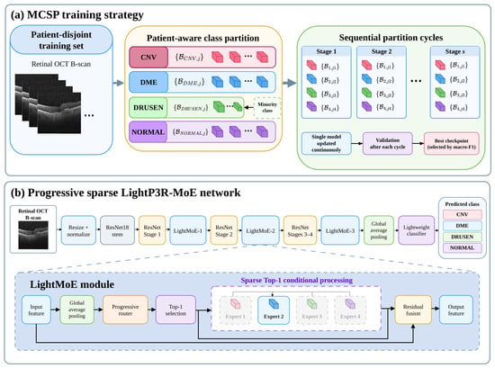
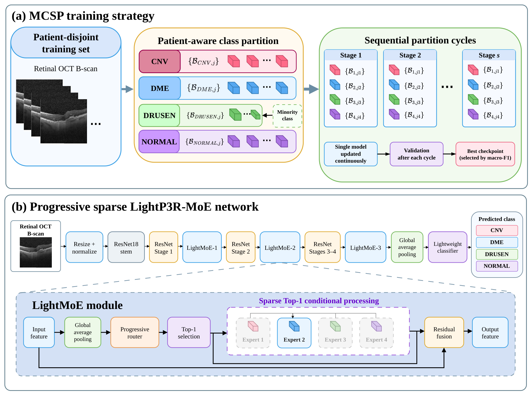
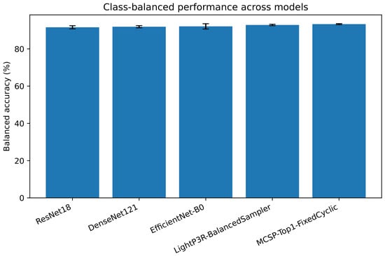
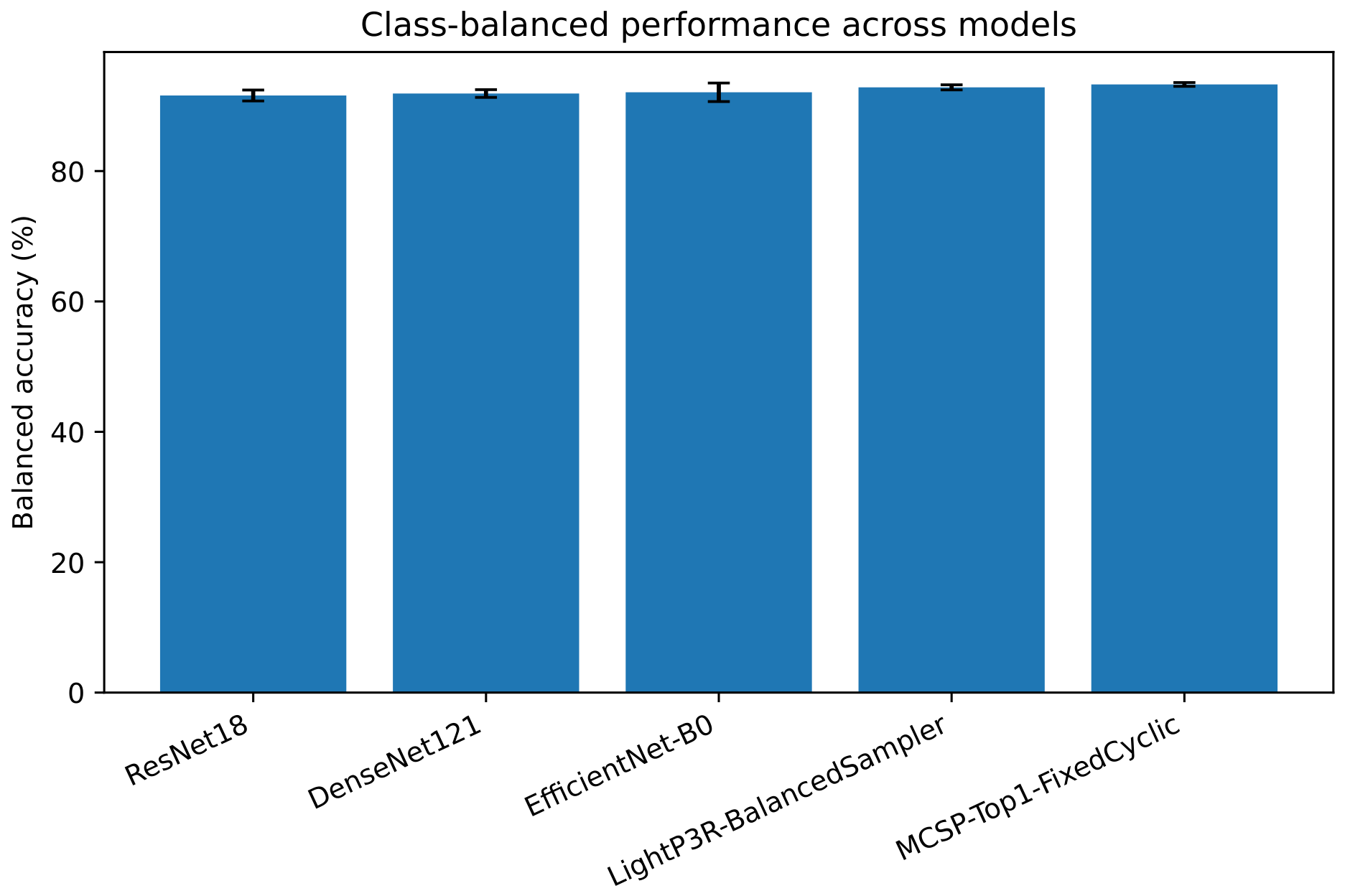
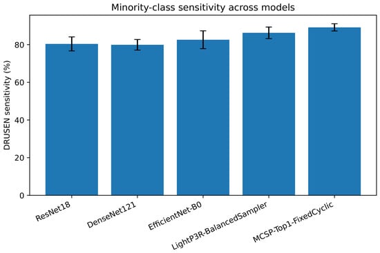
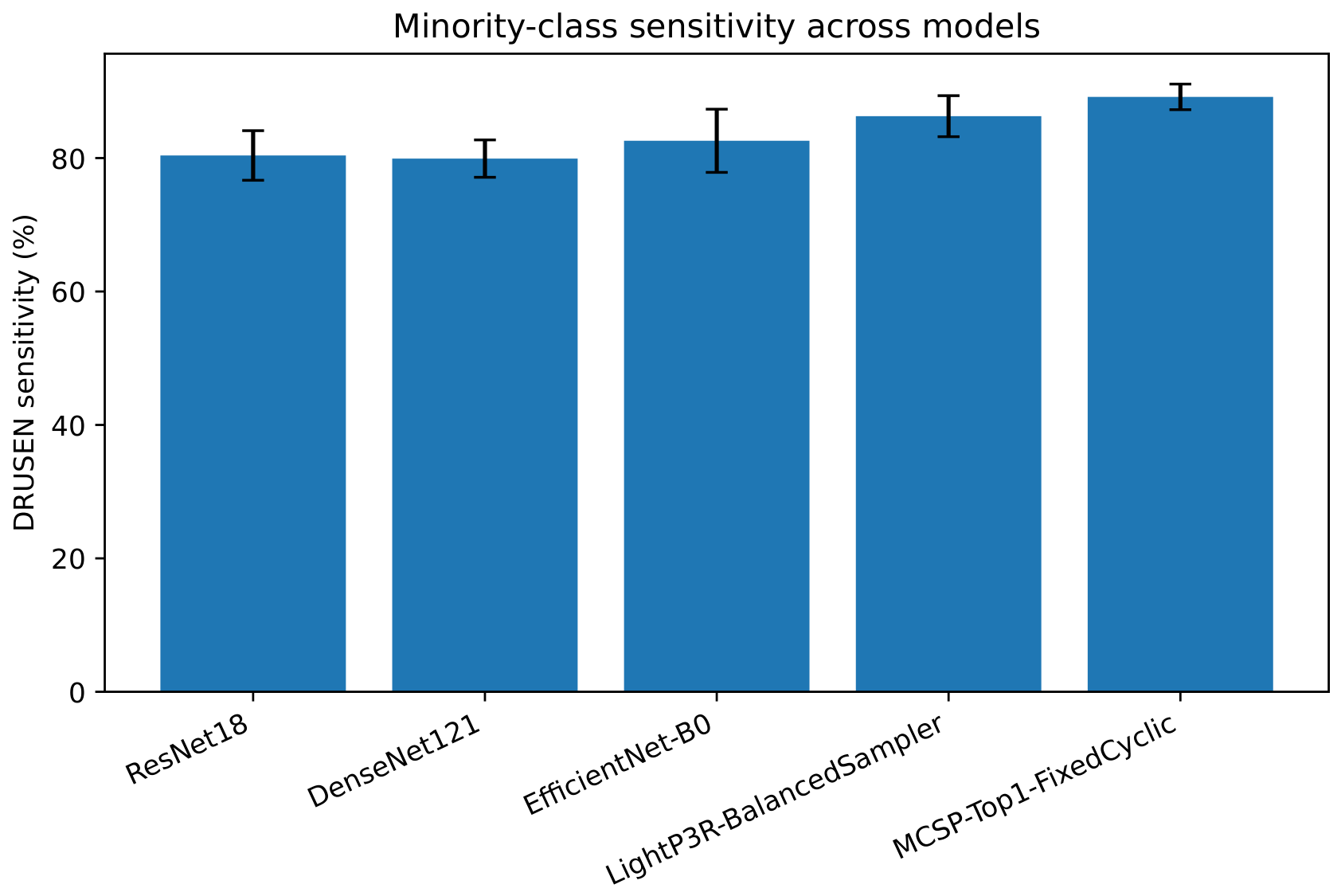
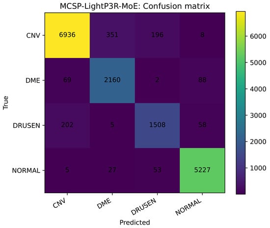
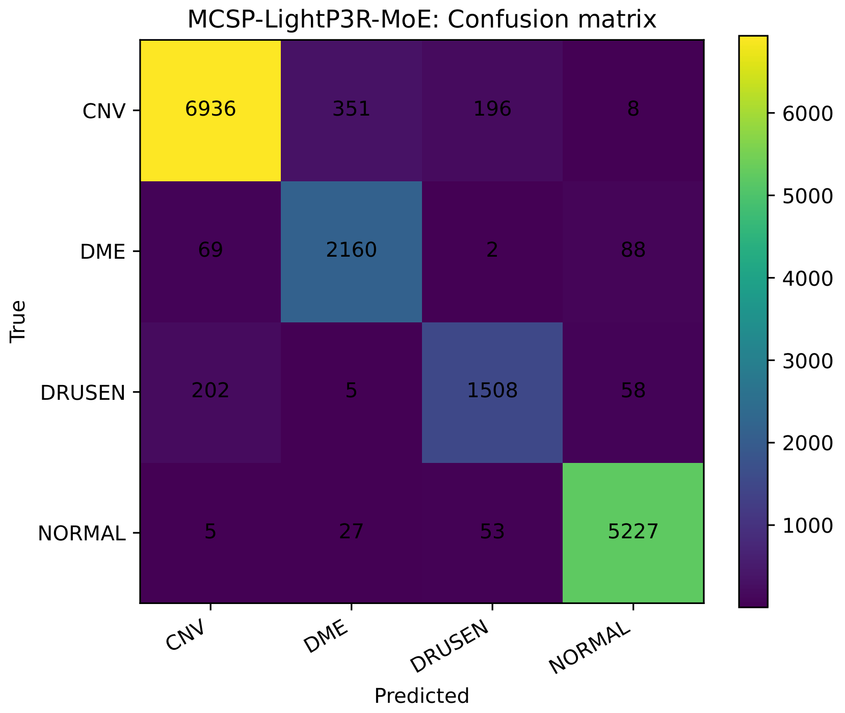
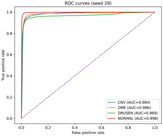
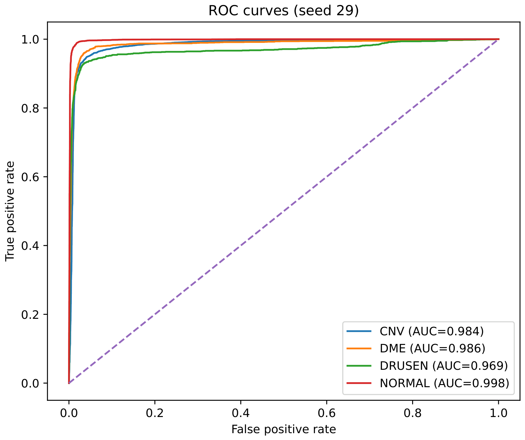
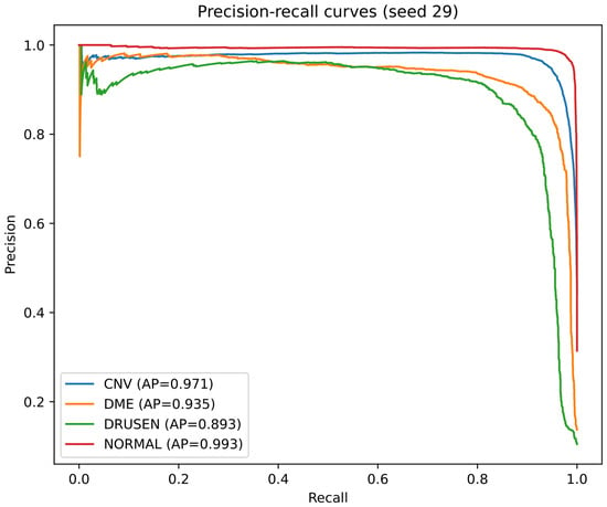
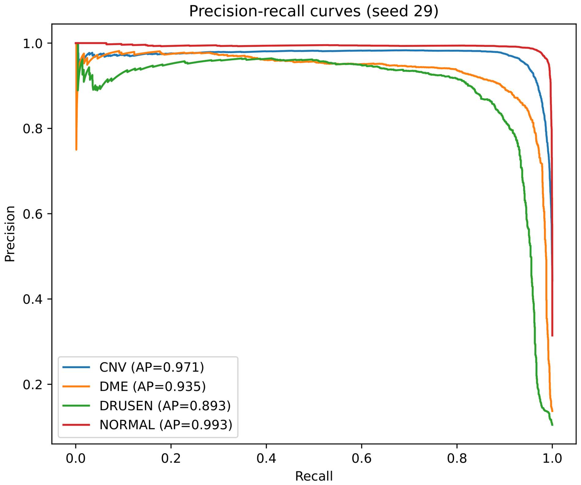
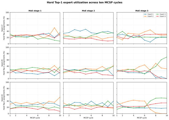
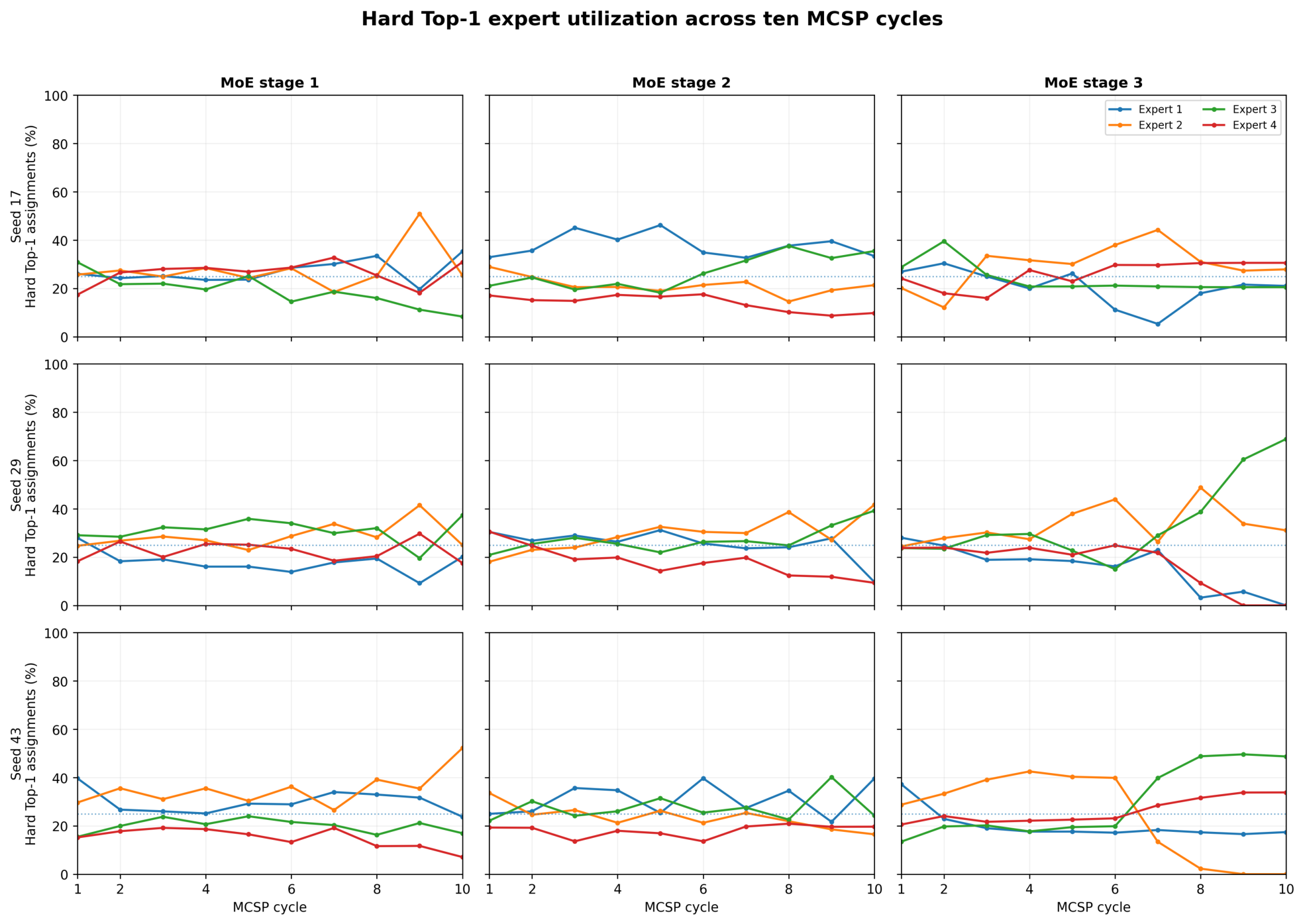
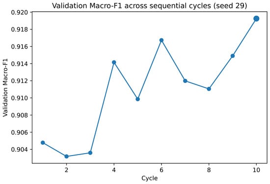
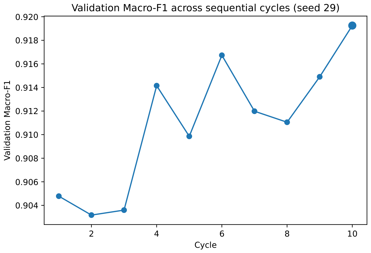

Disclaimer/Publisher’s Note: The statements, opinions and data contained in all publications are solely those of the individual author(s) and contributor(s) and not of MDPI and/or the editor(s). MDPI and/or the editor(s) disclaim responsibility for any injury to people or property resulting from any ideas, methods, instructions or products referred to in the content. |
© 2026 by the authors. Licensee MDPI, Basel, Switzerland. This article is an open access article distributed under the terms and conditions of the Creative Commons Attribution (CC BY) license.