Stream Reduction in Multi-Stream Graph Convolutional Networks: A Non-Inferiority Study for Skeleton-Based Action Recognition

Abstract

Multi-stream graph convolutional networks improve skeleton action recognition by combining representations, but each branch adds inference cost. We evaluate one fixed stream-removal operating point in a CTR-GCN pipeline using a paired non-inferiority protocol on NTU RGB+D 120. A temporal configuration reduced source-frame entries requested from the skeleton store by 53.52%, but lost 3.191 percentage points of accuracy and provided no latency saving after reopening the data mapping. A three-stream configuration then omitted bone motion while retaining 64 temporal positions. Historical RTX 4090 measurements at batch size one, using development checkpoints, showed 24.30–24.94% lower latency. After development confirmation, the fixed pair was trained on 54,468 examples and evaluated on 59,477 cross-setup test examples. Overall accuracy was 89.1050% for four streams and 89.0277% for three streams; paired setup-bootstrap lower bounds exceeded all three prespecified non-inferiority margins. Stream removal introduced 605 errors and corrected 559, while predicted labels changed for 1778 examples. Thus, a net loss of 46 correct decisions concealed broader redistribution. Recall decreased for 61 of 120 actions. These findings support assessing a branch by its contribution to the complete system, measured cost, and explicit quality tolerances. They do not imply preservation of every action. A separate CPU experiment with the final checkpoints measured 24.67% mean latency saving across three processes on one host. The contribution is a controlled empirical assessment, not a new architecture.

1. Introduction

Skeleton-based action recognition represents a person’s movement as a sequence of articulated joint positions. This compact description separates much of the motion information from appearance and is useful when the task concerns how a person moves rather than what the scene looks like. Its computational cost nevertheless depends on more than the size of the input. A multi-stream system may process several transformations of the same skeleton sequence through separate networks. Each branch offers a different view of the action, but also adds a forward pass to the recognition pipeline.

For deployment, the relevant question is whether the contribution of an additional branch justifies its measured cost. A small increase in benchmark accuracy can be useful, yet a system with a tight response-time budget may prefer a simpler operating point if the quality loss is bounded. Conversely, reducing the number of input observations can be ineffective when neural inference, rather than input access, dominates execution. Both possibilities call for an evaluation that pairs recognition quality with a clearly defined timing boundary.

We study the marginal value of skeleton representations in a four-stream CTR-GCN system on NTU RGB+D 120 under the cross-setup protocol. Two interventions act on different parts of the computation: reading fewer source frames and omitting the bone-motion stream while retaining 64 temporal positions. For the stream comparison, the retained models and their relative fusion weights are shared between systems. This isolates the contribution of the omitted branch within the selected ensemble.

The study asks three questions. Does reducing source-frame access produce useful pipeline acceleration? Can a complete stream be removed while meeting explicit tolerances for aggregate quality? How does this simplification redistribute decisions across actions and acquisition setups? We distinguish exploratory selection, a development follow-up under a new training seed schedule, hardware timing, and a final fixed test comparison.

The contribution is a controlled assessment of where computation can be removed from a multi-stream graph-convolution system. We combine measured latency with prespecified tolerances for overall accuracy, accuracy on the additional NTU120 actions, and macro-F1. The comparison distinguishes an ineffective temporal configuration from a useful reduction in stream count. Paired decision analysis then shows why a small aggregate loss does not imply that the systems make the same errors. The resulting protocol and saved-output analysis provide a reproducible way to assess this operating point; a new graph-convolution architecture or statistical estimator is not proposed.

2. Related Work

2.1. Graph Models and Complementary Skeleton Representations

Spatial temporal graph convolutional networks model body joints and their temporal connections directly, avoiding a hand-designed sequence descriptor [1]. Adaptive graph approaches extend this representation by learning graph structure; the two-stream adaptive GCN also uses joint and bone information as complementary inputs [2]. MS-G3D develops multi-scale spatial aggregation and spatial–temporal graph modeling [3]. CTR-GCN refines topology on a channel-wise basis [4]. More recently, BlockGCN has revisited topology and channel grouping within graph convolution [5]. These advances provide the architectural background for the reference used here.

Our four inputs are transformations of the same measured skeleton sequence, not four independently acquired sensor modalities. Joint positions, bone vectors, and their temporal differences emphasize different properties of the motion. Four-stream joint, bone, joint-motion and bone-motion fusion is already established in MS-AAGCN [6]. Their complementarity motivates multi-stream fusion, but does not imply that every stream is equally useful for every action. A paired comparison with shared retained checkpoints isolates the effect of excluding a stream from a particular trained ensemble.

2.2. Efficiency and the Scope of the Present Comparison

Efficient skeleton recognition has been pursued through architectural changes as well as adaptive computation. Shift-GCN uses shift operations to reduce the cost of graph-convolution processing [7]. EfficientGCN combines multiple inputs within an efficient network and uses separable operations and compound scaling [8]. AdaSGN adapts the graph choice to reduce computation [9], whereas HPI-GCN studies re-parameterization and over-parameterization for inference [10]. These methods address different parts of the recognition problem and should not be ranked using latencies obtained on different devices or with different measurement boundaries.

Resource constraints also motivate compact temporal models in industrial monitoring. TinyLSN addresses acoustic pipeline-leak detection at IoT edge nodes [11]; LDS-former uses a lightweight dual-stream transformer for monitoring crack evolution [12]; and distributional knowledge harmonization transfers recognition capability to a compact student [13]. Leak-aware diffusion instead addresses limited labelled signals through data augmentation [14]. These studies provide broader context for resource and data constraints, but are not stream-removal baselines for skeleton recognition.

Architecture-level comparisons do not directly determine the contribution of one branch within a particular trained ensemble. The present work holds the reference architecture and shared models fixed within each stream-comparison pair. Its scope is consequently narrower than a benchmark of efficient architectures: it measures the marginal cost and quality contribution of one branch, after examining a temporal alternative. The added evidence is the separation of development from final testing, the use of predetermined loss tolerances, and a paired analysis that preserves setup-level clustering. Passing the decision rule means that the observed system meets those tolerances under the stated resampling assumptions; it does not prove that the two systems are identical or that the simplification is optimal.

3. Materials and Methods

3.1. Reference Model and System Comparison

Each sample is represented by three-dimensional coordinates for 25 joints and at most two people. Let $x_{t,v}$ denote the coordinates of joint v at output time t, and let $p\left(v\right)$ be its parent in the fixed NTU skeleton graph. Bone vectors are $b_{t,v}=x_{t,v}-x_{t,p\left(v\right)}$. Joint motion and bone motion are first temporal differences, $x_{t+1,v}-x_{t,v}$ and $b_{t+1,v}-b_{t,v}$; their final temporal positions are set to zero. All four inputs, therefore, derive from the same skeleton observations.

The reference has ten graph–temporal blocks, with 64 channels in blocks one to four, 128 in blocks five to seven, and 256 in blocks eight to ten. Temporal stride two is used in blocks five and eight. Adaptive topology is enabled. Global averaging over the remaining temporal, joint, and person dimensions precedes a 120-class linear layer. Dropout is disabled. We use this architecturally matched implementation of CTR-GCN [4] consistently throughout the selected comparison; the training recipe and data processing define a reference experiment rather than a reproduction claim for the original paper’s reported score.

The Full-4 reference contains joint, bone, joint-motion, and bone-motion streams. For sample i, let $z_{is}\in {\mathbb{R}}^{120}$ denote the logits from stream s. The two systems are

$$\begin{array}{cc}\hfill z_i^{\left(4\right)}& =0.3z_{i0}+0.3z_{i1}+0.2z_{i2}+0.2z_{i3},\hfill \end{array}$$

(1)

$$\begin{array}{cc}\hfill z_i^{\left(3\right)}& =0.375z_{i0}+0.375z_{i1}+0.25z_{i2}.\hfill \end{array}$$

(2)

Stream-3 excludes bone motion. The retained three checkpoints are identical between the two systems within each comparison. No fusion weights or temperatures are fitted. The frozen implementation combines logits in float32 with the same operation order for all samples and applies an argmax over all 120 classes.

The retained weights are divided by their original sum, $0.8$. Setting bone motion to zero without normalization gives $u_i=0.3z_{i0}+0.3z_{i1}+0.2z_{i2}$, so $z_i^{\left(3\right)}=1.25u_i$. This positive common factor preserves the argmax in exact arithmetic. Normalization, therefore, has no separate effect on class-decision metrics, apart from possible floating-point rounding. It does change softmax probabilities; no calibration equivalence is claimed. A saved-logit check using float32 weights $(0.3,0.3,0.2,0)$ produced zero argmax disagreements with Stream-3 among all 59,477 test samples and identical values of the three endpoints (Supplementary Section S6).

The temporal development study used base seed 271,828 and separately trained the four streams for $K\in \{8,16,32,64\}$. K64 used crop-and-resize, whereas K8, K16, and K32 used exact uniform sampling. K32 was the prespecified primary temporal configuration; its unsuccessful result was retained. Stream-3 was selected subsequently by exploratory analysis of saved development predictions. Its quality protocol was then frozen before new training with base seed 161,803. Finally, the selected Full-4/Stream-3 pair was fixed before the official XSet evaluation. This chronology separates the exploratory selection from the later checks; it does not recast the entire study as prospectively selected.

3.2. Dataset Partitions and Prior Exposure

The study uses the existing processed skeleton data from NTU RGB+D 120 under the XSet protocol [15,16]. The retained development training partition contains 38,670 samples from 12 setups. Its three held-out folds are $(4,12,18,26)$, $(6,14,22,28)$, and $(8,16,24,32)$. Each sample receives exactly one out-of-fold prediction from a model that was not trained on its setup. The former validation partition contains 15,798 samples from setups $(2,10,20,30)$. It and the XSet test were excluded from the temporal and new-seed out-of-fold experiments.

For final training, the official training population contains 54,468 retained samples: the 38,670 base-training samples followed by the 15,798 former validation samples. The latter are used only for training in this final stage. No metric is computed on them for checkpoint or parameter selection. The final XSet test contains 59,477 retained samples from the 16 odd-numbered setups. Canonical manifests establish the sample order, labels, and setup membership. Their sample IDs are unique and disjoint across the original train, validation, and test partitions. Existing preprocessing is reused.

The retained manifests contain 113,945 unique sequences and exclude all 535 identifiers in the provider’s missing-or-incomplete-skeleton list; these counts reconcile with the nominal 114,480 recordings. Recovered preparation records report 535 ignored recordings and zero logged parsing errors; their three canonical manifest hashes match the archived partitions. The parser tracks body identifiers, retains up to two tracks, stores the first 25 joints’ three-dimensional coordinates as float32, and zero-fills absent observations. Trailing empty frames are excluded from the effective sequence length, while internal empty frames remain. No coordinate centering, scale normalization, or confidence-based joint denoising is added. Supplementary Section S8 specifies track selection, exclusion checks, and the raw-data preparation route, including its provenance limits.

NTU RGB+D 120 extends NTU RGB+D with additional actions [17]. Earlier stages of the project used NTU60, so A1–A60 cannot be presented as independent of the complete research history. A61–A120 provides the strongest held-out interpretation for the final test examples within the documented history. These actions are represented in training; the endpoint is not a zero-shot evaluation. It contains 29,375 test samples in setups 19, 21, 23, 25, 27, 29, and 31. The remaining 30,102 samples belong to A1–A60. All of these evaluations remain within NTU RGB+D 120.

3.3. Training and Temporal Representation

The new-seed development follow-up comprises four streams in each of three folds. Its job seed is 161,803 + $1000(f-1)+10s$, where f is the one-based fold index and s is the zero-based stream index. Final training instead uses four full-training models with seeds 161,803, 161,813, 161,823, and 161,833. The full-training checkpoints are newly fitted models, not an ensemble of the earlier fold checkpoints.

All these trainings use 65 epochs of SGD with batch size 64, initial learning rate 0.1, momentum 0.9, Nesterov acceleration, and weight decay $4\times {10}^{-4}$. The learning rate has five warm-up epochs and reductions by a factor of 0.1 at epochs 35 and 55. Label smoothing and automatic mixed precision are disabled. The final epoch is retained without validation monitoring. Deterministic algorithms are requested in warning mode; bitwise agreement across arbitrary hardware and software environments is not claimed.

K64 uses 64 output frames with crop-and-resize temporal interpolation. Training uses a random crop proportion in $[0.5,1.0]$ and rotation augmentation with independent angles sampled uniformly from $[-0.3,0.3]$ radians around each axis. Evaluation uses a centered crop with proportion 0.95 and no rotation. The sparse adapter reads the interpolation supports from the existing skeleton store. In final training, base-training samples use that store, while former-validation samples use the existing processed NPZ files with the same support and interpolation operations. Final test samples use the NPZ adapter. The preflight records exact tensor and temporal-index parity on 432 prescribed base-training cases; no test tensor is used for that parity check.

3.4. Final Evaluation and Numerical Reproduction

All four final models were trained before evaluating the selected system pair. Their identities, the data partitions, the fusion rules, and the analysis protocol were fixed before the final test evaluation. One saved prediction matrix per stream supplies both systems. Stream-3 reuses the retained three streams; no second forward pass or separate checkpoint selection is involved.

The analysis checks sample identifiers, class labels, setup labels, and temporal-position metadata across the four prediction files. It then reconstructs both fused outputs and all reported endpoints. A separate implementation uses per-setup class counts to reproduce the bootstrap, providing a check against the original confusion-matrix implementation. This verifies the saved-output calculations without rerunning training or inference. Supplementary Materials describe the evidence coverage and the distinction between reproducing an analysis and reproducing model training. Supplementary Section S9 maps the main-text tables and figures to archived inputs and executable CPU commands. Historical temporal and development tables are regenerated from retained summary records; final endpoints and historical stream latency can additionally be recomputed from predictions and timing traces. The revision supplement supplies the new sensitivity scripts and their input hashes.

3.5. Quality Criteria and Paired Bootstrap

The three quality endpoints are overall Top-1, Top-1 on A61–A120, and macro-F1 over all 120 classes. Let ${\widehat{\Delta }}_j$ be Stream-3 minus Full-4 for endpoint j. The fixed non-inferiority margins on the unit scale are $m=(-0.010,-0.015,-0.015)$. These tolerances define the study’s decision rule; they are not universal tolerances for every application or action. Non-inferiority is assessed against an explicitly chosen margin rather than inferred from a nonsignificant difference [18]. The margins here are operational study choices; they were not derived from a user study or a domain-specific cost model.

The bootstrap [19] approximates sampling variation by resampling acquisition setups as clusters, while preserving the pairing of the two systems. Resampling clusters rather than individual sequences reflects the grouping imposed by the XSet evaluation, although it cannot remove all dependence between subjects recorded in different setups. A paired setup-cluster bootstrap resamples setups with replacement and includes all samples from each selected setup with the selected multiplicity. Both systems use the same replicate. Preserving dependence and pairing is central to interpretable resampling for comparative measurements [20]. Accuracy is computed over the resulting sample union, not as an equally weighted average of setup accuracies. Macro-F1 is recalculated within each replicate as

$$F_{\mathrm{macro}}={\displaystyle \frac{1}{120}}{\displaystyle \sum _{c=1}^{120}}{\displaystyle \frac{2T{P}_c}{N_c+{\widehat{N}}_c}},$$

(3)

where $N_c$ and ${\widehat{N}}_c$ are true and predicted class counts. A term with zero denominator is set to zero. The class set is not reduced when a bootstrap draw lacks support for an action.

The development follow-up resamples its 12 setups. The final protocol uses 10,000 replicates of the 16 test setups. A pool of 20,000 index rows is frozen with seed 223,607. Before training, canonical test metadata select the first 10,000 rows with nonzero A61–A120 support; no prediction is used in this selection. The actual selected pool required no rejected rows. The saved index array and its raw little-endian int64 hash are verified independently during the audit.

With ${\alpha }_j=0.05/3$, the one-sided centered-basic lower bound is

$$L_j=2{\widehat{\Delta }}_j-Q_{1-{\alpha }_j}\left({\widehat{\Delta }}_j^{*}\right),$$

(4)

using the higher empirical quantile. Non-inferiority is established under the study rule only if $L_j>m_j$ for all three endpoints. The frozen Bonferroni allocation is retained throughout. The corresponding resampling p-value is

$$p_j={\displaystyle \frac{1+{\sum }_{b=1}^B\mathbf{1}\{{\widehat{\Delta }}_{jb}^{*}-{\widehat{\Delta }}_j\ge {\widehat{\Delta }}_j-m_j\}}{B+1}},B=\mathrm{10,000},$$

(5)

with adjusted value $min(1,3p_j)$. These are approximate cluster-bootstrap inferences conditional on the fitted models. Setup and class summaries are descriptive and cannot alter the criteria, margins, candidate, or checkpoint. Setup clustering reflects the acquisition-based XSet split and avoids treating all clips as independent replicates. However, 16 setups, especially the seven supporting A61–A120, provide limited information for resampling. More bootstrap draws improve simulation resolution but do not establish nominal coverage with so few clusters.

3.6. Latency Measurement

The Stream-3 latency experiment used the existing seed-271,828 checkpoints, an RTX 4090 (NVIDIA Corporation, Santa Clara, CA, USA), and batch size one. Eighteen paired traces cover three folds, two mapping regimes, and three process repetitions. Each trace has 400 samples, with 100 from each held-out setup, after 30 warm-up samples per system. For each sample and system, the median of the three process repetitions is computed first; reported latency is then the mean of those per-sample medians over 1200 samples in each regime. Its separate setup-cluster procedure resamples these aggregated paired observations and adjusts for the two latency endpoints. The resulting bounds do not include the full variability between processes or devices. The prespecified requirement is a one-sided lower bound greater than 20% saving in both regimes.

Timing begins at dataset sample access and includes skeleton preparation, modality construction, host-to-device transfer, sequential network forwards, weighted fusion, argmax, and CUDA synchronization. Model loading and dataset-object construction are excluded. Warm reuse means that the same dataset object and its existing file mapping are retained between accesses. Fresh mapping means that a new dataset object and file mapping are constructed before timing starts; these construction costs are excluded. Reopening the mapping does not flush the operating-system page cache, so this regime is not a cold-disk benchmark. The latency and quality stages use different seed-specific checkpoints with the same architecture and stream composition. The reported timing is consequently historical evidence for this architecture and stream composition; it is not a direct accuracy–latency measurement of the final fitted pair. Temporal and stream-reduction campaigns retain their own paired Full-4 references; their absolute timings are not pooled.

A separate revision-stage experiment measured the four final checkpoints on an AMD Ryzen 7 7840HS CPU (Advanced Micro Devices, Inc., Santa Clara, CA, USA). The protocol and cohort were fixed before measurement: 64 former-validation examples from the official training population, 16 from each of setups 2, 10, 20, and 30, selected deterministically by sample-ID hashes. At batch size one and float32, with one intra-operation and one inter-operation thread, each of three fresh processes ran 10 warm-up pairs and 64 measured pairs, alternating system order. Timing covered resident raw skeleton arrays, canonical K64 resampling, required modalities, sequential forwards, fixed fusion, and argmax. Disk access, NPZ decoding, integrity checks, model loading, and pose estimation were excluded. Stream-3 recomputed its three forwards rather than reusing Full-4 outputs. We report the mean and sample standard deviation of process-level means, not confidence intervals. Supplementary Section S10 gives the environment, results, and input provenance. This experiment performed no training, accuracy calculation, or test-set forward pass. Historical GPU timing used Python 3.11.16, PyTorch 2.11.0+cu128 (CUDA 12.8), and NumPy 2.4.6; the final-checkpoint CPU measurement used Python 3.11.8, PyTorch 2.11.0+cpu, and NumPy 2.3.5. Further environment details are provided in Supplementary Sections S9 and S10.

3.7. Use of Generative AI Tools

ChatGPT (OpenAI; model label: GPT Astra Ultra) and Codex (OpenAI; integrated assistance in ChatGPT Work Mode; exact version not recorded) assisted with code development and debugging, implementation and checking of analysis scripts, interpretation of results, and drafting and revision of the manuscript. The reported performance values were obtained from the experimental pipelines and saved prediction and timing files. Numerical verification included recomputing the fixed fusion, evaluation metrics, and bootstrap outputs from the archived artifacts. The code and research artifacts are publicly available at https://doi.org/10.5281/zenodo.22858090.

4. Results

4.1. Temporal Reduction Did Not Meet the Efficiency Criterion

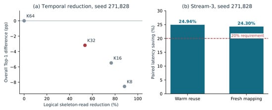
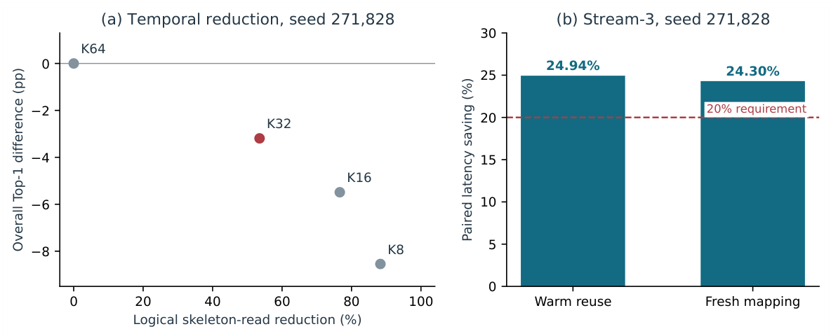
A logical skeleton read is a source-frame entry requested by the temporal adapter, rather than a physical disk transaction. The primary K32 configuration reduced the mean number of these reads by 53.52%, but decreased overall Top-1 by 3.191 percentage points and produced $-0.100\%$ fresh-mapping latency saving (Table 1). K16 and K8 further reduced reads while losing more accuracy; their measured savings remained below one percent. The lower-K points remain historical secondary configurations and do not redefine the primary K32 result. Logical source access is a property of the skeleton store, not a measurement of RGB acquisition or sensor energy. This comparison changes the temporal representation as well as its length: K64 uses crop-and-resize interpolation, whereas K32 uses exact uniform sampling. Motion features are differences between consecutive sampled positions without division by elapsed time. The observed loss, therefore, applies to this combined sampling and motion-feature recipe; it does not establish that reducing frame count alone is ineffective.

Table 1. Temporal development results, seed 271,828. Each variant was trained separately. Latency saving uses the paired reference from that campaign. K64 and the lower-K variants also use different temporal resampling rules.

Variant	All Top-1 (%)	A61–A120 (%)	Read Reduction (%)	Saving (%)
K64 resize	83.659	81.191	0.00	0.000
K32 exact	80.468	76.773	53.52	−0.100
K16 exact	78.172	74.744	76.62	0.036
K8 exact	75.115	72.966	88.31	0.477

The saved fresh-mapping profile records 56.177438 ms for the reference and 55.2887745 ms for K32 inference alone. If this inference time stays fixed and all remaining overhead is idealized as zero, the saving ceiling is

$$1-{\displaystyle \frac{55.2887745}{56.177438}}=1.5819\%.$$

(6)

The analogous warm-reuse value is 0.8849%. These are conditional diagnostics from aggregated timings, not confidence bounds or hardware-independent limits. The temporal-representation confounding described above also limits interpretation of this profile. Separately aggregated stage timings need not sum exactly to an aggregated total.

4.2. Measured Latency of the Three-Stream System

For the historical seed-271,828 development checkpoints, warm-reuse latency fell from 65.2755 to 48.9959 ms and fresh-mapping latency from 68.5097 to 51.8634 ms (Table 2). The savings were 24.9399% and 24.2977%, respectively. Both lower bounds exceeded 20%. Figure 1 presents the temporal quality cost and the separately measured stream-reduction latency benefit. Across the three processes within each fold and mapping regime, the sample standard deviation of percentage saving was 0.079–0.241 percentage points. Supplementary Table S7 reports the process-level means and standard deviations separately from the original median-per-sample estimator; it describes the historical GPU campaign separately from the final-checkpoint CPU measurement below.

Table 2. Earlier Stream-3 latency measurements: RTX 4090, batch one, seed-271,828 checkpoints. Final checkpoints were measured separately on CPU, not remeasured on this GPU.

Regime	Full-4 (ms)	Stream-3 (ms)	Saving (%)	Lower Bound (%)
Warm reuse	65.2755	48.9959	24.9399	24.8819
Fresh mapping	68.5097	51.8634	24.2977	24.2223

Figure 1. Historical interventions. (a) Greater logical-read reduction was associated with larger accuracy loss in the temporal configurations. (b) Stream-3 met both latency requirements in its separate measurement campaign. Panel (a) does not imply that read reduction is a latency measurement. The red marker identifies K32, the prespecified primary temporal configuration.

For the final checkpoints on the Ryzen 7 7840HS, Full-4 and Stream-3 mean latencies were $764.3\pm 5.0$ and $575.7\pm 4.5$ ms, respectively, where the spread is the sample standard deviation across three process means. Mean percentage saving was 24.67%, with a standard deviation of 0.62 percentage points and a process range of 23.96–25.06% (Supplementary Table S9). These results concern a resident-input, single-thread CPU pipeline on one host. The similar relative saving to the historical GPU result is descriptive; different checkpoints, inputs, environments, and timing boundaries preclude a direct cross-device latency comparison.

4.3. Development Confirmation Under a New Seed Schedule

The frozen follow-up met all three non-inferiority criteria (Table 3). Full-4 correctly classified 32,393 of 38,670 samples and Stream-3 classified 32,259. There were 600 correct-to-error transitions and 466 error-to-correct transitions, giving 134 additional errors. Fold differences in overall Top-1 were $-0.024$, $-0.279$, and $-0.707$ percentage points. These results support repeatability under the new training seed schedule on the same development samples and fold plan. They are not an independent-dataset test.

Table 3. Development confirmation, base seed 161,803. Metrics are percentages; differences, lower bounds, and margins are percentage points.

Endpoint	Full-4	Stream-3	Difference	Lower Bound	Margin
Overall Top-1	83.768	83.421	−0.347	−0.661	−1.000
A61–A120 Top-1	81.722	81.632	−0.089	−0.546	−1.500
Macro-F1	83.791	83.456	−0.335	−0.601	−1.500

4.4. Final Cross-Setup Evaluation

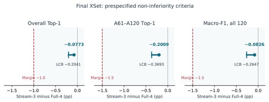
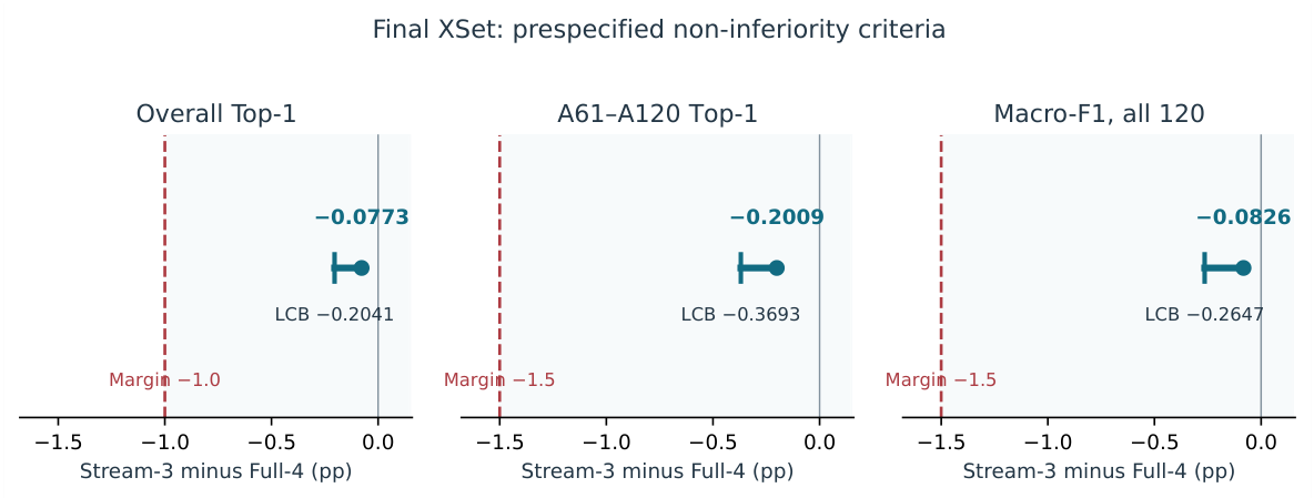
The final paired comparison met all three prespecified non-inferiority criteria (Table 4; Figure 2). Overall Top-1 was 89.1050% for Full-4 and 89.0277% for Stream-3. The difference was $-0.0773$ percentage points, with a lower bound of $-0.2041$ percentage points against the $-1.0$ margin. For A61–A120, the difference was $-0.2009$ percentage points and its lower bound was $-0.3693$, against the $-1.5$ margin. Macro-F1 decreased by 0.0826 percentage points, with a lower bound of $-0.2647$, also above $-1.5$.

Table 4. Final paired XSet comparison from the four saved stream logit files. Metrics are percentages; differences, lower bounds, and margins are percentage points. All three criteria are met.

Endpoint	Full-4	Stream-3	Difference	Lower Bound	Margin
Overall Top-1	89.1050	89.0277	−0.0773	−0.2041	−1.0000
A61–A120 Top-1	87.0672	86.8664	−0.2009	−0.3693	−1.5000
Macro-F1, all 120	89.1059	89.0233	−0.0826	−0.2647	−1.5000

Figure 2. Final quality criteria. Each segment connects a one-sided lower bound to the point estimate; it is not a two-sided confidence interval. Dashed lines show the unchanged margins.

All three adjusted resampling p-values were 0.0002999700. The underlying value 1/10,001 is the minimum permitted by the implemented finite-resample formula; it is not a claim of zero probability. The decision follows the frozen lower-bound rule.

Post hoc sensitivity checks preserve the frozen analysis (Supplementary Section S6). All three existing lower bounds also exceed a common loss margin of $-0.5$ percentage points; at $-0.25$, only overall Top-1 meets the criterion. Leaving out each setup in turn gives difference ranges of $-0.1007$ to $-0.0388$ percentage points for overall Top-1, $-0.2420$ to $-0.1417$ for A61–A120, and $-0.1104$ to $-0.0315$ for macro-F1. These point-estimate diagnostics show limited influence of any single observed setup; they are not confidence intervals or evidence of nominal bootstrap coverage with seven contributing setups.

Full-4 produced 52,997 correct decisions and Stream-3 produced 52,951. Stream removal changed 605 correct decisions into errors and corrected 559 reference errors. The net cost was 46 additional errors, or 0.7734 per 1000 test samples. For A61–A120, the counts were 25,576 and 25,517 among 29,375 samples: 59 fewer correct decisions. For A1–A60, the counts were 27,421 and 27,434 among 30,102 samples: 13 more correct decisions. These group counts describe the distribution of the aggregate effect and do not define another selection or testing stage.

The small accuracy difference results from opposing changes rather than identical decisions (Table 5). Predicted labels changed for 1778 examples (2.9894%). Correctness changed for 1164 of them: 605 newly incorrect and 559 newly correct. In the other 614 cases, both systems were incorrect but selected different labels. Among the 5921 examples misclassified by both systems, 5307 retained the same wrong label. These counts describe decision redistribution without introducing a further hypothesis test. Complete class-pair transitions are included in the accompanying numerical results.

Table 5. Paired correctness of the two fixed systems on all 59,477 test examples. Rows refer to Full-4 and columns to Stream-3. The off-diagonal entries distinguish introduced from corrected errors.

Full-4 Outcome	Stream-3 Correct	Stream-3 Incorrect	Total
Correct	52,392	605	52,997
Incorrect	559	5921	6480
Total	52,951	6526	59,477

4.5. Variation Across Setups and Action Classes

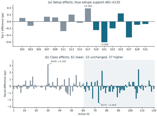
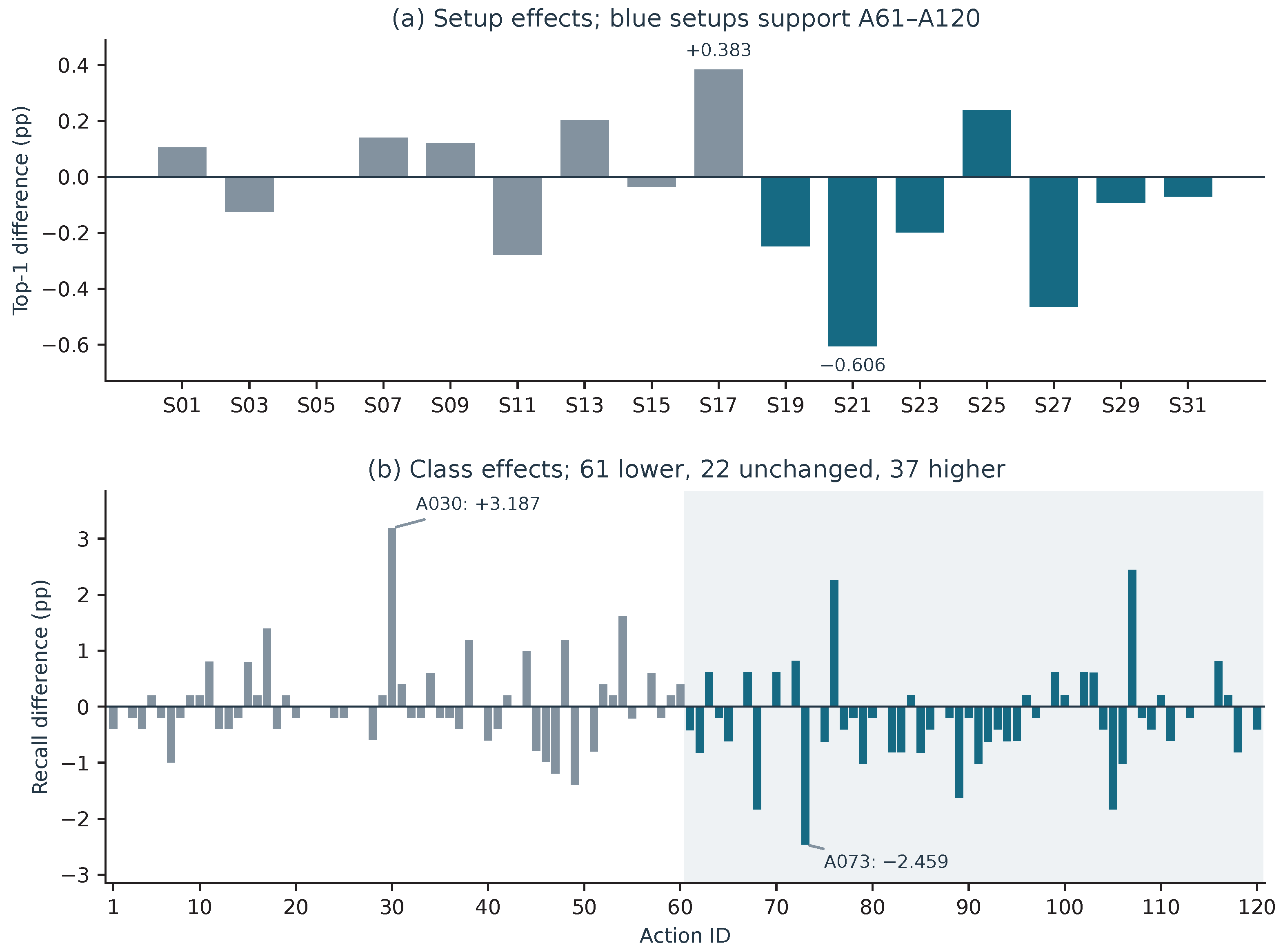
Setup-level overall Top-1 differences ranged from $-0.6063$ percentage points in S21 to $+0.3834$ in S17. Class recall decreased for 61 actions, was unchanged for 22, and increased for 37. The largest decrease was A073, with 12 fewer correct decisions among 488 samples ($-2.4590$ percentage points). The largest increase was A030, with 16 more correct decisions among 502 samples ($+3.1873$ percentage points). These extrema were identified descriptively after the results. They are not multiplicity- adjusted class claims. Figure 3 and Supplementary Tables S1 and S2 report the effects without changing the aggregate decision rule.

Figure 3. Descriptive final-test heterogeneity. Blue denotes the setups or actions supporting A61–A120; gray denotes the earlier action group. The two panels concern different metrics: Top-1 by setup and recall by class. No additional inferential claim is drawn from these slices.

The five largest recall decreases concern A073 (staple book, $-2.459$ percentage points), A068 (flick hair, $-1.837$), A105 (blow nose, $-1.833$), A089 (put object into bag, $-1.629$), and A049 (fan self, $-1.392$); action names follow the dataset documentation [17]. These actions involve upper-limb motion, often with object or hand–face interaction, for which changing limb configuration could be informative. Yet A076 (cutting paper), another hand–object action, improves by $2.254$ percentage points. This descriptive pattern suggests a question for localized motion analysis, rather than establishing a common failure mechanism or a semantic group that uniquely requires bone motion.

5. Discussion

The two interventions act on different parts of the computation. Temporal reduction changes source access and the number of input positions, whereas removing a stream eliminates a complete network evaluation. In the recorded profile, inference latency changed little despite temporal reduction, and inference still accounted for most of the measured time. These observations account for the small end-to-end saving in this implementation; the profile does not isolate a hardware-level cause. Removing one sequential stream reduced latency by approximately one quarter in the historical GPU campaign and in the separate final-checkpoint CPU experiment. The same ordering need not hold when video decoding, pose estimation, or data transfer contributes substantially to total cost. Moreover, the temporal comparison changes both the number of observations and their resampling rule; it does not isolate a universal effect of frame count.

5.1. Implications for Multi-Stream GNN Design

The omitted bone-motion branch is not the weakest standalone classifier in the final evaluation: its Top-1 accuracy is 82.0183%, compared with 81.4483% for joints and 81.9695% for joint motion. Standalone accuracy, therefore, does not determine a branch’s marginal contribution to the ensemble. The paired results assess that contribution through changes in the decisions of the complete system. They support evaluating representations jointly with the retained branches and the fixed fusion rule, rather than ranking them only as separate classifiers.

The net accuracy difference corresponds to fewer than one additional error per 1000 examples, but nearly 30 predicted labels per 1000 examples changed. This distinction matters when errors have unequal consequences. The observed balance of corrected and introduced errors may be acceptable for one application and unacceptable for another, especially when an affected action is important. Aggregate non-inferiority and class-level descriptions answer different questions and should be reported together.

For a new application, the practical sequence is to profile the actual timing boundary, specify acceptable quality losses before evaluating the final candidate, and then inspect the paired error changes alongside aggregate metrics. Shared retained checkpoints make the comparison interpretable by avoiding an additional source of training variation between the two systems. Our experiment demonstrates this assessment for a single selected stream reduction; it does not show that the same branch should be removed from every multi-stream GNN.

MS-G3D and BlockGCN use different spatial–temporal aggregation and topology organization [3,5], potentially changing the complementarity of the streams. Omitting joints or joint motion would also change the retained information. The paired assessment with shared checkpoints and fixed tolerances transfers to these comparisons; the present non-inferiority outcome does not transfer without evaluation.

Skeleton coordinates and their differences are also signals supported on a body graph. Community-based partition-of-unity interpolation [21] offers a complementary perspective on localized graph-signal processing, not an action-recognition baseline. It motivates asking whether bone motion adds information mainly in particular body regions, which could support part-dependent computation. This remains a hypothesis: our class-level results neither locate informative joints nor demonstrate savings from localized computation.

Skeleton recognition is one component of action analysis in video streams. Reducing its cost may help when several cameras or sequences must share a computing budget. The present experiments use presegmented clips and provided skeleton coordinates. They do not measure pose estimation, action localization in continuous video, or operation on an embedded device. Evaluating these stages together is necessary before extending the findings to a complete video-analysis system.

5.2. Limits of the Evidence

The final Top-1 values are higher than the development values, but this change cannot be attributed solely to a better operating point. The final models use a larger training population and a different evaluation population. Only the paired Full-4/Stream-3 comparison within each stage has the stated controlled interpretation. Combining fold checkpoints into an additional ensemble would also change the number of forwards and would define another system; that option was not used.

The held-out evidence remains within NTU RGB+D 120. Earlier NTU60 work limits the interpretation of A1–A60 as untouched by the project history. A61–A120 is, therefore, the stronger held-out component, but it contains samples from only seven setups. Even with 29,375 samples, the effective cluster count for that endpoint remains small. Cluster-bootstrap inference is approximate and conditional on these fitted models. It does not quantify training variability over many independent seeds, subject-level dependence across setups, or uncertainty on another dataset.

Non-inferiority is defined by the fixed margins. It does not imply equality, general equivalence, or preservation of each action. The 61 decreases in class recall and the worst-class decrease of 2.4590 percentage points are material limits of an aggregate claim. An application that places special weight on an affected action could reach a different practical assessment without changing the scientific result of this prespecified comparison. For accuracy, margins of 1.0 and 1.5 percentage points allow losses of 10 and 15 correct decisions per 1000 examples in the respective populations; macro-F1 has no direct error-count equivalent. They do not price specific mistakes. Recall for A043 (falling down) is unchanged, but A045 (chest pain) and A047 (neck pain) lose 0.794 and 1.190 percentage points. Safety-critical use, therefore, requires separately justified requirements for critical actions and validation in the intended setting; aggregate non-inferiority provides no safety guarantee.

Latency was measured in one RTX 4090 environment (NVIDIA Corporation, Santa Clara, CA, USA) using development checkpoints and separately on one Ryzen 7 7840HS CPU using final checkpoints, both at batch size one. The CPU experiment addresses final-model timing on that host but does not repeat the GPU experiment under matched conditions. Its three process repetitions estimate descriptive process variation, not host-to-host variation or a confidence interval. The mean Stream-3 latency of about 0.576 s per presegmented sequence on this single-thread CPU path does not establish real-time performance. Both systems retained all four loaded models in memory, so memory savings were not measured. The study measures neither energy nor batched throughput, and neither environment establishes suitability on an embedded or mobile platform.

The numerical reproduction establishes the consistency of the supplied final evidence. It does not replay training or test inference. A matched comparison with efficient architectures, a broader seed study, and measurements on additional devices would be required to assess whether the observed operating point remains competitive outside this implementation. No superiority over EfficientGCN, HPI-GCN, or other published recognition systems is established.

6. Conclusions

This study provides a controlled non-inferiority assessment of one bone-motion-removal operating point in a fixed CTR-GCN pipeline, rather than a new architecture or a universal stream-selection rule. The tested temporal sampling and motion-feature recipe lowered source-frame access but did not meet the required latency–quality trade-off. Historical development-checkpoint measurements showed 24.30–24.94% lower batch-one latency after bone-motion removal from the K64 system. The final fixed three-stream comparison then met all three prespecified aggregate non-inferiority criteria on NTU120 XSet, with 46 fewer correct predictions among 59,477 examples.

The small net loss combined 605 introduced and 559 corrected errors; a further 614 predictions changed between incorrect labels. These changes explain why aggregate quality tolerances must be interpreted together with class-level effects. The study provides a reproducible evaluation protocol and empirical guidance for this stream-reduction choice. Its extension to other backbones, independently trained systems, devices, and complete video pipelines remains to be tested. A separate final-checkpoint CPU measurement showed 24.67% mean latency saving under its stated resident-input boundary; it does not establish equivalent gains across devices or complete video pipelines.

References

- Yan, S.; Xiong, Y.; Lin, D. Spatial Temporal Graph Convolutional Networks for Skeleton-Based Action Recognition. In Proceedings of the AAAI Conference on Artificial Intelligence; AAAI Press: Palo Alto, CA, USA, 2018; Volume 32. [Google Scholar] [CrossRef] [Scilit]
- Shi, L.; Zhang, Y.; Cheng, J.; Lu, H. Two-Stream Adaptive Graph Convolutional Networks for Skeleton-Based Action Recognition. In Proceedings of the IEEE/CVF Conference on Computer Vision and Pattern Recognition; IEEE: Piscataway, NJ, USA, 2019; pp. 12026–12035. [Google Scholar]
- Liu, Z.; Zhang, H.; Chen, Z.; Wang, Z.; Ouyang, W. Disentangling and Unifying Graph Convolutions for Skeleton-Based Action Recognition. In Proceedings of the IEEE/CVF Conference on Computer Vision and Pattern Recognition; IEEE: Piscataway, NJ, USA, 2020; pp. 143–152. [Google Scholar]
- Chen, Y.; Zhang, Z.; Yuan, C.; Li, B.; Deng, Y.; Hu, W. Channel-wise Topology Refinement Graph Convolution for Skeleton-Based Action Recognition. In Proceedings of the IEEE/CVF International Conference on Computer Vision; IEEE: Piscataway, NJ, USA, 2021; pp. 13359–13368. [Google Scholar]
- Zhou, Y.; Yan, X.; Cheng, Z.Q.; Yan, Y.; Dai, Q.; Hua, X.S. BlockGCN: Redefine Topology Awareness for Skeleton-Based Action Recognition. In Proceedings of the IEEE/CVF Conference on Computer Vision and Pattern Recognition; IEEE: Piscataway, NJ, USA, 2024; pp. 2049–2058. [Google Scholar] [CrossRef] [Scilit]
- Shi, L.; Zhang, Y.; Cheng, J.; Lu, H. Skeleton-Based Action Recognition with Multi-Stream Adaptive Graph Convolutional Networks. IEEE Trans. Image Process. 2020, 29, 9532–9545. [Google Scholar] [CrossRef] [Scilit] [PubMed]
- Cheng, K.; Zhang, Y.; He, X.; Chen, W.; Cheng, J.; Lu, H. Skeleton-Based Action Recognition with Shift Graph Convolutional Network. In Proceedings of the IEEE/CVF Conference on Computer Vision and Pattern Recognition; IEEE: Piscataway, NJ, USA, 2020; pp. 183–192. [Google Scholar]
- Song, Y.F.; Zhang, Z.; Shan, C.; Wang, L. Constructing Stronger and Faster Baselines for Skeleton-Based Action Recognition. IEEE Trans. Pattern Anal. Mach. Intell. 2023, 45, 1474–1488. [Google Scholar] [CrossRef] [Scilit] [PubMed]
- Shi, L.; Zhang, Y.; Cheng, J.; Lu, H. AdaSGN: Adapting Joint Number and Model Size for Efficient Skeleton-Based Action Recognition. In Proceedings of the IEEE/CVF International Conference on Computer Vision; IEEE: Piscataway, NJ, USA, 2021; pp. 13413–13422. [Google Scholar]
- Wang, J.; Li, Z.; Liu, B.; Cai, H.; Saada, M.; Meng, Q. High-Performance Inference Graph Convolutional Networks for Skeleton-Based Action Recognition. Neurocomputing 2025, 653, 131078. [Google Scholar] [CrossRef] [Scilit]
- Lu, Y.; Zhang, Y.; Liu, H.; Bader, S. TinyLSN: A Lightweight Network for Real-Time Marine Pipeline Leakage Detection in IoT Systems. IEEE Internet Things J. 2026, 13, 21104–21116. [Google Scholar] [CrossRef] [Scilit]
- Lu, Y.; Zhu, Z.; Li, Y.; Liu, H.; Hou, J.; Zhou, C.; Abdel Wahab, M. LDS-former: A Lightweight Dual-Stream Transformer for Real-Time Acoustic Emission Monitoring of Crack Evolution in Offshore Steel Structures. Adv. Eng. Inform. 2026, 74, 104635. [Google Scholar] [CrossRef] [Scilit]
- Lu, Y.; Zhang, Y.; Liu, H.; Zhang, X.; Bader, S.; Rahardja, S. A Novel Lightweight Distributional Knowledge Harmonization Framework for Acoustic Emission-Based Marine Pipeline Leak Pattern Recognition. IEEE Trans. Ind. Inform. 2026, 22, 9514–9525. [Google Scholar] [CrossRef] [Scilit]
- Lu, Y.; Chen, M.; Fang, J.; Zhang, Y.; Zhu, Z.; Qiu, X.; Ren, W.; Qin, H.; Liu, H. A Novel Leak-Aware Diffusion Method for Structural Health Monitoring of Offshore Platform Pipelines under Limited Labeled Data. Ocean Eng. 2026, 367, 127992. [Google Scholar] [CrossRef] [Scilit]
- Shahroudy, A.; Liu, J.; Ng, T.T.; Wang, G. NTU RGB+D: A Large Scale Dataset for 3D Human Activity Analysis. In Proceedings of the IEEE Conference on Computer Vision and Pattern Recognition; IEEE: Piscataway, NJ, USA, 2016; pp. 1010–1019. [Google Scholar] [CrossRef] [Scilit]
- Liu, J.; Shahroudy, A.; Perez, M.; Wang, G.; Duan, L.Y.; Kot, A.C. NTU RGB+D 120: A Large-Scale Benchmark for 3D Human Activity Understanding. IEEE Trans. Pattern Anal. Mach. Intell. 2020, 42, 2684–2701. [Google Scholar] [CrossRef] [Scilit] [PubMed]
- ROSE Lab, Nanyang Technological University. NTU RGB+D and NTU RGB+D 120 Action Recognition Datasets. Official Dataset Documentation. Available online: https://rose1.ntu.edu.sg/dataset/actionRecognition/ (accessed on 6 September 2026).
- Walker, E.; Nowacki, A.S. Understanding Equivalence and Noninferiority Testing. J. Gen. Intern. Med. 2011, 26, 192–196. [Google Scholar] [CrossRef] [Scilit] [PubMed]
- Efron, B. Bootstrap Methods: Another Look at the Jackknife. Ann. Stat. 1979, 7, 1–26. [Google Scholar] [CrossRef] [Scilit]
- Bakshy, E.; Eckles, D. Uncertainty in Online Experiments with Dependent Data: An Evaluation of Bootstrap Methods. In Proceedings of the 19th ACM SIGKDD International Conference on Knowledge Discovery and Data Mining; ACM: New York, NY, USA, 2013; pp. 1303–1311. [Google Scholar] [CrossRef] [Scilit]
- Cavoretto, R.; De Rossi, A.; Lancellotti, S.; Romaniello, F. Node-Bound Communities for Partition of Unity Interpolation on Graphs. Appl. Math. Comput. 2024, 467, 128502. [Google Scholar] [CrossRef] [Scilit]
- Issembayeva, A.; Kuznetsov, O.; Shaushenova, A.; Nurpeisova, A.; Zhumaliyeva, L.; Ongarbayeva, M. AURA-KSP: Stream Reduction for Skeleton Action Recognition; Version 1.0.1; Zenodo: Geneva, Switzerland, 2026. [Google Scholar] [CrossRef]
Disclaimer/Publisher’s Note: The statements, opinions and data contained in all publications are solely those of the individual author(s) and contributor(s) and not of MDPI and/or the editor(s). MDPI and/or the editor(s) disclaim responsibility for any injury to people or property resulting from any ideas, methods, instructions or products referred to in the content. |
© 2026 by the authors. Licensee MDPI, Basel, Switzerland. This article is an open access article distributed under the terms and conditions of the Creative Commons Attribution (CC BY) license.