DP-FDT: The Drug Pair-Based Fuzzy Decision Tree for Accurate Drug Combination Prediction ^†

Abstract

This paper presents a novel algorithm, the Drug Pair-based Fuzzy Decision Tree (DP-FDT), designed to improve classification performance on imbalanced drug combination datasets. Unlike traditional decision trees, the DP-FDT integrates drug combination feature pairs into its feature selection and node construction processes to better capture the underlying relationships between features from different drugs. The algorithm employs a fuzzy splitting rule that allows samples to be assigned to both child nodes with certain probabilities, thereby enhancing the model’s fault tolerance. In addition, logistic regression classifiers are incorporated at impure leaf nodes to provide an additional means of separating samples that cannot be perfectly partitioned. Experimental results on two cell line datasets (A375 and A549) demonstrate that the DP-FDT achieves superior performance, particularly in terms of AUC and F1 score, compared with several state-of-the-art oblique decision trees and a deep learning baseline. It also improves recall for minority classes. Ablation studies confirm the positive contributions of its key components. Furthermore, a preliminary bioinformatics analysis provides insights into the biological processes associated with the most influential features identified by the model. Overall, the DP-FDT offers an effective and interpretable approach for analyzing complex drug combination data.

1. Introduction

Recently, drug discovery and related new applications have significantly advanced drug development [1]. Multiple comprehensive reviews have systematically synthesized computational approaches [2], offering in-depth coverage of methodologies, databases, and future directions in drug discovery and targeted therapy optimization. However, the polygenic nature of most diseases renders monotherapy insufficient, while the frequent development of drug resistance poses a major obstacle to effective treatment [3].

Multiple comprehensive studies have thoroughly examined computational approaches for drug–target interaction prediction [4], small molecule–miRNA association inference [5], and drug–pathway prediction [6]. These studies summarize methodological advances, available databases, and future research directions in drug discovery and targeted therapy optimization. Nevertheless, most diseases involve multiple target genes, rendering monotherapy insufficient for complete disease eradication. Furthermore, the inherent complexity of diseases frequently leads to drug resistance, posing a significant barrier to effective treatment. Combination therapy—the simultaneous or sequential administration of two or more drugs—offers a strategy to enhance therapeutic efficacy and reduce adverse effects, thereby overcoming the limitations of single-agent regimens and achieving improved disease control [7]. Therefore, this study focuses on the drug combination analysis by analyzing how two drugs interact when given together, and how to quantify whether their combined effect is additive, synergistic (greater than expected), or antagonistic (less than expected).

The rapid development of computational resources and specialized databases has greatly accelerated research on drug combinations. For example, DrugComb was introduced as an open-access platform for storing, managing, analyzing, and visualizing drug screening data [8]. DDInter 2.0 was proposed as an enhanced drug–drug interaction database encompassing 302,516 interaction records across 2310 drugs [9]. It has been extended to include drug–food and drug–disease interactions as well as therapeutic duplication alerts, thereby supporting clinical decision-making [10]. Liu et al. proposed a network-based computational approach to identify optimal drug combinations by analyzing miRNA-mediated crosstalk within cancer pathways [11]. Collectively, these efforts have facilitated data-driven discovery and optimization of effective combination therapies.

Combination therapy, which involves administering two or more agents either simultaneously or sequentially, addresses these challenges by synergistically enhancing therapeutic efficacy and mitigating adverse effects. It thereby overcomes the limitations of single-drug regimens and achieves superior disease control [12]. Numerous studies have also focused on the computational prediction of drug combination [13]. Preuer et al. pioneered the application of deep neural networks to combination therapy with DeepSynergy, achieving promising results [14].

In addition, Kuru et al. presented Matchmaker [15], which employs three subnetworks: two encode individual drug features, and the third combines them to produce a synergy output. Chen et al. proposed Network-based Laplacian Regularized Least Squares for Synergistic Drug Combination Prediction (NLLSS), an algorithm that integrates drug similarity, known synergistic pairs, drug–target interactions, and chemical structures to predict effective antifungal combinations [16]. Several other neural network-based approaches have also been reported [17]. Despite their strong predictive performance, deep neural networks are often criticized for their lack of interpretability. Furthermore, existing methods frequently fail to adequately address dataset imbalance, particularly when sample sizes are small, leading to overfitting and, consequently, poor predictive accuracy for minority-class samples.

To gain a clearer understanding of algorithmic decision-making foundations, some researchers prefer simpler machine learning frameworks over complex deep architectures. Çelebi et al. employed XGBoost in the DREAM AstraZeneca–Sanger Drug Combination Prediction Challenge to predict synergistic combinations [18]. However, ensemble learning methods typically involve a large number of decision trees, which complicates rule extraction and pruning. Chen et al. introduced EDST, an approach that improves drug combination prediction via stump exchange and a modified Gini index [19]. In addition, some researchers proposed evolutionary algorithm-based prediction ensemble frameworks [20,21], and there are numerous other decision tree-based algorithms that have also been applied to drug combination prediction [22,23]. While the decision-making process of individual decision trees is inherently interpretable, the integrated knowledge becomes difficult to extract and comprehend when these trees grow too many branches and large depths [24].

It should be noted that the growth of a tree does not continue indefinitely; rather, the decision tree stops iterating once it has grown to a certain extent, resulting in an incomplete decision tree [25]. Then, a simple classification model is added to the non-pure pseudo-leaf nodes of this incomplete decision tree, thereby achieving the goal of classifying the samples [26]. Since its number of iterations is fewer than that of a traditional decision tree, its training speed is faster than that of a traditional decision tree. Moreover, the performance of this model decision tree is comparable to that of a traditional decision tree, making it widely applicable. A Logistic Model Tree algorithm was proposed [27] to combine features within leaf nodes by introducing a logistic regression model at each leaf. This model estimates the probability of each class based on the samples contained in the leaf node. By using this approach, the logistic regression model can determine the class to which the samples falling into the leaf belong, and the simplicity of the model also helps mitigate the problem of overfitting among the samples in the leaf nodes. Gama et al. [28] introduced the concept of cascaded generalization, coupling two related classifiers together to enhance classifier performance. This includes combining Linear Discriminant Analysis with decision trees, naive Bayes with decision trees, and Linear Discriminant Analysis with naive Bayes and decision trees. Alexander K. Seewal et al. introduced three models—naive Bayes, IBI, and multi-response linear regression—into the leaf nodes [29]. According to this algorithm, any subtree can be replaced by a learning algorithm with a smaller error estimate. If the error estimate produced by one of the candidate models is lower than that of the corresponding subtree on the pruning set, then the subtree will be replaced by a leaf node containing that candidate model.

In addition, the samples in the drug combination dataset are synthesized by combining two drugs, and there may be interactions between the corresponding features of different drugs [30]. Traditional machine learning methods analyze features one by one, thus ignoring the connections between feature pairs because there are no requirements in normal datasets to analyze feature pairs. Therefore, to date, only two papers have paid attention to this feature pair problem and handle this fundamental motivation rooted in the drug combination problem.

To tackle the pairwise feature issue, CPDT was introduced by using an adaptive grid-based clustering algorithm to partition paired feature spaces for biomedical interaction prediction [30]. Its core mechanism pairs synonymous features of two entities (e.g., DrugA and DrugB) into two-dimensional spaces, applies Gaussian kernel density estimation to model data distributions and define grid boundaries, and then merges neighboring grids to generate axis-parallel decision boundaries. These boundaries are directly translatable into simple, human-readable “IF-THEN” rules. However, CPDT exhibits notable performance limitations, indicating difficulty in imbalanced biomedical datasets. The indirect use of unsupervised clustering for a supervised node-splitting task further exacerbates this problem, as the clustering objective (density maximization) is not perfectly aligned with the classification objective (Gini impurity minimization), frequently resulting in sub-optimal partitions that limit overall predictive capacity. On the other hand, NEDT [31] is a neural decision tree for drug synergy prediction using feature-paired inputs. Each internal node contains a two-layer router: the first layer learns joint expressions for synonymous feature pairs, capturing molecular-level correlations, and the second integrates them to produce a routing probability. A bi-objective fine-tuning strategy splits training data into a sampled set (to estimate and fix leaf distributions) and a remaining set (to evaluate generalization), balancing fit and overfitting. Despite having high performance, its interpretability is moderate because its rules are complex parameter weights, not simple IF-THEN rules. In addition, these two algorithms ignore the sequence of features in the pair, which would affect the prediction performances.

To better explore the relationships among drug combination features, we propose a fuzzy model decision tree algorithm based on drug combination features, which constructs non-leaf nodes of the model decision tree by screening feature pairs with strong interactions [32]. The values of features are evaluated in constructing models to better model the drug combination and discover the biomedical interaction prediction. This paper makes the following key contributions:

(1)

Incorporating the concept of drug combination features into feature selection and decision tree node construction enables the algorithm to better explore the relationships among feature pairs, thus further advancing research in the field of bioinformatics.

(2)

The concept of fuzzy decision trees is introduced, enabling samples to make decisions in the form of probabilities, thereby increasing the likelihood of error correction.

(3)

Classifiers are added to the leaf nodes, giving samples that cannot be completely separated an additional opportunity for further distinction.

2. Algorithm Framework

Although research on drug combination prediction has been widely conducted, it should be noted that in different drug combinations, drugs may play varying roles, with different functions in different cell lines. Moreover, the order in which drugs are arranged in the tabular data may have a certain impact on model construction.

We define the two drugs as DrugA and DrugB, respectively. The multi-omics features of the two drugs, including gene expression profiles, molecular fingerprint features and physicochemical properties, are concatenated. They are then further combined with the corresponding cell line features to form a combined-drug dataset.

Assume there are v features for each drug, and m features for the related cell lines. It should be noted that each sample contains a drug pair, where DrugA and DrugB each contain $v$-dimensional features. Let the i-th feature of the p-th sample of drugs be denoted as $F_A^{i,p}$ and $F_B^{i,p}$; the cell line features have $q$ dimensions, with the $m$-th feature denoted as $F_C^{m,p}$. Assume there are n samples in dataset D, and the p-th sample $s_p$ consists of three parts of features, $s_p$=$(F_A^{1,p}, F_A^{2,p}, \dots , F_A^{v,p}, F_B^{1,p}, F_B^{2,p}, \dots , F_B^{v,p}, F_C^{1,p},F_C^{2,p}, \dots , F_C^{m,p}, y_p)$, where $y_p$ represents the related label. Here, $p\in [1,n]$. In addition, we set the i-th feature pair $\left({\displaystyle \genfrac{}{}{0pt}{}{F_A^{ip}}{F_B^{ip}}}\right)$ to mine the relationship between the i-th feature of DrugA and DrugB, selecting from the feature set $F_A^i$ and $F_B^i$.

It should be noted that the combination label is commutative. That is, let the q-th sample be $s_q$=$(F_B^{1,q}, F_B^{2,q}, \dots , F_B^{v,q}, F_A^{1,q}, F_A^{2,q}, \dots , F_A^{v,q}, F_C^{1,q},F_C^{2,q}, \dots , F_C^{m,q}, y_q)$. It is obvious that $s_p$ represents DrugA+DrugB, while $s_q$ represents DrugB+DrugA. Although they act as two different samples, $y_p=y_q$. That is, the order of the two drug feature subsets in the input vector carries no biological meaning; it is only a representational choice used to define a fixed input layout.

Since each drug consists of multiple attributes, the feature dimension can reach several thousand, which constitutes a typical high-dimensional problem. In addition, the drug combination datasets suffer from the issue of the drug order. Take the omics features of four drugs, DrugA, DrugB, DrugC, and DrugD, as an example by considering the possible pairwise combinations, and then concatenate them with cell line features to form six combined-drug samples. As shown in Table 1, the three feature construction schemes produce three distinct sets of samples simply because the order of the drug pairings differs. Clearly, even if the same algorithm is used, training on these three datasets will yield three different models. As the number of drug combinations to be analyzed increases, the diversity among the datasets becomes more pronounced. Since there is currently no unified standard for dataset construction, different research teams adopting their own data organization methods will inevitably produce knowledge with non-objective discrepancies, which hinders domain experts from deeply exploring the relationships between drugs.

Table 1. Three datasets created by constructing drug combination data with different schemes.

	Dataset 1	Dataset 2	Dataset 3
Sample 1	DrugA+DrugB+Cell-line features	DrugB+DrugA+Cell-line features	DrugA+DrugB+Cell-line features
Sample 2	DrugA+DrugC+Cell-line features	DrugC+DrugA+Cell-line features	DrugC+DrugA+Cell-line features
Sample 3	DrugA+DrugD+Cell-line features	DrugD+DrugA+Cell-line features	DrugA+DrugD+Cell-line features
Sample 4	DrugB+DrugC+Cell-line features	DrugB+DrugC+Cell-line features	DrugC+DrugB+Cell-line features
Sample 5	DrugB+DrugD+Cell-line features	DrugB+DrugD+Cell-line features	DrugB+DrugD+Cell-line features
Sample 6	DrugC+DrugD+Cell-line features	DrugC+DrugD+Cell-line features	DrugD+DrugC+Cell-line features

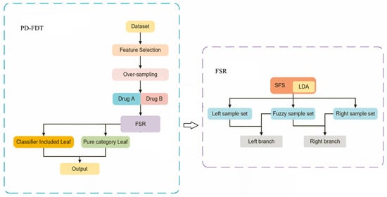
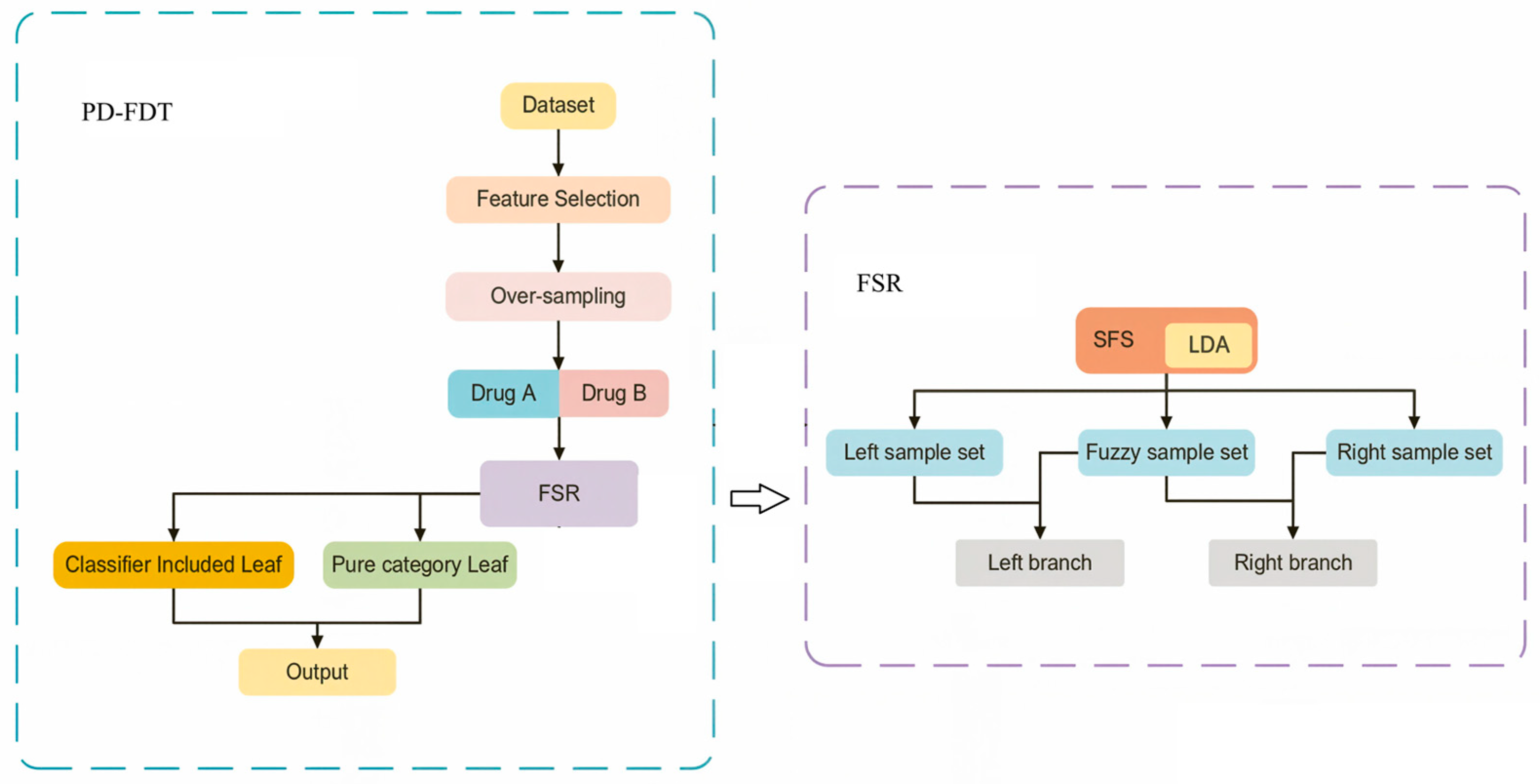
This section introduces the detailed procedure of the Drug Pair-based Fuzzy Decision Tree (DP-FDT) for improving the performance of drug combination, and the workflow chart of our algorithm is illustrated in Figure 1. It primarily illustrates the workflow of the PD-FDT. The process is divided into two main phases: the general pipeline of tree growth is shown on the left, and the detailed logic of the Fuzzy Split Rule (FSR) algorithm for the branch splitting of the tree is shown on the right.

Figure 1. Workflow chart of our algorithm.

Phase 1: The tree growth process. The workflow initiates with a raw dataset, which undergoes feature selection to identify the most relevant feature pairs. This is followed by oversampling to correct class imbalances in the data. The processed data is then separated into inputs for DrugA and DrugB, indicating that the model evaluates pairwise relationships between two pharmaceutical compounds. In the branch splitting process, it calls on the FSR algorithm to build each non-leaf node to grow the fuzzy decision tree.

Phase 2: The FSR module, as detailed on the right-hand side of the figure. It utilizes SFS (Sequential Feature Selection) and LDA (Linear Discriminant Analysis) to process the drug feature pairs. Unlike standard binary decision trees, the FSR module splits the data into three distinct subsets: the left sample set (directed to the left branch), right sample set (directed to the right branch) and fuzzy sample set. The presence of the “fuzzy sample set” indicates the use of fuzzy logic, allowing data points to have partial membership in multiple branches rather than a strict, forced categorization.

Phase 3: Classification and output. The branching paths from the FSR lead to terminal nodes in the decision tree. The diagram distinguishes between two types of leaves: classifier included and pure. The pure category implies a definitive classification, while classifier included type suggests a more complex leaf that may house additional classification logic. Ultimately, these leaves culminate in the final output, providing the model’s prediction or classification result. In summary, the PD-FDT workflow is a robust machine learning pipeline that integrates feature selection, data balancing, and fuzzy decision tree logic for drug combination prediction.

Since the combinatorial effects of drugs may vary across different cell lines, we need to model the samples from each cell line separately to predict cell-line-specific synergistic drug combinations. Each sample in the dataset represents a pair of drugs in a specific cell line. To ensure that all drugs in the training data have complete drug-induced gene expression profile features, we removed those drugs with missing feature information. Finally, we selected two typical cell lines with the largest sample sizes to construct the dataset, namely the A375 melanoma cell line and the A549 lung cancer cell line. The synergy score for each sample in the dataset is obtained by averaging the synergy scores from replicate experiments.

2.1. Growth Rules of Trees

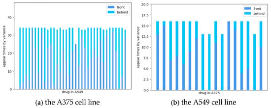
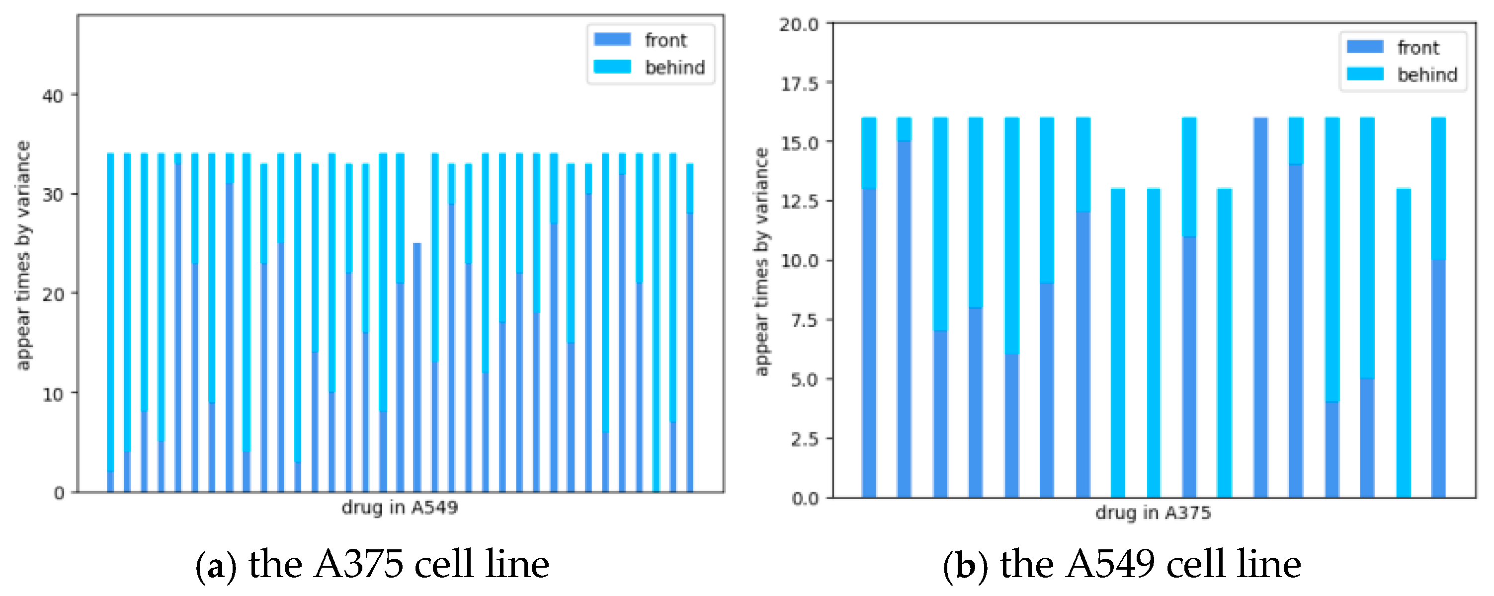
To handle the drug sequence problem, the drug combinations are divided into two sets based on the magnitude of their variances: one set contains the drugs with low variance in the combination, while the other set contains the drugs with high variance. This approach is used to determine the relative order of drugs in the dataset. Variance is used as the criterion to distinguish drugs because our statistical analysis has shown that the use of variance, mean, median, or other measures would lead to similar results. The distribution of the drugs is illustrated in Figure 2.

Figure 2. The variance distribution of the sequential relationship in different cell lines.

The general framework is given as Algorithm 1, calling the DP-FDT algorithm (given in Algorithm 2) to implement the main algorithm. And then DP-FDT calls on the GrowTree algorithm (given in Algorithm 3) to grow the tree iteratively. To handle a large number of features, firstly, the DP-FDT performs feature selection on the dataset. Since the algorithm takes into account the characteristics of drug combinations, it is necessary to select features in pairs during the feature selection process. Here, we use a feature selection method based on the chi-squared test to rank the importance of each feature and keep the top 50 feature pairs. Subsequently, we sum the ranks of each feature to obtain a new rank of feature pair importance by computing the average variance of feature pairs.

In this study, the raw features are Z-score-standardized and therefore contain negative values. Since the standard chi-square feature selection method is intended for non-negative variables, it cannot be applied directly to these continuous signed features. Therefore, instead of applying the standard chi-square test directly to the raw features, we first discretized each continuous Z-score feature into a small number of non-negative ordinal bins using training-fold-only equal-frequency discretization. We then applied the ordinary chi-square test of independence between the discretized feature and the class label.

Specifically, for each feature $f$ and each training fold, five bins are defined:

$$\begin{array}{c}\mathrm{b}\mathrm{i}\mathrm{n} 0:z<q_{20},\hfill \\ \mathrm{b}\mathrm{i}\mathrm{n} 1:q_{20}\le z<q_{40},\hfill \\ \mathrm{b}\mathrm{i}\mathrm{n} 2:q_{40}\le z<q_{60},\hfill \\ \mathrm{b}\mathrm{i}\mathrm{n} 3:q_{60}\le z<q_{80},\hfill \\ \mathrm{b}\mathrm{i}\mathrm{n} 4:z\ge q_{80}.\hfill \end{array}$$

(1)

Negative Z-scores are therefore handled naturally: strongly negative values fall into the lowest bin, and strongly positive values fall into the highest bin. If some quantile cut points are duplicated, we collapse adjacent bins to avoid empty categories. For feature $f$, build a $5\times C$ contingency table, where $C$ is the number of classes. In our datasets, $C=3$: antagonism, additive, and synergy. Let $O_{bc}$ be the observed count of samples in bin $b$ and class $c$, and let

$$E_{bc}={\displaystyle \frac{R_b{C}_c}{N}},$$

(2)

where $R_b={\sum }_c{O}_{bc}$, $C_c={\sum }_b{O}_{bc}$, and $N={\sum }_{b,c}{O}_{bc}$. Compute the chi-square statistic by

$${\chi }_f^2={\displaystyle {\sum }_{b=1}^5}{\displaystyle {\sum }_{c=1}^C}{\displaystyle \frac{{\left(O_{bc}-E_{bc}\right)}^2}{E_{bc}}}$$

(3)

A larger ${\chi }_f^2$ indicates stronger dependence between feature $f$ and the class label. We rank features by decreasing ${\chi }_f^2$. Ties are broken by average rank.

For the drug pair feature construction, let $r_A\left(i\right)$ be the chi-square rank of the $i$-th feature of DrugA and $r_B\left(i\right)$ the chi-square rank of the $i$-th feature of DrugB, where a rank of 1 represents the most important feature. For each corresponding feature pair $i$, we define the pair score:

$$R_i=r_A\left(i\right)+r_B\left(i\right).$$

(4)

We sort $R_i$ in ascending order and keep the top 50 feature pairs, as stated in Algorithm 1. The subsequent variance-based criterion then selects the top 30 pairs used for tree growth. Based on this new rank, the algorithm can then select the desired feature pair. Next, the algorithm applies oversampling using the Synthetic Minority Oversampling Technique (SMOTE) to the dataset, ensuring that the total weights of the classes remain consistent in the subsequent voting process. Then this algorithm selects the top 30 feature pairs of each sample and applies them to the related feature subsets F_A and F_B.

The pipeline is given as Algorithm 1. For each of the five outer folds $k=1,\dots ,5$. As the fraework of the algorithm, it calls Algorithm 2 to train DP-FDT model using the training data in each fold.

Algorithm 1. General Framework.

1. For each of the five outer folds $k=1,\dots ,5$: 2.    Split the full dataset into a training portion $D_{\mathrm{train}}^{\left(k\right)}$ and a held-out validation/test portion $D_{\mathrm{test}}^{\left(k\right)}$. The test portion is never used for any fitting. 3.    On $D_{\mathrm{train}}^{\left(k\right)}$ only: 4.         Discretize each continuous Z-score feature into five non-negative ordinal bins using equal-frequency cut points computed from $D_{\mathrm{train}}^{\left(k\right)}$; 5.         Compute the chi-square statistic for each feature and rank the features. 6.         Form feature pairs using $R_i=r_A\left(i\right)+r_B\left(i\right)$ where $r_A\left(i\right)$ and $r_B\left(i\right)$ are the chi-square ranks of the corresponding features of DrugA and DrugB. Keep the top 50 pairs. 7.         Compute the average variance of each drug pair on $D_{\mathrm{train}}^{\left(k\right)}$, determine the low/high variance ordering, and record the top 30 feature pairs in $F_A$ and $F_B$. 8.    Apply SMOTE only to $D_{\mathrm{train}}^{\left(k\right)}$ to obtain a balanced training set $D_{{train}^{\prime }}^{\left(k\right)}$. 9.    Train the DP-FDT model on $D_{{train}^{\prime }}^{\left(k\right)}$. 10.     Transform $D_{\mathrm{test}}^{\left(k\right)}$ using the same discretization cut points, selected feature pairs, and variance ordering learned from $D_{\mathrm{train}}^{\left(k\right)}$. No SMOTE is applied to $D_{\mathrm{test}}^{\left(k\right)}$. 11.     Predict on $D_{\mathrm{test}}^{\left(k\right)}$ and compute AUC, F1, recall, precision, and accuracy. 12. Repeat for all five folds and report the mean and standard deviation.

The tree growth process is shown in GrowTree (Algorithm 3). Assume the sample subset $S_k$ in node k (${node}_k$). Although the stop criterion is not satisfied, the algorithm would continue to grow the decision tree according to the rules described in GrowTree. The stop criterion includes the purity of $S_k$ and the sample size of $S_k$. If the size of $S_k$ is less than Θ, which is set to n/5, or the samples in $S_k$ belong to the same class, the node would not be split anymore. Only impure leaves are equipped with a logistic regression classifier; pure leaves directly output their class label. When a leaf node turns out to be impure upon termination of growth, a logistic regression classifier will be introduced to fit the samples, and the sample subsets in the left and right branches are represented as $S_k^l$ and $S_k^r$ respectively. Then, ${node}_k$ is set as an internal node with ${node}_k^{l,child}$ and ${node}_k^{r,child}$ as its left and right child nodes.

Algorithm 2. DP-FDT (D, Θ).

Input:  D: Training dataset (contains feature pairs for DrugA and DrugB);  Θ: Stop-growing threshold, set to |D|/5; Output:  T: A trained fuzzy decision tree;

1. // === Feature Selection (Chi-square) === 2. Compute the chi-square statistic for every individual feature pair; 3. Select the top 50 feature pairs with the highest chi-square scores;     (This forms the candidate pool for the next steps). 4. // === Data Balancing (SMOTE) === 5. Apply SMOTE to D to balance the class distribution, producing $D_{bal}$;     (Store the generated sample weights to ensure total class weights remain    consistent during later voting). 6. // === Variance Ranking === 7. For each feature pair i in the top-50 pool:     Compute the average variance of that feature pair across all samples in $D_{bal}$; 8. Rank the top-50 pairs in descending order of average variance; 9. Select the top 30 variance-ranked pairs; 10. Let $F_A$ = {indices of these 30 pairs for DrugA features}; 11. Let $F_B$ = {indices of these 30 pairs for DrugB features}; 12. // === Build the Tree === 13. Initialize the root node k with sample set $S_k$ = $D_{bal}$; 14. Return GrowTree($S_k$, $F_A$, $F_B$, Θ).

Algorithm 3. GrowTree (Recursive Node Splitting)

Input:  $S_k$: Sample subset at current ${node}_k$;  $F_A$ and $F_B$: Set of selected feature indices for DrugA and DrugB respectively (size 30);  Θ: Threshold for minimum sample size; Output:  ${sub\_tree}_k$: A trained subtree rooted at node k;

1. // Stop Criterion 1: Purity 2. If all samples in $S_k$ belong to the same class c:       Set ${node}_k$ as a leaf node labeled with class c;       Return ${sub\_tree}_k={node}_k$;   End if 3. // Stop Criterion 2: Sample size 4. If $‖S_k‖$< Θ:      Set ${node}_k$ as a leaf node, and label samples in $S_k$ as the label of the majority class;      Train a Logistic Regression classifier on all samples in $S_k$;      Attach the trained classifier to ${node}_k$;      Return ${sub\_tree}_k={node}_k$;   End if 5. // Otherwise, split the node using fuzzy rules 6. ($S_k^l$, $S_k^r$) = FSR($S_k$, $F_A$, $F_B$) // Fuzzy split (may produce overlapping subsets) 7. // Recursively grow left and right branches 8. ${node}_k^{l,child}$ = GrowTree($S_k^l$, $F_A$, $F_B$, Θ) 9. ${node}_k^{r,child}$ = GrowTree($S_k^r$, $F_A$, $F_B$, Θ) 10. Set ${node}_k$ as an internal node with ${node}_k^{l,child}$ and ${node}_k^{r,child}$ as its child nodes. 11. Return ${sub\_tree}_k=\left({node}_k^{l,child}\mathrm{a}\mathrm{n}\mathrm{d}{node}_k^{r,child}\right)$;

2.2. Fuzzy Splitting Rules for Trees

The scheme for splitting samples is implemented in Algorithm 4 Fuzzy Split Rules.

The split quality is calculated as follows: For a node sample set $S_k$, define

$$Gini\left(S_k\right)=1-{\displaystyle {\sum }_c}{p}_c^2$$

(5)

where $p_c$ is the proportion of samples in class $c$. For any candidate feature set $F$ and threshold $t$, after applying LDA we obtain a one-dimensional projection $z=\mathrm{L}\mathrm{D}\mathrm{A}\left(F\right)$. The weighted Gini impurity of the induced split is

$$G_{\mathrm{split}}\left(S_k;F;t\right)={\displaystyle \frac{\mid S_{k,L}\mid }{\mid S_k\mid }}Gini\left(S_{k,L}\right)+{\displaystyle \frac{\mid S_{k,R}\mid }{\mid S_k\mid }}Gini\left(S_{k,R}\right)$$

(6)

where $S_{k,L}=\left\{s\in S_k:z_s\le t\right\},S_{k,R}=\left\{s\in S_k:z_s>t\right\}.$ The best split quality for feature set $F$ is then

$$J\left(F\right)=\underset{t}{\mathrm{m}\mathrm{i}\mathrm{n}}{G}_{\mathrm{split}}\left(S_k;F;t\right)$$

(7)

In our algorithm, first, an empty candidate feature set ${\mathit{F}}^{\mathbf{*}}$ is initialized. All feature pairs are checked sequentially by combining each pair with the features in ${\mathit{F}}^{\mathbf{*}}$, using Linear Discriminant Analysis (LDA) to map them to one feature, based on whose Gini index the optimal split point is determined. To obtain the optimal t, each sample $s\in S_k$ is mapped to a one-dimensional score:

$$z_s={\mathrm{L}\mathrm{D}\mathrm{A}}_F\left(x_s\right)$$

(8)

where $x_s$ is the feature vector formed by $F$. Then, we sort all $z_s$ values in ascending order:

$$z_{\left(1\right)}\le z_{\left(2\right)}\le \cdots \le z_{\left(n\right)}$$

(9)

Only thresholds between consecutive distinct values can change the partition. So, for each $j=1,\dots ,n-1$ with $z_{\left(j\right)}<z_{\left(j+1\right)}$, consider

$$t_j={\displaystyle \frac{z_{\left(j\right)}+z_{\left(j+1\right)}}{2}}$$

(10)

If many values are tied, skip redundant midpoints. For each $t_j$, split the node into

$$G_{\mathrm{split}}\left(S_k;F;t_j\right)={\displaystyle \frac{\mid S_{k,L}\mid }{\mid S_k\mid }}Gini\left(S_{k,L}\right)+{\displaystyle \frac{\mid S_{k,R}\mid }{\mid S_k\mid }}Gini\left(S_{k,R}\right)$$

(11)

In this case, the best threshold is calculated using

$$t^{*}=\underset{t_j}{\mathrm{a}\mathit{rg}\min }{G}_{\mathrm{split}}\left(S_k;F;t_j\right)$$

(12)

The corresponding split quality is

$$J\left(F\right)=G_{\mathrm{split}}\left(S;F;t^{*}\right)$$

(13)

Then, the sum of the Gini indices of each feature pair is compared, and the feature pair with the smallest value is selected to insert to ${\mathit{F}}^{\mathbf{*}}$. This process is repeated until the performance can no longer be improved. It should be noted that if several thresholds give the same minimum Gini, the best parameter $t_j$ with two balanced child branches are selected to achieve the optimal splitting.

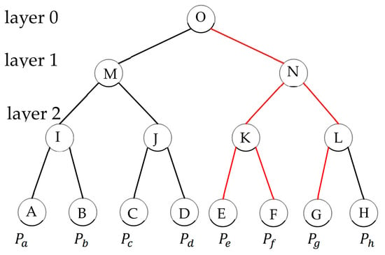
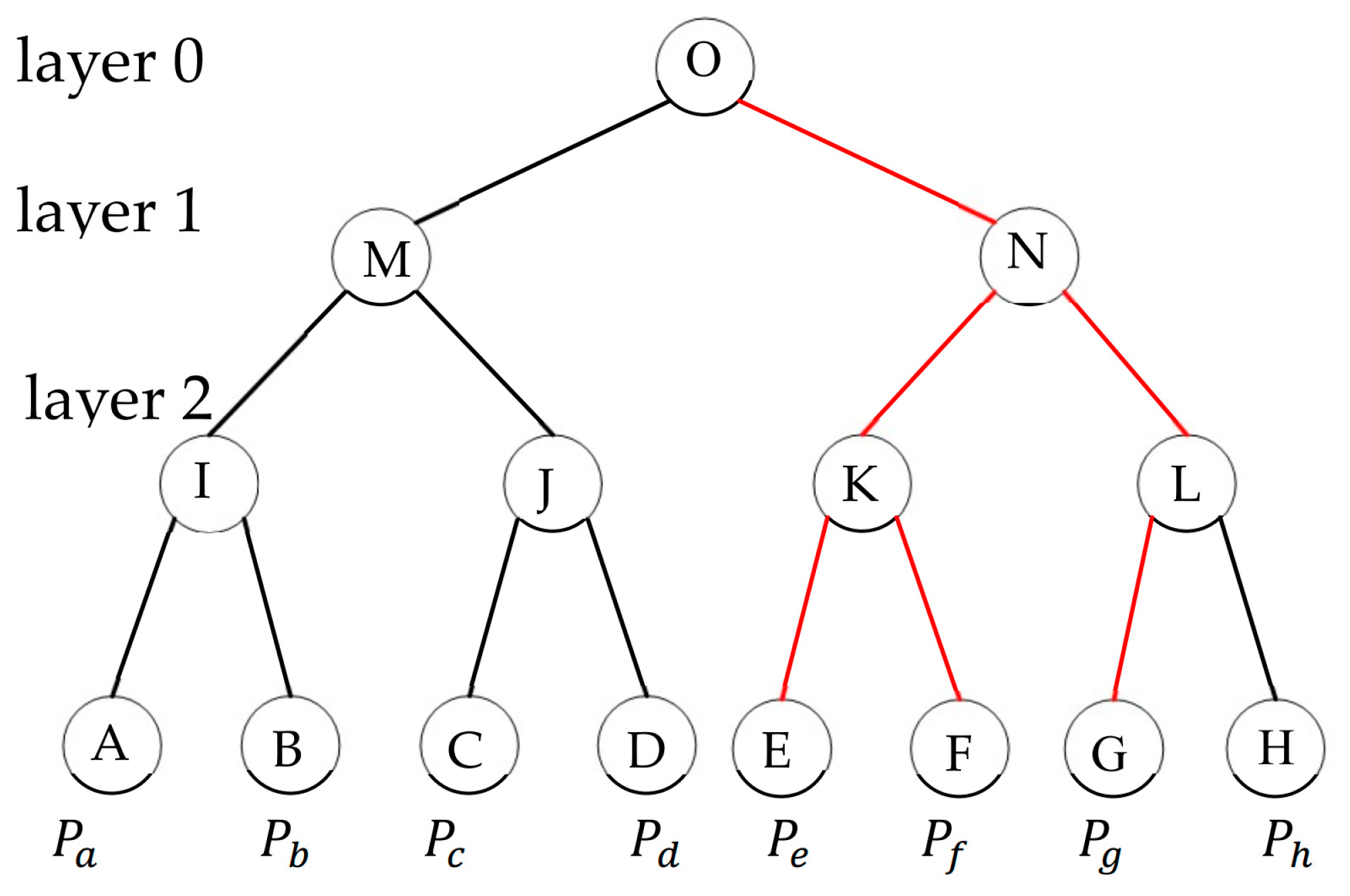
Finally, according to ${\mathit{F}}^{\mathbf{*}}$, both the left and right branches are partitioned by the sample subset of the node. For the i-th sample, the feature subset of DrugA and DrugB ($F_A^i$ and $F_B^i$) are deployed for each sample independently. If both $F_A^i$ and $F_B^i$, assign the i-th sample to the left/right branch; then, the sample would be sent to the left/right branch without uncertainty. However, if one feature subset assigns the sample to the right branch while the other assigns it to the left branch, the sample is treated as a fuzzy sample and is included in both the left and right branches simultaneously. In this case, it has a membership degree of 50% in each branch. This membership degree is used as the weight of the corresponding prediction. That is, during prediction, if an unknown sample enters both branches at a particular node, the voting weight along that path is split in half.

The final output is determined by multiplying the estimated probabilities of the related leaf nodes by their respective voting weights. An example is shown in Figure 3. Assume that the red path is the decision path taken by the $j$-th sample. Note that this sample is a fuzzy sample, as it is assigned simultaneously to nodes K and L at layer 2. So, its membership degree is 50% of nodes K and L respectively. It is then further assigned to leaf nodes E and F, which split from node K, and to leaf node G, which grows from node L. Consequently, its membership degree for E and F is reduced by 50%, so the weights for the predictions of both E and F are 0.25, while the weight for the prediction of G becomes 0.5. Thus, the final output combines the outputs of the three leaf nodes, E, F, and G. Consequently, the prediction for sample $j$ is calculated as ${\mathrm{Prob}}_j=0.5\times P_g+0.25\times P_f+0.25\times P_e$, where $P_g$, $P_f$, and $P_e$ represent the prediction probabilities associated with the corresponding leaf nodes, respectively.

Figure 3. An example of the prediction of the j-th sample in the DP-FDT.

Every accepted split strictly reduces the effective weighted sample size in each nonempty child relative to its parent. The recursion continues splitting until the stopping criterion is met: either $\mid S_k\mid <n/5$ or the node is pure. Consequently, any node whose sample size falls below $n/5$ becomes a leaf, which prevents excessive depth in practice. These conditions guarantee termination and prevent infinite recursion.

Algorithm 4. Algorithm Fuzzy Split Rules (FSR).

Input:  $S_k$: Sample subset at current ${node}_k$;  $F_A$ and $F_B$: Set of selected feature indices for DrugA and DrugB respectively (size 30); Output:  $S_k^l$ and $S_k^r$: Sample subset assigned to the left and right branches respectively;

1. // === Initialization === 2. ${\mathit{F}}^{\mathbf{*}}$ = ∅;  // Candidate feature set (indices) for this node 3. ${Previous}_{gini}$ = 0  // Track the best Gini impurity achieved 4. ${best\_split}_A$ = NULL, ${best\_split}_B$ = NULL; 5. // === Iteratively select feature pairs until no improvement === 6. While True:     ${best}_i$ = −1;     ${best}_{gini\_sum}$ = $+\infty$;     // --- Step A: Find the best candidate pair using sum of individual Ginis --- 7.    For i = 1 to v:         ${\mathit{F}}^{\mathit{t}\mathit{m}\mathit{p}}=\{F_A^i$$, F_B^i\} \cup$ ${\mathit{F}}^{\mathbf{*}}$         // (1) Evaluate Drug feature pairs;         $f_{tmp}$ = LDA(${\mathit{F}}^{\mathit{t}\mathit{m}\mathit{p}}$ in $S_k$); // Project ${\mathit{F}}^{\mathit{t}\mathit{m}\mathit{p}}$ to 1D using LDA;         Find $t^{*}$ to minimize Gini index by Formula (13);         Divide $S_k$ into two branches by $t^{*}$;         Calculate the Gini index on this node $P_i$: ${Gini}_{P_i}={Gini}_{F_A^i}$$+ {Gini}_{F_B^i}$;         If ${Gini}_{P_i}$$<{ best}_{gini\_sum}$:            ${best}_{gini\_sum}$$={Gini}_{P_i}$;            ${best}_i$ = i;         End for     // --- Step B: Test if adding ‘${best}_i$’ to F* improves the overall node split --- 8.    ${\mathit{F}}^{\mathit{t}\mathit{m}\mathit{p}}=\{F_A^{{best}_i}$$, F_B^{{best}_i}\} \cup$ ${\mathit{F}}^{\mathbf{*}}$;     // Evaluate the split quality using this combined projection     $J\left({\mathit{F}}^{\mathit{t}\mathit{m}\mathit{p}}\right)$ = OptimalSplitGini(${\mathit{F}}^{\mathit{t}\mathit{m}\mathit{p}}$)     // --- Step C: Performance check (Stop if no improvement) --- 9.    If $J\left({\mathit{F}}^{\mathit{t}\mathit{m}\mathit{p}}\right)$ > ${Previous}_{gini}$:        // Improvement achieved: commit the new pair        ${Previous}_{gini}$ = $J\left({\mathit{F}}^{\mathit{t}\mathit{m}\mathit{p}}\right)$;        ${\mathit{F}}^{\mathbf{*}}$ = ${\mathit{F}}^{\mathit{t}\mathit{m}\mathit{p}}$;     Else:        // No improvement: stop the loop        Break;       End If    End While 10. // === Finalize fuzzy splits using the selected F* === 11. Let $F_A^{selected}$ and $F_B^{selected}$ represented the selected features of DrugA and B in ${\mathit{F}}^{\mathbf{*}}$; 12. $f_A^{proj}=LDA$$(F_A^{selected}$); // Set a boundary using LDA with the selected features of Drug A; 13. $S_A^l$$= \{s\in S_k\left|f_A^{proj}\left(s\right)\le \right.T_A$}; // $T_A$ represents the threshold determined by LDA using Drug A; 14. $S_A^{r }$$= \{s\in S_k\left|f_A^{proj}\left(s\right)>\right.T_A$}; 15. $f_B^{proj}=LDA$$(F_B^{selected}$); // Set a boundary using LDA with the selected features of DrugB; 16. $S_B^l$ = $\{s\in S_k\left|f_B^{proj}\left(s\right)\le \right.T_B$}; //$T_B$ represents the Class Boundary determined by LDA using DrugB; 17. $S_B^r$ = $\{s\in S_k\left|f_B^{proj}\left(s\right)>\right.T_B$}; 18. Set the sample subset in the left branch $S_k^l$, where ${S_k^l=S_k-S}_A^r\cap S_B^r$; 19. Set the sample subset in the right branch $S_k^r$, where ${S_k^r=S_k-S}_A^l\cap S_B^l$; 20. Return the sample split scheme $S_k^l$ and $S_k^r$;

2.3. The Method for Result Analysis

Gene Ontology (GO) biological process enrichment dot plots are significant because they translate a list of genes into interpretable biological themes. They reveal which biological processes are over-represented among genes of interest and provide a visual summary of both statistical and biological importance.

To perform Gene Ontology (GO) biological process enrichment analysis, a gene list of interest (e.g., differentially expressed genes) and a background set comprising all genes that could have been detected in the experiment were first defined. Both the input genes and the background genes were mapped to GO biological process terms using a curated annotation source. For each GO biological process term, the number of input genes annotated to that term was counted; this value was designated as the Count. The GeneRatio was calculated as the Count divided by the total number of input genes with GO annotations. Under the null hypothesis, the expected proportion of input genes annotated to the term was defined as the number of background genes annotated to that term divided by the total number of background genes with GO annotations.

A hypergeometric test or a one-sided Fisher’s exact test was used to assess whether the observed Count was greater than expected by chance, yielding a raw p-value for each term. Because many terms were tested simultaneously, p-values were adjusted for multiple comparisons using a false discovery rate procedure, such as the Benjamini–Hochberg method. Terms were filtered using an adjusted p-value threshold (e.g., p < 0.05) and, optionally, a minimum Count or GeneRatio.

For visualization, a dot plot was constructed. GeneRatio was plotted on the x-axis and GO biological process term names on the y-axis. Count was represented by dot size, so that larger dots indicated more input genes annotated to the term. The adjusted p-value was represented by dot color, using a gradient from one color for highly significant terms to another for less significant terms. Terms were ordered by adjusted p-value or GeneRatio, and the top enriched terms were displayed. This plot reveals which biological processes are significantly over-represented in the input gene list.

3. Results

3.1. Experiment Settings

Our dataset is obtained from DrugComb (v1.4) [8], which consists of four types of synergy scores: Bliss Independence (Bliss), Highest Single Agent (HSA), Loewe Additivity (Loewe), and Zero Interaction Potency (ZIP). For these scores, positive values indicate that a drug combination is synergistic, while negative values indicate antagonistic effects. By integrating the four scores, each sample can be classified into one of three category labels: synergistic, antagonistic, and additive. Synergistic and antagonistic samples are defined as those for which all four synergy scores are positive or negative, respectively, while the remaining samples are classified as additive.

The DrugComb database includes the L1000 project from the LINCS database, which contains cell-line-specific drug-induced gene expression data. This project provides expression levels of 978 landmark genes under different perturbations and control conditions across various human cell lines. It was pointed out that the 978 landmark genes cover approximately 80% of the information contained in the full transcriptome of 12,328 genes [33].

Therefore, we first obtained Level 5 data of gene expression profile Z-scores from the L1000 project, which feature multi-dose and multiple compound stimulations, where each score represents the relative value of gene expression levels under drug perturbation. We extracted the unique gene expression profile for each drug using the MODZ method, which derives consensus replicate signatures from Level 4 data of the L1000 project. Then, the Z-scores were weighted and averaged based on Spearman correlation. Finally, using the 978-dimensional gene expression profiles generated by drug perturbations in different cell lines, we constructed the feature representation for each DrugBy concatenating the features of the two drugs into a single data entry, resulting in a 1956-dimensional feature vector [13]. The high feature dimensionality is a common issue in drug combination datasets, which may increase the complexity of data processing and affect the predictive performance of the model. In addition, Table 2 lists the sample counts for each class within each cell line. It can be seen that the number of samples labeled as additives is greater than the sum of the other two classes, indicating that the class distribution in the dataset is imbalanced, which also affects model training and prediction. It can be found that class imbalance and high-dimensional features are the two main problems present in these datasets. Our algorithm provides appropriate solutions to these issues.

Table 2. The details about the drug combination datasets.

Name	Sample Size	Feature Set Size	Sample Sizes of Different Classes
			Antagonistic	Additive	Synergy
A375	130	1956	21	74	35
A549	586	1956	168	347	71

3.2. Performance Comparison of Different Algorithms

In this subsection, we verify the performance of our algorithm on imbalanced datasets by comparing its performance with that of various other algorithms. We select OC1, CO2, WODT, HHCART, RandCART, DT GINI, DT ID3, DeepSynergy, CPDT and NEDT. (DT ID3/GINI are provided by the Scikit-learn toolbox. The other source codes are available online as listed below: OC1, RandCART, HHCART, CO2: https://github.com/maoqiangqiang/DecisionTreeBaseline (accessed on 27 September 2026); CPDT: https://github.com/MLDMXM2017/CPDT (accessed on 27 September 2026); NEDT: https://github.com/MLDMXM2017/NEDT (accessed on 27 September 2026); DeepSynergy: https://github.com/sujaykumarmag/DSP (accessed on 27 September 2026); and WODT: https://www.lamda.nju.edu.cn/code_WODT.ashx (accessed on 27 September 2026)). Models based on oblique decision trees as the primary comparison algorithms, along with the relatively simple deep-learning algorithm DeepSynergy. Because the sample size is not large, in many cases, the parameter tuning process would lead to overfitting. Therefore, we only use the default parameter settings in the comparisons. In addition, DeepSynergy is adjusted by setting the output layer to contain three nodes to fit the three-class problem.

The main evaluation metrics, AUC, F1 score, recall, and precision, are used because they can effectively capture both synergistic and antagonistic features.

It should be noted that these metrices are originally defined for the binary classification (ranking one positive class against one negative class); there is no single raw formula for the three-class problem. To evaluate a three-class model, we must extend AUC using aggregation strategies.

In a binary confusion matrix, we have four core components: TP (True Positives), FP (False Positives), TN (True Negatives), and FN (False Negatives). While TN is essential for calculating specificity and accuracy, it is mathematically absent from the denominators of precision and recall. When extending to three classes, we use the One-vs-Rest (OvR) strategy. For each class, we define its own TP, FP, and FN by treating the other two classes as the single negative group. TN exists but is ignored in these formulas. In this way, precision measures the exactness of positive predictions using Formula (5):

$$\mathrm{Precision}={\displaystyle \frac{TP}{TP+FP}}$$

(14)

Recall measures the completeness of capturing actual positives:

$$\mathrm{Recall}={\displaystyle \frac{TP}{TP+FN}}$$

(15)

Since recall and precision are often conflicting metrics, the F1 score is typically used as the primary evaluation metric. The Macro F1 (${F1}_{\mathrm{M}\mathrm{a}\mathrm{c}\mathrm{r}\mathrm{o}}$) score is the unweighted arithmetic mean of the F1 scores calculated for each individual class. For class i, let $F{1}_i$ be calculated by

$$F{1}_i=2\times {\displaystyle \frac{{Precision}_i\times {Reall}_i}{{Precision}_i+{Reall}_i}}$$

(16)

Let $N$ denote the total number of classes. It treats all classes equally, regardless of their sample size, as shown in Formula (8).

$${F1}_{\mathrm{M}\mathrm{a}\mathrm{c}\mathrm{r}\mathrm{o}}={\displaystyle \frac{1}{N}}{\sum }_{i=1}^{N}F{1}_i$$

(17)

A high ${F1}_{\mathrm{M}\mathrm{a}\mathrm{c}\mathrm{r}\mathrm{o}}$ score indicates that the model performs well across all classes, including the minority ones. It is highly sensitive to the model’s performance on the minority class, making it a preferred metric for imbalanced datasets.

In imbalanced classification, the ${F1}_{\mathrm{M}\mathrm{a}\mathrm{c}\mathrm{r}\mathrm{o}}$ score can be misleadingly high if the model simply predicts the majority class. So, the minority F1 ($F{1}_{minority}$) is a critical metric because it directly evaluates the model’s ability to correctly identify the rare but often most important cases, as shown in Formula (5). ${F1}_{\mathrm{M}\mathrm{i}\mathrm{n}\mathrm{o}\mathrm{r}\mathrm{i}\mathrm{t}\mathrm{y}}$ refers to the F1 score calculated specifically for the minority class, as the harmonic mean of the precision and recall of the minority class. Because there are two minority classes in the datasets, antagonism and synergy, the reported $F{1}_{minority}$ is calculated by

$$F{1}_{minority}={\displaystyle \frac{F{1}_{\mathrm{Antagonism}}+F{1}_{\mathrm{Synergy}}}{2}}$$

(18)

In summary, ${F1}_{\mathrm{M}\mathrm{a}\mathrm{c}\mathrm{r}\mathrm{o}}$ averages performance across all classes by computing each class’s F1 score, whereas $F{1}_{minority}$ reports the average F1 score of the antagonism and synergy classes, specifically to monitor whether the model is ignoring hard-to-detect subgroups.

In the similar One-VS-Rest method, the AUC metric is also re-defined by treating each class as the positive group, and the other two classes are merged into a single negative group so as to compute a binary AUC, and then the average AUC score is calculated to provide the average probability that, for any given class, the model ranks a random instance of that class higher than a random instance of all other classes combined.

It is noted that decision trees have relatively few parameters, which is one of their advantages. In addition, given the small sample sizes of the datasets, we only use the average of five-fold cross-validation for performance evaluation instead of nested cross-validation or another tuning protocol. We deploy the stratified cross-validation scheme to split the dataset into five folds while preserving class proportions.

As shown in Table 3 and Table 4, the best results are marked in bold. It shows that our DP-FDT algorithm outperforms or matches other comparative algorithms in terms of two key metrics, AUC and F1 score, on both the A375 cell line and the A549 cell line drug combination datasets. In particular, on the AUC metric, compared with the strongest baseline, NEDT, the proposed method improves AUC by 1.46 and 0.88 percentage points on A375 and A549, respectively. It should be noted that NEDT is a neural network embedded decision tree, which has much higher computational resources and achieves good performance. Compared with the remaining baseline methods, the AUC improvements range from 3.1 to 5.3 percentage points.

Table 3. Performance comparisons on the A375 dataset.

A375	AUC	${\mathit{F}1}_{\mathbf{M}\mathbf{a}\mathbf{c}\mathbf{r}\mathbf{o}}$	$\mathit{F}{1}_{\mathit{m}\mathit{i}\mathit{n}\mathit{o}\mathit{r}\mathit{i}\mathit{t}\mathit{y}}$	Recall			Precision			Rank
				Additive	Antagonism	Synergy	Additive	Antagonism	Synergy
OC1	0.4826	0.3218	0.1918	0.6895	0.1143	0.2400	0.5381	0.1586	0.2600	5.5
CO2	0.5248	0.2418	0.0000	1.0000	0.0000	0.0000	0.5692	0.0000	0.0000	7.7
WODT	0.5642	0.4258	0.3862	0.5533	0.3429	0.3900	0.5821	0.3079	0.5086	2.8
HHCART	0.5032	0.3025	0.2213	0.4705	0.3143	0.1500	0.4842	0.2396	0.1833	7.6
RandCART	0.5358	0.3739	0.2899	0.5276	0.4571	0.2000	0.6126	0.3718	0.1471	4.5
DT GINI	0.5340	0.3330	0.2679	0.4305	0.3429	0.2500	0.5152	0.2756	0.2133	5.3
DT ID3	0.5153	0.3147	0.2550	0.4752	0.1714	0.3300	0.4720	0.1414	0.3778	5.8
DeepSynergy	0.5071	0.1989	0.1335	0.3467	0.1429	0.5450	0.3731	0.0500	0.1154	7.7
CPDT	0.5363	0.3371	0.3251	0.3725	0.2724	0.3211	0.4720	0.2414	0.3362	6.1
NEDT	0.6021	0.3892	0.3752	0.4607	0.3471	0.5520	0.5837	0.3521	0.5163	2.6
DP-FDT	0.6167	0.4245	0.3723	0.5248	0.3714	0.4900	0.6302	0.4250	0.2310	2.2

Table 4. Performance comparisons on the A549 dataset.

A549	AUC	${\mathit{F}1}_{\mathbf{M}\mathbf{a}\mathbf{c}\mathbf{r}\mathbf{o}}$	$\mathit{F}{1}_{\mathit{m}\mathit{i}\mathit{n}\mathit{o}\mathit{r}\mathit{i}\mathit{t}\mathit{y}}$	Recall			Precision			Rank
				Additive	Antagonism	Synergy	Additive	Antagonism	Synergy
OC1	0.5535	0.3508	0.187	0.8155	0.2553	0.0419	0.6111	0.3846	0.1200	5.8
CO2	0.5058	0.2479	0.0000	1.0000	0.0000	0.0000	0.5921	0.0000	0.0000	7.9
WODT	0.5534	0.3883	0.2685	0.6428	0.3275	0.1971	0.6239	0.3628	0.1875	3.8
HHCART	0.5409	0.3675	0.2425	0.6400	0.2923	0.1819	0.6162	0.3122	0.1845	5.6
RandCART	0.5193	0.3734	0.2566	0.6168	0.2930	0.2257	0.6191	0.3019	0.2060	4.6
DT GINI	0.5471	0.3827	0.2691	0.6282	0.3939	0.1276	0.6127	0.3959	0.1602	4.7
DT ID3	0.5474	0.3885	0.2959	0.6109	0.4171	0.1810	0.6156	0.4103	0.1756	4.3
DeepSynergy	0.5004	0.2038	0.0910	0.5800	0.2000	0.2267	0.4593	0.0581	0.0577	7.9
CPDT	0.4986	0.2598	0.2607	0.6301	0.2867	0.2706	0.5817	0.3261	0.1902	6.7
NEDT	0.5849	0.3893	0.3059	0.6788	0.3956	0.3911	0.6225	0.3468	0.1875	2.9
DP-FDT	0.5937	0.3984	0.3378	0.4990	0.4000	0.4400	0.6337	0.3600	0.2052	2.6

Moreover, our calculations reveal that our algorithm achieves a significantly higher F1 score even for the minority class, indicating that it is better able to identify samples from the minority class. The ranking results also show that the DP-FDT algorithm ranks higher than all other algorithms, which suggests that overall, our algorithm does not lag behind the other comparative algorithms in performance.

3.3. Impact of the Number of Feature Selections on the Minimum Number of Samples per Leaf

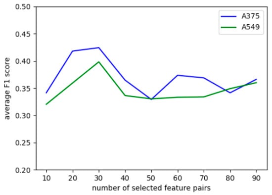
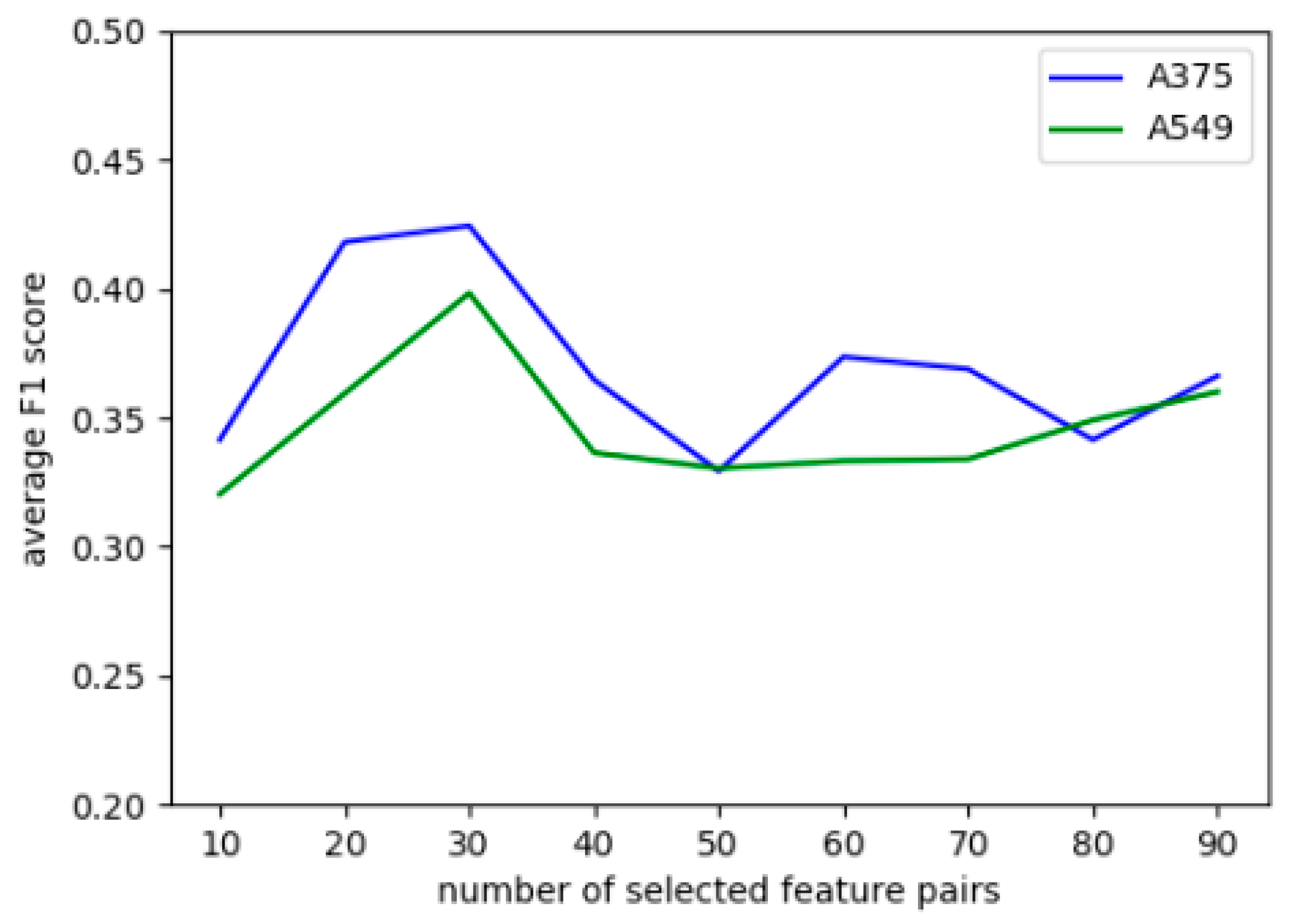
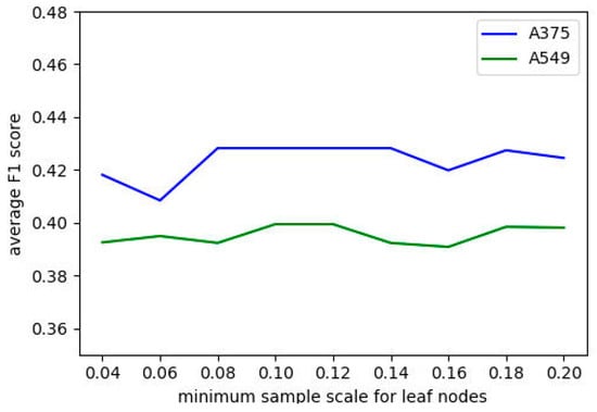
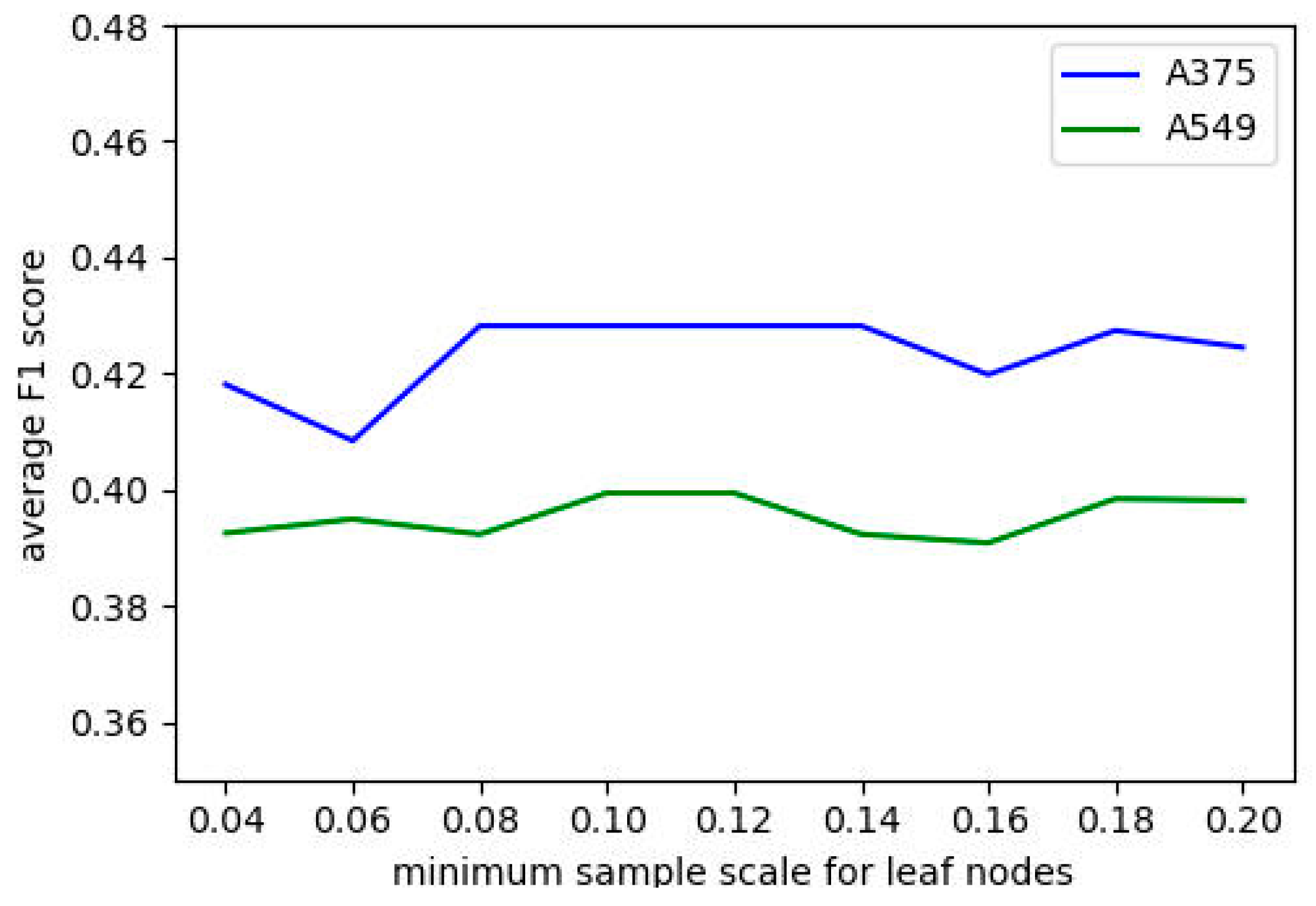
This section primarily discusses the impact of the number of feature pairs selected and the minimum number of samples per leaf node on the performance of the DP-FDT algorithm. The analysis is divided into two main experiments: In the first experiment, while keeping the minimum number of samples per leaf node constant, we varied the number of feature pairs selected and observed the trend in the average F1 score of the algorithm under five-fold cross-validation. The range of variation for the number of feature pairs selected was from 10 to 90. In the second experiment, while keeping the number of feature pairs constant, we varied the minimum number of samples per leaf node and observed the trend in the average F1 score of the algorithm under five-fold cross-validation. The ratio of the minimum number of samples per leaf node to the total number of samples ranged from 0.04 to 0.2. The results are shown in the figure below.

In Figure 4, as the number of selected feature pairs increases, ${F1}_{\mathrm{M}\mathrm{a}\mathrm{c}\mathrm{r}\mathrm{o}}$ first reaches a peak around 30 and then continues to fluctuate. Therefore, we can preliminarily conclude that selecting the top 30 feature pairs can ensure good algorithm performance while reducing computation time.

Figure 4. Average F1 score trend vs. number of selected feature pairs.

In Figure 5, as the minimum number of samples per leaf node increases, the F1 score does not exhibit any significant changes. Hence, we believe that under certain conditions, the minimum number of samples per leaf node is not directly correlated with performance. However, given the need to prevent overfitting of classifiers within leaf nodes and to minimize tree depth without compromising performance, we set the ratio of the minimum number of samples per leaf node to the total number of samples at 0.2.

Figure 5. Average F1 score trend vs. minimum samples in leaf nodes. It is confirmed. It is confirmed.

3.4. Ablation Study

In this section, we will evaluate the performance impact of different modules. Here, the six versions of our algorithm are set, as shown in Table 5.

Table 5. The different settings of six versions of our algorithm for ablation study.

v1	univariate without logistic regression and SMOTE.
v2	univariate without logistic regression.
v3	multivariate without logistic regression and SMOTE.
v4	multivariate without logistic regression.
v5	multivariate without SMOTE.
v6	multivariate logistic regression and SMOTE.

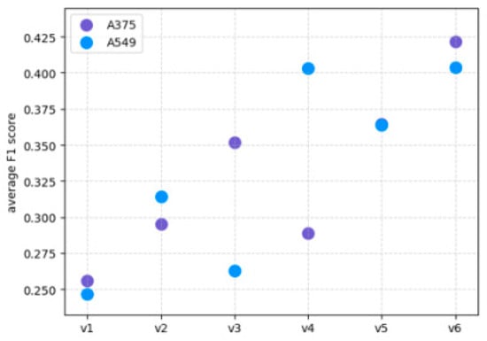
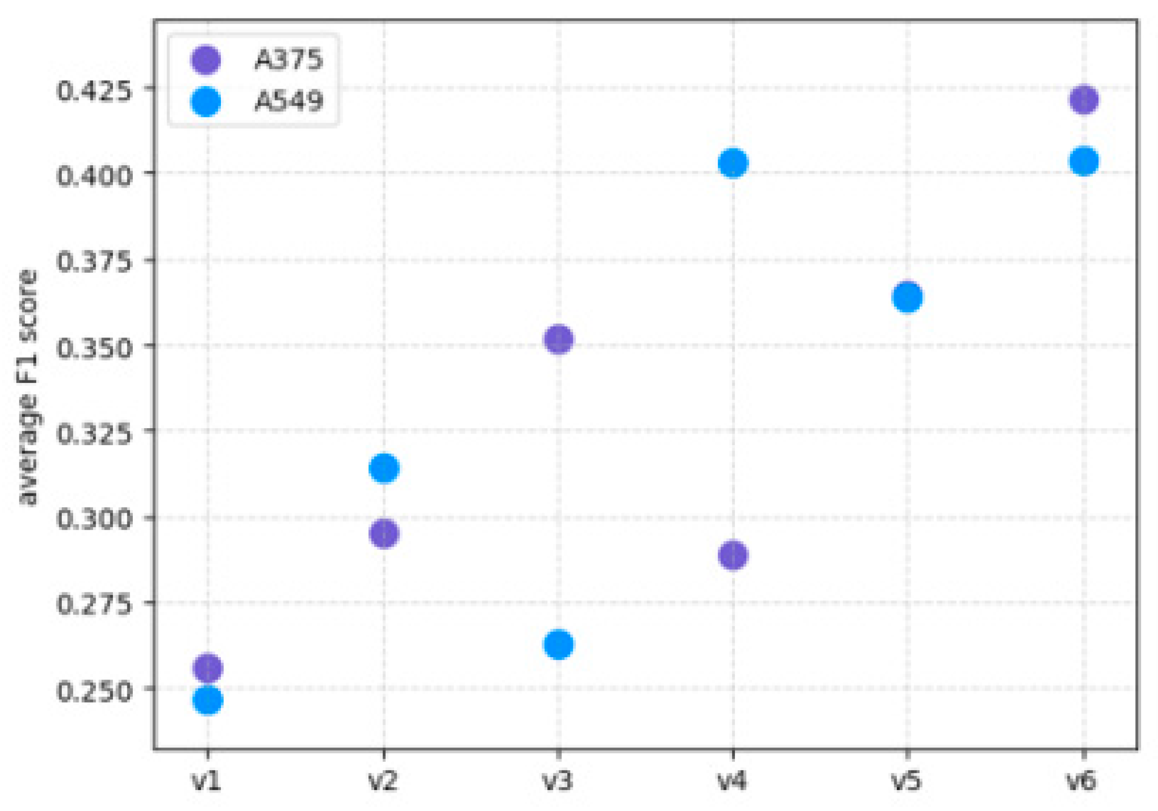
Among them, groups v1, v3, and v5 do not use the SMOTE oversampling algorithm to preprocess the dataset; in contrast, groups v2, v4, and v6 employ the SMOTE oversampling algorithm. Regarding the splitting rules for samples, groups v1 and v2 use a single feature pair to partition the data into left and right subtrees, whereas the remaining four groups use multiple feature pairs for splitting. As for the generation of leaf nodes, in the algorithms used by the first four groups, decision tree leaf nodes are not further subdivided using classifiers; in contrast, the last two groups apply a logistic regression classifier at the leaf nodes. Moreover, the final group represents the ultimate algorithm. Their performance, evaluated via five-fold cross-validation on two cell line datasets, is shown in Figure 6.

Figure 6. Impact of different modules on algorithm’s average F1 score across two datasets.

It can be seen that the algorithm’s performance increases linearly with the addition of modules, and the module combinations in the two control groups—v3 and v4—exhibit the greatest variability in performance across both datasets. This suggests that the logistic regression method used for leaf nodes, the SMOTE oversampling method, and the splitting rules for multi-feature pairs all have a significant impact on the algorithm’s performance. The abbreviations are as follows: vl, univariate without logistic regression and SMOTE; v2, univariate without logistic regression; v3, multivariate without logistic regression and SMOTE; v4, multivariate without logistic regression; v5, multivariate without SMOTE; v6, multivariate logistic regression and SMOTE.

3.5. Bioinformatics Analysis

To investigate the impact of drug-induced gene expression on synergistic effects, we selected key features that significantly influence the prediction process and further examined the genes involved in these key feature subgroups in this subsection.

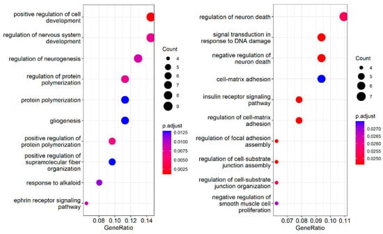
The two dot plots in Figure 7 present Gene Ontology (GO) biological process enrichment analyses for the A375 (left) and A549 (right) cell lines. In each plot, the y-axis lists enriched GO terms, while the x-axis shows GeneRatio, the proportion of input genes annotated to a given term. Dot size represents Count, the absolute number of genes associated with each term, and dot color represents the adjusted p-value. Redder dots indicate lower, more statistically significant p-values, whereas bluer dots indicate higher, less significant p-values. The analysis identifies biological processes over-represented in a gene list, likely differentially expressed genes.

Figure 7. GO biological process enrichment analysis on A375 (left) and A549 (right) cell lines.

The contribution of each feature to the prediction was determined by its selection frequency. On this basis, the top 134 features were identified for both the A375 and A549 cell lines. To characterize the genes associated with these contributing features, Gene Ontology (GO) biological process enrichment analysis was performed for the biological processes encoded by these features, with an adjusted p-value < 0.05, and the top 10 enriched results are shown in Figure 7.

For A375 melanoma cells (left panel), the most significant terms were related to development and neurobiology. These included positive regulation of cell development, regulation of nervous system development, regulation of neurogenesis, regulation of protein polymerization, protein polymerization, gliogenesis, positive regulation of protein polymerization, positive regulation of supramolecular fiber organization, response to alkaloid, and ephrin receptor signaling pathway. The top term, positive regulation of cell development, had the largest GeneRatio (approximately 0.14), a Count of 9, and the reddest color (adjusted p-value near 0.0025). This enrichment reflects the neural crest origin of melanocytes, from which melanoma arises, making the presence of neurogenesis, gliogenesis, and nervous system development terms biologically consistent. Additionally, protein polymerization and supramolecular fiber organization suggest active cytoskeletal remodeling, while ephrin receptor signaling is known to influence cancer cell migration and metastasis. Thus, A375 is characterized by developmental and neural lineage programs.

For A549 lung adenocarcinoma cells (right panel), the enriched terms shifted toward stress response, adhesion, and signaling. Key terms included regulation of neuron death, signal transduction in response to DNA damage, negative regulation of neuron death, cell–matrix adhesion, insulin receptor signaling pathway, regulation of cell–matrix adhesion, regulation of focal adhesion assembly, regulation of cell–substrate junction assembly, regulation of cell–substrate junction organization, and negative regulation of smooth muscle cell proliferation. The top term, regulation of neuron death, had a GeneRatio near 0.11, a Count of 7, and an adjusted p-value of around 0.025. The strong DNA damage response is typical of lung cancer and is often linked to carcinogen exposure and genomic instability. The cluster of cell–matrix and focal adhesion terms indicates epithelial–mesenchymal transition, invasion, and metastatic potential, while insulin receptor signaling is frequently dysregulated in lung cancer and associated with tumor progression. Neuron death terms may overlap with apoptotic and survival pathways that cancer cells exploit. Comparing the two cell lines, A375 showed enrichment for developmental and neural crest-derived programs, especially neurogenesis and gliogenesis, whereas A549 showed enrichment for DNA damage response, cell–matrix adhesion, focal adhesion assembly, and metabolic signaling. The color scales also differed: A375’s top terms reached lower adjusted p-values, indicating stronger statistical significance than A549’s top terms. Overall, the plots reveal distinct biological emphases consistent with the origins and phenotypes of melanoma and lung adenocarcinoma.

3.6. The Analysis on the Effect of Different Drug Order

To verify the contribution of our solution to the drug sequence, we compare a single random ordering of a drug pair’s feature subsets against our variance-based method (the scheme used in the algorithm). Table 6 shows that random ordering consistently degrades AUC, F1-macro, and F1-minority on both cell lines, whereas our method recovers the reported performance. This provides evidence that the beneficial effect of our method on the order comes from a more stable feature layout rather than from any biological ordering.

Table 6. Effect of the drug order assignment on DP-FDT.

Cell Line	Ordering Strategy	AUC	F1-Macro	F1-Minority
A375	Random order	0.5733	0.3629	0.3371
A375	Our method (Table 3)	0.6167	0.4245	0.3723
A549	Random order	0.5421	0.3673	0.2834
A549	Our method (Table 4)	0.5937	0.3984	0.3378

Table 7 reports the prediction agreement rate and the distribution of the gap when the two feature sets of a drug pair are swapped, i.e., |$P_{syn}\left(\mathrm{A}|\mathrm{B}\right)-P_{syn}\left(\mathrm{B}|\mathrm{A}\right)$|. The residual gap is small but non-zero, indicating that the model is not perfectly invariant to the order of the two drug feature subsets. Nonetheless, the high agreement rate and narrow gap distribution show that the proposed ordering largely stabilizes predictions, with only minor order-dependent effects remaining.

Table 7. Swap consistency of the fixed-order DP-FDT between (A|B) and (B|A).

Cell Line	Prediction Agreement Rate (%)	Mean |$∆{\mathit{P}}_{\mathit{s}\mathit{y}\mathit{n}}$|	Median |$∆{\mathit{P}}_{\mathit{s}\mathit{y}\mathit{n}}$|
A375	92.3	0.064	0.042
A549	90.2	0.075	0.049

Values for the fixed-order rows are taken directly from the DP-FDT entries of Table 3 (A375) and Table 4 (A549); the random-order rows are the new control and are pending final rounding of the rerun. $∆P_{syn}$ = |$P_{syn}\left(\mathrm{A}|\mathrm{B}\right)-P_{syn}\left(\mathrm{B}|\mathrm{A}\right)$| for the same trained fixed-order model. The agreement rate is the fraction of test pairs receiving the same predicted class under both orders.

4. Conclusions

This study proposed the Drug Pair-based Fuzzy Decision Tree (DP-FDT), an interpretable algorithm for drug combination prediction that directly addresses two major challenges in drug combination data: high-dimensional feature spaces and class imbalance. The DP-FDT incorporates drug combination feature pairs into feature selection and node construction, adopts fuzzy splitting rules so that samples can be assigned to multiple branches with certain probabilities, and attaches logistic regression classifiers to impure leaf nodes. These design choices improve fault tolerance, allow uncertain samples to be reconsidered, and enhance the model’s ability to identify minority-class samples.

Experimental results obtained on the A375 and A549 cell line datasets demonstrate that the DP-FDT achieves superior or competitive performance compared with several state-of-the-art oblique decision trees and a deep learning baseline, including OC1, CO2, WODT, HHCART, RandCART, DT-GINI, DT-ID3, DeepSynergy, CPDT, and NEDT. The DP-FDT consistently improves AUC and F1 scores, with AUC gains of up to 5.3 percentage points, and achieves higher minority-class F1 scores, indicating better detection of synergistic and antagonistic drug combinations that are often overlooked in imbalanced datasets. Ablation studies further confirm that SMOTE oversampling, multi-feature-pair splitting, and leaf-node logistic regression each make positive contributions to predictive performance.

Importantly, the bioinformatics analysis shows that the DP-FDT is not only a predictive model but also a tool for biological discovery. Based on feature selection frequency, the top 134 features were identified for each cell line and subjected to Gene Ontology biological process enrichment analysis. In A375 melanoma cells, the enriched processes were associated with neurogenesis, gliogenesis, nervous system development, protein polymerization, and ephrin receptor signaling, which are consistent with the neural crest origin of melanocytes and with active developmental and cytoskeletal programs in melanoma. In A549 lung adenocarcinoma cells, the enriched processes included DNA damage response, regulation of neuron death, cell–matrix adhesion, focal adhesion assembly, and insulin receptor signaling, reflecting stress adaptation, genomic instability, epithelial–mesenchymal transition, and invasive potential. These results connect the model’s internal feature importance to known cancer biology and demonstrate that the DP-FDT can generate biologically meaningful hypotheses.

Overall, the DP-FDT benefits the field of bioinformatics by providing an interpretable bridge between complex drug combination data and biological mechanisms. It enables researchers to identify feature pairs that contribute to synergy or antagonism, prioritize candidate gene expression signatures, and gain cell-line-specific insights into drug responses. The feature pair framework is also generalizable to other biomedical interaction prediction tasks involving paired entities, such as drug–target, protein–protein, or miRNA–disease interactions. In summary, the DP-FDT offers a practical and interpretable computational approach for drug combination prediction and bioinformatics analysis. Future work will focus on extending the method to more cell lines, integrating additional omics layers, and validating the identified biological processes through prospective experimental studies. In addition, although variance-based ordering improves stability, small order-dependent differences remain; future work could enforce permutation invariance more directly.

References

- Tan, Q.; Wen, Y.; Xu, Y.; Liu, K.; He, S.; Bo, X. Multi-view uncertainty deep forest: An innovative deep forest equipped with uncertainty estimation for drug-induced liver injury prediction. Inf. Sci. 2024, 667, 120342. [Google Scholar] [CrossRef] [Scilit]
- Wang, N.; Li, X.; Xiao, J.; Liu, S.; Cao, D. Data-driven toxicity prediction in drug discovery: Current status and future directions. Drug Discov. Today 2024, 29, 104195. [Google Scholar] [CrossRef] [Scilit] [PubMed]
- Zhang, W.; Xue, Z.; Li, Z.; Yin, H. DCE-DForest: A Deep Forest Model for the Prediction of Anticancer Drug Combination Effects. Comput. Math. Methods Med. 2022, 8693746. [Google Scholar] [CrossRef] [Scilit] [PubMed]
- Ye, Y.; Wen, Y.; Zhang, Z.; He, S.; Bo, X. Drug-Target Interaction Prediction Based on Adversarial Bayesian Personalized Ranking. BioMed Res. Int. 2021, 2021, 6690154. [Google Scholar] [CrossRef] [Scilit] [PubMed]
- Wang, W.; Guan, X.Q.; Khan, M.T.; Xiong, Y.; Wei, D.Q. LMI-DForest: A deep forest model towards the prediction of lncRNA-miRNA interactions. Comput. Biol. Chem. 2020, 89, 107406. [Google Scholar] [CrossRef] [Scilit] [PubMed]
- Kanehisa, M.; Furumichi, M.; Tanabe, M.; Sato, Y.; Morishima, K. KEGG: New perspectives on genomes, pathways, diseases and drugs. Nucleic Acids Res. 2017, 45, D353–D361. [Google Scholar] [CrossRef] [Scilit] [PubMed]
- Emmanuel, J.; Isewon, I.; Oyelade, J. An optimized deep-forest algorithm using a modified differential evolution optimization algorithm: A case of host-pathogen protein-protein interaction prediction. Comput. Struct. Biotechnol. J. 2025, 27, 595–611. [Google Scholar] [CrossRef] [Scilit] [PubMed]
- Bulat, Z.; Jehad, A.; Zheng, S.; Wang, W.; Wang, Y.; Joseph, S.; Alina, M.; Mohieddin, J.; Ziaurrehman, T.; Alberto, P. DrugComb: An integrative cancer drug combination data portal. Nucleic Acids Res. 2019, 47, W43–W51. [Google Scholar] [CrossRef] [Scilit] [PubMed]
- Tian, Y.; Yi, J.; Wang, N.; Wu, C.; Peng, J.; Liu, S.; Yang, G.; Cao, D. Ddinter 2.0: An enhanced drug interaction resource with expanded data coverage, new interaction types, and improved user interface. Nucleic Acids Res. 2025, 53, D1356–D1362. [Google Scholar] [CrossRef] [Scilit] [PubMed]
- Bender, A.; Thomas, M.C.; Scannell, J.W.; Shaywitz, D.A.; Ghiandoni, G.M.; Greener, J.G.; Pruteanu, L.-L.; Jacobson, R.D.; Handa, K.; Hirano, M.; et al. Artificial intelligence in drug discovery—what it is, where we stand and the path forward. Nat. Rev. Drug Discov. 2026. Online ahead of print. [Google Scholar] [CrossRef] [Scilit] [PubMed]
- Liu, W.; Lin, H.; Huang, L.; Peng, L.; Tang, T.; Zhao, Q.; Yang, L. Identification of miRNA-disease associations via deep forest ensemble learning based on autoencoder. Brief. Bioinform. 2022, 23, bbac104. [Google Scholar] [CrossRef] [Scilit] [PubMed]
- Ianevski, A.; Simonsen, R.M.; Myhre, V.; Tenson, T.; Oksenych, V.; Bjørås, M.; Kainov, D.E. DrugVirus. info 2.0: An integrative data portal for broad-spectrum antivirals (BSA) and BSA-containing drug combinations (BCCs). Nucleic Acids Res. 2022, 50, W272–W275. [Google Scholar] [CrossRef] [Scilit] [PubMed]
- Wu, L.; Wen, Y.; Leng, D.; Zhang, Q.; Dai, C.; Wang, Z.; Liu, Z.; Yan, B.; Zhang, Y.; Wang, J. Machine learning methods, databases and tools for drug combination prediction. Brief. Bioinform. 2022, 23, bbab355. [Google Scholar] [CrossRef] [Scilit] [PubMed]
- Preuer, K.; Lewis, R.P.I.; Hochreiter, S.; Bender, A.; Bulusu, K.C.; Klambauer, G. DeepSynergy: Predicting anti-cancer drug synergy with Deep Learning. Bioinformatics 2018, 34, 1538–1546. [Google Scholar] [CrossRef] [Scilit] [PubMed]
- Kuru, H.I.; Tastan, O.; Cicek, E. MatchMaker: A Deep Learning Framework for Drug Synergy Prediction. IEEE/ACM Trans. Comput. Biol. Bioinform. 2021, 19, 2334–2344. [Google Scholar] [CrossRef] [Scilit] [PubMed]
- Chen, X.; Ren, B.; Chen, M.; Wang, Q.; Zhang, L.; Yan, G. NLLSS: Predicting synergistic drug combinations based on semi-supervised learning. PLoS Comput. Biol. 2016, 12, e1004975. [Google Scholar] [CrossRef] [Scilit] [PubMed]
- Zhang, T.; Zhang, L.; Payne, P.R.; Li, F. Synergistic drug combination prediction by integrating multiomics data in deep learning models. Transl. Bioinform. Ther. Dev. 2021, 2194, 223–238. [Google Scholar] [CrossRef] [Scilit] [PubMed]
- Menden, M.P.; Wang, D.; Mason, M.J.; Szalai, B.; Bulusu, K.C.; Guan, Y.; Yu, T.; Kang, J.; Jeon, M.; Wolfinger, R.; et al. Community assessment to advance computational prediction of cancer drug combinations in a pharmacogenomic screen. Nat. Commun. 2019, 10, 2674. [Google Scholar] [CrossRef] [Scilit] [PubMed]
- Chen, J.; Wu, L.; Liu, K.; Xu, Y.; He, S.; Bo, X. EDST: A decision stump based ensemble algorithm for synergistic drug combination prediction. BMC Bioinform. 2023, 24, 325. [Google Scholar] [CrossRef] [Scilit] [PubMed]
- Wu, L.; Ye, X.; Zhang, Y.; Gao, J.; Lin, Z.; Sui, B.; Wen, Y.; Wu, Q.; Liu, K.; He, S. A genetic algorithm-based ensemble learning framework for drug combination prediction. J. Chem. Inf. Model. 2023, 63, 3941–3954. [Google Scholar] [CrossRef] [Scilit] [PubMed]
- Yan, B.; Ye, X.; Wang, J.; Han, J.; Wu, L.; He, S.; Liu, K.; Bo, X. An Algorithm Framework for Drug-Induced Liver Injury Prediction Based on Genetic Algorithm and Ensemble Learning. Molecules 2022, 27, 3112. [Google Scholar] [CrossRef] [Scilit] [PubMed]
- Lin, Z.; Chen, J.; Wu, L.; Liu, K.; Xu, Y.; He, S.; Bo, X. MOCT: A Multi-class Oblique Tree Algorithm for Synergistic Drug Combination Prediction. IEEE Trans. Comput. Biol. Bioinform. 2025, 23, 407–418. [Google Scholar] [CrossRef] [Scilit] [PubMed]
- Wu, L.L.; Gao, J.; Zhang, Y.X.; Sui, B.S.; Wen, Y.Q.; Wu, Q.Q.; Liu, K.H.; He, S.; Bo, X.C. A hybrid deep forest-based method for predicting synergistic drug combinations. Cell Rep. Methods 2023, 3, 100411. [Google Scholar] [CrossRef] [Scilit] [PubMed]
- Lin, Z.; Xu, Y.; Liu, K.; Chen, L. MDGP-forest: A novel deep forest for multi-class imbalanced learning based on multi-class disassembly and feature construction enhanced by genetic programming. Pattern Recognit. 2026, 170, 112070. [Google Scholar] [CrossRef] [Scilit]
- Chen, Y.; Zhang, Y.; Tan, Y. A comparative study of the cost–benefit strategy with the learning ensembles of decision stumps in polymetallic prospectivity modelling. Earth Sci. Inform. 2022, 15, 57–72. [Google Scholar] [CrossRef] [Scilit]
- Chen, S.; Wu, L.; Xu, Y.; Liu, K.; He, S.; Bo, X. A Multi-View Learning-Based Bayesian Ruleset Extraction Algorithm For Accurate Hepatotoxicity Prediction. In Proceedings of the 2023 IEEE International Conference on Bioinformatics and Biomedicine (BIBM); IEEE: Piscataway, NJ, USA, 2023; pp. 1054–1059. [Google Scholar]
- Landwehr, N.; Hall, M.; Frank, E. Logistic Model Trees. Mach. Learn. 2005, 59, 161–205. [Google Scholar] [CrossRef] [Scilit]
- Gama, J.; Brazdil, P. Cascade Generalization. Mach. Learn. 2000, 41, 315–343. [Google Scholar] [CrossRef] [Scilit]
- Seewald, A.K.; Petrak, J.; Widmer, G. Hybrid Decision Tree Learners with Alternative Leaf Classifiers: An Empirical Study. In Proceedings of the FLAIRS-01 Proceedings, Key West, FL, USA, 22–24 May 2000. [Google Scholar]
- Zou, J.; Wu, L.; Lin, W.; Liu, K.; Xu, Y.; He, S.; Bo, X. CPDT: A Novel Cluster-based Paired Decision Tree for Identifying Biomedical Entity Interactions. In Proceedings of the 2024 IEEE International Conference on Bioinformatics and Biomedicine (BIBM); IEEE: Piscataway, NJ, USA, 2024; pp. 3042–3047. [Google Scholar]
- Zou, J.; Wu, L.; Liu, K.; Xu, Y.; He, S.; Bo, X. A feature pair-based neural network embedded decision tree for synergistic drug combination prediction. Pattern Recognit. 2025, 164, 111608. [Google Scholar] [CrossRef] [Scilit]
- Chen, J. DC-FMDT: A Fuzzy Model Decision Tree Algorithm Based on Drug Combination Features. In Proceedings of the 2023 4th International Conference on Computer Engineering and Application (ICCEA), Hangzhou, China, 7–9 April 2023; pp. 400–405. [Google Scholar]
- Lamb, J.; Crawford, E.D.; Peck, D.; Modell, J.W.; Blat, I.C.; Wrobel, M.J.; Lerner, J.; Brunet, J.-P.; Subramanian, A.; Ross, K.N.; et al. The Connectivity Map: Using Gene-Expression Signatures to Connect Small Molecules, Genes, and Disease. Science 2006, 313, 1929. [Google Scholar] [CrossRef] [Scilit] [PubMed]
Disclaimer/Publisher’s Note: The statements, opinions and data contained in all publications are solely those of the individual author(s) and contributor(s) and not of MDPI and/or the editor(s). MDPI and/or the editor(s) disclaim responsibility for any injury to people or property resulting from any ideas, methods, instructions or products referred to in the content. |
© 2026 by the authors. Licensee MDPI, Basel, Switzerland. This article is an open access article distributed under the terms and conditions of the Creative Commons Attribution (CC BY) license.