


Abstract
We extend our description of the electron’s quaternion spin (Q–spin) as a geometric rotor. This follows from incorporating both the symmetric polarization and the antisymmetric coherence into the theory. Polarization is observed only through the local process we call contextual instantiation. For an EPR pair the observed correlation is reconstructed statistically from the coincidence populations and follows from the scalar invariant of the quaternion rotor, yielding the observed correlation. Numerical simulations reproduce this correlation using only local detector events, and show the same data retain complementary polarization and coherence structure producing a lemniscate rotor portrait. Because spin observables are not jointly definable on a single Kolmogorov probability space, the CHSH quadruple cannot be formed and Bell’s theorem is therefore not applicable. The results provide a unified geometric description of spin, measurement, and Bell correlations, contributing to the foundations of quantum mechanics.
1. Introduction
The fundamental conceptual problem with spin in standard quantum mechanics (QM) is that it is treated as an intrinsic property whose mathematical behaviour is well defined, while its underlying physical mechanism or geometric origin remains unexplained. In quantum field theory (QFT) [1], the fermion is taken as fundamental and represented mathematically by a vector in an abstract two–dimensional Hilbert space. Here we explore an alternative approach in which spin is treated as a bivector [2,3,4,5,6,7,8], rather than as a point-like carrier of abstract spin variables. The bivector geometry suggests that the bosonic bivector structure is fundamental with fermionic states emerging from the bivector dynamics. Throughout this paper, physical spin is represented by a quaternion rotor whose bivector component carries the geometric information responsible for polarization and coherence.
The Standard Model (SM) is formulated within the Clifford algebra [9,10], whereas the present approach employs the algebra . The distinction is both algebraic and ontological. We refer to this alternative approach as the Bivector Standard Model (BiSM) [5]. The two are fundamentally different and applicable in the high and low energy regimes we denote by HEP and LEP. Most notably quantum spin acquires a geometric origin as a classical bivector.
We find that bivector spin separates naturally into two distinct but complementary sectors describing states of opposite parity [2]. In isotropy, the magnetic state consists of the two blades of the bivector, 1 and 3, precessing about the 2 axis, shown on the left of Figure 1. The system balances constant external torque with internal dynamics and forms a conservative system. The quantum regime is reached when Euclidean (or Minkowski) space bifurcates into dual spaces of opposite parity [2]. Within the BiSM the even–parity sector is identified with matter, whereas the odd–parity sector is associated with force.
Figure 1.
Classical spin bifurcation. Left: The isotropic spin-1 bivector formed from the orthogonal blades 1 and 3 which precess about axis 2, directed out of the page. Center: The two mirror–related chiral states, , of opposite handedness, separated by the mirror plane bisecting the 1–3 axes. A spin-1 boson state forms along this direction. Right: When the two blades meet in their mirror plane, the left and right opposite precessions form the even-parity quantum state of pure mass. Reflection is lost, and the left and right states intertwine into a double helix.
The situation changes in a polarizing environment. There the isotropy of the state is replaced by an interaction that causes one blade of the bivector to align with the field, producing a polarized state denoted by . The other blade remains in high precession orthogonal to the polarized blade. The resulting structure appears as a vector carrying the familiar observable properties of the electron and interacting with an external field. In this case the electron carries two distinct domains: a polarized alignment and an internal coherence. Together these form a rotor.
This brings us to the distinction revealed by Bell inequalities (BI) [11]. The CHSH bound [12] applies to correlations constructed solely from Boolean outcomes . Such correlations are purely algebraic and contain no geometric contribution. The central observation of EPR experiments [12,13,14] is that the observed correlations violate this bound. We take the CHSH bound to mark the limit of the algebraic correlation Bell expressed, while the violation reflects additional geometric effects that naturally arise from the structure of the bivector.
The origin of the violation is long–range phase coherence shared by Alice and Bob [15,16,17]. This coherence is not visible in individual detection events. Rather it appears only after the data, recorded independently at remote stations, are brought together and analysed. Only then do variations in the coincidence populations reveal the underlying phase relation.
The purpose of this paper is to develop further the description of spin as a classical bivector [5]. First, we show how its geometric structure is essential to measurement. Second, when applied to the EPR paradox, we identify the long–range common phase that persists after separation. The bivector structure then provides a natural origin for the observed violation of the CHSH bound.
To motivate our approach we first present a physical and geometrical description of bivector spin and its associated phase coherence. Section 2 explains contextual instantiation and introduces the bivector basis for spin. Section 3 then formalizes these ideas mathematically and presents a geometrical basis for parity arising from mirror states. This Section continues by showing that the violation of BI arises because there is no single Kolmogorov probability space [18] on which Bell’s theorem can be constructed. Since the foundations of QM suffer from semantic ambiguities, we attempt to state the present approach as objectively as possible. Section 4 gives a simulation that maintains an EPR pair as a quaternion rotor up to detection. This is contrasted with Bell’s CHSH polytope from a Boolean description, and how the bivector introduces harmonics through its geometric structure. Section 5 suggests new experiments and discusses some consequences. This paper belongs to a line of research that developed after Fine’s theorem [19] in which BI become a more fundamental statement about joint probability. In Section 5.5 of Section 5 we review some of that post–Fine literature.
Section 3 questions Bell’s locality theorem [11,12,20] which states that no local realistic theory satisfying the CHSH inequality can reproduce the observed quantum correlations. The tension raised by Fine’s theorem [19] is that the inequalities [11,12] also require joint definability of the counterfactual variables. Failure of either locality or joint definability leads to failure of Bell’s locality theorem.
Assumption 1
(Bell–CHSH Structural Assumptions). The derivation of the CHSH inequality rests on the following premises:
- 1.
- Locality. The outcome at one wing is independent of the distant setting.
- 2.
- Outcome Definiteness. For each hidden parameter λ, the outcomesare well-defined elements of .
- 3.
- Joint Definability. The four counterfactual variablesare simultaneously defined measurable functions on a single Kolmogorov probability space .
Fine’s theorem transformed Bell’s theorem from locality into a precise mathematical statement, (3) in Assumption 1. Considerable literature followed, focusing on identifying the physical origin of the failure, why such a probability space should fail to exist, and on locating the obstruction within probability theory by introducing contextual or non–Boolean probability spaces, reviewed in Section 5.5. The present work accepts Fine’s characterization but does not challenge Bell’s derivation. Rather it takes BI as defining the algebraic limit upon which we build. In particular, we examine whether (3) in Assumption 1 accurately reflects the geometry of spin when spin is modeled as a real object with structure in . We argue that it does not. The four polarization observables required for the CHSH construction are not jointly definable and Fine’s theorem is therefore not applicable to bivector spin.
One aim of this paper is to make this point precise. We show that once the joint–definability premise is removed, the quaternion rotor structure of bivector spin directly yields the rotationally invariant correlation
without invoking nonlocality.
2. Bivector Spin
2.1. Bivector Spin and the Singlet State
Quaternion or Q-spin [2,5] is motivated by the geometric product of the Pauli components [9],
Definition 1
(Q-spin). Q-spin is a spin object possessing both vector and bivector sectors,
where the vector part describes polarization and the bivector part describes coherence. Together they constitute the quaternion rotor representing spin.
In the BiSM both terms are retained. Conventional QM [21] identifies the observable spin components with the vector contribution, , while the bivector contribution is not normally assigned an independent physical role. However, the two terms correspond to symmetric and antisymmetric contributions and both are required for a complete description of spin.
The bivector introduces an oriented plane so that spin possesses both an axis and the plane associated with that axis. Together they endow spin with a two–dimensional planar structure composed of two orthogonal angular–momentum components, thereby giving rise to the bivector shown on the left of Figure 1. The Body Fixed Frame (BFF) of the bivector is written as where the subscript s denotes spin spacetime. This BFF is oriented within the Laboratory Fixed Frame (LFF), which is Minkowski space written as .
Below we show [2] that the internal bivector state reduces to a simple quaternion rotor in the BFF,
where labels the internal rotor phase and I is a bivector satisfying . This state is isotropic, local, and undergoes only internal rotational motion. Unit quaternions satisfy Euler’s equation [9],
The scalar component of the rotor is expressed by the angled brackets,
and is Lorentz invariant [9]. The phase parameter is generated by the proper–time evolution of the rotor and is likewise Lorentz invariant.
In the BiSM long–range EPR correlation originates from a common relative rotor phase established at separation and subsequently carried along the worldlines of Alice and Bob. As shown later, the experimentally observed correlation is obtained from the scalar part of the corresponding rotor product yielding the familiar dependence.
This approach also introduces an associated local bivector field surrounding the bivector in . It is characterised by both phase and orientation. In our treatment, the Dirac equation motivates the structure of this bivector field. We emphasize that this local field is fundamentally different from the conventional Dirac field of QFT [1].
2.1.1. BiSM Singlet State
The two members of an EPR pair carry complementary states and whose product forms the identity operator in ,
The superscript “0” denotes the local singlet state before separation. Without the superscript denotes the identity of an EPR pair in free flight after separation. The singlet is represented as the product of two complementary rotor states whose combined geometry is isotropic. This expression does not represent the usual LFF singlet state but rather the isotropy of the BFF. No preferred polarization axis exists in this state. The identity operator arises from the exact compensation of the complementary rotor states. It characterizes the rotational symmetry of the pair prior to separation and persists after separation as a common phase relation shared by the two.
2.1.2. The Fermion Singlet
Conventionally [22] the singlet state is expressed as a pair of oppositely polarized fermions giving the view that the polarizations of Alice and Bob compensate one another. The two states represent the up/down polarization eigenstates of spin in a magnetic field. The isotropy of the singlet state is expressed as an entangled state,
State vectors such as Equation (10) do not explicitly display coherence. Taking the outer product gives the corresponding state operator [23],
The entanglement is reflected in the off–diagonal coherence terms contained within the scalar product. Pauli vector components are present. In contrast, the bivector singlet of Equation (9) is not entangled. It is devoid of vector components. Correlation instead originates from the common phase established at separation.
2.1.3. An EPR Pair in Free Flight
We assume locality throughout. As Alice and Bob separate from the isotropic singlet state they do so in opposite directions conserving linear momentum. Each particle carries two properties. One is its proper time . The other is a spatial phase . Both must also be conserved between the pair giving an overall phase,
For ideal coincidence pairing the proper times are matched. The two spatial phases are then also matched, apart from their anti–correlation, and they do not cancel after spatial separation nor do they decohere. Within the local singlet is not defined. It is created at separation and then carried independently by Alice and Bob. Figure 2 shows the two cases. The bound single in the center panel, changes to after separation, depicted by the left and right panels. They represent two physically distinct but correlated compensating rotors. The anti–correlated preparation is evident from .
Figure 2.
Spatial separation of an EPR pair. The center panel shows the initial singlet, , at the point of separation. The left and right panels are spatially, not temporally, separated to show the two rotors carried by Alice and Bob, each with common phase . The two together represent .
These phase parameters, once established, remain unchanged until interrupted by an interaction such as detection. Those events are recorded at Alice and Bob and added to their appropriate local bins, not as coincidences, but as single Boolean events recorded independently at each remote station. Clicks are collected for all filter settings a at Alice’s location and b at Bob’s location. Coincidences are extracted after the experiment terminates.
Although the EPR pairs propagate independently after separation, they continue to carry complementary rotor states originating from the same singlet preparation. The geometric relation between the two particles is,
where , with denoting the axis of linear momentum. We added the dots to emphasize that the two rotors do not cancel but are carried as independent phases by the separated EPR pair. The dots have no mathematical meaning expressing only locality by the product. Conserving internal angular momentum at separation requires a common phase . Since the two components are carried separately, the actual distance between Alice and Bob can be vast. This is the origin of the long–range phase coherence that we later argue is responsible for the violation of BI. Although the particles are spatially separated, the rotor structure of each spin in the pair remains intact, and the free–flight state remains isotropic and functions as the identity even though it is structurally different.
Nothing passes between Alice and Bob after separation. The correlation persists because the relative rotor phase established at the source remains part of the freely propagating quaternion state until detection.
2.2. Contextual Instantiation
When Alice’s particle encounters the analyser setting a, the quaternion phase is projected into the local plane instantiated by that setting. Similarly, Bob’s analyser setting b instantiates a second local plane. Using the form of the quaternion product in Equation (46) of [2], the correlation is obtained as a generalization of Equation (13),
The quaternions and are defined below. Again we add the dots for emphasis. The second line is not obtained merely by setting in the quaternion product. Rather it represents complete removal of the bivector phase structure. This leaves only the scalar projections associated with local Boolean detection. That product obeys the CHSH bound and follows from Equation (11) by dropping the off–diagonal terms in the scalar product, [3]. The relative quaternion geometry is thereby lost. In contrast in the first line of the above equation the two quaternionic planes remain instantiated and the scalar part of their relative quaternion product gives the observed correlation.
Definition 2
(Contextual Instantiation). The measurement context does not reveal a pre-existing polarization but locally instantiates the plane through which the quaternion phase is expressed.
2.3. Rotors, Probabilities, and Geometry of Instantiated Planes
Once measurement occurs the two local planes are determined by the phases in Equation (14),
For fixed analyser settings there exists an ensemble of such planes as the source phase varies randomly from pair to pair. The observed correlation does not arise from the individual detector events which remain Boolean and local. Rather it arises from the geometric distribution of the instantiated planes accumulated over a large ensemble of paired events. Different values of generate different relative geometric configurations of the two planes. Some configurations contribute predominantly to coherence, whereas others contribute predominantly to polarization.
For the bivector electron these states may be grouped into four sectors between Alice and Bob: POL–POL, POL–COH, COH–POL, and COH–COH [4]. These labels are introduced here only as a geometric classification; their formal definitions are given later. They arise from the positions of the analyser settings relative to the source phase . As varies the populations of these sectors change, producing different statistical weightings of the coincidence bins. The observed cosine correlation follows as the macroscopic statistical manifestation of this underlying phase geometry.
2.4. Malus Law for Coincidences
Let vary uniformly over the interval
The corresponding rotor states for Alice and Bob are
The coincidence analysis does not concern either local rotor independently but rather the relation between the two paired detector records. The natural geometric object describing that relation is the relative quaternion rotor. Because both local rotors contain the same source phase , it cancels identically in their relative product, leaving a quantity that depends only on the analyser separation . The scalar projection of this relative rotor determines the coincidence probabilities and hence the observed correlation. The relevant quantity is
which gives
Since Alice and Bob carry compensating phases , only their difference appears in the above product,
and cancels identically. This cancellation only occurs for an EPR pair with a common source, otherwise the product would randomize. Correlation therefore arises from the relative geometry of two locally instantiated rotor states originating from a common source phase which is carried as a product Equation (18).
The scalar component of the quaternion product is
and provides the geometric origin of the probabilities [24] for obtaining equal and unequal coincidences as a function of the difference between the analyser settings,
These probabilities generalize the familiar Malus–law projection probabilities [25] to an EPR pair. They are not introduced independently but arise directly from the quaternion geometry as indicated by the superscript Q.
The dependence of on both analyser settings does not violate the locality Assumption 1. These are probabilities of coincidences constructed at different separations . Geometrically they quantify the relative statistical weights of the scalar and bivector sectors of the Pauli geometric product Equation (4). Since they are constructed from a product state of two independently propagating local rotors their use is consistent with locality. Here Malus’ Law for coincidences reflects that different analyser separations correspond to different relative contributions from the symmetric and the antisymmetric.
3. Mathematical Basis of Instantiation
3.1. Geometric Algebra and Reference Frames
Definition 3
(Physical Space). Physical space is the Euclidean vector space with the geometric algebra generated by the orthonormal basis vectors
The geometric product of two vectors is defined by
where the scalar product is a metric relation and the wedge product is an oriented plane [9,10]. Later when describing the quantum domain, we embed the bivector structure in Minkowski space to remain consistent with the Dirac equation [26,27]. For the electron, we previously calculated [5] the rim velocity of the two counter precessing blades of the bivector to be , corresponding to a Lorentz factor of . This internal motion is therefore non–relativistic to an excellent approximation and can be described by a spatial rotor, neglecting relativistic corrections to the internal rim motion.
We have introduced the BFF and the LFF. These two frames are employed throughout: the BFF expresses the rotor structure and internal dynamics, whereas the LFF expresses external fields, measurement settings, and observed polarization directions.
Definition 4
(Classical Spin). A classical spin object is a real bivector structure, Figure 1 left panel, represented in the BFF using the geometric algebra .
The geometric product naturally relates the scalar and bivector sectors Equation (4). No additional internal variables are introduced.
3.2. Classical Spin and Its Rotor
Definition 5
(Bivector Spin). Let and denote two angular–momentum vectors. A bivector spin is defined by the wedge product
The two vectors define the common interaction plane 13 while the normal direction defines the torque axis . Spin is therefore represented by an oriented plane rather than by a single axis in space.
Lemma 1.
The geometric product of the two angular–momentum vectors separates naturally into scalar and bivector parts,
Proof.
The result follows directly from the definition of the geometric product in , Equation (24). □
For normalised angular momenta the scalar and bivector contributions are [5,28]
where is the unit bivector of the 13 plane satisfying and denotes the angle between the two angular momentum vectors. Substitution into Equation (24) gives
Definition 6
(Rotor State). The dynamical state associated with bivector spin is the rotor
This is Euler’s formula for a bivector.
Theorem 1
(Rotor State). The geometric product of two normalised angular momentum vectors generates a rotor whose scalar and bivector sectors characterise the corresponding spin structure.
Proof.
The significance of this result is that spin is not postulated as an independent degree of freedom. Rather it emerges directly from the bivector sector of the geometric product.
3.3. Classical–Quantum Correspondence
Spin need not be postulated as a purely quantum property as it is in the SM. Replace the classical basis with its corresponding Pauli operators and identify the correspondence [5],
Definition 7
(Classical–Quantum Correspondence). In the BiSM classical and quantum spin are different domains of the same bivector rotor. The symmetries of the two spaces are different but the rotor remains intact. We assume conservation laws also remain intact as matter separates from force. The parameters describing the rotor are preserved between the classical and quantum domains.
In the next section we show that the bifurcation between the quantum and classical domains occurs at
At this critical point the two counter precessing blades form a resonant spin–1 boson state with magnetic quantum number . This state is electromagnetically inert and is not directly observable.
Planck’s constant ℏ is identified with the angular momentum of this spin–1 boson state [5] each blade contributing angular momentum . Spin being a discrete property, does not become classical as unlike continuous variables governed by Noether’s theorem [29]. We propose that the quantum domain extends over the interval within which the rotor exists as a resonant structure that no longer absorbs additional energy.
Definition 8
(Quantum Domain). The quantum domain is the interval
within which the bivector rotor exists as a resonant spin–1 bosonic state. The limiting state at is a fully confined even–parity double helix of mass.
An external field destroys the isotropy. One blade of the bivector is forced to align giving . This drives the system to without energy loss. The change causes the emergence of the familiar fermionic properties of charge, spin, and helicity [5].
Definition 9
(Fermion). A fermion is a polarized blade of a bivector and carries angular momentum , charge , and mass .
A fundamental distinction between ordinary Euclidean space and spin space is that matter and force coexist in the former but separate naturally in the latter. Reflection is the natural symmetry of Euclidean space whereas parity is the corresponding natural symmetry of the rapidly precessing BFF. In spin space opposite chiral spin blades are driven to form states of even parity. The bivector structure itself is unchanged. It is the symmetry of the BFF that changes from reflection to parity as passes from the classical regime to the quantum regime . The rotor therefore constitutes the ontic state of Q-spin which spans the classical and quantum domains.
The transition from classical to quantum cannot destroy parity. This naturally raises questions concerning PCT symmetry [30]. However, analysis of Wu’s data [31] discussed in Section 5, and also as presented in Section 6.3 of Reference [5], demonstrates that parity is not violated for Q-spin.
3.4. Mirror States, Parity and the Classical–Quantum Bifurcation
The previous sections established that spin is represented by a real bivector rotor rather than a point particle. The purpose of the present section is to show how this classical rotor reorganizes into its quantum domain. We show that parity is not a fundamental postulate but emerges naturally from the two chiral descriptions of the rotor. Furthermore we propose that the transition from the classical to the quantum domain occurs through a geometric bifurcation analogous to the onset of internal resonance in conservative rotating systems [2].
3.4.1. Mirror States
The bivector rotor is an example of Equation (7) and admits two mirror–related descriptions corresponding to the two chiral orientations of the BFF. We denote these by and for the right- and left-handed rotor states about the two blades. They are two equivalent chiral descriptions of the same physical rotor. These two orientations are illustrated in Figure 1 center panel where the blades have opposite handedness and reflect in their common mirror plane.
The mirror operation interchanges these descriptions by permuting the 1 and 3 labels of the BFF,
The permutation operator is indeed the parity operator for the 13 plane. The mirror states therefore do not represent different particles (in the sense of Dirac’s matter–antimatter pair), nor different physical states. Rather they express the intrinsic handedness of the bivector rotor whose left- and right-handed blade orientations are related by spatial reflection.
3.4.2. Emergence of Parity
As the internal precession increases under the applied torque about the 2 axis Figure 1 the BFF rapidly alternates between the two chiral descriptions when viewed from the LFF. Left and right reflections are therefore no longer physically distinguishable. The natural description becomes the symmetric and antisymmetric combinations of the mirror states,
which satisfy
Parity is an emergent symmetry arising from the two mirror descriptions of a single bivector rotor rather than from a fundamental postulate.
Definition 10
Definition 11
(Complementarity of Parity Sectors). The symmetric and antisymmetric parity sectors are complementary descriptions of the same underlying bivector spin. Observable quantities defined in one parity sector have no corresponding definition in the other.
3.4.3. Dirac Description of the Rotor
The rotor is described by the Dirac equation expressed in spin spacetime by replacing with the bivector, ,
This changes . Separating the operator into planar and normal components,
defines the Dirac operator D which describes a two-dimensional disk and the Weyl operator W which describes a quaternion rotor [2]. The mirror equations become
Adding and subtracting gives
Since D acts only in the even–parity sector and W only in the odd–parity sector, the complementary actions vanish identically giving
Consequently the second equation is identically satisfied and is consistent with the complementarity of D and W Definition 11. The remaining equation,
expresses the fundamental balance between the internal Dirac dynamics and the external Weyl dynamics. The quantum rotor is therefore a coupled object whose two parity sectors cannot be separated.
If the two contributions in Equation (43) remained nonzero then the even- and odd-parity sectors would undergo an ordinary reciprocal exchange. The BiSM geometry is more restrictive. The two terms vanish separately leaving only Equation (44). This occurs, as we show, at where the scalar and bivector components of the rotor have equal magnitude. There neither parity sector dominates. The response is consequently concentrated in the surviving coupling of Equation (44): the internal motion feeds back upon the driving torque at the point of equal parity weight allowing the torque to accumulate and subsequently release. This defines the onset of the quantum domain as an internal resonance.
3.4.4. Classical–Quantum Bifurcation
The coupled Equation (44) suggests a classical mechanical interpretation. Conservative rotating systems possess nonlinear internal coupling between their principal rotational modes. Such systems exhibit mode coupling, stability transitions, and bifurcations arising solely from their intrinsic dynamics without requiring continuous external forcing. Examples include the intermediate–axis instability and autoparametric resonance. In these systems energy is redistributed between coupled internal modes while the total energy remains constant [28,32,33,34].
We propose that the bivector rotor undergoes an analogous internal reorganisation. The scalar and bivector amplitudes of the rotor are
The simplest symmetric measure of their coupling is their product,
Differentiation gives the maximum at , Definition 8. At this angle neither sector dominates. We therefore identify as the point at which the parity bifurcation begins.
Unlike the algebraic decomposition into mirror states, which exists for all values of , the physical significance of the parity description emerges only at this bifurcation where the coupling between the two sectors is maximal.
3.4.5. Three Dynamical Domains
The orthogonal bivector frame does not exists at rest. Angular circulation from an applied torque creates the axis as precession increases. Two cones of angular momentum develop forming the two blades and as shown in Figure 1. The angle initially has the value and decreases as the two blades move closer together. The rotor then separates naturally into three geometric domains.
- 1.
- Classical domain. Reflection is the natural symmetry in the intervalwhere the applied torque dominates and drives the internal bivector dynamics.
- 2.
- Quantum domain onset and parity bifurcation. Equation (44), the two domains are balance at,No further energy can be added via the torque axis. The system possibly moves into an autoparametric resonance state with normal modes of opposite parity.
- 3.
- Ground–state domain. Equation (29) as the angle decreases, mass increasingly dominates in the range,and impedes the torque action. From the geometric product Equation (29) at , there remains only mass in the BFF and the external torque vanishes. The two angular momenta blades coil up into a double helix along the bisector–13, Figure 1. This is the quantum limit for the electron. We suggest the transition from the quantum resonance to its state of pure mass requires energetic collisions.
3.5. Contextual Instantiation of Bivector Spin
The physical picture developed in Part I is now stated in a compact and more mathematical form. We begin with the isotropic free–flight rotor and proceed through singlet formation, separation, contextual instantiation, and correlation.
Classical spin is expressed in Definition 4. Here we extend that description to an EPR pair of bivectors.
3.5.1. Free Rotor State
The singlet state Equation (9) is the special composite rotor satisfying the identity condition. Each member of the pair carries a complementary rotor phase inherited from the common singlet origin. The isotropic free–rotor state is defined by
The phase parameter labels the internal rotor phase carried by the bivector. It does not represent either a laboratory polarization axis or a predetermined measurement outcome. Polarization directions arise only after contextual instantiation creates the local measurement plane.
3.5.2. Contextual Instantiation
A measurement creates a local geometry from the free rotor state Definition 2.
Definition 12
(Context Map). For measurement setting a define the context map
where is the context–conditioned domain generated by the setting a.
The geometry realized by the setting a is determined by the relative phase which defines the instantiated plane Equation (15). The measurement outcome is represented by
The free–flight state is first mapped into the context–conditioned domain by the context map . The detector response function then acts on and assigns a Boolean outcome. Measurement is therefore the process of contextual instantiation by followed by local Boolean detection by .
We make a subtle distinction between Bell’s random variable [11] and our notation . The semicolon indicates that is not merely another argument but the specific rotor phase carried by the spin object.
Lemma 2.
Distinct settings generate distinct instantiated geometries.
Proof.
Changing the setting changes the relative phase. Hence for ,
The different instantiated planes are therefore distinct and define different geometries. □
In Section 4 we explicitly show how the bivector generates these different geometrical environments.
Corollary 1.
Polarization observables are not defined on but only on the context–conditioned domains .
3.5.3. Correlation
For an EPR pair measured at settings a and b the locally instantiated geometries are those of Equation (14). Taking the product of the rotors of Alice and Bob, as developed in Equations (16)–(19), gives
Thus the common phase cancels, Equation (20), leaving only the relative analyser orientation. The observed correlation is obtained from its scalar invariant Equation (8). The scalar invariant of the relative rotor is given in Equation (21) which leads directly to Malus’ law, Equation (22).
Theorem 2
(Singlet Correlation). The rotationally invariant correlation generated by the separated singlet is
Proof.
The separated pair inherits the common rotor phase from the singlet identity Equation (13). Local analysers at a and b instantiate the rotor states of Equation (17). Forming the relative rotor Equation (18) causes the common phase to cancel leaving only the relative analyser angle. The scalar part therefore yields Equation (55) with the minus sign arising from the singlet anti-correlation. Thus the rotationally invariant correlation follows from a common rotor origin and local contextual instantiation. □
Corollary 2
The significance of this result is developed in the following section. Since distinct settings require distinct context maps, polarization observables corresponding to different settings are not jointly definable prior to contextual instantiation.
3.6. Failure of Joint Definability
Remark 1.
A useful physical analogy is an induced dipole. An atom or molecule possesses a polarisability but a particular dipole is instantiated only when an external field is applied. Different field orientations generate different dipoles; they do not reveal a pre-existing collection of dipoles simultaneously pointing in all possible directions. Likewise a measurement context instantiates a particular observable response without requiring all alternative contextual outcomes to coexist beforehand.
Lemma 3.
There does not exist a single ontic domain supporting simultaneously defined Boolean observables
such that
for every where and are interpreted, as in Bell’s treatment, as simultaneously existing counterfactual Boolean observables for the same state λ.
Proof.
Bell’s derivation assumes joint definability. Here, however, observables are defined only after contextual instantiation. The observable associated with setting a is defined on the setting-dependent domain whereas the observable associated with setting is defined on the distinct domain . Thus
The free-flight state contains no pre-existing Boolean observable that may be evaluated for arbitrary detector settings. A Boolean outcome is instantiated only through contextual interaction with a particular analyser. Consequently the functions and arise from different physical instantiations rather than representing simultaneously existing properties of a single symmetric state. Therefore no domain exists on which the functions in Equation (57) are simultaneously defined and Bell’s joint-definability assumption is not satisfied. □
This lemma rules out attempts to enlarge by adjoining a pre-existing wedge-plane orientation or other hidden Boolean variables. These are not merely an extension of the present theory. They introduce additional structure absent from the isotropic free-flight state and assign counterfactual values that are not generated by the bivector dynamics. The resulting model would therefore be physically different from the bivector model considered here.
3.6.1. Non–Existence of a Global CHSH Probability Space
Corollary 3.
By Lemma 3 no global joint probability distribution exists for the CHSH quadruple Equation (2) within the bivector model.
Bell’s derivation [11,12] assumes a single probability space together with jointly defined outcome functions for all four counterfactual observables. Each hidden state carries a quadruple,
From this quadruple one constructs
and since
it follows that
so that
The Bell bound therefore follows directly from the existence of a single Boolean probability space carrying the complete counterfactual quadruple: all components must simultaneously exist. Since no such quadruple is supplied by the present bivector dynamics the CHSH algebra cannot be constructed.
Fine’s theorem [19] identifies precisely the missing mathematical structure in Bell’s theorem namely (3) in Assumption 1 of the Introduction. Thus the obstruction is geometric: the free-flight rotor possesses a single isotropic probability distribution whereas binary polarization outcomes arise only through contextual instantiation into a particular measurement geometry.
3.6.2. Quantum Contextuality
Our discussion has been developed primarily using classical notions rather than quantum ones. This is possible because of the classical–quantum correspondence Equation (31) whereby the same geometric structure carries naturally into the quantum domain. In both cases the description is formulated using geometric algebra.
In the quantum domain, using Q-spin Equation (5) gives the contextual spin state [2],
where
is the unit normal to the measurement plane generated by the vectors a and . The quantity is the contextual quantum spin associated with the measurement geometry and reduces to a binary detector response only at the moment of detection,
Here denotes the local detector projection associated with analyser setting a and the angle brankets indicate the quantum trace. Equation (52) gives the classical contextual detection rule whereas Equation (66) is its quantum counterpart. In both cases the measurement locally instantiates the free rotor into a contextual state determined by the analyser geometry.
4. Boolean Polytope to Smooth Harmonic
4.1. Geometric Simulation of the Relative Quaternion Rotor
The records at Alice and Bob contain more than the Boolean detector outcomes. For the event let the two local records be
where is the local rotor phase Equation (15), and are the Boolean detector outcomes, denotes the retained local rotor geometry and is the event time stamp. Records belonging to the same source event are subsequently paired during the coincidence analysis,
Experimentally this procedure generates the EPR correlation with the violation. In our simulation we also form coincidences but before doing so we first include their geometry. That is we first instantiate and then digitize according to Equation (52). The essential assumption is that the quaternion rotor information is retained in the local records and subsequently coincidences are formed. The factor designates POL and COH which denote the two complementary geometric sectors of the same rotor. They are therefore not treated as independent physical experiments but as complementary projections of a single underlying quaternion rotor.
Two versions of the simulation give different insight.
- 1.
- BiSM_v1 establishes the principal result. The paired record contains sufficient geometric information to reconstruct the scalar of the relative quaternion rotor and hence the singlet harmonic . The program then digitizes this reconstructed scalar to produce an ordinary coincidence sequence. As a control it also performs the conventional Boolean reduction of the local detector outcomes giving the Bell triangle. These results are shown in Figure 3.Figure 3. EPR correlation as a function of the analyser difference . Boolean sampling of the reconstructed relative rotor reproduces the quaternion prediction . The conventional Boolean construction gives the Bell triangle. Their difference is the smooth bivector “mustache” which displays the complementary geometric contribution.
- 2.
- BiSM_v2 examines the complementary structure of the same rotor ensemble. It analyzes the projection of the raw Boolean data into the POL and COH sectors, displaying the associated population transfer, doubled-angle harmonics, and internal rotor portrait, Figure 4.Figure 4. Left: complementary population coordinates obtained from the accumulated Boolean events as functions of the analyser separation . The polarization coincidences are and , each displays the opposite piecewise–linear structure. The coherence data and reveals the smooth doubled–angle harmonic. Right: complementary rotor portrait obtained by plotting the polarization imbalance against the oriented bivector coherence coordinate. Each point represents one fixed analyser separation after statistical accumulation of the coincidence ensemble.
4.2. BiSM_v1: Quaternion Retained up to Detection
The calculation is performed at fixed analyser separations in intervals of over the full range. Each value of is treated as a separate experiment. For every setting the common source phase is sampled isotropically
The scalar invariant predicted by Theorem 2 can be reconstructed entirely from the information retained independently in Alice and Bob records Equation (68) [3],
Critically, and are not digitized separately and are not treated as independent coincidence populations. The quaternion rotor, or Q-spin, remains intact up to detection. Once again the common source phase cancels from the relative phase. In the numerical simulation the second line of Equation (71) is used to calculate each value of from the explicit phase components and is therefore a reconstructed relative–rotor scalar. It is not a local detector click and is never used to generate either Alice’s or Bob’s local Boolean outcome.
The origin of is the scalar part of the singlet quaternion product. Before projection onto the detector axes the EPR pair is expressed using its particular phase . They therefore satisfy the symmetry of the separated singlet Equation (9),
The detector fields a and b can be factored from the state and after instantiation [2], gives,
The relation between Alice and Bob is mediated through their singlet identity which remains intact giving justification for Equation (71). Every segment in the simulation has the same free–flight singlet state each with its particular phase created at their source. Repeated measurement generates an ensemble of such phases for a specific interval . Different fields can be used but the spin state is always the singlet.
This post-experiment analysis depends on the existence of long–range phase coherence which is expressed by .
4.2.1. Digitization of the Relative Rotor
To test whether this continuous scalar reproduces the observed Boolean coincidence statistics, is digitized. For each paired record the program generates an auxiliary random number uniformly over
and assigns the Boolean coincidence variable
where denotes equal and unequal coincidences. Consequently,
With 2353 paired events per analyser separation, the simulation gives an RMS deviation of
from . The maximum numerical error in the quaternion identity Equation (71) is
consistent with floating–point precision.
4.2.2. Boolean Reduction and the Bell Comparison
Experimentally Alice and Bob record only local Boolean events which are subsequently paired by their time stamps. The coincidence populations then produce the observed singlet correlation. If we analysed the local detector records and bypass the scalar only polarized up/down detector events remain,
This leads to the conventional Bell result of the piecewise–linear correlation. Therefore, the same experimental results can be analysed differently to get two different results,
The distinction lies in the information retained before the correlation is constructed. The scalar is not Bell’s response function . The correlation is therefore not contained in any single event but emerges only statistically from the ensemble of rotor phases . The same digitized coincidence statistics observed experimentally are thereby recovered.
Finally the quaternion Malus coincidence law Equation (22) is the statistical limit of the generated Boolean data,
4.3. BiSM_v2: Geometric Population Transfer
Here we show that the complementary geometric structure developed analytically can be recovered from the antisymmetry of the accumulated Boolean populations. This is achieved by separating the data into the two complementary geometric sectors: POL and COH and treating them as orthogonal complementary coordinates. Only the raw Boolean data are used; nothing new is introduced beyond this geometric partitioning.
4.3.1. Polarization and Coherence Algorithms
The same local event rules introduced earlier [4] are used to distinguish the vector and bivector responses. Here for completeness we summarize those rules. The vector component of the LFF resolves directly into one of two possible orientations. The internal bivector response is two-stage: its doubled-angle dynamics first select the active axis reflecting the bivector’s double-angular-frequency symmetry, after which the orientation along that axis determines the Boolean sign of the event.
Polarization (POL)
For detector , let denote the local analyser angle and let the phases differ by ,
The vector or polarization binary outcome is
Coherence (COH)
The bivector event rule proceeds in two stages: blade selection using doubled-angle contributions followed by evaluation of the selected single-axis phase to determine the Boolean event. The relative contributions from coherence and polarization we use are,
The larger signed contribution in Equation (86) selects the sector and the event rule, then assigns the factor to the selected sector and to the selected sector. The selected phase and Boolean event are expressed,
Thus both polarization and coherence responses generate strictly Boolean local events; their difference lies in the rule used to determine the event outcome and phase.
4.3.2. Coherent and Polarization Populations
Each event contributes to one of the four populations, , , , or . Thus the ensemble is partitioned into the complementary polarization and coherence events,
The corresponding normalised populations are
The imbalances are obtained directly from the accumulated Boolean data,
4.3.3. Coherence Population Transfer
The quaternion rotor contains two complementary geometric couplings from which symmetric and antisymmetric components are built. The symmetric combination Equation (71) reconstructs the scalar invariant and produces the piecewise linear correlation. The complementary antisymmetric coupling arises from the internal blade orientations in the BFF. Representing each blade by the doubled–angle coordinates
the bivector coupling is obtained from the antisymmetric combination . Thus, the single–harmonic scalar correlation and doubled–harmonic coherence are complementary signatures of the same underlying quaternion rotor and are both present in the raw data.
Since , the coupling developed in Equations (45) and (46) gives
up to the orientation convention chosen for . We do not impose the factor on the simulation. Rather the features contained in the coupling above naturally emerge from the coherence population imbalance and generated entirely from the accumulated Boolean data Figure 4. The coherence coupling is plotted in Figure 9 of [4].
4.3.4. Polarization and Coherence Coordinates
Our previous simulation results Figure 7 of [4] are obtained from and . They are similar to those displayed in Figure 3. The polarization imbalance exhibits the piecewise–linear, single–period form whereas the coherence imbalance exhibits the smooth doubled–angle, two–period harmonic, with the same structure as the coupling Equation (94).
4.3.5. The Lemniscate Rotor Portrait
A different representation is obtained by plotting the complementary population coordinates against one another. Each analyser separation defines the ordered pair
in the plane. Each plotted point represents an ensemble of Alice–Bob Boolean click pairs generated at a fixed relative detector angle . Within each ensemble the common source phase and the absolute detector orientation b are varied with a adjusted to maintain the chosen value of . The resulting polarization terms are added to and coherence terms to . They are then used to construct the ordered pair on the portrait plot Equation (95). Repeating this procedure for successive values of traces a curve resembling the lemniscate of Gerono [35] giving the figure–eight shown in the right panel of Figure 4. The portrait is symmetric, periodic, and consists of two interconnected lobes joined continuously at the origin. It provides a compact visualization of the phase–locked relation between polarization and coherence and hence of the underlying quaternion rotor structure.
The figure–eight is not present in any individual detector event. Individual detections remain Boolean and no single coincidence traces a trajectory around the portrait. Rather each point represents the accumulated population statistics at one analyser separation. With few events the population coordinates are sparse and appear scattered; as the ensemble grows they converge toward the smooth lemniscate.
This statistical emergence is reminiscent of the double–slit experiment [8] where individual localized detections accumulate to reveal the interference pattern. The individual events retain the local information from which this statistical structure is reconstructed.
4.3.6. Quaternion Double Cover
The coherence population imbalance exhibits a doubled angular dependence and therefore has period in the analyzer separation Figure 4. This doubled harmonic has a simple geometric origin. The bivector consists of two counter precessing blades whose motion is driven by a common torque about the 2–axis Figure 1. After a rotation of about the 2–axis the bivector has undergone a full rotation but the blades are inverted relative to the 2–axis. Only after a second rotation about 2, corresponding to a total rotation of of the blades, is the original blade configuration restored. This provides a geometric realization of the double cover . The resulting figure–eight portrait is therefore interpreted as the complementary statistical signature of the underlying quaternion rotor geometry.
5. Experiments, Literature, and Discussion
5.1. Experimental Ideas and Future Directions
The bivector approach suggests several experimental directions that differ substantially from those normally associated with quantum theory.
A recurring theme throughout this work is that concepts traditionally introduced as abstract mathematical structures possess direct geometric counterparts within the rotor description. Superposition is replaced by the coexistence of a natural left and right hand. Wavefunction collapse is contextual instantiation followed by Boolean detection. Entanglement is not required since the quaternion carries their common phase. The resulting description suggests that future experimental progress may come not from manipulating abstract state vectors but from controlling the geometric variables of the rotor.
Previously we discussed possible experiments [5] and here we expand on those.
5.1.1. Control of Rotor Phase and Internal Clock
Two intrinsic parameters characterise the bivector electron. The internal clock time follows from the internal rotor dynamics which is identified with the Zitterbewegung (ZBW) [7]. Additionally, the rotor phase determines its internal geometry. We assert that control of these new parameters restores determinism to our description of Nature.
An obvious experimental objective is the preparation, preservation, and manipulation of both the internal clock and the rotor phase. If methods can be developed to control and they would become experimental resources much as optical phase became a practical resource following the development of coherent laser sources. The potential applications to quantum information are evident but would be based on a bivector electron rather than on a superposed qubit. We believe that low–energy experiments [36] are well suited for such studies.
5.1.2. Experimentally Generate the Lemniscate
The population portrait suggests a possible experimental test beyond measurement of the scalar singlet correlation alone. EPR coincidence experiments [12,13,14] measure only a projection of the correlation whereas the full rotor structure emerges only as the lemniscate. The source phase provides direct control parameter. Rather than sampling isotropically, as in the usual ensemble, the source could in principle be prepared with a sequence of controlled phases. For each selected source phase the local Boolean records would be collected and paired by their time stamps and the corresponding population statistics then accumulate.
The individual local phases vary with , whereas their difference does not. Consequently, the internal complementary population structure changes with the source phase while the relative rotor scalar remains unchanged at . A phase scan therefore offers a possible means of probing the internal rotor structure independently of its scalar correlation. Scanning the analyser separation generates the ordered sequence Equation (95) which we predict the figure–eight population portrait should emerge.
The experimental prediction is therefore stronger than observation of alone. If the complementary population coordinates can be resolved experimentally, their evolution should provide a path through their populations and give a direct test of the internal rotor geometry we have developed. A practical implementation would require a source in which the preparation phase can be controlled and reproducibly related to the detector records.
5.1.3. Higher Harmonics and Residual Rotor Structure
The numerical simulations reveal an additional feature of potential interest. Both the polarization and coherence populations are well described by the leading harmonic contributions of and . However, neither simulation is exactly harmonic. Small but systematic residual structures remain as suggested in Figures 8 and 9 of [5]. These residuals may contain information about internal rotor dynamics that is not carried by the leading Euler decomposition. One possible interpretation is that they arise from higher–order geometric contributions associated with the intrinsic ZBW motion of the bivector [7]. A natural extension of the present work is a Fourier analysis of the simulated populations,
and
The existence of reproducible higher harmonics would provide experimentally testable signatures beyond the leading correlation.
5.1.4. From Microscopic to Macroscopic Phase Coherence
The present interpretation also suggests a common approach for a broad class of coherent phenomena. We have already noted the similarity between the double–slit and EPR experiments. A similar principle appears in macroscopic coherent systems such as lasers, superconductors, superfluids, and Bose–Einstein condensates where collective behaviour emerges through long–range phase coherence [17]. In each case local events are organized by a common phase relation extending across the system. From this perspective, EPR correlations may be viewed as another manifestation of the same organizing principle revealing that such coherence exists for only one pair of particles.
If this interpretation is correct, then phase coherence is not a secondary feature of quantum systems but a primary organizing principle. The same geometric mechanism that produces long–range coherence in the double–slit experiment, EPR correlations, and macroscopic coherent systems may ultimately reflect a common origin in the rotor phase.
5.1.5. Foundations of Physics
Basic difference are discussed in the next section, with particular attention to how the BiSM may offer new perspectives on –decay and parity. Mass is treated entirely differently in each model. Fermions are fundamental to the SM and bosons are fundamental to the BiSM.
5.2. The SM vs. BiSM
We now compare two Clifford structures and explore the possibility that they provide complementary descriptions of Nature appropriate to different physical regimes. The distinction proposed here is not that one description must be mathematically invalid in the regime of the other. Rather just as relativistic mechanics remains applicable at low velocity while Newtonian mechanics provides the natural description of that limit, we suggest that the SM and BiSM may have different natural domains. The SM is formulated in terms of elementary fermionic and gauge fields, and is particularly suited to the high-energy regime HEP in which chiral degrees of freedom are resolved. The BiSM instead takes bound geometric structures as primitive and is proposed as the natural description of the low-energy regime LEP in which those structures remain intact.
Proposition 1
(Two Clifford Structures). Consider a quadratic wave operator
A first-order Clifford factorization is obtained by introducing generators satisfying
so that
For the two real four-dimensional Clifford structures considered here, the metric signatures are
corresponding respectively to
Each therefore provides a first-order Clifford factorization of its corresponding quadratic form. The algebra alone does not determine the physical interpretation of the resulting degrees of freedom; below the physical hypothesis of the BiSM is defined.
The structure underlies the conventional Dirac description of relativistic fermions. The corresponding spacetime spin group is
while the independent internal gauge symmetry of the SM is
Definition 13
(Standard Model). The SM takes elementary fermionic fields , organized into chiral representations of its gauge symmetries, as fundamental matter degrees of freedom. The Dirac structure provides the relativistic fermion and antifermion framework while the gauge representations and couplings distinguish the elementary particles and their interactions. Its mathematical basis is quantum field theory. In the present comparison we regard this description as naturally associated with the regime in which the underlying degrees of freedom are resolved as propagating chiral fields.
The alternative physical interpretation, proposed by the BiSM, begins with the geometric product of complementary blades,
with bivector component
The angle between the blades determines the geometrical domains discussed in Section 3.4.5, and also the states associated with the magnetic quantum numbers and .
The bivector should not be pictured as a rigid plane embedded in a fixed internal frame. Rather we regard it as a dynamical structure initially generated by circulating energy. Much as circulation in a classical vortex defines an instantaneous axis without requiring that axis to exist independently of the motion, the internal motion of the bivector generates transient dynamical axes and their associated planes. We envisage that torque acting on this circulating energy introduces rotation in the plane, giving rise to an effective centrifugal force in the rotating frame. This, in turn, produces two coupled vortical motions, or eddies, on opposite sides of a common mirror plane with their axes precessing in opposite senses. These complementary reflection-related motions give the bivector its two-sided internal structure. The geometry is not imposed upon the energy: the geometry emerges from its motion.
Definition 14
(Bivector Standard Model). The BiSM takes the bosonic bivector B to be the fundamental bound structure of low-energy matter. Its underlying geometric symmetry is
arising naturally from the structure. The bivector is a real classical geometric object composed of complementary chiral blades related by reflection so that the complete bound geometry contains both parity-related sectors. A fermion is interpreted as a polarized state of this bivector. Mass and charge are proposed to arise as properties of the bound geometric product. Quantum behavior is proposed to emerge as a limiting description of the bivector dynamics rather than being postulated as its fundamental distinct ontology. The mathematical basis is geometric algebra. Upon cleavage, the bound geometry is lost and the constituent blades become resolved chiral propagating degrees of freedom.
The central hypothesis relating the two descriptions is therefore a reversible physical process which we represent schematically by reaction notation,
The BiSM describes the bound electron in LEP. In HEP we propose that sufficiently energetic interactions can alter or disrupt this bivector structure so the LEP description no longer remains applicable. This expresses the binding of complementary chiral degrees of freedom into a parity-complete bivector and their subsequent resolution upon cleavage. Associated with this process is a characteristic binding energy,
where the precise value and dynamical origin of remain to be established.
This suggests two natural regimes of high and low energy physics,
Nonetheless, electrons, protons and neutrons can exist in both domains but many other particles of HEP do not exist in LEP. This suggests that the bivector binding energy is high and should not be interpreted as sharp until the cleavage dynamics has been established. Rather they state the physical hypothesis that motivates the comparison.
There appears no reason that the SM cannot give predictions at low energy. This does not necessarily require, however, that its elementary variables constitute the most natural ontology of that regime. The BiSM might well be as numerically successful but additionally contributes the missing geometry. Once sufficient collision energy is available to cleave the bound geometry, the fermionic and chiral degrees of freedom of the SM become the natural description.
5.2.1. Neutrinos
A free blade contains a single chiral component and therefore does not possess the internal mirror plane like that of the bound bivector. The mirror plane emerges only upon binding complementary blades. Then the two reflection-related sectors form the complete bivector geometry. The cleaved object is neutral, chiral, massless, and without a mirror image. Energy resides only in propagation. A cleaved and free blade is indistinguishable from a neutrino.
5.2.2. BiSM Elementary Particles
For LEP the proposed particle content of the BiSM is remarkably sparse. The electron is represented by a bivector while the proton and neutron are conjectured to possess trivector structure. These three stable bound structures are sufficient to construct ordinary matter. The SM in contrast resolves matter into a substantially larger set of elementary fermionic and gauge-field degrees of freedom.
This difference is consistent with the proposed separation of regimes. The BiSM seeks the bound geometries that persist at low energy whereas the SM provides the resolved field content required when matter is probed at progressively higher energy and spatial resolution.
5.2.3. Beta Decay
Beta decay may provide a physical setting in which the proposed distinction between bound bivector states and separated chiral states becomes relevant. In the SM description, the decay produces a proton, an electron, and an antineutrino. There can be no neutrinos produced in the BiSM with its intact blades and governed by the geometric product Equation (26). Since the corresponding structure of the neutron and proton has not yet been derived, no detailed BiSM reaction or assignment of charge is proposed here. Beta decay is therefore identified only as an important future test of whether the binding–cleavage mechanism can reproduce the established conservation of charge, energy, momentum, and angular momentum.
5.2.4. Parity Conservation
The distinction between the two regimes is particularly relevant to parity. The Wu experiment [5,31] revealed an unambiguous asymmetry in polarized beta decay and is conventionally interpreted within the SM as evidence for parity violation in the weak interaction. The BiSM does not dispute the measured asymmetry. Rather it proposes a different geometric interpretation of the beta particle’s state once emitted.
The Wu experiment was performed in the LEP regime. Within the two-regime hypothesis proposed here, it therefore probes the bound side of Equation (108). The BiSM electron is odd to party while the Fermi electron of the SM is even to parity. This difference demonstrates that parity is not violated in the BiSM [5].
We do not presently identify the cleavage energy with the electroweak scale. The breakdown of the four-fermion description of beta decay and the emergence of the electroweak gauge-boson description at higher energy [37] demonstrate that the appropriate effective degrees of freedom depend upon energy, but this alone does not determine the BiSM binding energy. Whether the cleavage scale is related to the electroweak scale is therefore left as an open dynamical question.
5.2.5. Mass
Intertwining complementary blades provides a geometrical mechanism by which internal energy can be associated with mass. In the BiSM mass is expressed as the scalar part of the geometric product and is therefore a property of the composite geometry rather than of an isolated chiral blade. Upon cleavage this bound geometric mechanism is lost, and mass cannot be attributed to the free blades in the same manner.
In the SM fermion masses arise through Yukawa coupling to the Higgs field after electroweak symmetry breaking. The two descriptions of mass are therefore conceptually different. Whether these descriptions can ultimately be related, for example, whether the Higgs mechanism has an effective geometrical representation in the scalar sector of the bound product, remains an open question.
5.2.6. Bosons vs. Fermions
The two descriptions are not contradictory or exclusive. Their differences arise because one begins with the bound state and the other with its resolved chiral blades. Difficulties can nevertheless follow when the ontology natural to one regime is extrapolated into the other without accounting for the binding or cleavage of the underlying geometric structure. Establishing the characteristic energy scale and deriving the transition between these regimes are therefore central unresolved problems of the BiSM.
5.3. Ballentine and the Statistical State Function
The present work distinguishes sharply between individual Boolean detector events and the statistical state reconstructed from them. In this respect the present interpretation is closely aligned with Ballentine’s statistical interpretation of the quantum state [15,38]. In Ballentine’s formulation the state function is a statistical descriptor of an ensemble of similarly prepared systems rather than of an individual particle. This is precisely the viewpoint adopted here for long–range EPR correlations. Ballentine’s interpretation was developed independently of the Bell–Fine program discussed below but it is highly relevant because it places the emphasis from the outset on the distinction between individual events and ensemble structure.
For both the EPR and double–slit experiments [8] the state function characterises the statistical regularities that emerge from many repeated measurements. The harmonic correlation, complementary population transfer, and rotor portrait are all properties of the accumulated ensemble rather than of individual detection events. In this sense the present bivector description is naturally aligned with Ballentine’s statistical interpretation.
The present work departs from Ballentine, however, in one important respect. Ballentine deliberately refrains from assigning an ontology to the quantum state. Here we propose a specific geometry by identifying the underlying spin object as a bivector rotor whose repeated contextual instantiations generate the observed statistical ensemble. The gradual build–up of the double–slit interference pattern and the gradual build–up of the EPR coincidence correlations therefore illustrate the same principle: the physically significant structure is statistical and collective, while the individual detector events from which it is constructed remain local and Boolean.
5.3.1. The State Function of Bivector Spin
Definition 15.
The state function of the electron is the stable resonant state of a real bivector rotor undergoing internal rotation in . In isotropy it occupies the state where its complementary polarization and coherence sectors are dynamically balanced. In a polarizing environment the rotor responds contextually producing one of the two polarized states of opposite handedness along the direction instantiated by the applied field. Individual measurement outcomes are real, discrete, deterministic and local.
The physical state function should be distinguished from its statistical description. Repeated preparation of the same resonant rotor does not require identical Boolean outcomes; rather it requires that repeated contextual measurements obey the same statistical law. Each interaction produces one local realization of the state whereas an ensemble of similarly prepared electrons reconstructs the reproducible probabilities and correlations associated with the common statistical state function.
5.3.2. The Density Function of Bivector Spin
Definition 16.
The density function [23] is the statistical representation of the reproducible contextual responses of an ensemble prepared from the same underlying state function.
This distinction clarifies the role of the quantum density operator within the present geometric algebra. Rather than signifying either the absence of a definite physical state (an improper mixture) or merely ignorance (a proper mixture), the density operator here serves as a statistical census of an ensemble of identically prepared bivector states. It records the distribution of contextual outcomes generated by repeated measurements, thereby providing the statistical manifestation of the contextual degrees of freedom inherent in the underlying rotor state.
5.4. Relation to Berry Phase
The geometric phase considered throughout this work should be distinguished from Berry’s geometric phase in conventional quantum mechanics [39,40]. In the BiSM the fundamental phase is that of the physical bivector rotor, . This phase is an intrinsic degree of freedom of the rotor and is distinct from the Berry phase acquired by a quantum state during cyclic evolution in parameter space.
A Berry–like geometric phase can nevertheless arise within the present description when the orientation of the bivector plane is itself allowed to evolve along a path,
There are then two conceptually distinct geometric processes: evolution of the intrinsic rotor phase , and transport of the bivector plane B along the path. The first is the fundamental rotor phase used throughout this work; the second provides the geometric setting for a BiSM analogue of Berry’s phase when the bivector plane undergoes cyclic transport.
5.5. Bell, Fine, and the Post–Fine Probability-Space Program
Bell’s theorem is often presented as establishing that any realistic account of the EPR correlations must abandon locality. Bell’s 1964 derivation, however, employs a mathematical structure stronger than locality alone: outcomes associated with alternative analyser settings are represented as jointly available functions of the same hidden state as summarized in Equation (2). Bell did not isolate this common probability–space structure as a separate premise under the name of joint definability; it entered tacitly through the hidden–variable representation used in the derivation.
Fine [19] later showed that assuming consistent single-observable marginals, the observed pairwise probabilities admit a single joint probability distribution for the four observables in Equation (2) if and only if they satisfy all the CHSH inequalities. Such a distribution is equivalent to a deterministic Local Hidden Variable (LHV) representation, or a similar stochastic process whose joint outcome probabilities factorize conditional on the HV: . The CHSH inequalities therefore express the constraints imposed by LHV models and give the conditions for the existence of a joint distribution. These provides a natural starting point for examining the probability structure presupposed by Bell’s theorem.
The work that followed Fine does not constitute a single historically organized school and the authors reviewed below differ substantially in interpretation and method. Nevertheless we use the term: post–Fine probability program, as a descriptive umbrella for a sustained line of inquiry concerned with the relation between Bell inequalities, contextuality, marginal distributions, and the existence of a common probability space. Contributions to this literature include correlation polytopes, contextual probability spaces, time– and setting–dependent instrument parameters, context–labelled random variables, and more abstract compatibility structures. Despite their differences these approaches examine whether data obtained in mutually incompatible experimental contexts must, or even can, be represented by one global family of jointly defined random variables.
The present work belongs to this broad line of inquiry but differs from the approaches reviewed below in one important respect. Most of that literature investigates the obstruction through the mathematical representation of probabilities, random variables, or experimental contexts. Here we propose a specific physical origin for the obstruction: the complementary geometry of the quaternion rotor and the contextual instantiation of its polarization observables.
We do not attempt a comprehensive review of the post–Fine literature but restrict attention to works that have influenced the present development.
5.5.1. Pitowsky: Boole, Correlation Polytopes, and Probability Geometry
One of the most influential developments after Fine was Pitowsky’s geometric reformulation of Bell’s theorem [41,42,43,44]. Pitowsky emphasized that BI belong to a much older mathematical tradition originating with George Boole’s “conditions of possible experience.” In his analysis BI are not intrinsically quantum–mechanical statements. Rather they are classical consistency conditions characterizing when a family of pairwise probabilities or correlations can be embedded in a single probability model. Bell’s theorem may therefore be viewed as a special instance of a broader problem in classical probability theory.
Pitowsky’s distinctive contribution was to recast this compatibility problem in terms of the geometry of correlation polytopes. BI appear as the facet inequalities of these convex polytopes whose vertices represent admissible classical probability assignments. In this way Bell’s question is reformulated as one of whether experimentally observed correlations can be embedded within a classical correlation geometry. This was a major conceptual advance because it shifted attention from the physical interpretation of Bell violations toward the mathematical structure of classical probability. In Pitowsky’s formulation the Bell problem becomes one of the geometry of admissible probability assignments rather than one primarily concerning superluminal physical influences. Pitowsky’s work may also be viewed as extending Fine’s probability–space perspective by replacing the algebraic form of the Bell inequalities with the geometry of the corresponding correlation polytope.
In relation to the present work we agree with Pitowsky view of Bell’s theorem. Pitowsky studies vectors and their associated correlation polytopes. The present work seeks the physical origin of the failure of joint definability through the complementary quaternion rotor from which the probability structure emerges.
5.5.2. Hess and Philipp: Time, Instrument Parameters, and Local HV
A different challenge to Bell’s construction was developed by Hess and Philipp [45,46,47,48,49]. Their central claim is that Bell’s HV space is too impoverished to represent actual EPR experiments because it excludes time–dependent and setting–dependent local instrument parameters. In Bell’s model the source variable carries the full hidden description and the detector outputs are written as functions of the local setting. Hess and Philipp argued that this omits precisely those features of the apparatus that may be relevant to the generation of outcomes.
The distinctive feature of their program is therefore the enrichment of Bell’s HV model by local station parameters. Measurement outcomes are allowed to depend not only on the source variable but also on variables associated with the measuring devices and their time dependence. The resulting model remains local in the sense that each station depends only on its own setting and its own local parameters but can no longer be represented by Bell’s single setting–independent HV space. Bell’s theorem is then challenged not by denying locality, but by denying that Bell’s minimal HV model is rich enough to capture the structure of the experiment.
This line of work is historically important because it shows one of the earliest sustained attempts to resist the standard Bell conclusion while preserving locality. The point of contact with the present work is clear: Bell’s common HV space is again judged to be too restrictive.
The difference, however, is equally important. Hess and Philipp enlarge the HV description by adding instrument parameters. The present work does not. Detector outcomes remain ordinary Boolean events and the probabilities are obtained by standard counting procedures.
5.5.3. Khrennikov: Contextual Probability and the Bell Program
Khrennikov has been one of the most persistent advocates of the view that Bell’s theorem should be understood primarily as a theorem about probability theory rather than about nonlocal physical influences [50,51,52,53,54,55]. Drawing extensively on Boole [56,57] Vorob’ev [18] and Fine [19], he argues that BI are conditions for the existence of a single Kolmogorov probability space supporting all relevant observables. Their experimental violation therefore demonstrates the incompatibility of Bell’s probabilistic construction rather than uniquely identifying nonlocality.
The central concept throughout Khrennikov’s work is contextual probability. Each experimental arrangement defines its own probabilistic context, and there is no general reason why data obtained under incompatible analyser settings should be represented on one common probability space. Bell’s theorem is therefore interpreted as arising from an attempt to combine distinct experimental contexts into a single universal model. In this respect Khrennikov places Bell tests within a broader mathematical tradition extending well beyond quantum foundations. He repeatedly emphasizes that classical probability theory does not ordinarily require data collected under incompatible experimental conditions to be represented on one common probability space, and he regards Bell’s theorem as illustrating the difficulties that arise when such a representation is imposed without sufficient physical justification.
Khrennikov’s work is also notable for relating Bell experiments to other contextual probabilistic phenomena, including the double–slit experiment. In both cases he argues that the apparent paradox arises from representing data obtained under incompatible experimental contexts within a single probability space. Bell tests and interference experiments are therefore interpreted as manifestations of a more general incompatibility of probabilistic contexts rather than as evidence requiring nonlocal physical influences.
The agreement with the present work is substantial. Both approaches regard Bell violations as a breakdown of Bell’s probability construction rather than demonstrating nonlocality. Both recognize the importance of Boole, Vorob’ev, and Fine in identifying the underlying probabilistic assumptions, and both distinguish carefully between local detector events and the statistical construction of correlations.
The difference lies in where contextuality is placed. To Khrennikov contextuality is fundamentally a property of the probabilistic description: incompatible experiments require different probability spaces or probabilistic contexts. The present work retains ordinary Kolmogorov probability within each experimental context and contextuality is attributed to the geometry of the bivector.
5.5.4. Kupczynski: Contextual Experimental Protocols and Statistical Contextuality
Among the post–Fine authors Kupczynski is perhaps the closest in spirit to the present work because of his sustained emphasis on the actual experimental protocol employed in Bell tests [58,59,60,61,62,63]. Kupczynski has consistently argued that BI are not statements about locality alone but also about the probabilistic representation chosen for incompatible experiments. Bell experiments, in his reading, do not consist of a single hidden–variable experiment possessing four simultaneously meaningful counterfactual observables. Rather Bell’s derivation assumes joint definability.
Kupczynski’s distinctive contribution is his insistence that Bell experiments must be analysed from the experimental record outward. One begins with local detector clicks, time tags and coincidence pairings. The correlations are statistical summaries constructed only after coincidence pairs are formed. In addition Kupczynski argues that the probabilistic description must explicitly incorporate the measurement context, including the analyser settings and the experimental protocol, so that incompatible experimental arrangements are not represented within a single probability space.
The philosophical overlap with the present work is therefore substantial. Both approaches reject the claim that Bell violations imply nonlocal physical influence. Both deny that all counterfactual observables coexist as predetermined Boolean values on one common hidden–variable space. Both emphasize the difference between local detector events and the subsequent statistical reconstruction of Bell correlations. Both also assert that contextuality enters through the measurement arrangement between distant detectors.
The principal difference lies, once again, in the origin assigned to contextuality. Kupczynski locates the obstruction in the probabilistic representation of the experiment. The present work leaves probability theory unchanged. Contextuality arises instead from the complementary geometry of the quaternion rotor, with the statistical description following naturally from that geometry.
5.5.5. Modern Mathematical Formalization of Contextuality
The post–Fine program has been placed on increasingly rigorous mathematical foundations by Dzhafarov and Kujala through the Contextuality-by-Default (CbD) theory [64,65,66,67], and by Abramsky and Brandenburger [68], and Tennison [69], through their sheaf–theoretic formulation of contextuality. Although mathematically distinct, both approaches characterize contextuality by the impossibility of constructing a single global probability model that consistently represents all measurement contexts simultaneously. These methods considerably generalize Fine’s characterization of Bell’s theorem and provide powerful mathematical descriptions of contextuality that extend well beyond the original Bell scenario to a broad class of empirical systems.
5.5.6. Physical Perspectives on Long–Range Correlations
Unlike the preceding authors, whose work is primarily mathematical or probabilistic, the following contributions approach Bell correlations from physical, chemical, and biophysical perspectives. Nordén, Wennerström and Hess [70,71,72,73] offer distinct accounts that draw attention to the physical processes underlying the observed correlations. Each approach provide different perspectives although each argues that Bell correlations should be interpreted with careful attention to the underlying physical processes rather than solely through abstract probabilistic or mathematical arguments.
Nordén argues that interactions with surrounding fields and matter, together with decoherence, complicate any direct ontological interpretation of long–range entanglement. His discussion cautions against interpreting Bell experiments as direct evidence for persistent instantaneous physical connections between spatially separated particles and instead emphasizes the need for care when assigning ontological significance to entangled states.
This caution also motivates closer attention to how environmental interactions are modelled. As illustrated by [74,75,76,77], a memoryless depolarizing noise model need not capture the temporal memory or spatial correlations of a structured environment. Non–Markovian dynamics may permit information backflow and partial coherence recovery, while environmental correlations may also lead to correlated errors. Consequently, predictions of coherence loss and changes in measured correlations depend on the environment and coupling mechanism, and should not be treated as universal consequences of a Markovian depolarizing model.
Wennerström and Westlund [71] examine the Stern–Gerlach experiment in detail and emphasize that spin measurement is a physical interaction between the particle and the measuring apparatus rather than the passive revelation of a pre–existing binary property. Their analysis reinforces the importance of treating measurement as a dynamical physical process.
Hess [72,73] approaches Bell experiments from yet another direction, arguing that Bell-type inequalities depend upon additional assumptions concerning the probabilistic representation of independently recorded events. In particular, he questions the legitimacy of representing experimentally distinct measurements within a single counterfactual probability space.
5.5.7. Broader Perspective
Despite the sustained post–Fine literature reviewed above, the issue of joint definability has remained largely outside the mainstream development of quantum theory. Over the past four decades attention has instead remained on nonlocality and developing the areas of quantum information, teleportation, quantum computing, and related applications. All rest in some fundamental way on Bell’s theorem. These developments have no rational explanation and are commonly grouped by the moniker “quantum weirdness,”. They have achieved remarkable experimental and technological success which the present work does not question. Rather it questions the interpretations attached to them: that Bell violations imply a fundamentally nonlocal ontology.
If the geometric description that follows from the bivector approach reproduces the established experimental predictions with the same numerical precision and resolves quantum weirdness, then conceptual foundations associated with Bell violations should be reconsidered.
5.6. Conclusions
We have developed spin as a geometric bivector rotor whose observable properties arise through contextual instantiation. The resulting description differs fundamentally from the SM in which spin is represented by operators acting on an abstract Hilbert space. Within the BiSM polarization and coherence are complementary local projections of the same quaternion rotor while the experimentally observed correlations emerge statistically from the accumulated coincidence ensemble.
The principal conclusions are:
- 1.
- Geometric Ontology. Spin is represented by a real quaternion rotor rather than a pre-existing Boolean variable. The rotor provides a common geometric origin for polarization, coherence, parity, and the observed spin correlations in the low-energy regime.
- 2.
- Classical Origin of Spin. The present work replaces the abstract operator description of spin by an explicit geometric object whose properties arise from one underlying quaternion rotor.
- 3.
- Contextual Measurement. Measurement does not reveal predetermined polarization observables. Instead the measurement context locally instantiates the rotor geometry, which reduces to Boolean detector outcomes only at detection.
- 4.
- Quaternion Correlation. The relative quaternion rotor produces the rotationally invariant correlation . BiSM_v1 reproduces this correlation from coincidence statistics while BiSM_v2 shows that the same data retain complementary geometric information in the BFF.
- 5.
- Bell and Fine. Bell’s theorem and Fine’s characterization remain mathematically valid within their stated premises. The quaternion rotor, however, does not satisfy the assumption of a single jointly definable Boolean probability space. The geometric obstruction shows that Bell’s Theorem is not applicable to the BiSM.
- 6.
- Quantum–Classical Correspondence. The BiSM provides a classical geometric origin for quantum spin with a common geometric algebra mathematical structure. It establishes a continuous correspondence between the classical and quantum domains, suggesting a unified geometric language for describing both.
- 7.
- New Structural Variables. The BiSM identifies two intrinsic variables absent from conventional formulations: the proper clock time associated with the ZBW motion and the internal rotor phase associated with geometry. Their evolution governs the statistical reconstruction of the observed state and provides a deterministic geometric description underlying the ensemble.
- 8.
- Foundations of Quantum Theory. The SM and the BiSM provide distinct descriptions relevant respectively to HEP and LEP. The BiSM proposes that the fundamental ontic object is a bosonic bivector rotor from which the observed fermionic states emerge. The corresponding algebra is and the statistical results are consistent with Ballentine’s ensemble interpretation of the quantum state. At high energies, the bivector appears to cleave, leading to free blades, algebra of and the predominance of chiral events.
Supplementary Materials
The following supporting information can be downloaded at: https://www.mdpi.com/article/10.3390/quantum8030096/s1. Supplementary Material S1: BiSMv1; Supplementary Material S2: BiSMv2.
Funding
This research received no external funding.
Data Availability Statement
The original contributions presented in this study are included in the article/Supplementary Materials. Further inquiries can be directed to the corresponding author.
Conflicts of Interest
The author declares no conflicts of interest.
References
- Peskin, M.E.; Schroeder, D.V. An Introduction to Quantum Field Theory; CRC Press: Boca Raton, FL, USA, 1995. [Google Scholar]
- Sanctuary, B. Quaternion Spin. Mathematics 2024, 12, 1962. [Google Scholar] [CrossRef] [Scilit]
- Sanctuary, B. Spin Helicity and the Disproof of Bell’s Theorem. Quantum Rep. 2024, 6, 436–441. [Google Scholar] [CrossRef] [Scilit]
- Sanctuary, B. EPR Correlations Using Quaternion Spin. Quantum Rep. 2024, 6, 409–425. [Google Scholar] [CrossRef] [Scilit]
- Sanctuary, B. The Classical Origin of Spin: Vectors Versus Bivectors. Axioms 2025, 14, 668. [Google Scholar] [CrossRef] [Scilit]
- Sanctuary, B. The Fine-Structure Constant in the Bivector Standard Model. Axioms 2025, 14, 841. [Google Scholar] [CrossRef] [Scilit]
- Sanctuary, B. The Zitterbewegung in the Bivector Standard Model. Axioms 2026, 15, 116. [Google Scholar] [CrossRef] [Scilit]
- Sanctuary, B. The Double–Slit Experiment in the Bivector Standard Model. Axioms 2026, 15, 417. [Google Scholar] [CrossRef] [Scilit]
- Doran, C.; Lasenby, J. Geometric Algebra for Physicists; Cambridge University Press: Cambridge, UK, 2003. [Google Scholar]
- Hestenes, D.; Sobczyk, G. Clifford Algebra to Geometric Calculus: A Unified Language for Mathematics and Physics; Springer Science & Business Media: Berlin/Heidelberg, Germany, 2012. [Google Scholar]
- Bell, J.S. On the Einstein Podolsky Rosen paradox. Phys. Phys. Fiz. 1964, 1, 195. [Google Scholar] [CrossRef] [Scilit]
- Clauser, J.F.; Horne, M.A.; Shimony, A.; Holt, R.A. Proposed experiment to test local hidden-variable theories. Phys. Rev. Lett. 1969, 23, 880. [Google Scholar] [CrossRef] [Scilit]
- Aspect, A.; Dalibard, J.; Roger, G. Experimental test of Bell’s inequalities using time-varying analysers. Phys. Rev. Lett. 1982, 49, 1804. [Google Scholar]
- Weihs, G.; Jennewein, T.; Simon, C.; Weinfurter, H.; Zeilinger, A. Violation of Bell’s inequality under strict Einstein locality conditions. Phys. Rev. Lett. 1998, 81, 5039. [Google Scholar] [CrossRef] [Scilit]
- Ballentine, L.E. The statistical interpretation of quantum mechanics. Rev. Mod. Phys. 1970, 42, 358. [Google Scholar] [CrossRef] [Scilit]
- Peres, A. Quantum Theory: Concepts and Methods; Kluwer Academic: Dordrecht, The Netherlands, 1997; Volume 57. [Google Scholar]
- Leggett, A.J. Quantum Liquids: Bose Condensation and Cooper Pairing in Condensed-Matter Systems; Oxford University Press: Oxford, UK, 2006. [Google Scholar]
- Vorob’ev, N.N. Consistent families of measures and their extensions. Theory Probab. Its Appl. 1962, 7, 147–163. [Google Scholar] [CrossRef] [Scilit]
- Fine, A. Hidden variables, joint probability, and the Bell inequalities. Phys. Rev. Lett. 1982, 48, 291. [Google Scholar] [CrossRef] [Scilit]
- Bell, J.S. Speakable and Unspeakable in Quantum Mechanics; Cambridge University Press: New York, NY, USA, 1987; p. 65. [Google Scholar]
- Dirac, P.A.M. The Principles of Quantum Mechanic, 4th ed.; Oxford at the Clarendon Press: Oxford, UK, 1958. [Google Scholar]
- Greenberger, D.M.; Horne, M.A.; Shimony, A.; Zeilinger, A. Bell’s theorem without inequalities. Am. J. Phys. 1990, 58, 1131–1143. [Google Scholar] [CrossRef] [Scilit]
- Fano, U. Description of states in quantum mechanics by density matrix and operator techniques. Rev. Mod. Phys. 1957, 29, 74. [Google Scholar] [CrossRef] [Scilit]
- Billingsley, P. Probability and Measure; John Wiley & Sons: Hoboken, NJ, USA, 2017. [Google Scholar]
- Malus, É.L. Sur une propriété de la lumiére réfléctie par les corps diaphanes. Nouv. Bull. Des Sci. [par La Soc. Philomatique De Paris] 1809, 1, 266–269. [Google Scholar]
- Dirac, P.A.M. The quantum theory of the electron. Proc. R. Soc. Lond. Ser. A Contain. Pap. A Math. Phys. Character 1928, 117, 610–624. [Google Scholar] [CrossRef] [Scilit]
- Dirac, P.A.M. A Theory of Electrons and Protons. Proc. R. Soc. Lond. A 1930, 126, 360–365. [Google Scholar] [CrossRef] [Scilit]
- Goldstein, H. Classical Mechanics; Pearson Education India: Noida, India, 2011. [Google Scholar]
- Noether, E. Invariante Variations probleme. Gott. Nachr. 1918, 235–257. [Google Scholar]
- Streater, R.F.; Wightman, A.S. PCT, Spin and Statistics, and All That; Princeton University Press: Princeton, NJ, USA, 2000; Volume 30. [Google Scholar]
- Wu, C.S. Parity experiments in beta decays. Rev. Mod. Phys. 1959, 31, 783. [Google Scholar] [CrossRef] [Scilit]
- Guckenheimer, J.; Holmes, P. Nonlinear Oscillations, Dynamical Systems, and Bifurcations of Vector Fields; Springer: New York, NY, USA, 1983. [Google Scholar]
- Coxeter, H.S.M. Regular Polytopes, 3rd ed.; Dover: Garden City, NY, USA, 1973. [Google Scholar]
- Nayfeh, A.H.; Balachandran, B. Applied Nonlinear Dynamics: Analytical, Computational and Experimental Methods; John Wiley & Sons: Hoboken, NJ, USA, 1995. [Google Scholar]
- Lawrence, J.D. A Catalog of Special Plane Curves; Courier Corporation: North Chelmsford, MA, USA, 2013. [Google Scholar]
- Steinberg, A.M. Quantum Measurements: A modern view for quantum optics experimentalists. arXiv 2014, arXiv:1406.5535. [Google Scholar]
- Greiner, W.; Müller, B. Gauge Theory of Weak Interactions; Springer: Berlin, Germany, 2009; Volume 2. [Google Scholar]
- Ballentine, L.E. Quantum Mechanics: A Modern Development; World Scientific Publishing Company: Singapore, 2014. [Google Scholar]
- Berry, M.V. The quantum phase, five years after. In Geometric Phases in Physics; Shapere, A., Wilczek, F., Eds.; World Scientific: Singapore, 1989; pp. 7–28. [Google Scholar]
- Skrynnikov, N.R.; Zhou, J.; Sanctuary, B.C. Classification of cyclic initial states and geometric phase for the spin-j system. J. Phys. A Math. Gen. 1994, 27, 6253–6265. [Google Scholar] [CrossRef] [Scilit]
- Pitowsky, I. The range of quantum probability. J. Math. Phys. 1986, 27, 1556–1565. [Google Scholar] [CrossRef] [Scilit]
- Pitowsky, I. Correlation polytopes: Their geometry and complexity. Math. Program. 1991, 50, 395–414. [Google Scholar] [CrossRef] [Scilit]
- Pitowsky, I. Quantum Probability—Quantum Logic; Springer: Berlin/Heidelberg, Germany, 1989. [Google Scholar]
- Pitowsky, I. George Boole’s ‘conditions of possible experience’ and the quantum puzzle. Br. J. Philos. Sci. 1994, 45, 95–125. [Google Scholar] [CrossRef] [Scilit]
- Hess, K.; Philipp, W. A possible loophole in the theorem of Bell. Proc. Natl. Acad. Sci. USA 2001, 98, 14224–14227. [Google Scholar] [CrossRef] [Scilit]
- Hess, K.; Philipp, W. Bell’s theorem and the problem of decidability between the views of Einstein and Bohr. Proc. Natl. Acad. Sci. USA 2001, 98, 14228–14233. [Google Scholar] [CrossRef] [Scilit]
- Hess, K.; Philipp, W. Exclusion of time in the theorem of Bell. EPL (Europhys. Lett.) 2002, 57, 775–781. [Google Scholar] [CrossRef] [Scilit]
- Hess, K.; Philipp, W. Exclusion of time in Mermin’s proof of Bell-type inequalities. arXiv 2003, arXiv:quant-ph/0305037. [Google Scholar]
- Hess, K.; Philipp, W. Breakdown of Bell’s theorem for certain objective local parameter spaces. Proc. Natl. Acad. Sci. USA 2004, 101, 1799–1805. [Google Scholar] [CrossRef] [Scilit]
- Khrennikov, A. Bell’s inequality: Physics meets Probability. arXiv 2007, arXiv:0709.3909. [Google Scholar]
- Khrennikov, A.Y. EPR-Bohm experiment and Bell’s inequality: Quantum physics meets probability theory. Theor. Math. Phys. 2008, 157, 1448–1460. [Google Scholar] [CrossRef] [Scilit]
- Khrennikov, A.; Alodjants, A. Classical (Local and Contextual) Probability Model for Bohm–Bell Type Experiments: No-Signaling as Independence of Random Variables. Entropy 2019, 21, 157. [Google Scholar] [CrossRef] [Scilit]
- Khrennikov, A. Violation of Bell’s type inequalities as a local expression of incompatibility. arXiv 2019, arXiv:1902.07070. [Google Scholar]
- Khrennikov, A. Bell-inequality and two slit experiments: Comparing misapplication of classical probability by Feynman and Bell. Preprints 2021, 2021060703. Available online: https://www.preprints.org/manuscript/202106.0703 (accessed on 14 September 2026).
- Khrennikov, A. Contextuality, Complementarity, Signaling, and Bell Tests. Entropy 2022, 24, 1380. [Google Scholar] [CrossRef] [Scilit]
- Boole, G. An Investigation of the Laws of Thought: On Which Are Founded the Mathematical Theories of Logic and Probabilities; Walton and Maberly: London, UK, 1854. [Google Scholar]
- Boole, G. XII. On the theory of probabilities. Philos. Trans. R. Soc. Lond. 1862, 152, 225–252. [Google Scholar] [CrossRef] [Scilit]
- Kupczynski, M. Bell inequalities, experimental protocols and contextuality. Found. Phys. 2015, 45, 735–753. [Google Scholar] [CrossRef] [Scilit]
- Nieuwenhuizen, T.M.; Kupczynski, M. The contextuality loophole is fatal for the derivation of Bell inequalities: Reply to a comment by I. Schmelzer. Found. Phys. 2017, 47, 316–319. [Google Scholar] [CrossRef] [Scilit]
- Kupczynski, M. Contextuality-by-Default description of Bell tests. arXiv 2021, arXiv:2104.11555. [Google Scholar]
- Kupczynski, M. A comment on: The violations of locality and free choice are equivalent resources in Bell experiments. arXiv 2021, arXiv:2105.14279. [Google Scholar]
- Kupczynski, M. Response: Kupczynski Contextual Locally Causal Probabilistic Models are constrained by Bell theorem. arXiv 2023, arXiv:2305.11986. [Google Scholar]
- Kupczynski, M. Quantum Nonlocality: How Does Nature Do It? Entropy 2024, 26, 191. [Google Scholar] [CrossRef] [Scilit]
- Dzhafarov, E.N.; Kujala, J.V. Context–content systems of random variables: The Contextuality-by-Default theory. J. Math. Psychol. 2016, 74, 11–33. [Google Scholar] [CrossRef] [Scilit]
- Kujala, J.V.; Dzhafarov, E.N. Proof of a Conjecture on Contextuality in Cyclic Systems with Binary Variables. Found. Phys. 2016, 46, 282–299. [Google Scholar] [CrossRef] [Scilit]
- Kujala, J.V.; Dzhafarov, E.N.; Larsson, J.Å. Necessary and sufficient conditions for an extended noncontextuality in a broad class of quantum mechanical systems. Phys. Rev. Lett. 2015, 115, 150401. [Google Scholar] [CrossRef] [Scilit]
- Dzhafarov, E.N.; Kujala, J.V. Probabilistic foundations of contextuality. Fortschritte Der Phys. 2017, 65, 1600040. [Google Scholar] [CrossRef] [Scilit]
- Abramsky, S.; Brandenburger, A. The sheaf-theoretic structure of nonlocality and contextuality. New J. Phys. 2011, 13, 113036. [Google Scholar] [CrossRef] [Scilit]
- Tennison, B.R. Sheaf Theory; Cambridge University Press: Cambridge, UK, 1975; Volume 21. [Google Scholar]
- Nordén, B. Quantum entanglement: Facts and fiction–how wrong was Einstein after all? Q. Rev. Biophys. 2016, 49, e17. [Google Scholar] [CrossRef] [Scilit]
- Wennerström, H.; Westlund, P.-O. A quantum description of the Stern–Gerlach experiment. Entropy 2017, 19, 186. [Google Scholar] [CrossRef] [Scilit]
- Hess, K. Mathematics—220 Pages; CRC Press: Boca Raton, FL, USA, 2014. [Google Scholar]
- Hess, K. Bell’s Theorem and Instantaneous Influences at a Distance. J. Mod. Phys. 2018, 9, 1573–1590. [Google Scholar]
- Shen, H.Z.; Xu, S.; Yi, S.; Yi, X.X. Controllable dissipation of a qubit coupled to an engineered reservoir. Phys. Rev. A 2018, 98, 062106. [Google Scholar] [CrossRef] [Scilit]
- Chang, K.W.; Law, C.K. Non-Markovian master equation for a damped oscillator with time-varying parameters. Phys. Rev. A 2010, 81, 052105. [Google Scholar] [CrossRef] [Scilit]
- Shen, H.Z.; Wang, Q.; Yi, X.X. Dispersive readout with non-Markovian environments. Phys. Rev. A 2022, 105, 023707. [Google Scholar] [CrossRef] [Scilit]
- Vacchini, B.; Breuer, H.-P. Exact master equations for the non-Markovian decay of a qubit. Phys. Rev. A 2010, 81, 042103. [Google Scholar] [CrossRef] [Scilit]
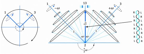
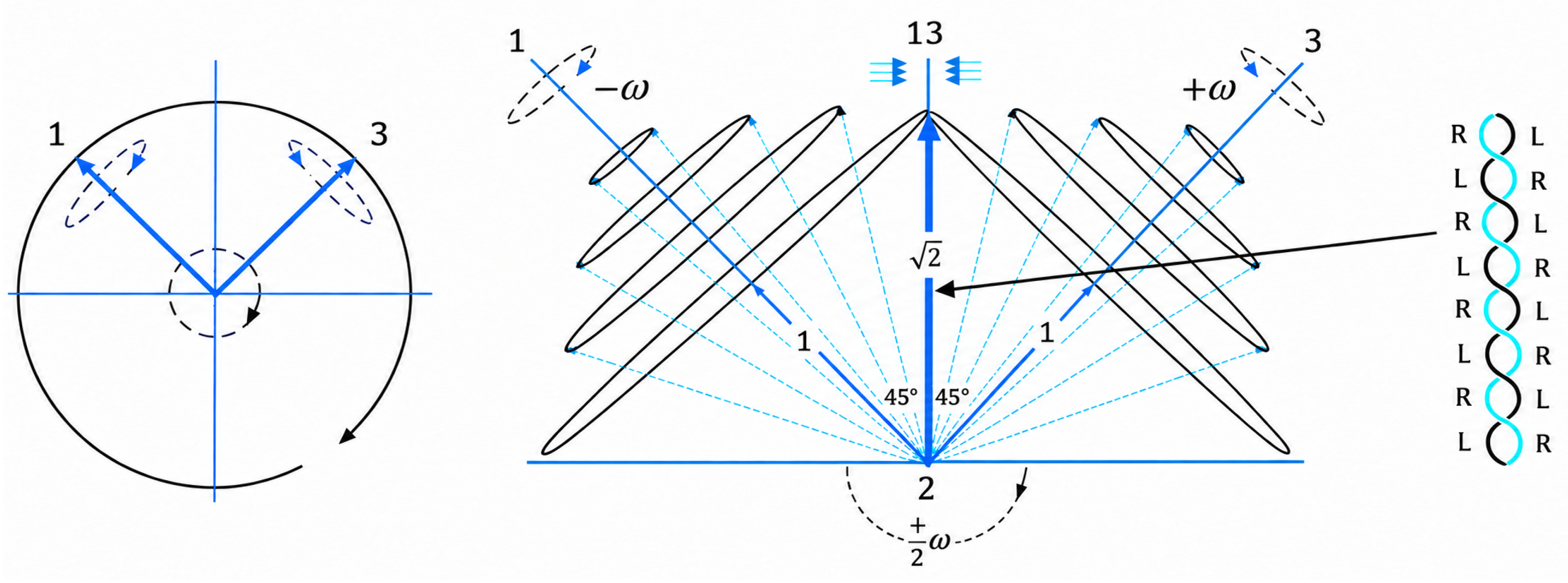
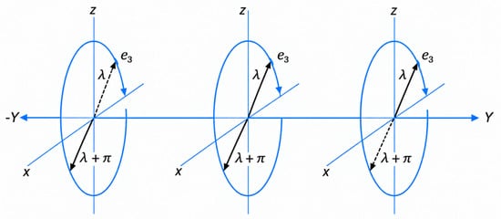
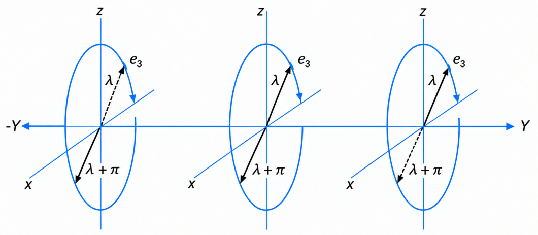
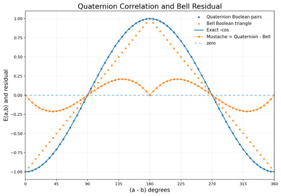
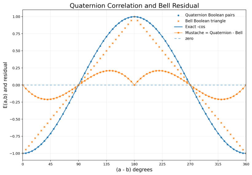
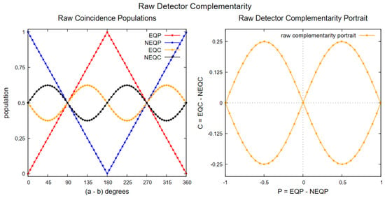
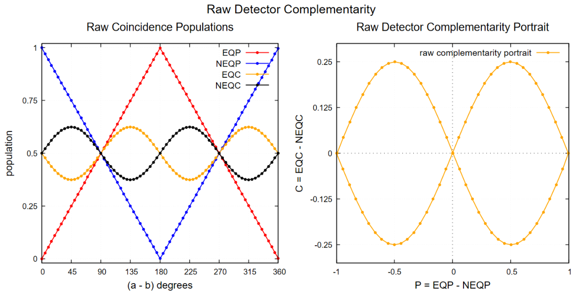
Disclaimer/Publisher’s Note: The statements, opinions and data contained in all publications are solely those of the individual author(s) and contributor(s) and not of MDPI and/or the editor(s). MDPI and/or the editor(s) disclaim responsibility for any injury to people or property resulting from any ideas, methods, instructions or products referred to in the content. |
© 2026 by the author. Licensee MDPI, Basel, Switzerland. This article is an open access article distributed under the terms and conditions of the Creative Commons Attribution (CC BY) license.