A Century of the Schrödinger Equation (1926–2026): Recovering the Wave Picture and Its Physical Intuition

Abstract

One century after Schrödinger’s 1926 papers, the optical–mechanical analogy remains a useful guide to wave mechanics. This pedagogical perspective connects action and phase, stationary states, superposition, field modes, and electromagnetic gauge coupling. Its contribution is a unified account that explicitly separates exact identities, controlled approximations, and heuristic analogies. We distinguish Fourier representations from independently evolving momentum modes, exhibit the assumptions required to recover Hamilton–Jacobi dynamics, and separate classical mode selection from canonical field quantization. Electromagnetic phase factors are presented with their domains of validity, while operational measurement rules are distinguished from interpretative claims. The article proposes neither new dynamics nor a resolution of the measurement problem; it offers a physically motivated route through established results while identifying where classical wave intuition ceases to be sufficient.

1. Introduction

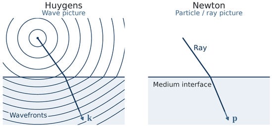
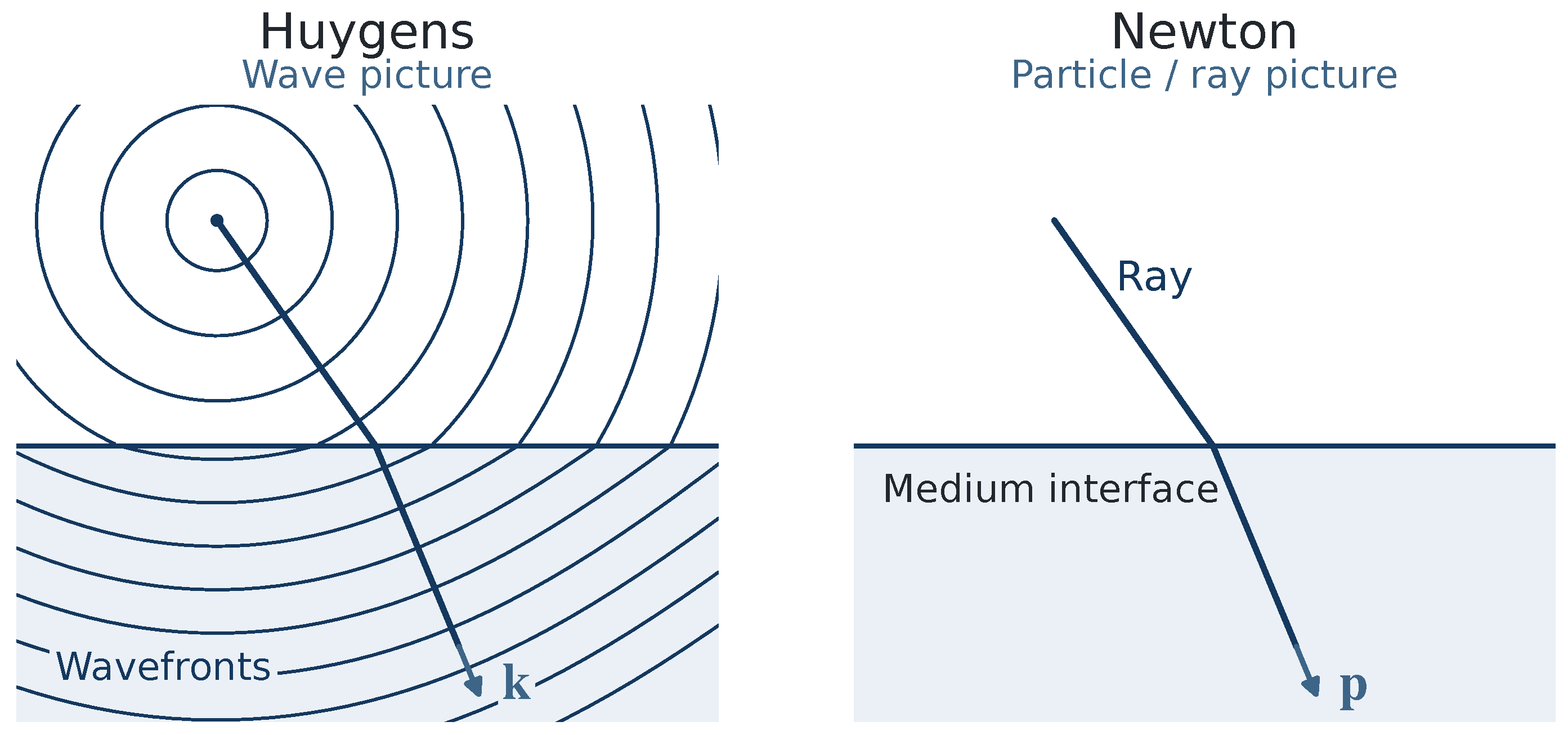
The historical contrast between corpuscular and wave descriptions of light is associated with Newton [1] and Huygens [2]. A different and more precise bridge was established by Hamilton: geometrical optics and classical mechanics possess closely analogous mathematical structures [3,4]. This optical–mechanical analogy predates, and should not be identified with, the later quantum notion of wave–particle complementarity. Its simplest geometrical image is that, in an isotropic medium, an optical ray is orthogonal to the wavefront (Figure 1).

Figure 1. Wave–particle analogy. Light rays can be easily visualized as particle trajectories orthogonal to the light wavefront.

The intended contribution is pedagogical: a connected route from action and phase to stationary modes, quantum excitations, and gauge coupling, with the status of each step made explicit. The target reader is familiar with undergraduate mechanics and wave physics. We distinguish exact reformulations from controlled short-wavelength approximations and from heuristic motivations; no new physical result or interpretation is proposed. This is a selective modern reconstruction, not a claim that the historical discovery followed a unique deductive sequence. Mehra’s specialized study of the creation of wave mechanics places the 1926 work in its historical setting [5]; Beller and Howard document why the later label “Copenhagen interpretation” should not erase disagreements among its associated authors [6,7].

The Schrödinger equation, like Newton’s Second Law, is a fundamental postulate of the theory. It cannot be derived from more basic principles in a strict sense and must be introduced to describe the wave-like nature of matter revealed by quantum phenomena. Many modern textbook “derivations” are primarily pedagogical constructions that reconstruct the equation from later formal structures, rather than reflecting the original conceptual breakthrough. This can partially obscure the historical development of quantum mechanics and the role of physical insight and analogy in its formulation, sometimes giving the misleading impression that major theoretical revolutions emerge as straightforward consequences of established principles.

The Schrödinger equation is typically introduced in textbooks as the fundamental dynamical equation of non-relativistic quantum mechanics (for standard non-relativistic quantum mechanics, see [8,9,10,11,12]). It is motivated by the wave–particle duality and the idea that particles are associated with wave-like behavior. Starting from the classical energy relation for a particle,

$$E={\displaystyle \frac{{\mathbf{p}}^2}{2m}}+V\left(\mathbf{r}\right),$$

(1)

one promotes energy and momentum to operators acting on a wavefunction $\psi (\mathbf{r},t)$.

The promotion of energy and momentum to quantum operators is justified in textbooks by the wave nature of matter and the structure of plane wave solutions. For a free particle, the wavefunction can be written as

$$\psi (\mathbf{r},t)=e^{i(\mathbf{k}·\mathbf{r}-\omega t)}.$$

(2)

Taking derivatives gives

$$i\hslash {\displaystyle \frac{\partial \psi }{\partial t}}=\hslash \omega \psi ,-i\hslash \nabla \psi =\hslash \mathbf{k}\psi .$$

(3)

Using Planck’s and de Broglie’s relations, $E=\hslash \omega$ and $\mathbf{p}=\hslash \mathbf{k}$ respectively, one identifies the canonical substitutions:

$$E\to i\hslash {\displaystyle \frac{\partial }{\partial t}},\mathbf{p}\to -i\hslash \nabla .$$

(4)

It is worth noticing here that one replaces dynamic quantities E and $\mathbf{p}$ with operators acting on functions. This replacement represents a genuine paradigm shift because physical observables are no longer treated as ordinary numbers describing a system. Instead, quantities such as energy and momentum become linear operators acting on the wavefunction. As a result, the state of a system is described by a vector in a Hilbert space rather than by a point in phase space. Physical predictions are obtained from the eigenvalues and expectation values of these operators. Moreover, operators generally do not commute, leading to fundamental uncertainty relations with no classical counterpart.

Applying these operators to the classical Hamiltonian yields the time-dependent Schrödinger equation,

$$i\hslash {\displaystyle \frac{\partial \psi (\mathbf{r},t)}{\partial t}}=\left(-{\displaystyle \frac{{\hslash }^2}{2m}}{\nabla }^2+V(\mathbf{r},\mathbf{t})\right)\psi (\mathbf{r},t).$$

(5)

For a self-adjoint Hamiltonian, this equation governs continuous, deterministic, unitary evolution of the quantum state. The Born rule instead gives probabilities for measurement outcomes: for a normalized spinless one-particle state, ${\left|\psi (\mathbf{r},t)\right|}^2$ is the position probability density. These operational statements do not fix the ontology of the wavefunction. In the textbook description of an ideal projective measurement, the conditional state is updated to the eigenspace associated with the recorded outcome. Whether that update represents a physical collapse, an information update, or an effective subsystem description depends on the interpretation. The tension between unitary evolution of a system plus apparatus and the occurrence of definite records is the measurement problem. Entanglement and violations of Bell inequalities provide additional constraints on classical explanations of quantum correlations; they do not by themselves solve that problem.

For a time-independent Hamiltonian, stationary states are obtained by separation of variables $\psi (\mathbf{r},t)=\varphi \left(\mathbf{r}\right)e^{-iEt/\hslash }$. This leads to the time-independent Schrödinger equation,

$$\left(-{\displaystyle \frac{{\hslash }^2}{2m}}{\nabla }^2+V\left(\mathbf{r}\right)\right)\varphi \left(\mathbf{r}\right)=E\varphi \left(\mathbf{r}\right).$$

(6)

This is an eigenvalue problem for the Hamiltonian operator on a specified domain. Normalizable bound states correspond to point-spectrum eigenvalues; scattering states may belong to a continuous spectrum. Self-adjointness ensures real eigenvalues and generates unitary time evolution; it does not, by itself, imply that the spectrum is non-negative. Thus, the Schrödinger equation provides the quantum analogue of Newtonian dynamics, replacing classical trajectories with the evolution of a wavefunction in Hilbert space [13].

The structure of the article is as follows. In Section 2 the particle–ray analogy in optics is reviewed. In Section 3 the particle–wave analogy in classical mechanics is synoptically sketched. In Section 4 the basic idea of Schrödinger synthesis is presented. Finally, in Section 5, Section 6 and Section 7 the visual power of wave formulation of quantum mechanics is used to clarify some of the conceptual aspects of first and second quantization, and gauge interaction theory, which are often obscured by their abstract and formal presentations in modern textbooks. The entire discussion should, however, be interpreted with due caution, given the conceptually distinct nature of quantum physics compared with the physics of macroscopic phenomena.

2. Optics

A wavefront, indeed, is a surface of constant phase, defined by $\varphi (\mathbf{r},t)=const$. The optical ray represents the direction of energy propagation of the wave. In a homogeneous and isotropic medium, the wavevector is given by $\mathbf{u}=\nabla \varphi (\mathbf{r},t)$. Since $\nabla \varphi (\mathbf{r},t)$ is normal to surfaces of constant phase, it is orthogonal to the wavefronts. Therefore, the wavevector $\mathbf{u}$ is perpendicular to the equi-phase surfaces. Rays are defined as curves tangent to the wavevector direction. Hence, rays are everywhere orthogonal to wavefronts. This is equivalent to the property that gradients are orthogonal to level surfaces. The result holds under the geometrical optics approximation. In anisotropic media, ray and wavevector directions may not coincide, and orthogonality must be treated with care. The optical path length in a medium with refractive index n, from a source to a point $\mathbf{r}$, is defined as

$$S\left(\mathbf{r}\right)={\int }_{\gamma }n\left({\mathbf{r}}^{\prime }\right)\mathrm{d}s,$$

(7)

over the trajectory $\gamma$. For monochromatic light with wavelength $\lambda$, the corresponding accumulated phase is given by $kS$, with $k=2\pi /\lambda$. From Equation (7), two approaches are possible:

• Apply the variational principle $\delta S=0$ to obtain the ray $\gamma$. This is Fermat’s principle: the optical path is stationary with respect to nearby paths, but need not be a minimum [14].
• Determine the wavefront from the scalar field $S\left(\mathbf{r}\right)$ through the equation

  $$|\nabla S(\mathbf{r}\left)\right|=n\left(\mathbf{r}\right),$$

  (8)

  known as the eikonal equation, and determine the corresponding ray, i.e., the direction of the wavevector (the gradient of the wavefront), through the differential equation

  $${\displaystyle \frac{\mathrm{d}\mathbf{r}}{\mathrm{d}s}}={\displaystyle \frac{\nabla S\left(\mathbf{r}\right)}{|\nabla S(\mathbf{r}\left)\right|}}.$$

  (9)

To connect rays to wave propagation, we first note that the eikonal equation, with the constraint $n>0$, is mathematically equivalent to its squared version

$${|\nabla S\left(\mathbf{r}\right)|}^2=n^2\left(\mathbf{r}\right).$$

(10)

For monochromatic waves in the scalar, isotropic approximation, the wave equation reduces to the Helmholtz equation:

$${\nabla }^2\psi \left(\mathbf{r}\right)+k^2{n}^2\left(\mathbf{r}\right)\psi \left(\mathbf{r}\right)=0.$$

(11)

With the ansatz $\psi \left(\mathbf{r}\right)=A\left(\mathbf{r}\right)e^{ikS\left(\mathbf{r}\right)}$, in the limit $k\to \infty$ ($\lambda \to 0$), this equation yields the eikonal equation in the form of Equation (10). In other words, in the limit in which the eikonal equation is derived, the wave propagates as if its energy were concentrated along well-defined trajectories, the rays indeed. In this sense, the behavior resembles that of a particle. In the short-wavelength limit $k\to \infty$, the Laplacian is dominated by the highest-order contributions in k. In particular, one finds

$${\nabla }^2\psi \propto e^{ikS}\left[-k^2{(\nabla S)}^2+\mathcal{O}\left(k\right)\right].$$

(12)

Hence, to leading order,

$${\nabla }^2\psi \sim -k^2{(\nabla S)}^2\psi ,k\to \infty .$$

(13)

The dominant contribution arises because each spatial derivative acting on the rapidly oscillating phase $e^{ikS}$ produces a factor $ik\nabla S$, so that the second derivative yields a term proportional to ${\left(ik\right)}^2{(\nabla S)}^2=-k^2{(\nabla S)}^2$.

In summary, starting from the Helmholtz equation and introducing the eikonal ansatz, one obtains the eikonal equation in the zero-wavelength limit. This equation describes phase propagation in terms of rays, which can be interpreted as geometric trajectories analogous to those of a particle. This formulation is also closely related to Fermat’s variational principle.

3. Mechanics

The action of the environment on a particle is represented in Newtonian mechanics by force. At fixed energy, the same trajectory can be characterized by Maupertuis’ stationary-action principle [15], with abbreviated action

$$S={\int }_A^B\mathbf{p}·\mathrm{d}\mathbf{r}.$$

(14)

In the case of a free particle with constant energy, the Maupertuis principle leads to a particularly simple result. In flat Euclidean space, the geodesics are straight lines, so the physical trajectory connecting two points is simply the straight-line path. Moreover, since the particle is free and its energy is conserved, its speed remains constant along the trajectory. Therefore, the natural motion of a free particle consists of uniform motion along the geodesics of Euclidean space.

In the time-dependent variational formulation one instead uses $\mathcal{S}=\int Ldt$, with $L=K-V$, where K and V are the kinetic and potential energies, respectively; stationary variations give the Euler–Lagrange equations [16]. The abbreviated and Lagrangian actions are related, but should not be identified term by term.

The Lagrangian formulation, in a deeper and more fundamental description, connects to the Hamiltonian formalism and the corresponding Hamilton equations (Hamilton, 1834) [4]. From this formulation, an alternative description of the dynamics of a mechanical system can be given in terms of a generating function of the action, without the need to directly follow the trajectories point by point, through the Hamilton–Jacobi equation

$$H\left(\mathbf{q},{\displaystyle \frac{\partial S(\mathbf{q},t)}{\partial \mathbf{q}}},t\right)+{\displaystyle \frac{\partial S(\mathbf{q},t)}{\partial t}}=0.$$

(15)

If the Hamiltonian does not depend explicitly on time and has the standard classical form

$$H(\mathbf{q},\mathbf{p})={\displaystyle \frac{{\mathbf{p}}^2}{2m}}+V\left(\mathbf{q}\right),$$

(16)

and $S(\mathbf{q},t)=W\left(\mathbf{q}\right)-Et$, with $\mathbf{p}=\nabla W$, Equation (15) reduces to a form mathematically analogous to the eikonal equation:

$${\left|\nabla W\left(\mathbf{q}\right)\right|}^2=2m(E-V\left(\mathbf{q}\right)).$$

(17)

From this point, the interpretation arises by analogy: the particle trajectories can be seen as curves orthogonal to the iso-phase surfaces (wavefronts) defined by the action. In conclusion, the eikonal equation in geometric optics is directly analogous to the Hamilton–Jacobi equation in classical mechanics: both describe the evolution of a phase-like function whose gradients determine the system’s trajectories, emerging as the high-frequency or semiclassical limit of an underlying wave description.

The wave nature of light was consolidated after the discovery of typical wave phenomena such as diffraction and interference. By analogy, one might then wonder whether particles themselves could exhibit similar behavior under certain conditions. These behaviors, known as quantum phenomena, were taken seriously only about 70 years after Hamilton (Planck, 1900) [17]. The physicist who developed this analogy in depth was Erwin Schrödinger in 1926 [18,19,20,21,22].

4. Schrödinger’s Synthesis

In 1926, quantum phenomenology was already remarkably rich. The year before, the first mathematical formulation of quantum mechanics, known as matrix mechanics, had been developed by Heisenberg [23]. Instead of relying on particle orbits and ad hoc quantization rules, as in Bohr’s atomic model [24], Heisenberg introduced a radical paradigm shift. He started from the observable frequencies of atomic transitions, encoded in the Rydberg formula, and constructed the quantum counterpart of classical dynamical variables. In modern notation, position is represented by matrix elements with transition-frequency time dependence, subject to the Ritz combination principle, ${\omega }_{mn}={\omega }_{mk}+{\omega }_{kn}$:

$$x_{mn}\left(t\right)=x_{mn}\left(0\right)e^{i{\omega }_{mn}t},{\omega }_{mn}=(E_m-E_n)/\hslash .$$

(18)

The coefficients $x_{mn}$ naturally combine according to the rules of matrix multiplication (e.g., ${x·y|}_{nm}={\sum }_k{x}_{nk}{y}_{km}$), leading for the first time to a formalism in which physical observables possess discrete spectra and, in general, do not commute. This marked the abandonment of the classical description of dynamical variables in favor of a fundamentally new mathematical framework capable of reproducing the observed quantum phenomena.

At the same time, however, the introduction of matter waves provided an intuitive visual justification for the discretization (quantization) observed in atomic physics, such as the emission of light from discrete energy levels (de Broglie, 1924) [25]. A confined wave, in fact, much like a stretched guitar string, naturally exhibits discrete stationary modes of oscillation. Within this picture, the quantization of angular momentum introduced to explain discrete atomic spectra, $L=n\hslash$, or, more generally, the quantization of the action,

$$\oint \mathbf{p}·\mathrm{d}\mathbf{q}=nh=2\pi n\hslash ,$$

(19)

seemed to find a simple wave interpretation. This historical condition is only approximate; more refined semiclassical rules include phase corrections at turning points.

Once the wave is chosen as a possible paradigm, the task for a physicist aiming to complete the theory becomes much clearer. Just as Maxwell’s equations, through the Helmholtz equation, lead to the eikonal equation, one must, by a reverse-engineering approach, understand how to obtain the analogue of a wave equation for a particle. The attentive reader, familiar with the Schrödinger equation, will likely have experienced a moment of surprise upon seeing (13). It is precisely from there that one must start. The following modern reconstruction isolates the optical–mechanical motivation; the actual sequence of Schrödinger’s 1926 arguments was more involved [5].

In analogy with light waves, one is led to associate the mechanical action with the phase of a wave,

$$\psi (\mathbf{r},t)=A(\mathbf{r},t)e^{iS(\mathbf{r},t)/\hslash }.$$

(20)

Initially take A and S real and sufficiently differentiable on a region where $A>0$. The phase S need not initially satisfy a classical equation. For stationary motion, write $S=W-Et$ and take A time-independent. Applying the product rule twice gives the exact identity

$${\displaystyle \frac{{\nabla }^2\left(A{e}^{iW/\hslash }\right)}{A{e}^{iW/\hslash }}}={\displaystyle \frac{{\nabla }^{2}A}{A}}-{\displaystyle \frac{{|\nabla W|}^2}{{\hslash }^2}}+{\displaystyle \frac{i}{\hslash }}\left(2{\displaystyle \frac{\nabla A}{A}}·\nabla W+{\nabla }^{2}W\right).$$

(21)

In a classically allowed region let $p=|\nabla W|>0$. If the amplitude and momentum vary on a length scale L with $pL\gg \hslash$, the amplitude-curvature term is small relative to $p^2/{\hslash }^2$, while the phase-transport terms are of lower asymptotic order. The leading term is then ${\nabla }^2\psi \simeq -p^2\psi /{\hslash }^2$. Substituting the classical relation $p^2=2m(E-V)$ gives ${\nabla }^2\psi \simeq -2m(E-V)\psi /{\hslash }^2$. Multiplying by $-{\hslash }^2/\left(2m\right)$ and moving $V\psi$ to the left motivates

$$-{\displaystyle \frac{{\hslash }^2}{2m}}{\nabla }^2\psi +V\psi =E\psi .$$

(22)

Adopting this as an exact wave equation is an additional physical postulate, not a consequence of the approximate preceding equality. The amplitude at the next order must also satisfy a transport equation; it cannot be chosen arbitrarily.

The phase normalization is fixed empirically by the Planck and de Broglie relations. For a free particle with action

$$S(\mathbf{r},t)=\mathbf{p}·\mathbf{r}-Et.$$

(23)

For this case $S/\hslash =\mathbf{k}·\mathbf{r}-\omega t$ when $\mathbf{p}=\hslash \mathbf{k}$ and $E=\hslash \omega$, precisely the de Broglie and Planck relations.

For the time-dependent ansatz, the product rule also gives the exact identity

$${\displaystyle \frac{i\hslash {\partial }_t\psi }{\psi }}=i\hslash {\displaystyle \frac{{\partial }_{t}A}{A}}-{\partial }_{t}S.$$

(24)

At leading semiclassical order the right-hand side is $-{\partial }_{t}S$, while the leading action of $-{\hslash }^2{\nabla }^2/\left(2m\right)+V$ on $\psi$, divided by $\psi$, is ${|\nabla S|}^2/\left(2m\right)+V$. Hamilton–Jacobi theory equates these two leading expressions. Matching them motivates the time-dependent wave equation; it does not determine the exact quantum dynamics or its amplitude terms from classical mechanics alone.

Including time dependence suggests the full Schrödinger equation, adopted here as the quantum dynamical postulate rather than derived from Hamilton–Jacobi theory

$$\left(-{\displaystyle \frac{{\hslash }^2}{2m}}{\nabla }^2+V(\mathbf{r},t)\right)\psi (\mathbf{r},t)=i\hslash {\displaystyle \frac{\partial \psi (\mathbf{r},t)}{\partial t}}.$$

(25)

The reverse connection can be stated exactly. Substitution of Equation (20) into the Schrödinger equation, for real V, yields

$${\partial }_{t}S+{\displaystyle \frac{{|\nabla S|}^2}{2m}}+V+Q=0,Q=-{\displaystyle \frac{{\hslash }^2}{2m}}{\displaystyle \frac{{\nabla }^{2}A}{A}},$$

(26)

and the exact continuity equation

$${\partial }_t\left(A^2\right)+\nabla ·\left(A^2{\displaystyle \frac{\nabla S}{m}}\right)=0.$$

(27)

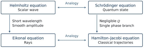
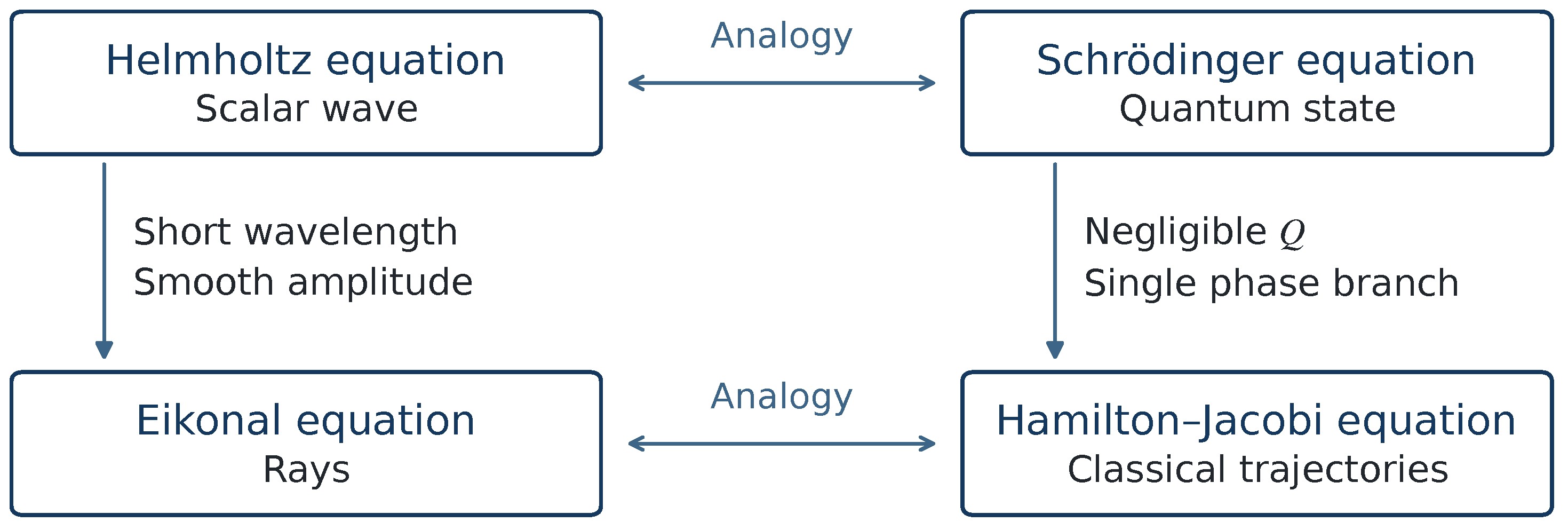
The Hamilton–Jacobi equation follows approximately when Q is negligible compared with the relevant local kinetic or action-variation scale. A useful local criterion is ${\hslash }^2\left|{\nabla }^{2}A\right|/A\ll p^2$, with $p=|\nabla S|$, together with smooth phase gradients and a consistent amplitude transport. In one-dimensional WKB notation, $\hslash |p^{\prime }|/p^2\ll 1$ is a familiar slow-variation condition. These are local conditions, not a conclusion obtained simply by writing $\hslash \to 0$ for an arbitrary family of states. They can fail at nodes ($A=0$), turning points ($p=0$), caustics, and interference between distinct phase branches. The polar equations are exact only away from nodes; a trajectory description additionally requires a suitable single-phase semiclassical state. This conditional reduction is the mechanical analogue of geometrical optics (Figure 2).

Figure 2. Optical–mechanical analogy. Helmholtz theory reduces to the eikonal description in the short-wavelength limit, while Schrödinger dynamics reduces to Hamilton–Jacobi theory when the quantum-potential term is negligible. Horizontal arrows indicate analogies. Both vertical reductions require smoothness and the local conditions discussed in the text; an absolute inequality $S\gg \hslash$ alone is insufficient.

The conventional name “quantum of action” does not mean that every action is an integer multiple of ℏ. A free particle on ${\mathbb{R}}^3$ has continuous momentum and energy spectra, while ℏ still sets the phase scale and enters the canonical commutator. Discreteness must be established for a specified observable and operator domain.

Operationally, for a normalized one-particle state, the probability of finding the particle in a region $\mathsf{\Omega }$ is ${\int }_{\mathsf{\Omega }}{\left|\psi (\mathbf{r},t)\right|}^2{d}^{3}r$. Relative phase affects interference. The wavefunction is a position representation of a state vector; for several particles it is defined on configuration space, usually with additional spin indices, rather than being a scalar wave in ordinary three-dimensional space.

The historical and interpretive claims require separate care. Schrödinger’s early continuous-wave proposals and Born’s 1926 probabilistic treatment of scattering were distinct contributions [5,18,26]. They should not be compressed into a single conversion to a unified “Copenhagen” doctrine in 1926. The latter label groups differing positions, including Bohr’s complementarity [27] and Heisenberg’s formulations [6,7]. Everettian approaches retain universal unitary evolution; Bohmian approaches supplement a guiding wavefunction with a particle configuration; collapse models modify the dynamics. These positions assign different roles to the state and do not all make identical dynamical claims. The Wigner function, by contrast, is a phase-space representation of quantum states, not by itself a competing interpretation. It can take negative values, but not every quantum state has a negative Wigner function.

To state the measurement problem explicitly, ideal unitary coupling maps an initial superposition and a ready apparatus state to ${\sum }_i{c}_i|i⟩|M_i⟩$. The operational rule assigns probability $|c_i{|}^2$ to record i for normalized coefficients and orthonormal alternatives. Decoherence suppresses interference between apparatus records in a reduced description, but does not by itself select one term of the global state. A physical collapse is one possible additional account; it is not an interpretation-independent consequence of the Schrödinger equation. Our wave analogies clarify the linear dynamics but do not resolve the emergence or interpretation of definite records.

5. Visual Power of the Wave Formulation

The validity of the Schrödinger equation extends beyond the plane-wave solution describing a free particle. Independently of the dynamics, a square-integrable wavefunction on ${\mathbb{R}}^3$ admits a Fourier representation in the $L^2$ sense (pointwise under stronger regularity assumptions),

$$\psi (\mathbf{r},t)={\displaystyle \frac{1}{{\left(2\pi \right)}^{3/2}}}{\int }_{{\mathbb{R}}^3}\tilde{\psi }(\mathbf{k},t)e^{i\mathbf{k}·\mathbf{r}}{d}^{3}k,$$

(28)

where $\tilde{\psi }$ denotes the Fourier transform with the displayed symmetric normalization. Linearity permits superposition of solutions, but does not make an arbitrary basis diagonal in the Hamiltonian. For a spatially dependent potential one instead obtains

$$i\hslash {\partial }_t\tilde{\psi }(\mathbf{k},t)={\displaystyle \frac{{\hslash }^2{\left|\mathbf{k}\right|}^2}{2m}}\tilde{\psi }(\mathbf{k},t)+{\displaystyle \frac{1}{{\left(2\pi \right)}^{3/2}}}\int d^3{k}^{\prime }\tilde{V}(\mathbf{k}-{\mathbf{k}}^{\prime },t)\tilde{\psi }({\mathbf{k}}^{\prime },t).$$

(29)

Here $\tilde{V}$ uses the same Fourier convention; distributional interpretation may be required for non-integrable potentials. The convolution generally couples momenta. Independent evolution holds when the Hamiltonian is diagonal in momentum, as for a free particle or a spatially uniform potential. In the free case,

$$\tilde{\psi }(\mathbf{k},t)=\tilde{\psi }(\mathbf{k},0)e^{-iE\left(\mathbf{k}\right)t/\hslash },E\left(\mathbf{k}\right)={\displaystyle \frac{{\hslash }^2{\left|\mathbf{k}\right|}^2}{2m}}.$$

(30)

For a general time-independent self-adjoint Hamiltonian, its own spectral representation provides the corresponding energy phases, with both discrete and continuous parts where appropriate.

The complex structure of standard quantum mechanics organizes phase relations and unitary evolution. A single real scalar wavefunction with the same Schrödinger evolution is generally not sufficient: the time derivative mixes two real components. Unitarity follows from self-adjointness of the Hamiltonian together with the Schrödinger evolution law; the conserved quantity is the total probability ${\int \left|\psi \right|}^2{d}^{3}r$, while the local density can change by probability flow. Rewriting a complex state as two real functions remains possible if its complex structure and observables are retained. This is different from replacing the theory by one on a genuinely real Hilbert space with different composition rules [28]. Such distinctions also matter in broader discussions of quantum theory in “theoryspace” [29].

One may wonder whether the complex structure takes us completely beyond any possible physical visualization. However, an interesting analogy is provided by Maxwell’s equations, which can also be written in a compact complex form. Introducing the Riemann–Silberstein vector

$$\mathbf{F}=\mathbf{E}+ic\mathbf{B},$$

(31)

where $\mathbf{E}$ and $\mathbf{B}$ are the electric and magnetic fields, respectively, the vacuum Maxwell equations become

$$\begin{array}{cc}\hfill i{\displaystyle \frac{\partial \mathbf{F}}{\partial t}}& =c\nabla \times \mathbf{F},\hfill \end{array}$$

(32)

$$\begin{array}{cc}\hfill \nabla ·\mathbf{F}& =0.\hfill \end{array}$$

(33)

This formulation closely resembles the Schrödinger equation and highlights the role played by the imaginary unit in generating rotations between the electric and magnetic fields. Unlike quantum mechanics, however, the complex field $\mathbf{F}$ is merely a convenient mathematical representation: the fundamental physical quantities remain the two independent, real, and “observable” vector fields $\mathbf{E}$ and $\mathbf{B}$. For a Hamiltonian with real coefficients, such as $\widehat{H}=-{\hslash }^2{\nabla }^2/\left(2m\right)+V$ with real V and no vector potential, if one writes $\psi (\mathbf{r},t)=u(\mathbf{r},t)+iv(\mathbf{r},t)$, the Schrödinger equation can be recast as the following system of real equations:

$$\begin{array}{cc}\hfill \hslash {\displaystyle \frac{\partial u(\mathbf{r},t)}{\partial t}}& =\widehat{H}v(\mathbf{r},t),\hfill \end{array}$$

(34)

$$\begin{array}{cc}\hfill \hslash {\displaystyle \frac{\partial v(\mathbf{r},t)}{\partial t}}& =-\widehat{H}u(\mathbf{r},t).\hfill \end{array}$$

(35)

Indeed, $i\hslash ({\partial }_{t}u+i{\partial }_{t}v)=\widehat{H}u+i\widehat{H}v$ implies $-\hslash {\partial }_{t}v=\widehat{H}u$ and $\hslash {\partial }_{t}u=\widehat{H}v$. For an energy eigenfunction f with real profile, $\psi =f{e}^{-iEt/\hslash }$ gives $u=f\cos (Et/\hslash )$ and $v=-f\sin (Et/\hslash )$, consistently with both signs. For complex-coefficient Hamiltonians one must first split the operator itself into real and imaginary parts. This is analogous to Maxwell’s equations written in terms of $\mathbf{E}$ and $\mathbf{B}$, with the important difference that u and v are not separately observable. The two equations have the form of Hamilton equations for a pair of variables with a symplectic structure. This provides another useful, although formal, visualization of the internal phase degree of freedom.

Once the wave formulation is assumed, several relations become visually accessible. For position and momentum, the uncertainty relation follows from their Fourier relation and the Cauchy–Schwarz inequality. More general uncertainty relations are operator statements and need not involve Fourier-conjugate variables.

Boundary conditions help specify an operator domain, but do not alone guarantee a discrete spectrum: a free particle on a half-line with a reflecting endpoint still has a continuous energy spectrum. Finite spatial boundaries are not necessary either: the harmonic oscillator on the whole real line has a discrete spectrum because of its confining potential and square-integrability requirement. Spin provides a further example of discrete outcomes not derived from spatial standing waves. Thus boundary conditions are neither a necessary nor a sufficient general explanation of quantum discreteness. Atomic orbitals are normalizable stationary waves in the Coulomb potential. Landau levels, arising from the transverse motion of a charged particle in a uniform magnetic field, have the mathematical structure of a harmonic oscillator and can therefore also be visualized through wave modes.

Orbital angular momentum quantization can be related to the matching of the wavefunction under a full rotation. Spin requires a more abstract wave space. Quantum states transform under representations of $SU\left(2\right)$, the double cover of $SO\left(3\right)$, and half-integer-spin state vectors acquire a minus sign under a $2\pi$ rotation, returning to the same vector after $4\pi$. Since physical pure states are rays, that global sign is not observable by itself, although relative phases can be detected interferometrically. One may therefore retain a wave intuition only in an extended sense: the spinor has a phase structure in an internal space, not the shape of an ordinary standing wave in three-dimensional space. The analogy is useful precisely when this limitation is kept explicit.

Finally, quantum superposition has no complete classical analogue. Indeed, it is, in a certain sense, a neologism describing a genuinely quantum-mechanical phenomenon. However, if one considers waves, the concept is closely related to the classical principle of superposition, which follows directly from the linear structure of the wave equation in both classical and quantum physics. A classical example of superposition can be illustrated by considering a string fixed at both ends. The normal modes of the string form a complete set of solutions to the wave equation, and because the system is linear, any linear combination of these modes is itself a valid solution. For example, if the first normal mode is excited with a relative amplitude of $70\%$ and the second with $30\%$, the motion of the string is described by

$$y(x,t)=0.7y_1(x,t)+0.3y_2(x,t).$$

(36)

From a mathematical perspective, this is analogous to a quantum state written as a linear combination of two eigenstates,

$$|\psi ⟩=\alpha |1⟩+\beta |2⟩.$$

(37)

In both cases, the state of the system is represented as a superposition of basis states, reflecting the underlying linearity of the governing equations. However, the analogy has an important limitation. For the vibrating string, both normal modes are physically present and can, in principle, be observed simultaneously. A measurement of the string’s position simply reveals the combined oscillation without altering the state of the system. In quantum mechanics, by contrast, a measurement associated with the eigenstates $|1⟩$ and $|2⟩$ yields only one of the possible outcomes, with probabilities ${\left|\alpha \right|}^2$ and ${\left|\beta \right|}^2$, respectively. For a normalized state in an orthonormal basis, an ideal projective measurement is described operationally by conditioning the state on the corresponding eigenstate; a physical collapse is an interpretation-dependent account of that update. A similar behavior could only be reproduced for the vibrating string by introducing an external device that randomly selects one normal mode while suppressing the other. The distinction concerns quantum measurement statistics and state conditioning; interpreting definite records remains part of the measurement problem discussed in Section 4. More fundamentally, it remains an open question whether the wavefunction $\psi$ represents an ontic physical entity or merely an epistemic description of our knowledge of the system. Nevertheless, even under the most conservative epistemic interpretation, the physical phenomena associated with quantum superposition can still be meaningfully visualized through classical analogies, provided that their limitations are kept in mind.

6. From Classical Wave Modes to Second Quantization

The central point of the wave picture becomes especially clear for harmonic motion. Before introducing quantum operators, consider a purely classical wave whose propagation is confined by a quadratic restoring term. A simple illustrative equation is

$${\displaystyle \frac{{\partial }^{2}u}{\partial t^2}}-v^2{\displaystyle \frac{{\partial }^{2}u}{\partial x^2}}+{\mathsf{\Omega }}_0^2{\displaystyle \frac{x^2}{{\ell }^2}}u=0,$$

(38)

where v is a wave velocity, ${\mathsf{\Omega }}_0$ is a frequency scale, and ℓ is a length scale. This equation is not proposed as a microscopic model of a specific material: it is a dimensionally consistent toy model designed to isolate the mode structure. With $u(x,t)=X\left(x\right)e^{-i\omega t}$ one obtains

$$-v^2{X}^{″}+{\mathsf{\Omega }}_0^2{\displaystyle \frac{x^2}{{\ell }^2}}X={\omega }^{2}X.$$

(39)

The spatial profiles are Hermite–Gaussian functions and the admissible normal-mode frequencies satisfy

$${\omega }_n^2=(2n+1){\displaystyle \frac{v{\mathsf{\Omega }}_0}{\ell }},n=0,1,2,\dots .$$

(40)

Thus a classical wave problem can already possess a discrete set of normal modes. This is sometimes called “classical quantization”, but the phrase must be used cautiously: the classical energy stored in each mode remains continuous because its amplitude is arbitrary. What is discrete here is the set of allowed mode shapes and frequencies, not the amount of energy carried by a mode.

Now consider the one-dimensional stationary Schrödinger equation of the harmonic oscillator,

$$-{\displaystyle \frac{{\hslash }^2}{2m}}{\displaystyle \frac{d^2\psi \left(x\right)}{d{x}^2}}+{\displaystyle \frac{1}{2}}m{\omega }^2{x}^2\psi \left(x\right)=E\psi \left(x\right),$$

(41)

Mathematically, this is the same type of differential eigenvalue problem. Square integrability selects Hermite–Gaussian wavefunctions, but now the eigenvalue is the physical energy,

$$E_n=\hslash \omega \left(n+{\displaystyle \frac{1}{2}}\right),n=0,1,2,\dots$$

(42)

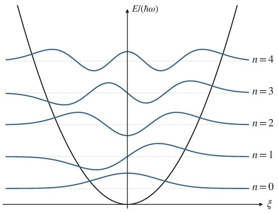
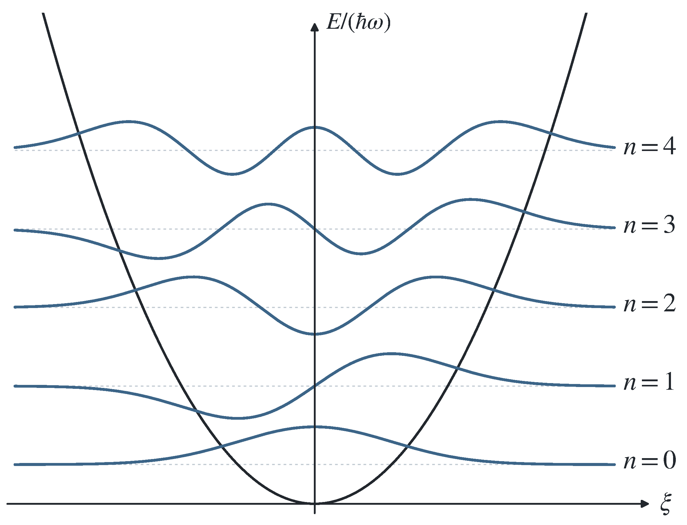
Figure 3 illustrates the result. The visual analogy is powerful: in both the classical and quantum problems, confinement and regularity select a discrete hierarchy of wave profiles. Its limitation is equally important: only in the quantum problem does the eigenvalue represent an energy that comes in units of $\hslash \omega$.

Figure 3. Harmonic-oscillator eigenfunctions, displaced vertically to align them with their equally spaced energy levels. The dimensionless coordinate is $\xi =\sqrt{m\omega /\hslash }x$; the profiles share an arbitrary common vertical scale. The picture emphasizes the mode structure behind the spectrum.

This is the physical picture that the operator language subsequently compresses. Define dimensionless operators

$$\widehat{X}=\sqrt{{\displaystyle \frac{m\omega }{\hslash }}}\widehat{x},\widehat{P}={\displaystyle \frac{\widehat{p}}{\sqrt{m\hslash \omega }}},[\widehat{X},\widehat{P}]=i,$$

(43)

and

$$\widehat{a}={\displaystyle \frac{\widehat{X}+i\widehat{P}}{\sqrt{2}}},{\widehat{a}}^{†}={\displaystyle \frac{\widehat{X}-i\widehat{P}}{\sqrt{2}}}.$$

(44)

Then $[\widehat{a},{\widehat{a}}^{†}]=1$ and

$$\widehat{H}=\hslash \omega \left({\widehat{a}}^{†}\widehat{a}+{\displaystyle \frac{1}{2}}\right).$$

(45)

For the one-particle oscillator, these operators connect different energy eigenfunctions of the same Hamiltonian; they do not create additional particles. Their algebra uses the quantum postulate $[\widehat{x},\widehat{p}]=i\hslash$, not merely the existence of classical normal modes. The algebra is a compact expression of the already quantized oscillator [30,31,32].

For a free field the oscillator construction applies to each independent physical normal coordinate. To make the electromagnetic constraints explicit, consider source-free vacuum radiation in a periodic volume $\mathcal{V}$, with the zero-momentum static sector excluded. In Coulomb gauge, $\nabla ·\mathbf{A}=0$, Gauss’s law removes an independent longitudinal radiative degree of freedom; we choose $\varphi =0$ for this free radiative sector. Each nonzero $\mathbf{k}$ has two transverse polarizations $\lambda =1,2$. A real standing-wave basis supplies independent canonical pairs $(Q_j,P_j)$, with a normalization chosen so that

$$H_{\mathrm{cl}}={\displaystyle \frac{1}{2}}\sum _j(P_j^2+{\omega }_j^2{Q}_j^2),\{Q_j,P_l\}={\delta }_{jl}.$$

(46)

Here j labels independent real modes. Classical $Q_j$ and $P_j$ remain continuous. The additional canonical quantization postulate is

$$[{\widehat{Q}}_j,{\widehat{P}}_l]=i\hslash {\delta }_{jl},[{\widehat{Q}}_j,{\widehat{Q}}_l]=[{\widehat{P}}_j,{\widehat{P}}_l]=0.$$

(47)

Consequently ${\widehat{a}}_j=\sqrt{{\omega }_j/(2\hslash )}{\widehat{Q}}_j+i{\widehat{P}}_j/\sqrt{2\hslash {\omega }_j}$ obeys $[{\widehat{a}}_j,{\widehat{a}}_l^{†}]={\delta }_{jl}$. A unitary change from standing to travelling modes gives the normalized field expansion in SI units [33]:

$$\widehat{\mathbf{A}}(\mathbf{r},t)=\sum _{\mathbf{k},\lambda }\sqrt{{\displaystyle \frac{\hslash }{2{ϵ}_0\mathcal{V}{\omega }_k}}}\left[{ϵ}_{\mathbf{k}\lambda }{\widehat{a}}_{\mathbf{k}\lambda }{e}^{i(\mathbf{k}·\mathbf{r}-{\omega }_{k}t)}+{ϵ}_{\mathbf{k}\lambda }^{\ast }{\widehat{a}}_{\mathbf{k}\lambda }^{†}{e}^{-i(\mathbf{k}·\mathbf{r}-{\omega }_{k}t)}\right],$$

(48)

where ${\omega }_k=c\left|\mathbf{k}\right|$, $\mathbf{k}·{ϵ}_{\mathbf{k}\lambda }=0$, and ${ϵ}_{\mathbf{k}\lambda }^{\ast }·{ϵ}_{\mathbf{k}{\lambda }^{\prime }}={\delta }_{\lambda {\lambda }^{\prime }}$. Thus

$$\widehat{H}=\sum _{\mathbf{k},\lambda }\hslash {\omega }_k\left({\widehat{a}}_{\mathbf{k}\lambda }^{†}{\widehat{a}}_{\mathbf{k}\lambda }+{\displaystyle \frac{1}{2}}\right).$$

(49)

The infinite vacuum-energy sum requires regularization when its absolute value is at issue. A finite mode cutoff suffices for the oscillator argument here. The periodic box discretizes mode labels for convenience; photons also exist in the infinite-volume limit, where wavevectors are continuous. Occupation numbers, rather than wavevectors or classical amplitudes, are integer-valued after quantization:

$${\widehat{a}}_j^{†}|n_j⟩=\sqrt{n_j+1}|n_j+1⟩,{\widehat{a}}_j|n_j⟩=\sqrt{n_j}|n_j-1⟩.$$

(50)

These are operator actions in Fock space [34], not a consequence of merely replacing a classical complex coefficient by a hat. For free radiation they add or remove a photon in a specified transverse mode. This bosonic construction does not establish fermionic anticommutation relations; fermionic fields require a different quantization algebra. Interacting gauge theories require their own treatment of constraints and cannot be inferred from this free-field example.

Vibrations in a crystal provide a particularly concrete bridge. A classical lattice supports collective normal modes; after quantization, the occupation of each mode changes in integer steps and the quanta are called phonons. The atoms of the crystal do not individually become phonons: the phonon is the quantum of a collective wave mode. In the same approximate but illuminating sense, elementary particles in a free quantum field are quanta of its normal modes. Interactions and curved or time-dependent backgrounds make the notion of a particle more subtle, but they do not erase the usefulness of this picture.

This is the central intuitive content of second quantization: the operator formalism does not replace the wave picture but encodes, with great efficiency, the possible excitation numbers of its modes. The statement is not that every quantum wave is a literal material vibration in ordinary space; rather, wave-like mode structure persists from classical fields to quantum fields, even when the relevant configuration space is abstract.

7. Gauge Interactions

Electromagnetic coupling illustrates the usefulness and limits of phase intuition. A local phase is gauge-dependent. In a general field, coupling changes the full state, including its amplitude and probability current; it cannot be represented by multiplying a free solution by a local phase. For a spinless particle of charge q, minimal coupling gives

$$i\hslash {\partial }_t\psi =\left[{\displaystyle \frac{{(-i\hslash \nabla -q\mathbf{A})}^2}{2m}}+q\varphi \right]\psi .$$

(51)

The following two distinct restricted constructions must therefore be read with their assumptions. First, if $\mathbf{A}=0$ and $\varphi =\varphi \left(t\right)$ is spatially uniform, the scalar term commutes with the remaining free Hamiltonian and the exact solution is

$$\psi (\mathbf{r},t)=\exp \left[-{\displaystyle \frac{iq}{\hslash }}{\int }_{t_0}^t\varphi \left(t^{\prime }\right)d{t}^{\prime }\right]{\psi }_{\mathrm{free}}(\mathbf{r},t).$$

(52)

A general $\varphi (\mathbf{r},t)$ cannot be factored out this way, because spatial differentiation acts on its position-dependent phase. Second, a spatial connection defines a parallel-transport factor along a specified path $\gamma$ at fixed time,

$$U_{\gamma }=\exp \left[{\displaystyle \frac{iq}{\hslash }}{\int }_{\gamma }\mathbf{A}·d\mathbf{r}\right].$$

(53)

This is a transport factor, not a general solution $\psi =U_{\gamma }{\psi }_{\mathrm{free}}$. Such a local multiplicative solution exists for a pure gauge $\mathbf{A}=\nabla \chi$, $\varphi =-{\partial }_t\chi$ on a suitable simply connected region, where $\psi =e^{iq\chi /\hslash }{\psi }_{\mathrm{free}}$. When the field strength is nonzero the potentials cannot generally be removed by this transformation. Even a locally pure gauge can have nontrivial holonomy on a multiply connected accessible region.

For a prescribed spacetime path, the electromagnetic contribution to the action is $S_{\mathrm{int}}=q\int (\mathbf{A}·d\mathbf{r}-\varphi dt)$. Its phase factor is useful in path integrals or in a semiclassical path approximation; full propagation also involves the kinetic action and, in general, a sum over paths and changing amplitudes. For $\psi =A{e}^{iS/\hslash }$, the exact gauge-coupled polar equation away from nodes is

$${\partial }_{t}S+{\displaystyle \frac{{|\nabla S-q\mathbf{A}|}^2}{2m}}+q\varphi +Q=0,\mathbf{j}={\displaystyle \frac{A^2}{m}}(\nabla S-q\mathbf{A}).$$

(54)

Here Q is defined in Equation (26); A without boldface denotes the amplitude, not the vector potential. The continuity equation is ${\partial }_t{A}^2+\nabla ·\mathbf{j}=0$. Neglecting Q under the conditions of Section 4 recovers charged-particle Hamilton–Jacobi dynamics and hence the Lorentz force. Thus phase geometry complements the force description.

In the static magnetic Aharonov–Bohm arrangement, two coherent paths enclose flux confined to an inaccessible region, while the magnetic field vanishes along the paths. Their gauge-invariant relative phase contribution is [35]

$$\Delta \phi ={\displaystyle \frac{q}{\hslash }}\oint \mathbf{A}·d\mathbf{r}={\displaystyle \frac{q{\mathsf{\Phi }}_B}{\hslash }}\left(\mathrm{mod}2\pi \right).$$

(55)

The contour orientation fixes the sign of ${\mathsf{\Phi }}_B$. The observed fringe shift probes the holonomy, not the potential at a single point. Equality of local densities under a gauge change must be distinguished from the physical evolution of densities in an applied field.

Under the simultaneous transformations

$${\mathbf{A}}^{\prime }=\mathbf{A}+\nabla \chi ,{\varphi }^{\prime }=\varphi -{\partial }_t\chi ,{\psi }^{\prime }=e^{iq\chi /\hslash }\psi ,$$

(56)

Equation (51), ${\left|\psi \right|}^2$, and $\mathbf{j}$ transform consistently, with the latter two invariant. An open-path $U_{\gamma }$ transforms by endpoint phases; a closed-loop factor is gauge-invariant for single-valued admissible transformations.

For clarity, a compatible SI spacetime convention is $x^0=ct$, metric $(+---)$, ${\mathcal{A}}_{\mu }=(-\varphi /c,\mathbf{A})$, and ${\partial }_{\mu }=(c^{-1}{\partial }_t,\nabla )$. Then

$$D_{\mu }={\partial }_{\mu }-{\displaystyle \frac{iq}{\hslash }}{\mathcal{A}}_{\mu },{\mathcal{A}}_{\mu }^{\prime }={\mathcal{A}}_{\mu }+{\partial }_{\mu }\chi ,{\left(D_{\mu }\psi \right)}^{\prime }=e^{iq\chi /\hslash }{D}_{\mu }\psi .$$

(57)

In particular $i\hslash D_t=i\hslash {\partial }_t-q\varphi$ and $-i\hslash \mathbf{D}=-i\hslash \nabla -q\mathbf{A}$, where $D_t=c{D}_0$. The curvature and free electromagnetic Lagrangian density are

$${\mathcal{F}}_{\mu \nu }={\partial }_{\mu }{\mathcal{A}}_{\nu }-{\partial }_{\nu }{\mathcal{A}}_{\mu },{\mathcal{L}}_{\mathrm{EM}}=-{\displaystyle \frac{1}{4{\mu }_0}}{\mathcal{F}}_{\mu \nu }{\mathcal{F}}^{\mu \nu }={\displaystyle \frac{{ϵ}_0}{2}}{\left|\mathbf{E}\right|}^2-{\displaystyle \frac{1}{2{\mu }_0}}{\left|\mathbf{B}\right|}^2.$$

(58)

Here ${\mathcal{F}}_{0i}=-E_i/c$ and ${\mathcal{F}}_{ij}={ϵ}_{ijk}{B}_k$. The Lagrangian is not the energy density, which is $u_{\mathrm{EM}}={ϵ}_0{\left|\mathbf{E}\right|}^2/2+{\left|\mathbf{B}\right|}^2/\left(2{\mu }_0\right)$. Local curvature and global holonomy identify the observable content of the connection picture; neither licenses a general phase-only solution of the interacting dynamics.

8. Conclusions

The optical–mechanical analogy offers a coherent pedagogical route through wave mechanics: action suggests a phase, stationary spectral problems organize bound states, and mode coordinates connect classical fields with quantum excitations. Our contribution is to follow that route while stating the logical status and limits of each connection. It is a modern explanatory reconstruction, not a deduction of quantum mechanics from classical mechanics or a complete history of its discovery.

Several distinctions are essential. Hamilton–Jacobi dynamics follows locally from Schrödinger dynamics only under semiclassical conditions on amplitude and phase. A Fourier representation exists independently of whether its components evolve separately. Boundary conditions and confinement can select discrete spectra, but they neither explain all quantum discreteness nor quantize a classical mode’s energy. Field occupation numbers become discrete only after quantum commutation relations are imposed on independent physical degrees of freedom.

Electromagnetic phase intuition is similarly conditional: a removable pure gauge, a transport factor along a path, and dynamical propagation in a nonzero field are different constructions. Gauge-invariant currents, field strengths, and holonomies identify their physical content. For many-particle states and spin, the wave picture must refer to configuration and internal spaces rather than to an ordinary material wave.

These qualifications preserve the useful visual connections without assigning them explanatory powers they do not have. The wave viewpoint illuminates established quantum structure; it does not by itself settle the ontology of the quantum state or explain definite measurement records.

References

- Newton, I. Opticks: Or, a Treatise of the Reflexions, Refractions, Inflexions and Colours of Light; Royal Society: London, UK, 1704. [Google Scholar]
- Huygens, C. Traité de la Lumière; Pierre van der Aa: Leiden, The Netherlands, 1690. [Google Scholar]
- Hamilton, W.R. On Some Results of the View of a Characteristic Function in Optics; Report of the Third Meeting of the British Association for the Advancement of Science; British Association for the Advancement of Science: Cambridge, UK, 1833; pp. 360–370. [Google Scholar]
- Hamilton, W.R. On a General Method in Dynamics. Philos. Trans. R. Soc. Lond. 1834, 124, 247–308. [Google Scholar] [CrossRef] [Scilit]
- Mehra, J. Erwin Schrödinger and the rise of wave mechanics. II. The creation of wave mechanics. Found. Phys. 1987, 17, 1141–1188. [Google Scholar] [CrossRef] [Scilit]
- Beller, M. Quantum Dialogue: The Making of a Revolution; University of Chicago Press: Chicago, IL, USA, 1999. [Google Scholar]
- Howard, D. Who Invented the `Copenhagen Interpretation’? A Study in Mythology. Philos. Sci. 2004, 71, 669–682. [Google Scholar] [CrossRef] [Scilit]
- Griffiths, D.J.; Schroeter, D.F. Introduction to Quantum Mechanics, 3rd ed.; Cambridge University Press: Cambridge, UK, 2018. [Google Scholar]
- Sakurai, J.J.; Napolitano, J. Modern Quantum Mechanics, 2nd ed.; Addison-Wesley: San Francisco, CA, USA, 2011. [Google Scholar]
- Cohen-Tannoudji, C.; Diu, B.; Laloë, F. Quantum Mechanics; Wiley: New York, NY, USA, 1977. [Google Scholar]
- Dirac, P.A.M. The Principles of Quantum Mechanics, 4th ed.; Oxford University Press: Oxford, UK, 1958. [Google Scholar]
- Landau, L.D.; Lifshitz, E.M. Quantum Mechanics: Non-Relativistic Theory, 3rd ed.; Pergamon Press: Oxford, UK, 1977. [Google Scholar]
- von Neumann, J. Mathematische Grundlagen der Quantenmechanik; Springer: Berlin/Heidelberg, Germany, 1932. [Google Scholar]
- de Fermat, P. Methodus ad disquirendam maximam et minimam et de tangentibus linearum curvarum. In Varia Opera Mathematica; Johannes Pech: Toulouse, France, 1679. [Google Scholar]
- Maupertuis, P.-L. Accord de différentes lois de la nature qui avaient jusqu’ici paru incompatibles. Mém. Acad. R. Sci. Paris 1744, 417–426. [Google Scholar]
- Lagrange, J.-L. Mécanique Analytique; Chez la Veuve Desaint: Paris, France, 1788. [Google Scholar]
- Planck, M. Zur Theorie des Gesetzes der Energieverteilung im Normalspektrum. Verh. Dtsch. Phys. Ges. 1900, 2, 237–245. [Google Scholar]
- Schrödinger, E. Quantisierung als Eigenwertproblem I. Ann. Phys. 1926, 79, 361–376. [Google Scholar] [CrossRef] [Scilit]
- Schrödinger, E. Quantisierung als Eigenwertproblem II. Ann. Phys. 1926, 79, 489–527. [Google Scholar] [CrossRef] [Scilit]
- Schrödinger, E. Quantisierung als Eigenwertproblem III. Ann. Phys. 1926, 80, 437–490. [Google Scholar] [CrossRef] [Scilit]
- Schrödinger, E. Quantisierung als Eigenwertproblem IV. Ann. Phys. 1926, 81, 109–139. [Google Scholar] [CrossRef] [Scilit]
- Schrödinger, E. Über das Verhältnis der Heisenberg-Born-Jordanschen Quantenmechanik zu der meinen. Ann. Phys. 1926, 79, 734–756. [Google Scholar] [CrossRef] [Scilit]
- Heisenberg, W. Über quantentheoretische Umdeutung kinematischer und mechanischer Beziehungen. Z. Phys. 1925, 33, 879–893. [Google Scholar] [CrossRef] [Scilit]
- Bohr, N. On the Constitution of Atoms and Molecules. Philos. Mag. 1913, 26, 1–25. [Google Scholar] [CrossRef] [Scilit]
- de Broglie, L. Recherches sur la théorie des quanta. Ann. Phys. 1925, 10, 22–128. [Google Scholar] [CrossRef] [Scilit]
- Born, M. Zur Quantenmechanik der Stoßvorgänge. Z. Phys. 1926, 37, 863–867. [Google Scholar] [CrossRef] [Scilit]
- Bohr, N. The quantum postulate and the recent development of atomic theory. Nature 1928, 121, 580–590. [Google Scholar] [CrossRef] [Scilit]
- Renou, M.-O.; Trillo, D.; Weilenmann, M.; Le, T.P.; Tavakoli, A.; Gisin, N.; Acín, A.; Navascués, M. Quantum theory based on real numbers can be experimentally falsified. Nature 2021, 600, 625–629. [Google Scholar] [CrossRef] [Scilit]
- Aaronson, S. Is Quantum Mechanics an Island in Theoryspace? arXiv 2004, arXiv:quant-ph/0401062. [Google Scholar]
- Dirac, P.A.M. The fundamental equations of quantum mechanics. Proc. R. Soc. A 1925, 109, 642–653. [Google Scholar] [CrossRef] [Scilit]
- Dirac, P.A.M. The quantum theory of the emission and absorption of radiation. Proc. R. Soc. A 1927, 114, 243–265. [Google Scholar] [CrossRef] [Scilit]
- Dirac, P.A.M. The Principles of Quantum Mechanics; Oxford University Press: Oxford, UK, 1930. [Google Scholar]
- Cohen-Tannoudji, C.; Dupont-Roc, J.; Grynberg, G. Photons and Atoms: Introduction to Quantum Electrodynamics; Wiley: New York, NY, USA, 1989. [Google Scholar]
- Fock, V.A. Konfigurationsraum und zweite Quantelung. Z. Phys. 1932, 75, 622–647. [Google Scholar] [CrossRef] [Scilit]
- Aharonov, Y.; Bohm, D. Significance of Electromagnetic Potentials in the Quantum Theory. Phys. Rev. 1959, 115, 485–491. [Google Scholar] [CrossRef] [Scilit]
Disclaimer/Publisher’s Note: The statements, opinions and data contained in all publications are solely those of the individual author(s) and contributor(s) and not of MDPI and/or the editor(s). MDPI and/or the editor(s) disclaim responsibility for any injury to people or property resulting from any ideas, methods, instructions or products referred to in the content. |
© 2026 by the authors. Licensee MDPI, Basel, Switzerland. This article is an open access article distributed under the terms and conditions of the Creative Commons Attribution (CC BY) license.