A Probability Model for the Bell Experiment

Abstract

The Bell inequality constrains the outcomes of measurements on pairs of distant entangled particles. The Bell contradiction states that the Bell inequality is inconsistent with the calculated outcomes of these quantum experiments. This contradiction led many to question the underlying assumptions, viz. so-called realism and locality. The probability model underlying the Bell inequality is generally left implicit. We propose an explicit probability model for the CHSH version of the Bell experiment. This model has only two simultaneously observable detector settings per measurement, and therefore does not assume realism. The quantum expectation now becomes a conditional expectation, given the two detector settings. This probability model is in full agreement with both quantum mechanics and experiments. As a result, the model satisfies the Bell inequality; there are no so-called violations. We extend this model to include a hidden variable. This extended model is not Bell-separable. This non-separability implies that the model is non-deterministic or non-local (or both).

1. Introduction

J.S. Bell describes an experiment [1] in which “a pair of spin one-half particles, formed somehow in a singlet spin state and moving freely in opposite directions”. This experiment was inspired by the EPR paradox [2]. He derives an inequality, labeled (15) in [1], that constrains the expected outcomes of the measurements of selected components of the spins of these two particles. Today this inequality is known as the Bell inequality.

The Bell inequality connects two different formalisms: quantum mechanics and probability models. In quantum mechanics the state of a system is modeled as a vector in a Hilbert space. The evolution of this state is governed by a unitary operator and is deterministic. An observation (measurement) of this state is by the application of a Hermitean operator which yields a probability value for each eigenvector of that operator. This measurement procedure is inherently probabilistic (non-deterministic) and thus requires a (formal) probability model.

In the body of this paper we focus on the more general CHSH version [3] of the Bell experiment with four detector settings, two detector on each site. The spins of the two prepared particles (photons) are measured by detectors (polarimeters) A and B. (The main findings of our work can straightforwardly be adapted to the original Bell experiment with three detector settings and to fermions.) Each detector has two different settings, and the selection among the available detector settings is possibly random, and possibly after the photon pair has been prepared. Each individual measurement outcome has either value +1 (spin up) or −1 (spin down). The corresponding stochastic variables for the detector settings of detector A are denoted by $X_0$, $X_1$, and for detector B by $Y_0$, and $Y_1$. The CHSH version [3] of the Bell inequality is:

$$|\mathbb{E}\left[X_0{Y}_0\right]+\mathbb{E}\left[X_1{Y}_0\right]+\mathbb{E}\left[X_1{Y}_1\right]-\mathbb{E}\left[X_0{Y}_1\right]|\le 2,$$

(1)

where $\mathbb{E}\left[Z\right]$ denotes the expectation of random variable Z, see Section 2.

Next, Bell also calculates the outcomes of these experiments, by applying the relevant observables (self-adjoint operators) to the quantum state of the photon pair. He thus arrives at the Bell contradiction: these calculated outcomes contradict the inequality. The Bell inequality also inspired numerous experiments, including [4,5]. These experiments typically demonstrate “loophole-free Bell-inequality violation”.

The Bell contradiction led many to question the two assumptions made in the proof for Inequality (1), see [6]:

1.

The underlying physical properties for observations $X_0$, $X_1$, $Y_0$, $Y_1$ exist independently of being observed or measured. This assumption is known as realism or as counterfactual definiteness.

2.

The setting of detector A does not impact the outcome Y on the other detector and vice versa. This assumption is known as (statistical) locality, see Section 6.1.

The details of these assumptions are still being widely debated among physicists, probability theorists, and philosophers, see for example [7,8,9]. To date, Ref. [1] has been cited over 16 thousand times.

In this paper we offer a different and fresh perspective on the Bell contradiction. Rather than questioning the underlying assumptions, we question the underlying probability model itself. A probability model comprises an outcome space, an event space and a probability measure. These notions will be reviewed in some detail in Section 2. Interestingly and significantly, a suitable outcome space for the Bell experiment is generally left implicit. The few exceptions include [5,10,11], where the experiment is modeled as a Bayesian network. However, these Bayesian-network models are inherently factorizable with conditional probabilities, and therefore disagree with quantum mechanics. In Section 3, we derive the quantum mechanical description of the Bell experiment. In Section 4 we review the model with four observables that seems to have been used implicitly by other researchers and that leads to the Bell paradox. Bell [1] derived his inequality in a similar way. Next, in Section 5, we present a suitable probability space for the Bell experiment, including a probability measure, derived by quantum mechanics in the former section, and calculate the expected values of the observables in the Bell inequality. In this model there is no Bell contradiction.

Bell introduced a so-called hidden variable to see if it could account for the observed correlations among measurement outcomes. In Section 6 we extend the proposed model to include such a hidden variable. The probability measure of this extended model is shown non-separable in the Bell-sense. Furthermore, this non-separability implies that the model is non-local, or non-deterministic, or both. Appendix A offers an alternative proof of this non-separability.

2. The Basics of Probability Theory

The basics of probability theory can be summarized as follows.

• A probability space [12,13,14,15] is a 3-tuple $(\mathrm{\Omega },\mathcal{F},\mathbb{P})$. Here $\mathrm{\Omega }$ is an arbitrary set called the outcome space (or sample space), $\mathcal{F}$ is the event space (formally a $\sigma$-algebra). The last component $\mathbb{P}$ is a probability measure (or probability) on $\mathcal{F}$.
• A stochastic variable is defined as a (measurable) function on a probability space $X:\mathrm{\Omega }\to \Sigma$, where $\Sigma =\mathbb{R}$ or $\Sigma$ is countable. The probability $\mathbb{P}\left[\right\{\omega \in \mathrm{\Omega }\left\}\right|X\left(\omega \right)=x]$ is abbreviated as $\mathbb{P}[X=x]$ and called the distribution of X.
• Given event $A\in \mathcal{F}$, the conditional probability of X given A is denoted by $\mathbb{P}\left[X\right|A]$ and is defined by $\mathbb{P}\left[X\right|A]:=\mathbb{P}[X\cap A]/\mathbb{P}[A]$. This notion can be generalized for conditioning on a sub-$\sigma$-algebra of $\mathcal{F}$.
• Two events A and B are called independent if $\mathbb{P}[A\cap B]=\mathbb{P}\left[A\right]·\mathbb{P}\left[B\right]$ and similarly two stochastic variables X and Y are independent if $\mathbb{P}[X\in A,Y\in B]=\mathbb{P}[X\in A]·\mathbb{P}[Y\in B]$ for all events $A,B\in \mathcal{F}$.
• The expectation of a random variable X is $\mathbb{E}\left[X\right]={\sum }_{x}x.\mathbb{P}[X=x]$ and for continuous random variables $\mathbb{E}\left[X\right]={\int }_{x}x.p\left(x\right)dx$ where $p\left(x\right)={\displaystyle \frac{d}{dx}}\mathbb{P}[X\le x]$ is the probability density. And similarly for conditional expectations: $\mathbb{E}\left[X\right|A]={\sum }_{x}x.\mathbb{P}[X=x|A]$.

The only relationship between probability theory and experimental observations is given by the law of large numbers and the central limit theorem. The first one states that the average of n independent and identical distributed, real-valued stochastic variables converges to a theoretical value, the expectation. The second one states that the distribution of this average (normalized by subtracting the average and divided by the variance of the average) converges to the Gauss distribution. Both laws have formal proofs and are empirically validated with high precision.

3. A Quantum Mechanical Model

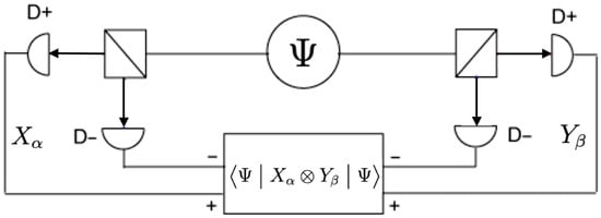
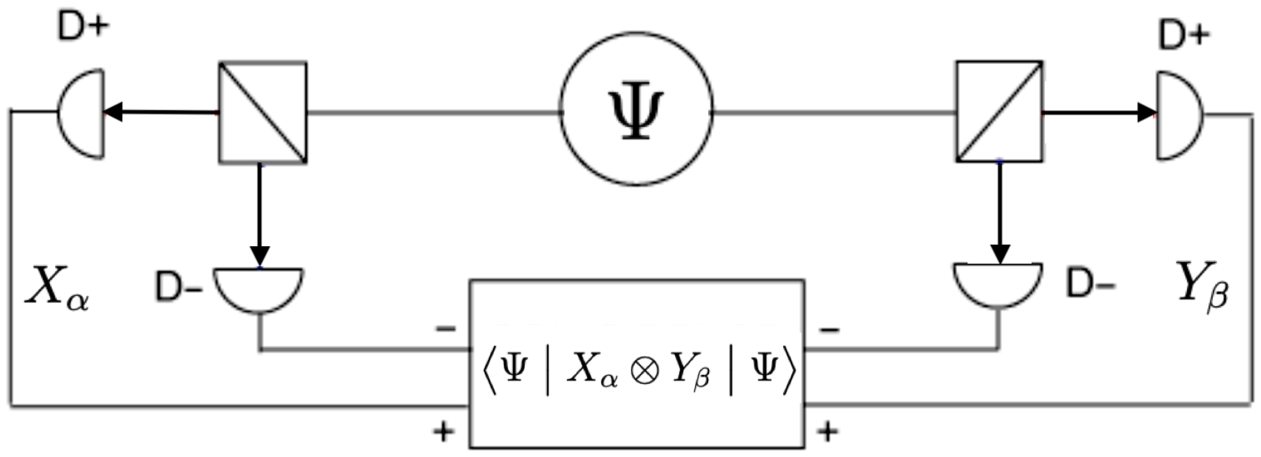
In a quantum mechanical model of the Bell experiment, depicted in Figure 1, there are two detectors, polarimeters, in a line, that we call the y-axis. The detectors measure the spin in the x-z-plane perpendicular to the y-axis. There are two base vectors ${\mathbf{e}}_0={(1,0)}^{\top }$ and ${\mathbf{e}}_1={(0,1)}^{\top }$ used for the spin also known as up and down. The quantum state of an entangled photon pair can be described by

$$\mathbf{\Psi }={\displaystyle \frac{1}{\sqrt{2}}}({\mathbf{e}}_0\otimes {\mathbf{e}}_1-{\mathbf{e}}_1\otimes {\mathbf{e}}_0)\in {\mathbb{C}}^2\otimes {\mathbb{C}}^2.$$

(2)

The polarization is specified by a vector ${\mathbf{f}}_{\theta }={(\cos \left(\theta \right),\sin \left(\theta \right))}^{\top }$ which makes an angle $\theta$ with the x-axis. We define ${\tilde{\mathbf{f}}}_{\theta }:={\mathbf{f}}_{\theta +{\displaystyle \frac{\pi }{2}}}$, so $\widetilde{{\mathbf{f}}_{\theta }}={(-\sin \left(\theta \right),\cos \left(\theta \right))}^{\top }$, which is orthogonal to ${\mathbf{f}}_{\theta }$. The measurement of a photon is done by an observable which could be the projection operator: ${\mathbf{f}}_{\theta }.{\mathbf{f}}_{\theta }^{\top }$. Note that ${\mathbf{f}}_{\theta }.{\mathbf{f}}_{\theta }^{\top }.{\mathbf{f}}_{\theta }={\mathbf{f}}_{\theta }$. So, the eigenvalue is 1 and ${\mathbf{f}}_{\theta }$ is the eigenvector of this projection operator. The only other eigenvalue of this operator is 0 with eigenvector 0. We like to have two non-zero eigenvalues as measurements for the spin up and down. Therefore we transform the projection operator into $2{\mathbf{f}}_{\theta }.{\mathbf{f}}_{\theta }^{\top }-\mathbf{I}$ where $\mathbf{I}$ is the identity operator on the x-z-plane. Now the eigenvalues are 1 and $-1$ with eigenvectors ${\mathbf{f}}_{\theta }$ and $\widetilde{{\mathbf{f}}_{\theta }}$. It is easy to verify that

$$F_{\theta }:={\mathbf{f}}_{\theta }.{\mathbf{f}}_{\theta }^{\top }-{\tilde{\mathbf{f}}}_{\theta }.{\widetilde{{\mathbf{f}}_{\theta }}}^{\top }=2{\mathbf{f}}_{\theta }.{\mathbf{f}}_{\theta }^{\top }-\mathbf{I}$$

(3)

We see that $F_{\theta }:{\mathbb{C}}^2\to {\mathbb{C}}^2$, with $\theta \in [0,\pi )$ is a special type of self-adjoint operator (Hermitean matrix), which is the difference of two orthogonal projections. So, we derived

$$F_{\theta }=\left[\begin{array}{cc}\cos \left(2\theta \right)& \sin \left(2\theta \right)\\ \sin \left(2\theta \right)& -\cos \left(2\theta \right)\end{array}\right],{\mathbf{f}}_{\theta }=\left[\begin{array}{c}\cos \theta \\ \sin \theta \end{array}\right],{\tilde{\mathbf{f}}}_{\theta }={\mathbf{f}}_{\theta +{\displaystyle \frac{\pi }{2}}}=\left[\begin{array}{c}-\sin \theta \\ \cos \theta \end{array}\right].$$

(4)

with eigenvalues (measurements) are $+1$ and $-1$, with respective eigenvectors ${\mathbf{f}}_{\theta }$ and ${\tilde{\mathbf{f}}}_{\theta }$. The CHSH experiment has two detectors, one left $F_{\alpha }$ and one right $F_{\beta }$ and together they form one operator, the observable, modeled by $F_{\alpha }\otimes F_{\beta }$ acting on the entangled state $\mathbf{\Psi }$.

Figure 1. The optical version of the Bell experiment. The entangled photon pair is described by wave function $\mathrm{\Psi }$. The polarimeters $X_{\alpha }$ and $Y_{\beta }$ each comprise a polarizer, with rotatable polarization angles $\alpha$ and $\beta$, and two photon counters labeled D+ and D−. The coincidence monitor $⟨\mathrm{\Psi }|X_{\alpha }\otimes Y_{\beta }|\mathrm{\Psi }⟩$ computes the corresponding quantum mechanical expectation.

In a quantum mechanical model of the Bell experiment the quantum state of an entangled photon pair can be described by

$$\mathbf{\Psi }={\displaystyle \frac{1}{\sqrt{2}}}({\mathbf{e}}_0\otimes {\mathbf{e}}_1-{\mathbf{e}}_1\otimes {\mathbf{e}}_0)\in {\mathbb{C}}^2\otimes {\mathbb{C}}^2.$$

(5)

Here ${\mathbf{e}}_0={(1,0)}^{\top }$ and ${\mathbf{e}}_1={(0,1)}^{\top }$ the two base spin vectors, also known as up and down.

The spin of a photon can be detected by a polarimeter, which is modeled by a special type of self-adjoint operator (Hermitean matrix) $F_{\theta }:{\mathbb{C}}^2\to {\mathbb{C}}^2$,

$$F_{\theta }=\left[\begin{array}{cc}\cos \left(2\theta \right)& \sin \left(2\theta \right)\\ \sin \left(2\theta \right)& -\cos \left(2\theta \right)\end{array}\right],$$

(6)

where $\theta \in [0,\pi )$ is the angle of the polarizer with respect to some reference frame perpendicular to the axis of the experiment. $F_{\theta }$ is the difference of two orthogonal projections

$$F_{\theta }={\mathbf{f}}_{\theta }{\mathbf{f}}_{\theta }^{\top }-{\tilde{\mathbf{f}}}_{\theta }{\tilde{\mathbf{f}}}_{\theta }^{\top },{\mathbf{f}}_{\theta }=\left[\begin{array}{c}\cos \theta \\ \sin \theta \end{array}\right],{\tilde{\mathbf{f}}}_{\theta }={\mathbf{f}}_{\theta +{\displaystyle \frac{\pi }{2}}}=\left[\begin{array}{c}-\sin \theta \\ \cos \theta \end{array}\right].$$

(7)

The outcomes (eigenvalues) of a detection are $+1$ and $-1$, with respective eigenvectors ${\mathbf{f}}_{\theta }$ and ${\tilde{\mathbf{f}}}_{\theta }$. Note that this covers all cases, because ${\mathbf{f}}_{\theta \pm \pi }=-{\mathbf{f}}_{\theta }$.

The CHSH experiment has two detectors $F_{\alpha }$ on the left hand side and $F_{\beta }$ on the right hand side. For later convenience, these are renamed to $X_{\alpha }$ and $Y_{\beta }$ respectively. The outcome of the Bell experiment can now be modeled by $X_{\alpha }\otimes Y_{\beta }$ acting on the entangled state $\mathbf{\Psi }$. For the probability calculations, it is advantageous to orthogonally decompose the entangled state $\mathbf{\Psi }$ according to the spectral resolution of $X_{\alpha }\otimes Y_{\beta }$,

$$\mathbf{\Psi }={\psi }_{1,1}{\mathbf{f}}_{\alpha }\otimes {\mathbf{f}}_{\beta }+{\psi }_{-1,1}{\tilde{\mathbf{f}}}_{\alpha }\otimes {\mathbf{f}}_{\beta }+{\psi }_{1,-1}{\mathbf{f}}_{\alpha }\otimes {\tilde{\mathbf{f}}}_{\beta }+{\psi }_{-1,-1}{\tilde{\mathbf{f}}}_{\alpha }\otimes {\tilde{\mathbf{f}}}_{\beta }.$$

(8)

The coefficients ${\psi }_{xy},x,y\in \{-1,1\}$ are calculated by taking inner products (in Dirac notation). A specimen,

$${\psi }_{-1,1}=⟨\mathbf{\Psi },{\tilde{\mathbf{f}}}_{\alpha }\otimes {\mathbf{f}}_{\beta }{⟩}_{{\mathbb{C}}^2\otimes {\mathbb{C}}^2}.$$

(9)

The probability of the outcome pair $(x,y)$ for detection angles $\alpha$ and $\beta$ is given by Born’s rule

$$p(x,y|\alpha ,\beta )=|{\psi }_{xy}{|}^2.$$

(10)

In Section 5 we will see that this is indeed a conditional probability, given the detector settings. A detailed specimen,

$$\begin{array}{cc}p(-1,1|\alpha ,\beta )=|{\psi }_{-1,1}{|}^2\hfill & ={\displaystyle \frac{1}{2}}{\left(\det \left[\begin{array}{cc}{\mathbf{e}}_0^{\top }{\tilde{\mathbf{f}}}_{\alpha }& {\mathbf{e}}_0^{\top }{\mathbf{f}}_{\beta }\\ {\mathbf{e}}_1^{\top }{\tilde{\mathbf{f}}}_{\alpha }& {\mathbf{e}}_1^{\top }{\mathbf{f}}_{\beta }\end{array}\right]\right)}^2\hfill \\ \hfill & ={\displaystyle \frac{1}{2}}{\left(\det \left[\begin{array}{cc}-\sin \alpha & \cos \beta \\ \cos \alpha & \sin \beta \end{array}\right]\right)}^2={\displaystyle \frac{1}{2}}{\cos }^2(\alpha -\beta ).\hfill \end{array}$$

(11)

In the same way one obtains the following full results:

$$\begin{array}{ccc}p(1,1|\alpha ,\beta )\hfill & =p(-1,-1|\alpha ,\beta )\hfill & ={\displaystyle \frac{1}{2}}{\sin }^2(\alpha -\beta )\hfill \\ p(-1,1|\alpha ,\beta )\hfill & =p(1,-1|\alpha ,\beta )\hfill & ={\displaystyle \frac{1}{2}}{\cos }^2(\alpha -\beta ).\hfill \end{array}$$

(12)

Given these probabilities, the quantum mechanical expectation $⟨X_{\alpha }\otimes Y_{\beta }⟩$ can now be calculated as follows

$$\begin{array}{cc}\hfill & ⟨\mathrm{\Psi }|X_{\alpha }\otimes Y_{\beta }|\mathrm{\Psi }⟩\hfill \\ =\hfill & (1·1)·p(1,1|\alpha ,\beta )+(-1·-1)·p(-1,-1|\alpha ,\beta )+\hfill \\ \hfill & (-1·1)·p(-1,1|\alpha ,\beta )+(1·-1)·p(1,-1|\alpha ,\beta )\hfill \\ =\hfill & {\sin }^2(\alpha -\beta )-{\cos }^2(\alpha -\beta )\hfill \\ =\hfill & -\cos \left(2(\alpha -\beta )\right).\hfill \end{array}$$

(13)

This expectation is in agreement with those of [3,4]. (The minus sign preceding the $\cos \left(\right)$ is sometimes omitted due to different conventions.) Figure 3 in [4] shows an excellent agreement between the measured data and (13).

4. A Model with Four Observables

In nearly all publications on the Bell experiment, including Bell’s, the probability model underlying the experiment is left implicit. That is, they lack a probability model consistent with the standard definitions given in Section 2. These implicit models tacitly assume four stochastic variables (observables) $X_0,X_1,Y_0,Y_1$, corresponding to the four detector settings $a_0,a_1,b_0,b_1$. During a particular experiment only two of them are observed (one X on the left-hand side and one Y on the right-hand side), but the other two are assumed to exist as well. This assumption is sometimes called realism [11]. Note that these the values of the four random variables are in $\{-1,1\}$. The outcome space $\mathrm{\Omega }$ for this experiment is given in Table 1.

Table 1. An outcome space for the CHSH experiment.

	1	2	3	4	5	6	7	8	9	10	11	12	13	14	15	16
$X_0$	−1	1	−1	1	−1	1	−1	1	−1	1	−1	1	−1	1	−1	1
$X_1$	−1	−1	1	1	−1	−1	1	1	−1	−1	1	1	−1	−1	1	1
$Y_0$	−1	−1	−1	−1	1	1	1	1	−1	−1	−1	−1	1	1	1	1
$Y_1$	−1	−1	−1	−1	−1	−1	−1	−1	1	1	1	1	1	1	1	1
CHSH	2	2	−2	−2	−2	2	−2	2	2	−2	2	−2	−2	−2	2	2

The event space $\mathcal{F}$ is the power set of $\mathrm{\Omega }$. We leave the probability measure unspecified, because the arguments we present hold for all possible probabilities measures. It is based on a simple inequality [6]: for $Q,R,S,T\in \{-1,1\}$

$$|QS+QT+RS-RT|\le 2.$$

(14)

This inequality can be generalized to $Q,R,S,T\in [-1,1]$. First we note that

$$|QS+QT+RS-RT|\le \left|Q\right(S+T\left)\right|+\left|R\right(S-T\left)\right|\le |S+T|+|S-T|.$$

(15)

The right-hand side equals $2\left|S\right|$ or $2\left|T\right|$, depending on the four cases of the signs of $S+T$ and $S-T$. So, for these four random variables we have (see last row in Table 1):

$$|X_0{Y}_0+X_1{Y}_0+X_1{Y}_1-X_0{Y}_1|\le 2.$$

(16)

By taking expectations (a linear operation) we obtain

$$|\mathbb{E}\left[X_0{Y}_0\right]+\mathbb{E}\left[X_1{Y}_0\right]+\mathbb{E}\left[X_1{Y}_1\right]-\mathbb{E}\left[X_0{Y}_1\right]|\le 2.$$

(17)

Note that it $\left|\mathbb{E}\right[X_{\alpha }{Y}_{\beta }|\le 1$ and so, for any probability measure on the outcome space of Table 1 Equation (17) holds. Using (13) it follows that

$$\mathbb{E}\left[X_{\alpha }{Y}_{\beta }\right]=⟨\mathrm{\Psi }|X_{\alpha }\otimes Y_{\beta }|\mathrm{\Psi }⟩=⟨X_{\alpha }\otimes Y_{\beta }⟩=-\cos \left(2(\alpha -\beta )\right).$$

(18)

Note that we use here the symbols X and Y for the random variables as well as for the operators X and Y they relate to.

Next, we will use the specific values for the detectors $\alpha :a_0,a_1$ and two for $\beta :b_0,b_1$. (Recall that these settings correspond to the random variables $X_0,X_1,Y_0,Y_1$ as used in Table 1). Following [6],

$$a_0=0,a_1={\displaystyle \frac{1}{4}}\pi ,b_0={\displaystyle \frac{5}{8}}\pi ,b_1={\displaystyle \frac{7}{8}}\pi .$$

(19)

These represent the so-called Tsirelson’s bound [16], where the Bell inequality allegedly is violated most. From (18) it follows that

$$⟨X_0\otimes Y_0⟩=⟨X_1\otimes Y_0⟩=⟨X_1\otimes Y_1⟩=-⟨X_0\otimes Y_1⟩={\displaystyle \frac{1}{2}}\sqrt{2},$$

(20)

which results in

$$|⟨X_0\otimes Y_0⟩+⟨X_1\otimes Y_0⟩+⟨X_1\otimes Y_1⟩-⟨X_0\otimes Y_1⟩|=2\sqrt{2}.$$

(21)

With the assumption

$$\mathbb{E}\left[X_i{Y}_j\right]=⟨X_i\otimes Y_j⟩\mathrm{for}i,j\in \{0,1\}$$

(22)

there is a manifest contradiction between (21) and (17). Our conclusion from this contradiction is that assumption (22) does not hold. More generally, the probability model with four stochastic variables $X_0,X_1,Y_0,Y_1$ does not fit the quantum mechanical model of the experiment. There are only two observables and two detector settings. This means that $⟨X_{\alpha }\otimes Y_{\beta }⟩$ must be a conditional expectation, given the detector settings, as will be explained in the next section.

5. A Model with 2 Observables and 2 Detector Settings

A suitable probability model for the Bell experiment can be based on a different set of four stochastic variables: the two observables X and Y (the two measurements) and the two settings A and B. Furthermore, the quantum mechanical expectation $⟨X_{\alpha }\otimes Y_{\beta }⟩$ now becomes the conditional expectation

$$⟨X_{\alpha }\otimes Y_{\beta }⟩=\mathbb{E}\left[XY|A=\alpha ,B=\beta \right],$$

(23)

that is, the expectation to observe X and Ygiven detector settings A and B. The corresponding (conditional) probability space is shown in Table 2. Note that the outcomes of A and B must be known in order to compute the simultaneous probability of $(X,Y)$. The tabulated probabilities are based on (12), and hence agree with the quantum mechanical model and its experimental validation [4].

Table 2. The conditional probability measure given $A=\alpha ,B=\beta$.

		$\mathit{\alpha }$	A
$\mathit{X}$	$\mathit{Y}$	$\mathit{\beta }$	$\mathit{B}$
1	1	${\displaystyle \frac{1}{2}}{\sin }^2(\alpha -\beta )$
−1	1	${\displaystyle \frac{1}{2}}{\cos }^2(\alpha -\beta )$
1	−1	${\displaystyle \frac{1}{2}}{\cos }^2(\alpha -\beta )$
−1	−1	${\displaystyle \frac{1}{2}}{\sin }^2(\alpha -\beta )$

From Table 2 it can be observed that

$$\begin{array}{ccccc}\mathbb{P}[X=x|A=\alpha ,B=\beta ]\hfill & =\hfill & \mathbb{P}[X=x|A=\alpha ]\hfill & =\hfill & {\displaystyle \frac{1}{2}}\hfill \\ \mathbb{P}[Y=y|A=\alpha ,B=\beta ]\hfill & =\hfill & \mathbb{P}[Y=y|B=\beta ]\hfill & =\hfill & {\displaystyle \frac{1}{2}}.\hfill \end{array}$$

(24)

Clearly, the outcome X does not depend on the setting of detectors A and B. Note that this property holds for all detector settings and for any probability $\mathbb{P}[A=\alpha ,B=\beta ]$.

When we fill in the specific parameters from (19) we obtain Table 3, which depicts the complete probability space: $\mathrm{\Omega }={\{-1,1\}}^2\times \{a_0,a_1\}\times \{b_0,b_1\}$ (a set of 16 cells), $\mathcal{F}$ is the power set of it and $\mathbb{P}[.]$ is represented by the content of the cells. It is easy to verify that $\mathbb{P}[A=a_i,B=b_j]={\displaystyle \frac{1}{4}}$ for $i,j\in \{0,1\}$, which means that A and B are independent.

Table 3. The Bell probability measure for specific detector settings and for all detector combinations the same probability.

		${\mathit{a}}_0$	${\mathit{a}}_1$	${\mathit{a}}_1$	${\mathit{a}}_0$	A
$\mathit{X}$	$\mathit{Y}$	${\mathit{b}}_{\mathbf{0}}$	${\mathit{b}}_{\mathbf{0}}$	${\mathit{b}}_{\mathbf{1}}$	${\mathit{b}}_{\mathbf{1}}$	$\mathit{B}$
1	1	${\gamma }^2/8$	${\gamma }^2/8$	${\gamma }^2/8$	${\beta }^2/8$
−1	1	${\beta }^2/8$	${\beta }^2/8$	${\beta }^2/8$	${\gamma }^2/8$	${\beta }^2={\sin }^2\left({\displaystyle \frac{\pi }{8}}\right)={\displaystyle \frac{1}{4}}(2-\sqrt{2})$
1	−1	${\beta }^2/8$	${\beta }^2/8$	${\beta }^2/8$	${\gamma }^2/8$	${\gamma }^2={\cos }^2\left({\displaystyle \frac{\pi }{8}}\right)={\displaystyle \frac{1}{4}}(2+\sqrt{2})$
−1	−1	${\gamma }^2/8$	${\gamma }^2/8$	${\gamma }^2/8$	${\beta }^2/8$

Note that the first three columns are identical, because ${\sin }^2(0-{\displaystyle \frac{5}{8}}\pi )={\sin }^2({\displaystyle \frac{1}{4}}\pi -{\displaystyle \frac{5}{8}}\pi )={\sin }^2({\displaystyle \frac{1}{4}}\pi -{\displaystyle \frac{7}{8}}\pi )={\cos }^2\left({\displaystyle \frac{1}{8}}\pi \right)={\gamma }^2$. Similarly, we derive for $(i,j)\in \left\{\right(0,0),(1,0),(1,1\left)\right\}$:

$$\begin{array}{ccccc}\mathbb{E}\left[XY\right|A=a_i,B=b_j]=-\cos \left(2(a_i-b_j)\right)\hfill & =\hfill & \hfill \cos \left({\displaystyle \frac{1}{4}}\pi \right)& \hfill =& \hfill {\displaystyle \frac{1}{2}}\sqrt{(}2).,\\ \mathbb{E}\left[XY\right|A=a_0,B=b_1]\hfill & =\hfill & \hfill -\cos \left({\displaystyle \frac{1}{4}}\pi \right)& \hfill =& \hfill -{\displaystyle \frac{1}{2}}\sqrt{(}2).\end{array}$$

(25)

So, this is consistent with (20) and (21) and therefore we don’t have a contradiction. The step from (16) to (17) is allowed for expectations, but is incorrect for conditional expectations under different conditions. This is the cause of the earlier contradiction. Aside: conditional expectations looks like a simple and innocent operation: $\mathbb{E}[X+Y|H_1]=\mathbb{E}\left[X\right|H_2]+\mathbb{E}\left[Y\right|H_3]$, is only true if $H_1=H_2=H_3$. As an example consider the sum of dice X and Y. With $\mathbb{E}\left[X\right]=\mathbb{E}\left[Y\right]=3.5$ it follows that $\mathbb{E}[X+Y]=7$. However, $\mathbb{E}[X+Y|X=Y]=\mathbb{E}[X+Y|X\ne Y]=7$. Therefore, $\mathbb{E}[X+Y]\ne \mathbb{E}[X+Y|X=Y]+\mathbb{E}[X+Y|X\ne Y]$.

We will explain this contradiction in a different way. Define, for each $\alpha$ and $\beta$, new random variables:

$$\begin{array}{ccc}{\tilde{X}}_{\alpha }\hfill & :=\hfill & X·{\mathbf{1}}_{\{A=\alpha \}}\hfill \\ {\tilde{Y}}_{\beta }\hfill & :=\hfill & Y·{\mathbf{1}}_{\{B=\beta \}}.\hfill \end{array}$$

(26)

It is easy to verify that:

$$\begin{array}{ccc}\mathbb{E}\left[{\tilde{X}}_{\alpha }{\tilde{Y}}_{\beta }\right]\hfill & =\hfill & \sum _{x,y}x·y·\mathbb{P}[X=x,Y=y,A=\alpha ,B=\beta ]\hfill \\ \hfill & =\hfill & \sum _{x,y}x·y·\mathbb{P}[X=x,Y=y|A=\alpha ,B=\beta ]·\mathbb{P}[A=\alpha ,B=\beta ]\hfill \\ \hfill & =\hfill & \mathbb{E}\left[XY\right|A=\alpha ,B=\beta ]·\mathbb{P}[A=\alpha ,B=\beta ]\hfill \\ \hfill & =\hfill & ⟨X_{\alpha }\otimes Y_{\beta }⟩·\mathbb{P}[A=\alpha ,B=\beta ]\hfill \end{array}$$

(27)

If we take the four Tsirelson’s angles (19) for $\alpha$ and $\beta$ and we assume $\mathbb{P}[A=\alpha ,B=\beta ]={\displaystyle \frac{1}{4}}$ then we obtain

$$\begin{array}{cc}\hfill & |\mathbb{E}\left[{\tilde{X}}_0{\tilde{Y}}_0\right]+\mathbb{E}\left[{\tilde{X}}_1{\tilde{Y}}_0\right]+\mathbb{E}\left[{\tilde{X}}_1{\tilde{Y}}_1\right]-\mathbb{E}\left[{\tilde{X}}_0{\tilde{Y}}_1\right]|\hfill \\ =\hfill & {\displaystyle \frac{1}{4}}|⟨X_0\otimes Y_0⟩+⟨X_1\otimes Y_0⟩+⟨X_1\otimes Y_1⟩-⟨X_0\otimes Y_1⟩|\hfill \\ =\hfill & {\displaystyle \frac{1}{2}}\sqrt{2}\le 2\hfill \end{array}$$

(28)

So, there is no contradiction with the four observables ${\tilde{X}}_0,{\tilde{X}}_1,{\tilde{Y}}_0,{\tilde{Y}}_1$. But note that they are only different from 0 if the settings are correct.

Empirically, one has to estimate $\mathbb{E}[{\tilde{X}}_{\alpha }{\tilde{Y}}_{\beta }]$, which can be done by application of the law of large numbers:

$$\mathbb{E}[{\tilde{X}}_{\alpha }{\tilde{Y}}_{\beta }]=\underset{N\to \infty }{\lim }{\displaystyle \frac{1}{N}}\sum _{n=0}^{N-1}{X}^{\left(n\right)}·Y^{\left(n\right)}·{\mathbf{1}}_{\{A=\alpha ,B=\beta \}},$$

(29)

where $X^{\left(n\right)}$ is an independent copy of X and similarly $Y^{\left(n\right)}$ of Y. Most likely, experimenters have computed:

$$\mathbb{E}\left[XY\right|A=\alpha ,B=\beta ]=\underset{N\to \infty }{\lim }{\displaystyle \frac{1}{M}}\sum _{n=0}^{N-1}{X}^{\left(n\right)}·Y^{\left(n\right)}·{\mathbf{1}}_{\{A=\alpha ,B=\beta \}},$$

(30)

where

$$M:=\sum _{n=0}^{N-1}{\mathbf{1}}_{\{A=\alpha ,B=\beta \}},$$

(31)

because it is more natural to take averages over the outcomes per setting. This suggests that the experimental outcomes of $⟨X_{\alpha }\otimes Y_{\beta }⟩$ correspond to conditional expectations, which explains the contradiction. Below this model will be referred to as the 2-observables model.

6. The 2-Observables Model Extended with Hidden Variables

Following [1], we extend the proposed probability model with a hidden variable. In order to accommodate this hidden variable, the outcome space for the Bell experiment is extended with a random variable $\in \mathrm{\Lambda }$, which is assumed here to be at most countable.

$$\mathrm{\Omega }={\{-1,1\}}^2\times \{a_0,a_1\}\times \{b_0,b_1\}\times \mathrm{\Lambda }.$$

(32)

Let random variable L denote the hidden variable with $L\left(\omega \right)=\lambda$ for $\omega =(x,y,\alpha ,\beta ,\lambda )$. The probability measure of this extended model must be consistent with Table 2 and hence must satisfy

$$\begin{array}{ccc}\hfill & \hfill & \mathbb{P}[X=x,Y=y|A=a,B=b]\hfill \\ \hfill & =\hfill & \sum _{\lambda \in \mathrm{\Lambda }}\mathbb{P}[X=x,Y=y|A=a,B=b,L=\lambda ]·\mathbb{P}[A=a,B=b,L=\lambda ].\hfill \end{array}$$

(33)

Critically, L must be independent of the detector settings A and B. This assumption is known as statistical independence or measurement independence [9]:

$$\mathbb{P}[A=a,B=b,L=\lambda ]=\mathbb{P}[A=a,B=b]·\mathbb{P}[L=\lambda ].$$

(34)

This assumption is consistent with the idea that $\lambda$ is given before A and B are selected. In this section we prove:

1.

This extended probability model is non-separable.

2.

The non-separability of the model implies that it is non-deterministic or non-local (or both).

These properties are according to established definitions.

6.1. Statistical Locality

With (24) we observed that the outcome X does not depend on the setting of detectors A and B, and likewise for outcome Y. The property of (statistical) locality [9] is defined by

$$\begin{array}{ccc}\mathbb{P}[X=x|A=\alpha ,B=\beta ,L=\lambda ]\hfill & =\hfill & \mathbb{P}[X=x|A=\alpha ,L=\lambda ]\hfill \\ \mathbb{P}[Y=y|A=\alpha ,B=\beta ,L=\lambda ]\hfill & =\hfill & \mathbb{P}[Y=y|B=\beta ,L=\lambda ].\hfill \end{array}$$

(35)

Note that this must hold for all $\alpha ,\beta ,\lambda$. Paraphrasing [9]: “Thus, an observer cannot distinguish, via any local measurement based on detector setting A, whether a distant observer has carried out measurement using detector setting B or $B^{\prime }$), even given knowledge of the underlying variable $\lambda$. This property, also known as parameter independence and as no-signalling [8], is justified by the principle of relativity when the measurement subprocedures are carried out in spacelike separated regions [1].” Statistical locality is not assumed a priori to be a property for the extended model including hidden variable.

6.2. Bell Separability

The probability model including a hidden variable, is separable [1,9] if, for all $x,y,\alpha ,\beta$:

$$\begin{array}{ccc}p(x,y|\alpha ,\beta )\hfill & =\hfill & \sum _{\lambda \in \mathrm{\Lambda }}{p}_1\left(x\right|\alpha ,\lambda )·p_2\left(y\right|\beta ,\lambda )·\rho \left(\lambda \right)\hfill \\ p_1\left(x\right|\alpha ,\lambda )\hfill & :=\hfill & \mathbb{P}[X=x|A=\alpha ,L=\lambda ]\hfill \\ p_2\left(y\right|\beta ,\lambda )\hfill & :=\hfill & \mathbb{P}[Y=y|B=\beta ,L=\lambda ],\hfill \end{array}$$

(36)

where $p(x,y|\alpha ,\beta )$ is used as a shorthand for $\mathbb{P}[X=x,Y=y|A=\alpha ,B=\beta ]$, and $\rho \left(\lambda \right)$ is a shorthand for $\mathbb{P}[L=\lambda ]$. The extended probability measure is repeated in Table 4, including an assumed factorization given hidden variable $\lambda$.

Table 4. The conditional probability measure, given detector settings $\alpha ,\beta$ (column $\alpha \beta$), and an assumed factorization given hidden variable $\lambda$ (column $\alpha \beta \lambda$).

		$\mathit{\alpha }$	$\mathit{\alpha }$	A
		$\mathit{\beta }$	$\mathit{\beta }$	$\mathit{B}$
$\mathit{X}$	$\mathit{Y}$		$\mathit{\lambda }$	$\mathit{L}$
1	1	${\displaystyle \frac{1}{2}}{\sin }^2(\alpha -\beta )$	$p_1\left(1\right|\alpha ,\lambda )$·$p_2\left(1\right|\beta ,\lambda )$
−1	1	${\displaystyle \frac{1}{2}}{\cos }^2(\alpha -\beta )$	$(1-p_1\left(1\right|\alpha ,\lambda ))$·$p_2\left(1\right|\beta ,\lambda )$
1	−1	${\displaystyle \frac{1}{2}}{\cos }^2(\alpha -\beta )$	$p_1\left(1\right|\alpha ,\lambda )$·$(1-p_2\left(1\right|\beta ,\lambda ))$
−1	−1	${\displaystyle \frac{1}{2}}{\sin }^2(\alpha -\beta )$	$(1-p_1\left(1\right|\alpha ,\lambda ))$·$(1-p_2\left(1\right|\beta ,\lambda ))$

Separability, for $\alpha =\beta$ would imply

$$\begin{array}{ccc}\sum _{\lambda \in \mathrm{\Lambda }}{p}_1\left(1\right|\alpha ,\lambda )·p_2\left(1\right|\alpha ,\lambda ))\rho \left(\lambda \right)\hfill & =\hfill & 0\hfill \\ \sum _{\lambda \in \mathrm{\Lambda }}(1-p_1\left(1\right|\alpha ,\lambda ))·(1-p_2\left(1\right|\alpha ,\lambda ))\rho \left(\lambda \right)\hfill & =\hfill & 0.\hfill \end{array}$$

(37)

Hence, $1-p_1\left(1\right|\alpha ,\lambda )-p_2\left(1\right|\alpha ,\lambda )=0$ for all $\lambda \in \mathrm{\Lambda }$, with $\rho \left(\lambda \right)>0$. Substitution of $p_2\left(1\right|\alpha ,\lambda )=1-p_1\left(1\right|\alpha ,\lambda )$ in (37) gives

$$\sum _{\lambda \in \mathrm{\Lambda }}{p}_1\left(1\right|\alpha ,\lambda )·(1-p_1\left(1\right|\alpha ,\lambda ))\rho \left(\lambda \right)=0.$$

(38)

This constraint on $p_1$ can be rephrased as

$$p_1\left(x\right|\alpha ,\lambda )\in \{0,1\}{p}_2\left(y\right|\beta ,\lambda )\in \{0,1\}.$$

(39)

This property relates to (non-)determinism, which is the topic of Section 6.3.

If Bell separability holds, we derive:

$$\sum _{x,y}x·y·p(x,y|\alpha ,\beta )=\sum _{\lambda \in \mathrm{\Lambda }}\left(\sum _{x}x·p_1\left(x\right|\alpha ,\lambda )·\sum _{y}y·p_2\left(y\right|\beta ,\lambda )\right)·\rho \left(\lambda \right),$$

(40)

or, equivalently,

$$\mathbb{E}\left[XY\right|A=\alpha ,B=\beta ]=\sum _{\lambda \in \mathrm{\Lambda }}\mathbb{E}\left[X\right|A=\alpha ,L=\lambda ]·\mathbb{E}\left[Y\right|B=\beta ,L=\lambda ]·\rho \left(\lambda \right).$$

(41)

Next, by choosing the elements $a_0,a_1,b_0,b_1$ equal to Tsirelson’s angles (19) and we define

$$\begin{array}{ccc}{Q}_{\lambda }\hfill & :=\hfill & \mathbb{E}\left[X\right|A=a_0,L=\lambda ]\hfill \\ R_{\lambda }\hfill & :=\hfill & \mathbb{E}\left[X\right|A=a_1,L=\lambda ]\hfill \\ S_{\lambda }\hfill & :=\hfill & \mathbb{E}\left[Y\right|B=b_0,L=\lambda ]\hfill \\ T_{\lambda }\hfill & :=\hfill & \mathbb{E}\left[Y\right|B=b_1,L=\lambda ].\hfill \end{array}$$

(42)

Note that $Q_{\lambda },R_{\lambda },T_{\lambda },$ and $S_{\lambda },$ are all in $[-1,1]$. Their substitution in (41) results in.

$$\begin{array}{ccc}\mathbb{E}\left[XY\right|A=a_0,B=b_0]\hfill & =\hfill & \sum _{\lambda }{Q}_{\lambda }{S}_{\lambda }\rho \left(\lambda \right)\hfill \\ \mathbb{E}\left[XY\right|A=a_0,B=b_1]\hfill & =\hfill & \sum _{\lambda }{Q}_{\lambda }{T}_{\lambda }\rho \left(\lambda \right)\hfill \\ \mathbb{E}\left[XY\right|A=a_1,B=b_1]\hfill & =\hfill & \sum _{\lambda }{R}_{\lambda }{S}_{\lambda }\rho \left(\lambda \right)\hfill \\ \mathbb{E}\left[XY\right|A=a_1,B=b_1]\hfill & =\hfill & \sum _{\lambda }{R}_{\lambda }{T}_{\lambda }\rho \left(\lambda \right).\hfill \end{array}$$

(43)

By (25) we have

$$\mathbb{E}\left[XY\right|A=a_0,B=b_0]={\displaystyle \frac{1}{2}}\sqrt{2},$$

(44)

and similar for the others. So, on the one hand

$$\begin{array}{cccc}\hfill & \mathbb{E}\left[XY\right|A=a_0,B=b_0]\hfill & +\hfill & \mathbb{E}\left[XY\right|A=a_0,B=b_1]\hfill \\ +\hfill & \mathbb{E}\left[XY\right|A=a_1,B=b_1]\hfill & -\hfill & \mathbb{E}\left[XY\right|A=a_0,B=b_1])=2\sqrt{2},\hfill \end{array}$$

(45)

and on the other hand the left-hand side of (45) equals:

$$\sum _{\lambda }\left(Q_{\lambda }{S}_{\lambda }+R_{\lambda }{T}_{\lambda }+R_{\lambda }{S}_{\lambda }-Q_{\lambda }{T}_{\lambda }\right)·\rho \left(\lambda \right).$$

(46)

By the CHSH inequality (14) for each $\lambda \in \mathrm{\Lambda }$:

$$|Q_{\lambda }{S}_{\lambda }+R_{\lambda }{T}_{\lambda }+R_{\lambda }{S}_{\lambda }-Q_{\lambda }{T}_{\lambda }|\le 2.$$

(47)

And therefore:

$$\sum _{\lambda \in \mathrm{\Lambda }}\left(Q_{\lambda }{S}_{\lambda }+R_{\lambda }{T}_{\lambda }+R_{\lambda }{S}_{\lambda }-Q_{\lambda }{T}_{\lambda }\right)·\rho \left(\lambda \right)\le 2.$$

(48)

Equation (45) is in clear contradiction with (48). This contradiction proves that the probability measure is not Bell separable. This proof is a formalization of a sketch offered by [8]. An alternative proof without the use of the CHSH-inequality is given in Appendix A. In summary we conclude that there does not exist a hidden variable that makes our probability measure separable. Note that we did not assume any structure of the hidden variable, except measurement independence (34).

6.3. Determinism

The model is called deterministic if for all $\lambda \in \mathrm{\Lambda }$ [9]

$$\mathbb{P}[X=x,Y=y|A=a,B=b,L=\lambda ]\in \{0,1\}.$$

(49)

For a model that is (statistically) local (35), Bell separability (36) is equivalent to determinism:

$$\mathcal{S}\wedge \mathcal{L}\iff \mathcal{D}\wedge \mathcal{L},$$

(50)

where $\mathcal{S},\mathcal{L}$, and $\mathcal{D}$ denote the properties separable, statistically local, and deterministic, respectively. The immediate implication is

$$\neg \mathcal{S}\Rightarrow \neg \mathcal{D}\vee \neg \mathcal{L}.$$

(51)

In words, the proposed probability model is not separable, and therefore it is non-deterministic or non-local (or both).

The proof of (50) is presented in two parts. First we focus on $\mathcal{S}\wedge \mathcal{L}\Rightarrow \mathcal{D}$, which makes use of the following lemma.

$$\begin{array}{cc}\hfill & p_1\left(x\right|\alpha ,\beta ,\lambda )\in \{0,1\}\wedge p_2\left(y\right|\alpha ,\beta ,\lambda )\in \{0,1\}\hfill \\ \Rightarrow \hfill & p(x,y|\alpha ,\beta ,\lambda )=p_1\left(x\right|\alpha ,\beta ,\lambda )·p_2\left(y\right|\alpha ,\beta ,\lambda )\in \{0,1\},\hfill \end{array}$$

(52)

where p, $p_1$, and $p_2$ are obvious generalizations of those in (36). From $p_1\left(\right)$ we conclude that for only one x we have $p_1\left(x\right|\alpha ,\beta ,\lambda )\ne 0$ and similarly for $p_2\left(\right)$. Hence, for only one pair $x,y$ it holds that $p(x,y|\alpha ,\beta ,\lambda )\ne 0$. For that pair the probability must be 1.

Given this lemma, we prove $\mathcal{S}\wedge \mathcal{L}\Rightarrow \mathcal{D}$ by

$$\begin{array}{cc}\hfill & \mathcal{S}\wedge \mathcal{L}\hfill \\ \Rightarrow \hfill & \left\{\mathrm{Property}\right(39\left)\right\}\hfill \\ \hfill & p_1\left(x\right|\alpha ,\lambda )\in \{0,1\}\wedge p_2\left(y\right|\beta ,\lambda )\in \{0,1\}\wedge \mathcal{L}\hfill \\ \Rightarrow \hfill & \{\mathrm{Definition}\mathcal{L},(35\left)\right\}\hfill \\ \hfill & p_1\left(x\right|\alpha ,\beta ,\lambda )\in \{0,1\}\wedge p_2\left(y\right|\alpha ,\beta ,\lambda )\in \{0,1\}\hfill \\ \Rightarrow \hfill & \left\{\mathrm{Property}\right(52\left)\right\}\hfill \\ \hfill & p(x,y|\alpha ,\beta ,\lambda )\in \{0,1\}\hfill \\ =\hfill & \{\mathrm{Definition}\mathcal{D},(49\left)\right\}\hfill \\ \hfill & \mathcal{D}.\hfill \end{array}$$

(53)

The second part of the proof makes use of a similar lemma.

$$\begin{array}{cc}\hfill & p(x,y|\alpha ,\beta ,\lambda )\in \{0,1\}\hfill \\ \Rightarrow \hfill & p_1\left(x\right|\alpha ,\beta ,\lambda )\in \{0,1\}\wedge p_2\left(y\right|\alpha ,\beta ,\lambda )\in \{0,1\}\hfill \\ \hfill & \wedge p(x,y|\alpha ,\beta ,\lambda )=p_1\left(x\right|\alpha ,\beta ,\lambda )·p_2\left(y\right|\alpha ,\beta ,\lambda ),\hfill \end{array}$$

(54)

because there can be only one $x,y$ for which $p(x,y|\alpha ,\beta ,\lambda )=1$.

Given this lemma, we prove $\mathcal{D}\wedge \mathcal{L}\Rightarrow \mathcal{S}$ by

$$\begin{array}{cc}\hfill & p(x,y|\alpha ,\beta )\mathrm{assume}\mathcal{D}\wedge \mathcal{L}\hfill \\ =\hfill & \left\{\mathrm{Probability}\mathrm{theory}\mathrm{and}\mathrm{measurement}\mathrm{independence}\right(34\left)\right\}\hfill \\ \hfill & \sum _{\lambda \in \mathrm{\Lambda }}p(x,y|\alpha ,\beta ,\lambda )·\rho \left(\lambda \right)\mathrm{assume}\mathcal{D}\wedge \mathcal{L}\hfill \\ =\hfill & \left\{\mathrm{Property}\right(54\left),\mathrm{given}\mathcal{D}\right\}\hfill \\ \hfill & \sum _{\lambda \in \mathrm{\Lambda }}{p}_1\left(x\right|\alpha ,\beta ,\lambda )·p_2\left(y\right|\alpha ,\beta ,\lambda )·\rho \left(\lambda \right)\mathrm{assume}\mathcal{L}\hfill \\ =\hfill & \{\mathrm{Definition}\mathcal{L},(35\left)\right\}\hfill \\ \hfill & \sum _{\lambda \in \mathrm{\Lambda }}{p}_1\left(x\right|\alpha ,\lambda )·p_2\left(y\right|\beta ,\lambda )·\rho \left(\lambda \right).\hfill \end{array}$$

(55)

That is, given $\mathcal{D}\wedge \mathcal{L}$, the probability model is Bell-separable (36).

7. Conclusions

This paper proposes a probability model for the Bell experiment. The outcome space is defined as the cartesian product space of random variables A and B (detector settings) and X and Y, the corresponding measurement outcomes. It has only two simultaneously observable detector settings per measurement and therefore does not need the assumption of realism. The probability measure $p(x,y,a,b)$ is derived from quantum mechanics and described by Table 2 and Table 3.

From this probability measure it follows that the conditional expectation $\mathbb{E}[X·Y|A=\alpha ,B=\beta ]$ corresponds to Born expectation $⟨X_{\alpha }\otimes Y_{\beta }⟩$. The Bell contradiction arises from the summation of conditional expectations with different conditions (i.e., different detector settings). The 2-observables model (Section 5) does not show such a contradiction. The experimental results by Aspect et al. [4] are “in excellent agreement with the quantum mechanical predictions” and therefore also with the proposed model.

In Section 6 we extend the probability model with a hidden variable. This extended probability model is proved to be non-separable in the Bell sense. (The proof in Section 6.2 makes use of the CHSH inequality. The alternative proof in Appendix A does not.) This non-separability of the probability measure supports Bell’s [17] conclusion “If [a hidden-variable theory] is local it will not agree with quantum mechanics, and if it agrees with quantum mechanics it will not be local”. Furthermore, non-separability implies that the model is non-deterministic or non-local (or both).

References

- Bell, J.S. On the Einstein Podolsky Rosen paradox. Physics 1964, 1, 195–200. [Google Scholar] [CrossRef] [Scilit]
- Einstein, A.; Podolsky, B.; Rosen, N. Can Quantum-Mechanical Description of Physical Reality Be Considered Complete? Phys. Rev. 1935, 47, 777–780. [Google Scholar] [CrossRef] [Scilit]
- Clauser, J.F.; Horne, M.A.; Shimony, A.; Holt, R.A. Proposed Experiment to Test Local Hidden-Variable Theories. Phys. Rev. Lett. 1969, 23, 880–884. [Google Scholar] [CrossRef] [Scilit]
- Aspect, A.; Dalibard, J.; Roger, G. Experimental Test of Bell’s Inequalities Using Time-Varying Analyzers. Phys. Rev. Lett. 1982, 49, 1804–1807. [Google Scholar] [CrossRef] [Scilit]
- Hensen, B.; Bernien, H.; Dréau, A.; Reiserer, A.; Kalb, N.; Blok, M.S.; Ruitenberg, J.; Vermeulen, R.F.L.; Schouten, R.N.; Abellán, C.; et al. Loophole-free Bell inequality violation using electron spins separated by 1.3 kilometres. Nature 2015, 526, 682–686. [Google Scholar] [CrossRef] [Scilit] [PubMed]
- Nielsen, M.A.; Chuang, I.L. Quantum Computation and Quantum Information; Cambridge University Press: Cambridge, UK, 2000. [Google Scholar]
- Gill, R.D. Statistics, Causality and Bell’s Theorem. Stat. Sci. 2014, 29, 512–528. [Google Scholar] [CrossRef] [Scilit]
- Brunner, N.; Cavalcanti, D.; Pironio, S.; Scarani, V.; Wehner, S. Bell nonlocality. Rev. Mod. Phys. 2014, 86, 419–478. [Google Scholar] [CrossRef] [Scilit]
- Hall, M.J.W. The Significance of Measurement Independence for Bell Inequalities and Locality. In At the Frontier of Spacetime; Springer: Berlin/Heidelberg, Germany, 2015. [Google Scholar] [CrossRef] [Scilit]
- Chaves, R.; Cavalcanti, D.; Aolita, L. Causal hierarchy of multipartite Bell nonlocality. Quantum 2017, 1, 23. [Google Scholar] [CrossRef] [Scilit]
- Gill, R.D. Comment on “Bell’s Theorem Versus Local Realism in a Quaternionic Model of Physical Space”. IEEE Access 2021, 9, 154933–154937. [Google Scholar] [CrossRef] [Scilit]
- Kolmogorov, A.N. Grundbegriffe der Wahrscheinlichkeitsrechnung; Springer: Berlin/Heidelberg, Germany, 1933. [Google Scholar]
- Kolmogorov, A.N. Foundations of the Theory of Probability, 2nd ed.; Chelsea: New York, NY, USA, 1950. [Google Scholar]
- Feller, W. An Introduction to Probability Theory and Its Applications; Wiley: Hoboken, NJ, USA, 1968; Volume 1. [Google Scholar]
- Wikipedia Contributors. Probability Space—Wikipedia, The Free Encyclopedia. 2023. Available online: https://en.wikipedia.org/wiki/Probability_space (accessed on 3 January 2023).
- Pál, K.F.; Vértesi, T. Platonic Bell inequalities for all dimensions. Quantum 2022, 6, 756. [Google Scholar] [CrossRef] [Scilit]
- Bell, J.S.; Aspect, A. Speakable and Unspeakable in Quantum Mechanics: Collected Papers on Quantum Philosophy, 2nd ed.; Cambridge University Press: Cambridge, UK, 2004. [Google Scholar] [CrossRef] [Scilit]
Disclaimer/Publisher’s Note: The statements, opinions and data contained in all publications are solely those of the individual author(s) and contributor(s) and not of MDPI and/or the editor(s). MDPI and/or the editor(s) disclaim responsibility for any injury to people or property resulting from any ideas, methods, instructions or products referred to in the content. |
© 2026 by the authors. Licensee MDPI, Basel, Switzerland. This article is an open access article distributed under the terms and conditions of the Creative Commons Attribution (CC BY) license.