Physics-Informed Predictive Energy Management Strategy for HEVs Using Kalman-Enhanced Transformer

Abstract

Predictive energy management strategies (PEMSs) have attracted increasing attention in hybrid electric vehicles (HEVs) for improving fuel economy and powertrain efficiency using anticipated driving information. For PEMS, data-driven velocity prediction is widely used to capture complex driving patterns from historical trajectories and future traffic priors, but often lacks kinematic awareness, leading to physical causality violations and long-horizon state drift. To address these issues, this paper proposes a physics-informed PEMS, where a Physics-Informed Spatio-Temporal Network (PI-STN) provides control-oriented velocity information for an MPC-based energy management controller. Specifically, to address pseudo-motion in velocity prediction under standstill conditions, a global zero-speed gating mechanism is introduced; to suppress acceleration/deceleration trends that violate vehicle kinematic causality, a causal penalty is designed; and to mitigate temporal phase misalignment between data-driven predictions and physical motion priors, a Differentiable Kalman Filter (DKF) is incorporated. At each receding horizon step, the PI-STN-predicted velocity sequence is converted into future power demand through longitudinal vehicle dynamics and used by MPC for engine–battery power allocation under SOC and engine transient constraints. Under the same tested conditions, the proposed strategy reduces engine power fluctuation by 15.1% compared with BiLSTM-Transformer, and achieves an equivalent fuel consumption of 323.74 g, outperforming Transformer-KF by 3.12%.

1. Introduction

Faced with increasingly severe energy and environmental challenges, hybrid electric vehicles (HEVs), owing to their favorable fuel economy and extended driving range, are playing an increasingly important role in the low-carbon transformation of the automotive industry [1,2]. In HEV powertrain systems, effective energy management plays an important role in coordinating power delivery between the engine and the motor, thereby influencing overall vehicle efficiency [3,4]. More broadly, energy management has also been investigated in other electromechanical energy conversion systems, such as turbine-driven power systems and self-powered dynamic systems, where coordinated power-flow control is essential for improving operating efficiency and system stability [5,6]. However, compared with these relatively stationary energy conversion platforms, HEV energy management faces stronger coupling with stochastic driving behavior, transient power demand, and battery SOC constraints. In many HEV applications, however, energy management decisions still mainly rely on the current vehicle state, which may limit the utilization of forthcoming traffic and road information.

In recent years, with the rapid development of Vehicle-to-Everything (V2X), 5G communications, and intelligent transportation systems, vehicles have become increasingly capable of acquiring prior information such as upcoming road conditions, traffic flow states, and traffic signal timing. As a result, predictive energy management strategies have attracted growing research interest [7,8]. Against this background, Model Predictive Control (MPC) has emerged as a promising underlying energy allocator because it can explicitly handle multivariable physical constraints and perform rolling optimization over a finite prediction horizon [9,10]. However, the effectiveness of MPC depends heavily on the accuracy of upper-layer predictions of future driving trajectories. Prediction errors may degrade optimization performance and, in some cases, lead to inappropriate control actions such as battery overcharging or overdischarging. Therefore, developing a high-fidelity and robust vehicle velocity prediction model is an important requirement for predictive energy management systems [11,12].

Early research primarily relied on stochastic theories and statistical methods. For instance, Kong et al. [13] proposed a variable-horizon predictive energy management strategy in which an integrated velocity predictor combines a Markov model with speed-limit information, demonstrating the importance of prediction horizon design and future traffic information for improving predictive energy management performance. S. Lefèvre et al. [14] compared hidden Markov models with Gaussian processes, highlighting the advantages of nonparametric methods in capturing traffic uncertainties. However, traditional statistical models exhibit limitations in representational capacity under long prediction horizons and highly complex, nonlinear driving conditions. With the rise of artificial intelligence, data-driven deep learning models have been increasingly adopted: Tao Li et al. [15] proposed a velocity prediction model based on a Bidirectional Long Short-Term Memory network (Bi-LSTM), and the results showed improved prediction accuracy and adaptability under unknown real-world road conditions; H. Shen et al. [16] proposed a hybrid deterministic-stochastic prediction framework using a Transformer to extract macroscopic sequence features, effectively improving the reliability of energy consumption estimation for electric vehicles; Jingda Wu et al. [17] further incorporated surrounding traffic flow information and proposed a predictive energy management strategy based on a self-attention mechanism, showing that this model improved prediction accuracy by 5.3% compared to traditional methods relying solely on ego-vehicle historical data; moreover, Dong Xiao et al. [18] developed a Hybrid Kalman Recurrent Neural Network (Hybrid Kalman RNN) for trajectory prediction, with experimental results indicating that combining kinematic models with neural networks can effectively smooth predicted trajectories. However, such hybrid designs do not necessarily ensure that physical priors are embedded into a fully differentiable and control-oriented optimization process. Overall, data-driven velocity prediction methods have been continuously refined, and their performance on numerical metrics such as Root Mean Square Error (RMSE) and Mean Absolute Error (MAE) has continued to improve.

However, in the practical application of MPC for HEVs, these data-driven models may still face an important challenge: high prediction accuracy does not always translate into improved control performance. One possible reason is that purely data-driven frameworks are often trained to minimize numerical prediction errors in Euclidean space, whereas actual vehicle motion is constrained by nonlinear kinematic mechanisms.

This mismatch may appear in both spatial and temporal dimensions. First, physical boundaries and causal relationships may not be adequately respected. Without explicit awareness of underlying constraints, deep neural networks may produce abnormal acceleration or deceleration behaviors beyond feasible dynamic limits, and may even generate high-frequency non-physical pseudo-motion disturbances during zero-speed idling. Second, temporal phase lag may occur. When drastic transient load changes such as hard braking or rapid acceleration take place, autoregressive temporal models tend to produce overly smoothed mean predictions, resulting in accumulated errors and delayed tracking responses.

More importantly, because MPC relies on the derivative of velocity to estimate future power demand, the high-frequency non-physical fluctuations in the predicted velocity sequence and the phase lag in the temporal dimension can be further amplified by the controller’s internal differential operations. This differential amplification effect may trigger high-frequency fluctuations in power commands, causing the engine to deviate more frequently from its optimal operating line (OOL) and operate in less efficient regions. As a result, achieving a good balance between fuel economy and powertrain operational smoothness may become more difficult. From this perspective, this paper argues that, in predictive energy management, the control-oriented quality of predicted information may be more important than merely minimizing prediction errors. Restoring dynamic consistency and improving phase alignment in the prediction sequence are therefore important for enhancing the effectiveness of HEV predictive energy management.

To address the issues discussed above, this paper proposes a unified Physics-Informed Spatio-Temporal Network (PI-STN) framework. The proposed framework incorporates vehicle kinematic priors into a deep learning architecture to provide high-fidelity feedforward predictions for downstream MPC, with reduced pseudo-motion, fewer high-frequency non-physical fluctuations, and improved physical causality. Within this unified framework, physical causal constraints, Differentiable Kalman Filter (DKF), and global zero-speed gating are jointly integrated to improve the dynamic consistency and control-oriented quality of long-horizon velocity prediction. The key technical contributions of the proposed PI-STN framework are summarized as follows:

(1)

To mitigate idling pseudo-motion and energy consumption misjudgment in zero-speed scenarios, a global zero-speed gating mechanism is developed to suppress non-physical motion cues during vehicle standstill.

(2)

To alleviate spatial distortion in predicted trajectories, a physical causal constraint mechanism is introduced. By incorporating physical causal penalties based on decoupled parameters into the PI-STN structure, the proposed method helps suppress abnormal mappings that violate vehicle physical limits and improves the physical plausibility of the predicted sequence.

(3)

To mitigate temporal phase lag in the prediction sequence, a DKF architecture is developed. An end-to-end differentiable recursive mechanism is designed to enable online adaptive filtering of deep data features and physical priors, thereby reducing error accumulation caused by long-horizon autoregression and improving phase alignment.

Compared with conventional data-driven prediction models and existing hybrid filtering approaches, the proposed PI-STN aims to improve predictive energy management from three aspects. First, it improves efficiency by providing smoother control-oriented velocity predictions that reduce unnecessary engine transient power fluctuations. Second, it improves robustness by suppressing zero-speed pseudo-motion and physically infeasible acceleration/deceleration trends under complex urban driving conditions. Third, it improves scalability by embedding physical constraints into the prediction layer without modifying the downstream MPC objective function or adding heuristic control terms.

The remainder of this paper is organized as follows. Section 2 introduces the predictive energy management framework and the mathematical architecture of the proposed PI-STN model. Section 3 presents the quantitative validation and mechanism analysis on the vehicle simulation platform. Section 4 discusses the main findings and outlines future work.

2. Modeling and Methodology

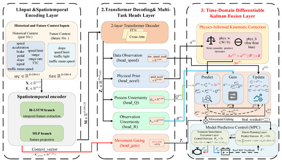
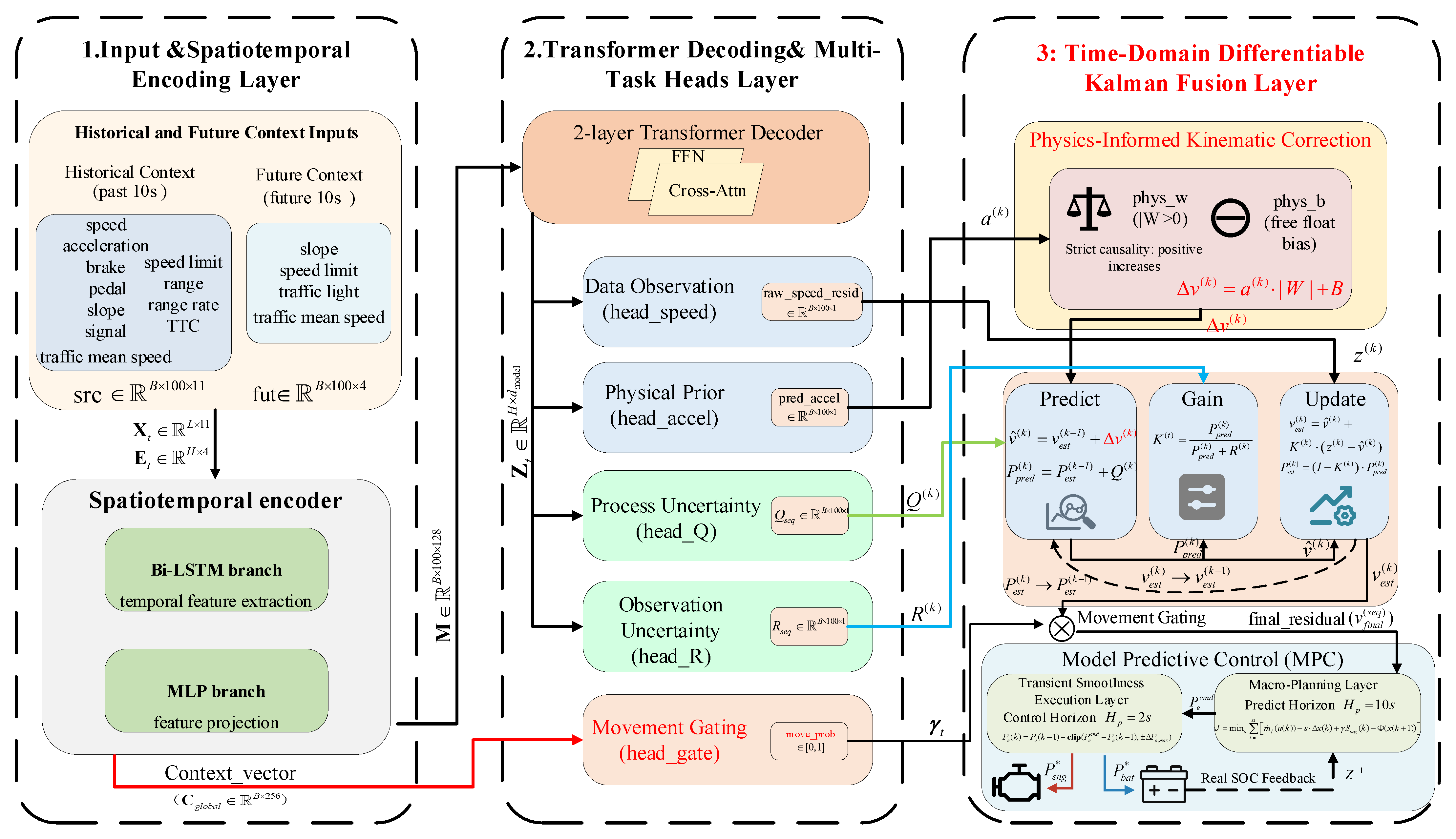
This paper focuses on the energy management system of HEVs. This section presents the proposed framework in a progressive manner, from the establishment of physical boundaries to receding horizon optimization. First, the vehicle’s longitudinal dynamics and multivariable physical constraints are constructed to establish the absolute physical boundaries of the system’s energy flow. Second, based on a high-fidelity traffic dataset, the long-horizon vehicle velocity prediction problem is formulated in the state space. On this foundation, the core architecture and physics-informed components of PI-STN are introduced in detail. Finally, the MPC energy allocation strategy, which utilizes the PI-STN prediction sequence as a feedforward reference, is expounded. The overall architecture of the proposed predictive energy management system is illustrated in Figure 1.

Figure 1. Energy management framework based on PI-STN for MPC.

2.1. HEV Powertrain Modeling and Kinematic Constraints

The energy management evaluation in this study is conducted using a control-oriented HEV whole-vehicle simulation model implemented in Python3.11. As described in Section 2.1, the longitudinal vehicle dynamics are first used to calculate the required vehicle power from the reconstructed speed and acceleration profiles. Then, the powertrain model incorporates the main energy-flow components required for EMS analysis, including the engine fuel-consumption map, motor power constraints, battery SOC dynamics, and MPC-based engine–battery power allocation. Therefore, the simulation platform forms a closed-loop vehicle-level energy management model for evaluating the influence of prediction quality on fuel economy, SOC regulation, and engine transient behavior. The model is control-oriented and focuses on energy management performance, rather than detailed chassis, thermal, or actuator-level dynamics.

2.1.1. Drivetrain System and Power Demand Modeling

For hybrid powertrain systems with complex mechanical inertia, MPC-based receding horizon optimization relies on accurate estimation of the vehicle power demand. Based on the principles of vehicle longitudinal dynamics [19], the total required power of the vehicle ${\mathit{P}}_{\mathit{req}}(\mathit{t})$ at any time step $\mathit{t}$ is determined jointly by road resistance and transient inertial force, which is mathematically expressed as follows:

$${\mathit{P}}_{\mathit{r}\mathit{e}\mathit{q}}(\mathit{t})={\displaystyle \frac{\mathit{v}(\mathit{t})}{{\mathit{\eta }}_{\mathit{T}}}}\left(\mathit{m}\mathit{g}\mathit{f}\mathbf{cos}\mathit{\theta }(\mathit{t})+{\displaystyle \frac{1}{2}}{\mathit{\rho }}_{\mathit{a}}{\mathit{C}}_{\mathit{d}}{\mathit{A}}_{\mathit{f}}\mathit{v}{(\mathit{t})}^2+\mathit{m}\mathit{g}\mathbf{sin}\mathit{\theta }(\mathit{t})+\mathit{\delta }\mathit{m}\cdot \mathit{a}(\mathit{t})\right)$$

(1)

where $\mathit{v}(\mathit{t})$ (m/s) and $\mathit{a}(\mathit{t})$ (m/s²) are the transient velocity and acceleration of the vehicle, respectively; $\mathit{\theta }(\mathit{t})$ is the road gradient; $\mathit{m}$ (kg) is the vehicle mass; $\mathit{f}$ is the rolling resistance coefficient; ${\mathit{\rho }}_{\mathit{a}}$ (kg/m³) is the air density; ${\mathit{C}}_{\mathit{d}}$ is the aerodynamic drag coefficient; ${\mathit{A}}_{\mathit{f}}$ (m²) is the frontal area; $\mathit{\delta }$ is the rotational mass conversion coefficient; and ${\mathit{\eta }}_{\mathit{T}}$ is the comprehensive efficiency of the transmission system.

As can be seen from the above equation, the vehicle’s power demand is not only a nonlinear function of velocity $\mathit{v}(\mathit{t})$, but also exhibits a positive correlation amplification effect with the first derivative of velocity, i.e., acceleration $\mathit{a}(\mathit{t})$. This implies that when high-frequency numerical disturbances exist in the predicted velocity sequence, these high-frequency disturbances are highly susceptible to being amplified by the transient inertial term ($\mathit{\delta }\mathit{m}\cdot \mathit{a}(\mathit{t})$) during the calculation of power demand. This error propagation phenomenon, triggered by calculus operators, is one of the important factors that can exacerbate high-frequency oscillations in the power commands of downstream controllers.

2.1.2. Multivariable Physical and Transient Boundary Constraints

When executing energy allocation, the system must first satisfy the mechanical energy conservation of the vehicle’s required power:

$${\mathit{P}}_{\mathit{r}\mathit{e}\mathit{q}}(\mathit{t})={\mathit{P}}_{\mathit{e}\mathit{n}\mathit{g}}(\mathit{t})+{\mathit{P}}_{\mathit{m}\mathit{o}\mathit{t}}(\mathit{t})$$

(2)

where ${\mathit{P}}_{\mathit{r}\mathit{e}\mathit{q}}(\mathit{t})$ is the required mechanical power of the vehicle at time step $\mathit{t}$ (kW); ${\mathit{P}}_{\mathit{e}\mathit{n}\mathit{g}}(\mathit{t})$ and ${\mathit{P}}_{\mathit{m}\mathit{o}\mathit{t}}(\mathit{t})$ are the output mechanical powers of the engine and the traction motor at that moment, respectively (kW).

Under the premise of meeting the required power of the vehicle, the system’s energy allocation is constrained by the mechanical and electrochemical boundaries of each executing component. For the engine and traction motor, their output mechanical power must comply with the external characteristic envelope determined by the current rotational speed $\mathit{\omega }(\mathit{t})$:

$$\left\{\begin{array}{l}{\mathit{P}}_{\mathit{e}\mathit{n}\mathit{g}\_\mathit{m}\mathit{i}\mathit{n}}(\mathit{\omega })\le {\mathit{P}}_{\mathit{e}\mathit{n}\mathit{g}}(\mathit{t})\le {\mathit{P}}_{\mathit{e}\mathit{n}\mathit{g}\_\mathit{m}\mathit{a}\mathit{x}}(\mathit{\omega })\hfill \\ {\mathit{P}}_{\mathit{m}\mathit{o}\mathit{t}\_\mathit{m}\mathit{i}\mathit{n}}(\mathit{\omega })\le {\mathit{P}}_{\mathit{m}\mathit{o}\mathit{t}}(\mathit{t})\le {\mathit{P}}_{\mathit{m}\mathit{o}\mathit{t}\_\mathit{m}\mathit{a}\mathit{x}}(\mathit{\omega })\hfill \end{array}\right.$$

(3)

where $\mathit{\omega }(\mathit{t})$ is the corresponding current mechanical rotational speed (rad/s); ${\mathit{P}}_{\mathit{e}\mathit{n}\mathit{g}\_\mathit{m}\mathit{i}\mathit{n}}(\mathit{\omega })$ and ${\mathit{P}}_{\mathit{e}\mathit{n}\mathit{g}\_\mathit{m}\mathit{a}\mathit{x}}(\mathit{\omega })$ are the minimum and maximum output powers physically allowable for the engine at that speed, respectively (kW); ${\mathit{P}}_{\mathit{m}\mathit{o}\mathit{t}\_\mathit{m}\mathit{i}\mathit{n}}(\mathit{\omega })$ and ${\mathit{P}}_{\mathit{m}\mathit{o}\mathit{t}\_\mathit{m}\mathit{a}\mathit{x}}(\mathit{\omega })$ are the maximum generating (negative power limit) and maximum driving (positive power limit) boundaries of the motor at the current speed, respectively (kW). To clarify the rotational-speed operating profile used in the component constraints, the speed-related operating condition in this study is generated from the reconstructed driving cycle described in Section 2.2.1. The engine speed is determined according to the fuel-consumption map, which maps the MPC-commanded engine power to the corresponding fuel-efficient speed–torque operating point.

Simultaneously, the actual power output of the motor is subject to the transient charge and discharge capability of the power battery. Its corresponding battery terminal electrical power ${\mathit{P}}_{\mathit{b}\mathit{a}\mathit{t}}(\mathit{t})$ must satisfy the safety threshold based on the current State of Charge ($\mathit{S}\mathit{O}\mathit{C}$):

$${\mathit{P}}_{\mathit{b}\mathit{a}\mathit{t}\_\mathit{m}\mathit{i}\mathit{n}}(\mathit{S}\mathit{O}\mathit{C})\le {\mathit{P}}_{\mathit{b}\mathit{a}\mathit{t}}(\mathit{t})\le {\mathit{P}}_{\mathit{b}\mathit{a}\mathit{t}\_\mathit{m}\mathit{a}\mathit{x}}(\mathit{S}\mathit{O}\mathit{C})$$

(4)

where ${\mathit{P}}_{\mathit{b}\mathit{a}\mathit{t}}(\mathit{t})$ is the actual electrical power throughput of the battery (kW); ${\mathit{P}}_{\mathit{b}\mathit{a}\mathit{t}\_\mathit{m}\mathit{i}\mathit{n}}(\mathit{S}\mathit{O}\mathit{C})$ and ${\mathit{P}}_{\mathit{b}\mathit{a}\mathit{t}\_\mathit{m}\mathit{a}\mathit{x}}(\mathit{S}\mathit{O}\mathit{C})$ are the maximum transient charging and discharging power limits of the battery determined by the current $\mathit{S}\mathit{O}\mathit{C}$ level, respectively (kW).

To characterize the trade-off between fuel economy and engine transient smoothness, the transient transition constraint of the engine is explicitly considered. Considering the inherent physical inertia of the mechanical structure, the power step change rate of the engine has a physical upper limit in actual control:

$$|{\mathit{P}}_{\mathit{e}\mathit{n}\mathit{g}}(\mathit{t})-{\mathit{P}}_{\mathit{e}\mathit{n}\mathit{g}}(\mathit{t}-1)|\le \Delta {\mathit{P}}_{\mathit{l}\mathit{i}\mathit{m}\mathit{i}\mathit{t}}$$

(5)

where ${\mathit{P}}_{\mathit{e}\mathit{n}\mathit{g}}(\mathit{t}-1)$ is the actual engine power in the previous control period; $\Delta {\mathit{P}}_{\mathit{l}\mathit{i}\mathit{m}\mathit{i}\mathit{t}}$ is the maximum power change step physically permitted within a unit control period (kW). When severe phase lag or high-frequency disturbances exist in the upstream prediction sequence, the downstream MPC may trigger this hard boundary more frequently, causing the actual operating point to deviate from the system’s OOL and operate in less efficient regions.

2.2. Data Acquisition and Predictive Problem Formulation

2.2.1. High-Fidelity Continuous Trajectory Reconstruction

To train and validate the proposed PI-STN model with high generalization capability, vehicle trajectory data with high temporal continuity and rich traffic context is required. Unlike traditional driving cycles that only contain basic vehicle kinematic states, predictive energy management strategies require future traffic priors. Therefore, this study utilizes the Waymo Open Dataset, which natively includes abundant V2X context information, such as traffic light states, road speed limits, and traffic flow velocities. In a future connected environment, this information can be acquired via V2X communication to serve as future traffic priors.

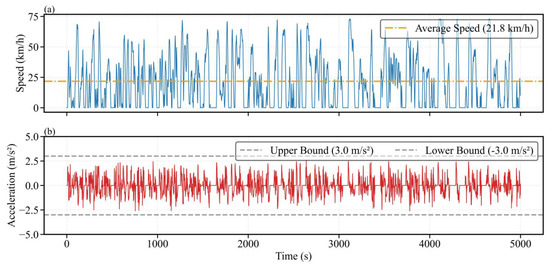
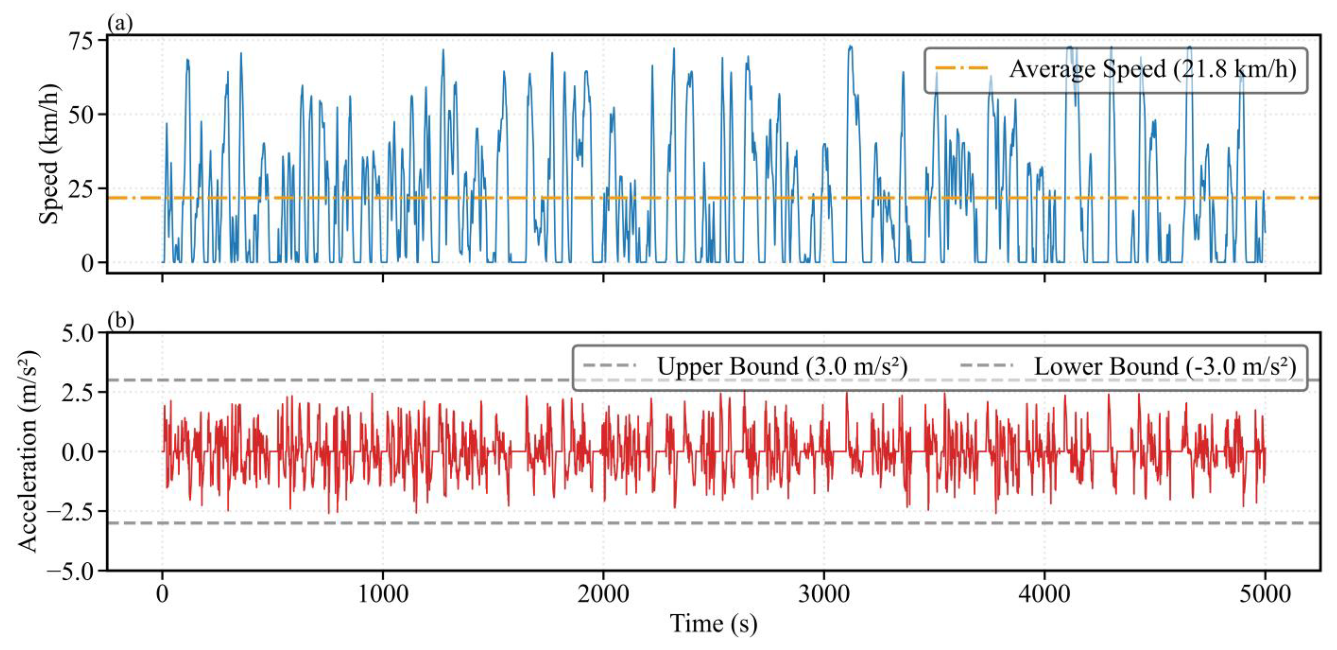
Given that the original Waymo data segments are typically short, a trajectory stitching method based on kinematic consistency constraints is employed to generate continuous trajectories suitable for HEV energy management strategy. During the stitching process, candidate segments are first screened through velocity continuity constraints, selecting the trajectory with the minimum velocity difference from the end of the previous segment. Subsequently, a cosine smoothing interpolation method is applied at the stitching boundaries to prevent acceleration mutations. To further eliminate high-frequency noise generated during stitching, a maximum acceleration physical truncation is enforced, and a Savitzky–Golay filter is utilized for smoothing. After these processes, a continuous driving trajectory totaling approximately 100,000 s is constructed. Its average velocity is 21.78 km/h, the maximum velocity is 77.07 km/h, the maximum acceleration is 2.86 m/s², the maximum braking deceleration is −3.14 m/s², and the sampling interval is 0.1 s. A typical trajectory segment from the dataset is shown in Figure 2. Figure 2a shows the representative speed trajectory of the reconstructed driving cycle, while Figure 2b presents the corresponding acceleration distribution together with the predefined operational bounds.

Figure 2. Typical kinematic profiles of the evaluated driving cycle. (a) Speed trajectory over the testing duration, indicating an average speed of 21.8 km/h; (b) Corresponding acceleration distribution with explicitly defined upper (3.0 m/s²) and lower (−3.0 m/s²) operational bounds.

2.2.2. State-Space Formulation of the Prediction Problem

In the predictive energy management strategy framework, vehicle velocity prediction is essentially a multivariable conditional sequence generation problem constrained by physical boundaries. At any given current time step $t$, the model input is decoupled into two heterogeneous tensors: a historical dynamic sequence and a future environmental prior sequence. First, the historical dynamic observation matrix ${\mathcal{X}}_t\in {ℝ}^{L\times 11}$ with a length of $L$ is defined as:

$${\mathcal{X}}_t={[x_{t-L+1},x_{t-L+2},\dots ,x_t]}^T$$

(6)

where the feature vector $x_i\in {ℝ}^{11}$ at a single time step encompasses 11 dimensions: ego-vehicle velocity, longitudinal acceleration, traffic signal state, traffic flow velocity, road gradient, speed limit, following distance $d_{r,i}$, relative velocity $v_{r,i}$, accelerator pedal opening, brake pedal state, and Time-To-Collision (TTC). To explicitly quantify the collision risk, TTC is strictly defined and capped at a physical upper limit of 20 s to avoid the numerical singularity that occurs when the relative velocity of the preceding vehicle approaches zero:

$$TT{C}_i=\min \left({\displaystyle \frac{d_{r,i}}{v_{r,i}+ϵ}},20\right)$$

(7)

where $ϵ$ is an infinitesimally small constant to prevent division by zero.

In parallel, the future environmental prior matrix ${\mathcal{E}}_t\in {ℝ}^{H\times 4}$ with a prediction horizon of $H$ is defined as:

$${\mathcal{E}}_t={[e_{t+1},e_{t+2},\dots ,e_{t+H}]}^T$$

(8)

where the feature vector $e_j\in {ℝ}^4$ contains 4 dimensions of traffic context features: traffic light signals, traffic flow velocity, road gradient, and road speed limits. Serving as a summary of future road conditions, these features guide the prediction model to respond to upcoming traffic variations in advance, thereby alleviating some limitations of traditional sequence prediction models [9,13].

2.2.3. Robustness Enhancement and Dataset Partition

To enhance the model’s robustness against transient sensor failures in real-world driving scenarios, a dynamic sequence masking enhancement strategy is introduced during the training phase. For samples in the training set, there is a 30% probability of randomly forcing 5 to 20 consecutive time steps in the historical velocity sequence to zero. This adversarial masking compels the model to learn deeper spatiotemporal dynamic dependencies rather than simple numerical translations. Finally, the first 80% of the dataset is allocated as the training set, and the remaining 20% serves as the testing set, so as to avoid data leakage between training and testing.

Based on the state-space definitions above, the velocity prediction task can be mathematically formalized as finding a physics-informed mapping function ${\mathcal{M}}_{\theta }(\cdot )$ (i.e., the PI-STN model) to infer the high-fidelity future velocity sequence ${\mathcal{Y}}_t\in {ℝ}^{H\times 1}$ given ${\mathcal{X}}_t$ and ${\mathcal{E}}_t$:

$${\mathcal{Y}}_t={\mathcal{M}}_{\theta }({\mathcal{X}}_t,{\mathcal{E}}_t)$$

(9)

$${\mathcal{Y}}_t={[{\widehat{v}}_{t+1},{\widehat{v}}_{t+2},\dots ,{\widehat{v}}_{t+H}]}^T$$

(10)

2.3. Physics-Informed Spatio-Temporal Network (PI-STN) Architecture

Under the previously defined state space, this section presents the proposed PI-STN framework. Rather than relying solely on numerical loss fitting, the framework is constructed as a unified prediction architecture that integrates physical causal constraints, DKF, and global zero-speed gating. Through this coordinated multi-component design, vehicle kinematic priors are embedded into the deep feature space of the network to improve both the physical consistency and the control-oriented quality of long-horizon velocity prediction [20].

2.3.1. Spatiotemporal Encoding and Future Alignment

For the historical dynamic observation matrix ${\mathcal{X}}_t\in {ℝ}^{L\times 11}$, considering that a pure Transformer encoder lacks a strict local temporal continuity inductive bias, while a unidirectional RNN struggles to capture global state dependencies, this study employs a two-layer Bi-LSTM network for spatiotemporal encoding [15,21]. The forward propagation chain of the Bi-LSTM highly conforms to the temporal evolution laws of vehicle physical inertia, while its backward tracing mechanism can fully integrate the contextual features before and after transient states [22].

After being encoded by the Bi-LSTM and subjected to a linear dimensionality reduction projection, ${\mathcal{X}}_t$ generates a deep and continuous comprehensive historical spatiotemporal memory matrix ${\mathcal{H}}_X\in {ℝ}^{L\times d_{model}}$. To extract the macroscopic motion intention within the historical window (e.g., acceleration to cruise or emergency braking trends), the final hidden state of the forward propagation ${\overrightarrow{h}}_L$ and the initial hidden state of the backward propagation ${\overleftarrow{h}}_1$ from the second layer are extracted and concatenated along the feature dimension to obtain a highly generalized global context vector $C_t$:

$$C_t=[{\overrightarrow{h}}_L\oplus {\overleftarrow{h}}_1]\in {ℝ}^{d_{model}}$$

(11)

where $\oplus$ denotes the feature concatenation operation; $C_t$ highly condenses the evolutionary trend of the historical trajectory and serves as a critical physical anchor for the subsequent computation of the macroscopic motion gating.

In parallel, for the future environmental prior matrix ${\mathcal{E}}_t\in {ℝ}^{H\times 4}$, its features exhibit significant differences in numerical scales and physical distributions compared to the dynamic sequence. Direct input is prone to causing cross-domain gradient imbalance. Therefore, a nonlinear projection operator ${\mathcal{F}}_{proj}$ with Layer Normalization is introduced to map it into a unified hidden dimension, yielding the aligned future prior embedding ${\mathcal{E}}_{aligned}\in {ℝ}^{H\times d_{model}}$.

2.3.2. Future Intent Decoding via Cross-Attention

When facing a long-horizon prediction task with, traditional autoregressive architectures tend to accumulate numerical errors due to step-by-step propagation, which may reduce prediction reliability over long horizons [10,23]. To address this limitation, PI-STN introduces a Transformer decoder based on multi-head cross-attention. This mechanism alters the step-by-step decoding paradigm and directly constructs a global mapping channel that spans the temporal dimension [20,24]. To adapt to the dynamic prediction task, a specific physical formulation is applied to the input tensors of the cross-attention mechanism. The Query matrix represents the model’s exploration of future states at each time step, determined jointly by environmental priors, macroscopic intentions, and temporal positional encoding:

$$Q={\mathcal{E}}_{aligned}+\mathrm{Repeat}(C_t)+PE$$

(12)

where $\mathrm{Repeat}(\cdot )$ denotes broadcasting and copying the context vector along the prediction horizon $H$; $PE$ is the positional encoding tensor based on sine and cosine functions.

The Key and Value matrices are directly derived from the historical spatiotemporal memory matrix, i.e., $K={\mathcal{H}}_X$ and $V={\mathcal{H}}_X$. Through the multi-head scaled dot-product attention mechanism, the decoder dynamically calculates the similarity weights between the future environmental priors and all historical transients, thereby computing a weighted aggregation of historical physical memories. After deep decoding and concatenation mapping by $N$ attention heads, the cross-domain fused deep representation matrix ${\mathcal{Z}}_t\in {ℝ}^{H\times d_{model}}$ is ultimately outputted. This matrix helps alleviate temporal dependency decay in long-horizon prediction and improves alignment with future prediction steps on the time axis.

2.3.3. Differentiable Kalman Filter (DKF)

To suppress the differential amplification effect triggered by pure data-driven models at the downstream control end, the PI-STN introduces a time-domain DKF layer behind the decoder [25]. This layer integrates the high-dimensional representation capability of deep networks with kinematic state-space equations.

First, through parallel linear perception heads, the predictive parameters for any future time step $t+k$ ($k\in [1,H]$) are dynamically decoded from the representation matrix ${\mathcal{Z}}_t$:

$$[z^{(k)},{\tilde{a}}^{(k)},q^{(k)},r^{(k)}]=W_{dec}\cdot {\mathcal{Z}}_t^{(k)}+b_{dec}$$

(13)

where $z^{(k)}$ is the pseudo-observation velocity residual inferred by the network; ${\tilde{a}}^{(k)}$ is the dimensionless prior acceleration feature; $q^{(k)}$ and $r^{(k)}$ are the process noise and observation noise covariances in logarithmic space, respectively; $W_{dec}$ and $b_{dec}$ are the weights and biases of the perception heads.

To map the dimensionless feature ${\tilde{a}}^{(k)}$ into a physical velocity increment $\Delta v^{(k)}$, and to reduce causal departure anomalies (e.g., the true state requires deceleration but the network outputs an acceleration trend), a decoupled physical calibration equation based on an absolute value constraint is introduced:

$$\Delta v^{(k)}=\left|W_{phys}\right|\cdot {\tilde{a}}^{(k)}+b_{phys}$$

(14)

where $W_{phys}$ and $b_{phys}$ are globally learnable physical calibration parameters independent of the network backbone. By applying the absolute value operator ($|\cdot |$) to the weight $W_{phys}$, the system establishes a physically consistent causal mapping: ensuring a strict monotonically increasing relationship between acceleration and velocity increments. The bias term $b_{phys}$ serves as a heterogeneous error absorber, adaptively compensating for environmental gravity components and measurement offsets and acquisition noise floors.

Upon obtaining $\Delta v^{(k)}$ that strictly follows physical causality, the system executes a continuous Kalman recursion within the prediction horizon. The state prediction step calculates the prior velocity ${\widehat{v}}_{pri}^{(k)}$ based on the optimal a posteriori estimate from the previous time step:

$${\widehat{v}}_{pri}^{(k)}={\widehat{v}}_{post}^{(k-1)}+\Delta v^{(k)}$$

(15)

Subsequently, in the state update step, the system calculates the dynamic Kalman gain $K_g^{(k)}$ to perform adaptive trust allocation between the kinematic prior estimate and the data-driven pseudo-observation:

$${\widehat{v}}_{post}^{(k)}={\widehat{v}}_{pri}^{(k)}+K_g^{(k)}\left({\widehat{v}}_{post}^{(k-1)}+z^{(k)}-{\widehat{v}}_{pri}^{(k)}\right)$$

(16)

After full-horizon deduction, the micro-level a posteriori prediction sequence ${\widehat{\mathcal{V}}}_t={[{\widehat{v}}_{post}^{(1)},\dots ,{\widehat{v}}_{post}^{(H)}]}^T$, which is phase-aligned and with reduced high-frequency non-physical fluctuations, is outputted.

2.3.4. Global Zero-Speed Gating

Under urban congestion or traffic light waiting conditions, due to sensor noise floors and network fitting inertia, pure data-driven prediction models may output small high-frequency numerical perturbations that approach but do not equal zero. This pseudo-motion can induce energy misjudgments by the MPC in control [26], triggering unnecessary engine starts and stops. To address this, the PI-STN establishes a cross-layer global zero-speed gating mechanism at the output end.

First, a cross-layer intent injection path is constructed. The global context anchor $C_t$ extracted in Section 2.3.1 is directly connected to the terminal gating operator ${\mathcal{F}}_{gate}$ to calculate the future macroscopic motion probability ${\gamma }_t$:

$${\gamma }_t=\sigma (W_{gate}\cdot C_t+b_{gate})$$

(17)

where $\sigma (\cdot )$ is the Sigmoid activation function; ${\gamma }_t\in (0,1)$ is essentially a macroscopic semantic discrimination of whether the vehicle will remain stationary within the future $H$ steps (approaching 0 indicates stopping and waiting, while approaching 1 indicates continuous motion).

Finally, an output-end hard gating fusion is executed. The micro-level optimal sequence ${\widehat{\mathcal{V}}}_t$ from the DKF layer and the macroscopic motion probability ${\gamma }_t$ are subjected to an element-wise physical mapping:

$${\mathcal{Y}}_t={\gamma }_t\odot {\widehat{\mathcal{V}}}_t$$

(18)

where $\odot$ represents the Hadamard product. When the global semantics determine that the vehicle is in an idling condition (${\gamma }_t\to 0$), the prediction sequence is constrained to the physical zero position. This dual-layer physical synergistic mechanism helps suppress zero-speed drift, and the generated high-fidelity sequence ${\mathcal{Y}}_t$ is directly dispatched to the MPC controller as a feedforward parameter.

2.4. Physics-Aware Multi-Task Loss Formulation

Traditional time-series prediction models mostly rely on a single MSE as the objective function. In the long-horizon prediction tasks for HEVs, merely constraining the absolute numerical values at each time step often causes the model to incline toward generating overly smoothed mean predictions. This phenomenon may induce noticeable kinematic phase lag under transient conditions such as hard acceleration or deceleration. To jointly improve numerical accuracy, physical consistency, and multi-task feature decoding, a physics-aware multi-task loss function is designed for end-to-end optimization of PI-STN [27]. The total loss function ${\mathcal{L}}_{\mathit{t}\mathit{o}\mathit{t}\mathit{a}\mathit{l}}$ is decoupled into a basic state regression loss and physical intent auxiliary constraint terms. Its overall mathematical formulation is defined as follows:

$${\mathcal{L}}_{\mathit{t}\mathit{o}\mathit{t}\mathit{a}\mathit{l}}={\mathcal{L}}_{\mathit{s}\mathit{p}\mathit{e}\mathit{e}\mathit{d}}+{\mathit{\lambda }}_{\mathit{d}\mathit{e}\mathit{r}\mathit{i}\mathit{v}}{\mathcal{L}}_{\mathit{d}\mathit{e}\mathit{r}\mathit{i}\mathit{v}}+{\mathit{\lambda }}_{\mathit{a}\mathit{c}\mathit{c}\mathit{e}\mathit{l}}{\mathcal{L}}_{\mathit{a}\mathit{c}\mathit{c}\mathit{e}\mathit{l}}+{\mathit{\lambda }}_{\mathit{g}\mathit{a}\mathit{t}\mathit{e}}{\mathcal{L}}_{\mathit{g}\mathit{a}\mathit{t}\mathit{e}}$$

(19)

where ${\mathcal{L}}_{\mathit{s}\mathit{p}\mathit{e}\mathit{e}\mathit{d}}$ is the velocity regression loss of the final output sequence; ${\mathcal{L}}_{\mathit{d}\mathit{e}\mathit{r}\mathit{i}\mathit{v}}$ is the first-order temporal derivative loss; ${\mathcal{L}}_{\mathit{a}\mathit{c}\mathit{c}\mathit{e}\mathit{l}}$ and ${\mathcal{L}}_{\mathit{g}\mathit{a}\mathit{t}\mathit{e}}$ are the prior acceleration loss and macroscopic motion gating loss from the intermediate multi-task decoding heads of the network, respectively; ${\mathit{\lambda }}_{\mathit{d}\mathit{e}\mathit{r}\mathit{i}\mathit{v}}$, ${\mathit{\lambda }}_{\mathit{a}\mathit{c}\mathit{c}\mathit{e}\mathit{l}}$ and ${\mathit{\lambda }}_{\mathit{g}\mathit{a}\mathit{t}\mathit{e}}$ are static hyperparameters used to balance the gradients across different optimization spaces (empirically set to 0.05, 0.5, and 0.5, respectively, considering the magnitude differences of each physical quantity). The detailed calculation equations for each branch loss function are as follows:

$$\left\{\begin{array}{l}{\mathcal{L}}_{\mathit{s}\mathit{p}\mathit{e}\mathit{e}\mathit{d}}={\displaystyle \frac{1}{\mathit{B}\cdot \mathit{H}}}{\displaystyle \sum _{\mathit{i}=1}^{\mathit{B}}{\displaystyle \sum _{\mathit{k}=1}^{\mathit{H}}\Vert {\mathit{v}}_{\mathit{f}\mathit{i}\mathit{n}\mathit{a}\mathit{l}}^{(\mathit{k})}-{\mathit{v}}_{\mathit{g}\mathit{t}}^{(\mathit{k})}{\Vert }_2^2}}\hfill \\ {\mathcal{L}}_{\mathit{d}\mathit{e}\mathit{r}\mathit{i}\mathit{v}}={\displaystyle \frac{1}{\mathit{B}\cdot \mathit{H}}}{\displaystyle \sum _{\mathit{i}=1}^{\mathit{B}}{\displaystyle \sum _{\mathit{k}=1}^{\mathit{H}}\Vert {\nabla }_{\mathit{k}}{\mathit{v}}_{\mathit{f}\mathit{i}\mathit{n}\mathit{a}\mathit{l}}^{(\mathit{k})}-{\nabla }_{\mathit{k}}{\mathit{v}}_{\mathit{g}\mathit{t}}^{(\mathit{k})}{\Vert }_1}}\hfill \\ {\mathcal{L}}_{\mathit{a}\mathit{c}\mathit{c}\mathit{e}\mathit{l}}={\displaystyle \frac{1}{\mathit{B}\cdot \mathit{H}}}{\displaystyle \sum _{\mathit{i}=1}^{\mathit{B}}{\displaystyle \sum _{\mathit{k}=1}^{\mathit{H}}\Vert {\mathit{a}}^{(\mathit{k})}-{\mathit{a}}_{\mathit{g}\mathit{t}}^{(\mathit{k})}{\Vert }_2^2}}\hfill \\ {\mathcal{L}}_{\mathit{g}\mathit{a}\mathit{t}\mathit{e}}=-{\displaystyle \frac{1}{\mathit{B}}}{\displaystyle \sum _{\mathit{i}=1}^{\mathit{B}}\left({\mathit{p}}_{\mathit{g}\mathit{t}}\mathit{log}({\mathit{p}}_{\mathit{m}\mathit{o}\mathit{v}\mathit{e}})+(1-{\mathit{p}}_{\mathit{g}\mathit{t}})\mathit{log}(1-{\mathit{p}}_{\mathit{m}\mathit{o}\mathit{v}\mathit{e}})\right)}\hfill \end{array}\right.$$

(20)

where $\mathit{B}$ is the training batch size; $\mathit{H}$ is the prediction horizon length; ${\mathit{v}}_{\mathit{f}\mathit{i}\mathit{n}\mathit{a}\mathit{l}}^{(\mathit{k})}$ and ${\mathit{v}}_{\mathit{g}\mathit{t}}^{(\mathit{k})}$ represent the final predicted velocity and the ground truth velocity corresponding to time step $\mathit{t}$, respectively; ${\mathit{a}}^{(\mathit{k})}$ and ${\mathit{a}}_{\mathit{g}\mathit{t}}^{(\mathit{k})}$ represent the network-decoded prior acceleration and the ground truth acceleration, respectively; ${\mathit{p}}_{\mathit{m}\mathit{o}\mathit{v}\mathit{e}}$ is the macroscopic motion probability output by the network; ${\mathit{p}}_{\mathit{g}\mathit{t}}\in \{0,1\}$ is the macroscopic motion label extracted from the real trajectory (set to 1 if a non-zero velocity exists within the future $\mathit{H}$ steps, and 0 otherwise). It is worth noting that when calculating the first-order temporal derivative loss ${\mathcal{L}}_{\mathit{d}\mathit{e}\mathit{r}\mathit{i}\mathit{v}}$, the temporal gradient operator ${\nabla }_{\mathit{k}}$ is introduced, and it is constrained by the ${\mathit{L}}_1$ norm instead of the ${\mathit{L}}_2$ norm to enhance the model’s sensitivity in capturing transient acceleration mutations.

Through the aforementioned joint training strategy, the PI-STN effectively guarantees the kinematic consistency of the predicted trajectories while improving the velocity prediction accuracy.

2.5. MPC-Based Predictive Energy Management Strategy

To fully unleash the potential of the high-fidelity future traffic priors provided by the PI-STN model, an MPC energy management strategy framework is constructed. MPC explicitly handles multi-component dynamic couplings and transient physical constraints within a receding optimization horizon. Combining it with a feedforward prediction sequence helps alleviate the limitations of traditional causal control strategies that rely mainly on current-state information.

2.5.1. Energy Mapping and Cost Function Formulation

First, the controller receives the high-fidelity predicted velocity sequence ${\mathcal{Y}}_{\mathit{t}}={[{\widehat{\mathit{v}}}^{(1)},\dots ,{\widehat{\mathit{v}}}^{(\mathit{H})}]}^{\mathit{T}}$ output by the PI-STN and the road gradient sequence ${\Theta }_{\mathit{t}}={[{\widehat{\mathit{\theta }}}^{(1)},\dots ,{\widehat{\mathit{\theta }}}^{(\mathit{H})}]}^{\mathit{T}}$ from the future environmental prior matrix. Based on the longitudinal dynamics equation established in Section 2.1.1 (Equation (1)), the MPC utilizes inverse calculation to accurately map them into the required mechanical power sequence of the vehicle ${\mathcal{P}}_{\mathit{r}\mathit{e}\mathit{q}}={[{\widehat{\mathit{P}}}_{\mathit{r}\mathit{e}\mathit{q}}^{(1)},\dots ,{\widehat{\mathit{P}}}_{\mathit{r}\mathit{e}\mathit{q}}^{(\mathit{H})}]}^{\mathit{T}}$ over the prediction horizon $\mathit{H}$. This sequence serves as the absolute energy conservation baseline for the MPC receding horizon optimization.

Based on this energy mapping, the core optimization objective of the MPC is to minimize fuel consumption and maintain the battery SOC balance while satisfying the vehicle’s power demand. This study defines the one-dimensional state variable as $\mathit{x}(\mathit{k})$ and the control variable as the engine output power $\mathit{u}(\mathit{k})$. The receding horizon objective function $\mathit{J}$ within the prediction window $[\mathit{t},\mathit{t}+\mathit{H}]$ is formulated as a composite incorporating equivalent fuel consumption, charge-sustaining penalties, and engine start-stop penalties [28]:

$$\mathit{J}={\mathbf{min}}_{\mathit{u}}{\displaystyle \sum _{\mathit{k}=1}^{\mathit{H}}\left[{\dot{\mathit{m}}}_{\mathit{f}}(\mathit{u}(\mathit{k}))-\mathit{s}\cdot \Delta \mathit{x}(\mathit{k})+\mathit{\gamma }{\mathit{S}}_{\mathit{e}\mathit{n}\mathit{g}}(\mathit{k})+\mathsf{\Phi }(\mathit{x}(\mathit{k}+1))\right]}$$

(21)

where $\mathit{s}$ is the adaptive equivalence factor; ${\dot{\mathit{m}}}_{\mathit{f}}(\cdot )$ is the instantaneous fuel consumption rate corresponding to the engine’s transient power; ${\mathit{S}}_{\mathit{e}\mathit{n}\mathit{g}}(\mathit{k})$ is the engine start indicator variable; and $\mathit{\gamma }$ is the start-stop penalty weight. The term $\mathsf{\Phi }(\mathit{x})$ is a quadratic soft-boundary penalty designed for the charge-sustaining mode, formulated as:

$$\mathsf{\Phi }(x)=\left\{\begin{array}{ll}{\lambda }_{low}{(x_{target}-x)}^2,\hfill & \mathrm{if} x<x_{target}\hfill \\ {\lambda }_{high}{(x-x_{upper})}^2,\hfill & \mathrm{if} x>x_{upper}\hfill \\ 0,\hfill & \mathrm{otherwise}\hfill \end{array}\right.$$

(22)

This soft-boundary mechanism allows the SOC to fluctuate elastically within a reasonable range, but once it touches the physical safety limits, a massive penalty threshold ${\mathit{\lambda }}_{\mathit{i}\mathit{n}\mathit{f}}$ is triggered.

2.5.2. Receding Horizon Optimization and Constraint Solving

At each control step $\mathit{t}$, the MPC converts the aforementioned cost function into a constrained nonlinear programming problem for online solving. To ensure the safety and lifespan of the components, the controller must strictly adhere to the following physical boundary constraints:

$$\mathbf{s}.\mathbf{t}. \left\{\begin{array}{l}\mathit{S}\mathit{O}{\mathit{C}}_{\mathit{m}\mathit{i}\mathit{n}}\le \mathit{x}(\mathit{k})\le \mathit{S}\mathit{O}{\mathit{C}}_{\mathit{m}\mathit{a}\mathit{x}}\hfill \\ {\mathit{P}}_{\mathit{e}\mathit{n}\mathit{g},\mathit{m}\mathit{i}\mathit{n}}(\mathit{\omega })\le \mathit{u}(\mathit{k})\le {\mathit{P}}_{\mathit{e}\mathit{n}\mathit{g},\mathit{m}\mathit{a}\mathit{x}}(\mathit{\omega })\hfill \\ {\mathit{P}}_{\mathit{m}\mathit{o}\mathit{t},\mathit{m}\mathit{i}\mathit{n}}(\mathit{\omega })\le {\mathit{P}}_{\mathit{r}\mathit{e}\mathit{q}}(\mathit{k})-\mathit{u}(\mathit{k})\le {\mathit{P}}_{\mathit{m}\mathit{o}\mathit{t},\mathit{m}\mathit{a}\mathit{x}}(\mathit{\omega })\hfill \end{array}\right.$$

(23)

where ${\mathit{P}}_{\mathit{e}\mathit{n}\mathit{g},\mathit{m}\mathit{i}\mathit{n}/\mathit{m}\mathit{a}\mathit{x}}$ and ${\mathit{P}}_{\mathit{m}\mathit{o}\mathit{t},\mathit{m}\mathit{i}\mathit{n}/\mathit{m}\mathit{a}\mathit{x}}$ are the physical power limits of the engine and motor, respectively, which vary dynamically with the current rotational speed $\mathit{\omega }$.

Meanwhile, to improve engine transient smoothness without increasing the dimensionality of the state space, this paper adopts a two-level decoupled architecture of macroscopic energy planning—low-level physical execution. When the macroscopic optimal command ${\mathit{u}}^{*}(\mathit{k})$ planned by the MPC is dispatched to the actuator, it must comply with the transient smoothness physical constraints brought about by the mechanical inertia of the engine rotor:

$${\mathit{u}}_{\mathit{r}\mathit{e}\mathit{a}\mathit{l}}(\mathit{k})=\mathbf{sat}\left({\mathit{u}}^{*}(\mathit{k}),{\mathit{u}}_{\mathit{r}\mathit{e}\mathit{a}\mathit{l}}(\mathit{k}-1)\pm \Delta {\mathit{P}}_{\mathit{s}\mathit{t}\mathit{e}\mathit{p}}\right)$$

(24)

where $\Delta {\mathit{P}}_{\mathit{s}\mathit{t}\mathit{e}\mathit{p}}$ is the maximum physically permissible power change step within a unit control period, and $\mathbf{sat}(\cdot )$ is the boundary truncation function.

Benefiting from the suppression of high-frequency non-physical fluctuations and the correction of zero-speed drift by the front-end PI-STN, the demand power sequence fed forward to the controller becomes smoother and more consistent with kinematic causality. This helps the MPC optimizer plan the control trajectory with fewer activations of the hard truncation limits. As a result, transient engine power fluctuations are reduced, and the operating point can be maintained closer to the OOL, thereby improving the coordination between predictive planning and physical execution.

3. Results

3.1. Experiment Setup and Evaluation Metrics

To systematically evaluate the trajectory prediction capability of the proposed PI-STN and its macroscopic impact on downstream hybrid energy management strategy, rigorous validation was conducted based on a real-world autonomous driving high-frequency trajectory dataset. All training and simulations were executed on a high-performance workstation equipped with an Intel Core i7 processor and an NVIDIA RTX 5070Ti GPU. The historical observation window and future prediction horizon of the PI-STN are both set to 10 s (corresponding to $\mathit{H}=100$ steps, sampling period $\Delta \mathit{t}=0.1 \mathrm{s}$). Despite the broad attention paid to purely data-driven methods, they face challenges in physical boundary constraints and temporal consistency due to their black-box nature [29,30,31]. Therefore, we selected representative baseline models for comparison [32]: (1) LSTM; (2) BiLSTM-Transformer; and (3) Transformer-KF. The selected baselines are intended to cover several representative categories of long-horizon velocity prediction methods used in predictive energy management. LSTM represents a classical recurrent neural network baseline, BiLSTM-Transformer represents an attention-enhanced sequence prediction model, and Transformer-KF represents a hybrid data-driven filtering framework. In addition, MPC-Perfect is introduced in the downstream energy management evaluation as an ideal-preview reference, while DP is reported only as an offline benchmark. Therefore, the comparison focuses on evaluating whether the proposed PI-STN can provide more control-oriented prediction information than representative data-driven and hybrid prediction models under the same EMS framework.

To evaluate the computational efficiency and real-time feasibility of the proposed prediction module, a runtime analysis was conducted using the same workstation as that used for training and simulation. Since model training is performed offline, onboard implementation mainly depends on the inference time required for one receding-horizon prediction. Therefore, the inference time was measured with batch size 1 after warm-up runs and averaged over repeated forward passes. The prediction horizon is 10 s, corresponding to 100 future steps with a sampling interval of 0.1 s. Detailed computational statistics are provided in Appendix B.

The evaluation framework comprises four dimensions. First, $\mathit{R}\mathit{M}\mathit{S}\mathit{E}$ and $\mathit{M}\mathit{A}\mathit{E}$ evaluate the overall deviation:

$$\mathit{R}\mathit{M}\mathit{S}\mathit{E}=\sqrt{{\displaystyle \frac{1}{\mathit{H}}}{\displaystyle \sum _{\mathit{k}=1}^{\mathit{H}}{\left({\widehat{\mathit{v}}}^{(\mathit{k})}-{\mathit{v}}_{\mathit{g}\mathit{t}}^{(\mathit{k})}\right)}^2}}$$

(25)

$$\mathit{M}\mathit{A}\mathit{E}={\displaystyle \frac{1}{\mathit{H}}}{\displaystyle \sum _{\mathit{k}=1}^{\mathit{H}}\left|{\widehat{\mathit{v}}}^{(\mathit{k})}-{\mathit{v}}_{\mathit{g}\mathit{t}}^{(\mathit{k})}\right|}$$

(26)

where $\mathit{H}$ is the total number of time steps in the prediction horizon; ${\widehat{\mathit{v}}}^{(\mathit{k})}$ and ${\mathit{v}}_{\mathit{g}\mathit{t}}^{(\mathit{k})}$ represent the predicted velocity and the ground truth velocity at the $\mathit{k}$-th future time step, respectively.

Since downstream controllers are highly sensitive to high-frequency transients, Acceleration $\mathit{R}\mathit{M}\mathit{S}\mathit{E}$ (Acc-RMSE) is introduced to measure dynamic consistency:

$$\mathit{Acc}\text{-}\mathit{RMSE}=\sqrt{{\displaystyle \frac{1}{\mathit{H}-1}}{\displaystyle \sum _{\mathit{k}=1}^{\mathit{H}-1}{\left(\nabla {\widehat{\mathit{v}}}^{(\mathit{k})}-\nabla {\mathit{v}}_{\mathit{g}\mathit{t}}^{(\mathit{k})}\right)}^2}}$$

(27)

where $\nabla {\widehat{\mathit{v}}}^{(\mathit{k})}$ and $\nabla {\mathit{v}}_{\mathit{g}\mathit{t}}^{(\mathit{k})}$ denote the predicted acceleration and the ground truth acceleration, respectively.

Finally, Dynamic Time Warping (DTW) is employed to assess the overall manifold deformation of the sequence:

$$\mathbf{DTW}(\widehat{\mathit{V}},{\mathit{V}}_{\mathit{g}\mathit{t}})={\mathbf{min}}_{\mathcal{W}}{\displaystyle \sum _{\mathit{i}=1}^{\mathit{K}}\mathit{d}}({\mathit{w}}_{\mathit{i}})$$

(28)

where $\mathcal{W}$ represents the optimal alignment warping path and $\mathit{d}({\mathit{w}}_{\mathit{i}})$ is the Euclidean distance between the aligned data points at the $\mathit{i}$-th step of the path.

3.2. Microscopic Prediction Performance

Unlike conventional studies that focus mainly on point-to-point prediction errors, this section evaluates not only numerical fitting accuracy but also the physical causality, temporal stability, and robustness of the predicted trajectories under stationary scenarios.

3.2.1. Overall Prediction Accuracy Analysis

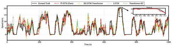
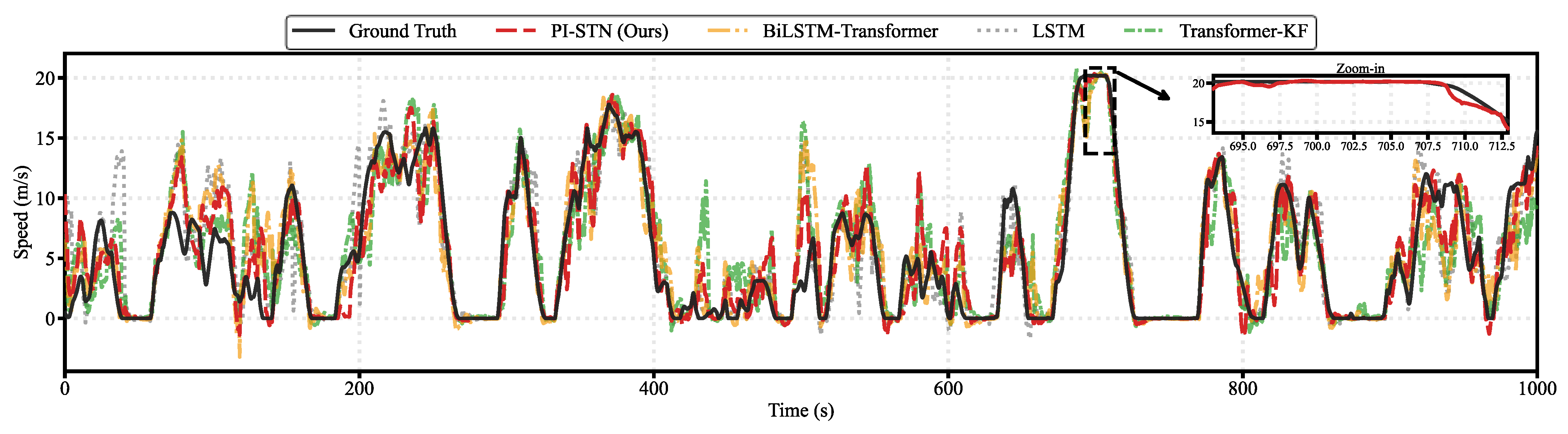
Figure 3 illustrates a macroscopic 1000 s velocity prediction trajectory. This extensive segment encompasses complex characteristics of real-world urban traffic flows, including frequent traffic-light start-stops, rapid accelerations/decelerations, and high-speed cruising. Qualitatively, when facing intense transient velocity switches, pure data-driven baseline models (such as LSTM and BiLSTM-Transformer) commonly exhibit noticeable phase lags and local high-frequency oscillations. By comparison, the prediction trajectory of PI-STN (red line) is smoother and remains closely aligned with the ground truth across major peaks and troughs. This suggests that the DKF module can attenuate spurious pseudo-observation perturbations during long-horizon extrapolation and help preserve the physically consistent evolution of vehicle motion under complex dynamic variations.

Figure 3. Comparison of velocity prediction trajectories in a typical driving segment.

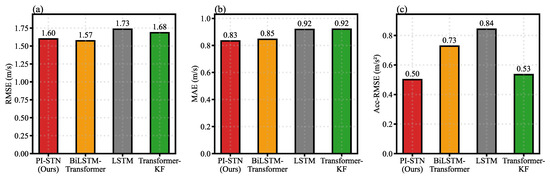
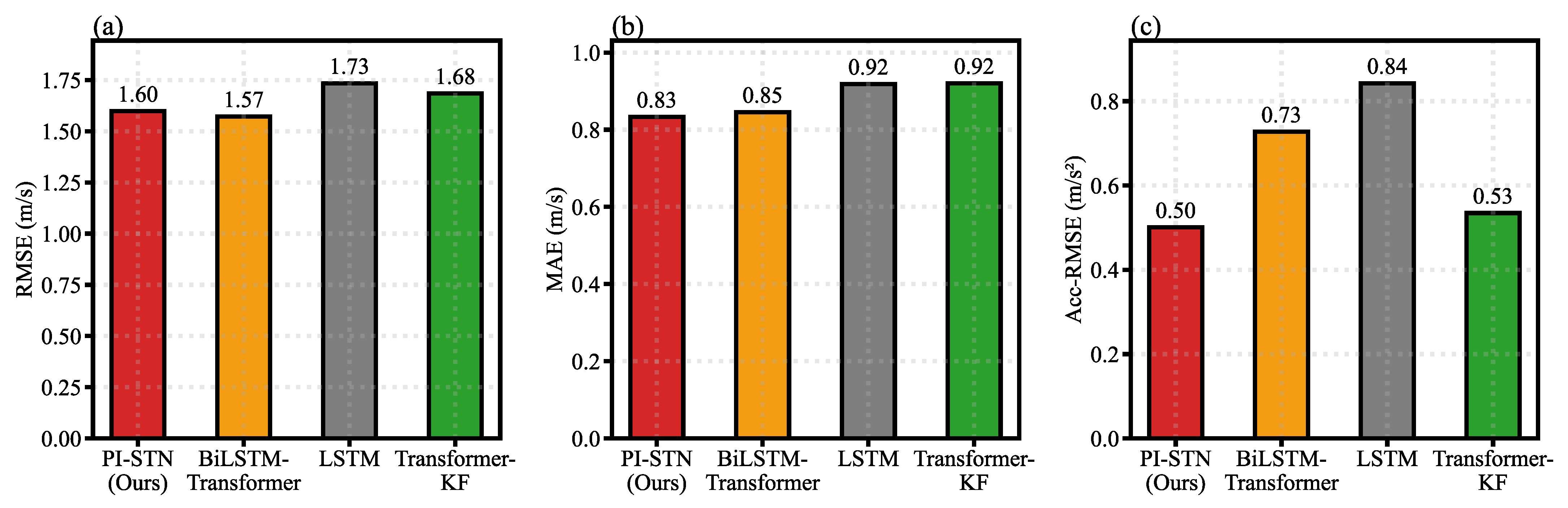
Figure 4 further provides quantitative evaluation bar charts for all models across the entire test set. In the velocity $\mathit{R}\mathit{M}\mathit{S}\mathit{E}$ comparison shown in Figure 4a, the pure data-driven BiLSTM-Transformer achieves an extremely low value of 1.57 m/s by leveraging its large-scale parameters for Euclidean space fitting. PI-STN (1.60 m/s) performs highly competitively, maintaining a rigorous baseline prediction standard. However, as shown in Figure 4b, PI-STN achieves the lowest overall $\mathit{M}\mathit{A}\mathit{E}$ of 0.83 m/s among the evaluated models. This result indicates that PI-STN can better suppress persistent systematic bias errors.

Figure 4. Quantitative comparison of microscopic evaluation metrics for different prediction models across the entire test set. (a) Comparison of velocity $\mathit{R}\mathit{M}\mathit{S}\mathit{E}$ for each model over the full prediction horizon; (b) Comparison of velocity $\mathit{M}\mathit{A}\mathit{E}$ for each model over the full prediction horizon; (c) Comparison of Acc-RMSE for each model in tracking transient dynamic characteristics.

More crucially, for the downstream hybrid energy management system, sheer absolute velocity error is insufficient to reflect the control-oriented quality of the predicted sequence. As illustrated in Figure 4c, PI-STN achieves the best Acc-RMSE among the evaluated models, which is a key metric for measuring the kinematic fidelity of the sequence. Its error is 0.50 m/s², lower than that of Transformer-KF (0.53 m/s²) and substantially lower than that of BiLSTM-Transformer (0.73 m/s²). These results indicate that the physical causal loss and the DKF architecture improve the model’s ability to capture first-order kinematic derivatives. By reducing non-physical jitters in the prediction sequence, the proposed method provides a more suitable input for downstream MPC and supports improvements in both fuel economy and powertrain operational smoothness.

Furthermore, to quantitatively evaluate the sequence-level trajectory fidelity and physical dynamic characteristics, the DTW distance is introduced in this paper. As shown in Table 1, in terms of the DTW metric—which measures the overall trajectory fidelity—PI-STN achieves the lowest value of 54.5072. Concurrently, the baseline model Transformer-KF exhibits the maximum comprehensive sequence deformation error (with a DTW as high as 61.2457). This further supports the effectiveness of integrating physical causal constraints into the spatio-temporal prediction architecture for reducing high-frequency distortions in pure data-driven models.

Table 1. Performance comparison of trajectory prediction models on the test dataset.

Model	RMSE (m/s)	MAE (m/s)	Acc-RMSE (m/s2)	DTW
LSTM	1.7345	0.9183	0.8426	59.5269
BiLSTM-Transformer	1.5715	0.8454	0.7274	55.4733
Transformer-KF	1.6845	0.9204	0.5347	61.2457
PI-STN (Ours)	1.5978	0.8330	0.5005	54.5072

3.2.2. Physical Causality and Temporal Stability

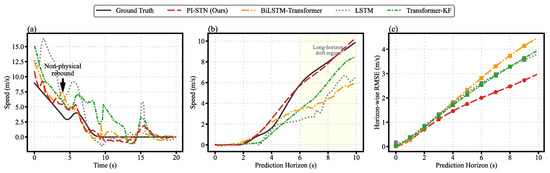
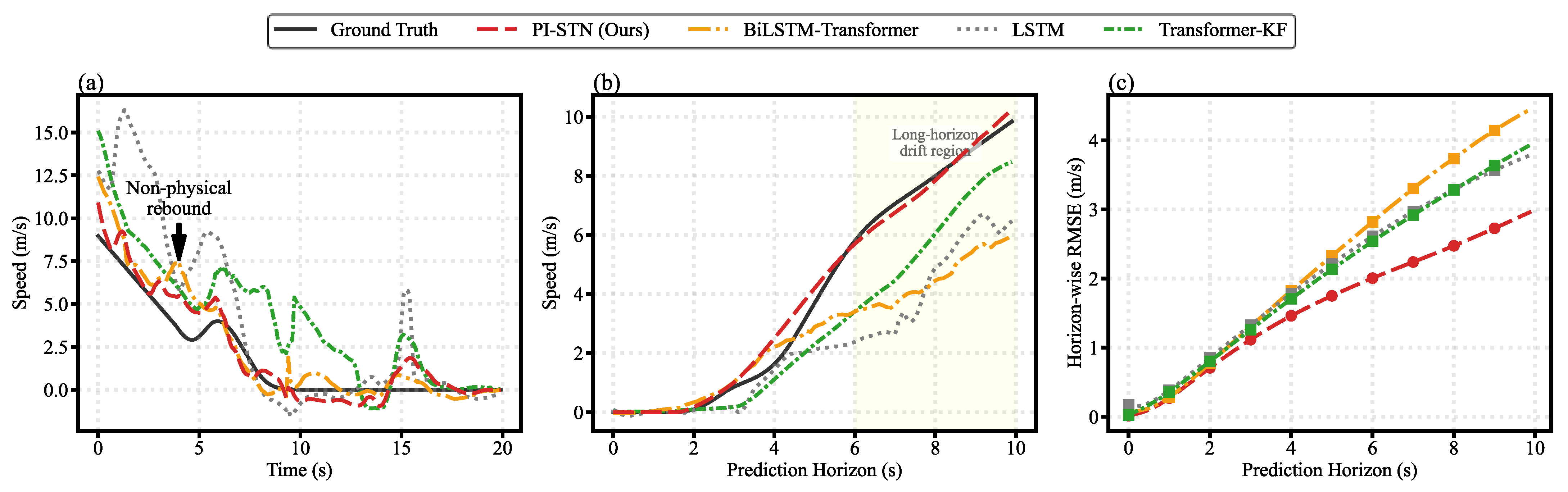
Long-horizon prediction should consider not only numerical fitting accuracy but also consistency with the vehicle’s underlying kinematic causality and the suppression of error accumulation in the temporal dimension. Figure 5 comprehensively illustrates the performance of various models in terms of physical causality and temporal stability. Figure 5a extracts a typical hard-braking scenario. It can be observed that while the actual vehicle speed continuously decreases, baseline models such as BiLSTM-Transformer exhibit severe non-physical velocity rebounds and overshoots. In contrast, the amplitude of velocity rebounds and overshoots in PI-STN is significantly reduced. To quantitatively evaluate the physical consistency of the prediction results from different models, this paper introduces the Physical Violation Rate (${\mathit{R}}_{\mathit{p}\mathit{v}}$) as an evaluation metric. This metric is used to measure the proportion of the model’s prediction results that violate fundamental kinematic causality, and its definition is:

$${\mathit{R}}_{\mathit{p}\mathit{v}}={\displaystyle \frac{{\mathit{N}}_{\mathit{v}\mathit{i}\mathit{o}\mathit{l}\mathit{a}\mathit{t}\mathit{i}\mathit{o}\mathit{n}}}{{\mathit{N}}_{\mathit{t}\mathit{o}\mathit{t}\mathit{a}\mathit{l}}}}\times 100\%$$

(29)

where ${\mathit{N}}_{\mathit{v}\mathit{i}\mathit{o}\mathit{l}\mathit{a}\mathit{t}\mathit{i}\mathit{o}\mathit{n}}$ represents the total number of time steps exhibiting physical causality violations within the prediction sequence, and ${\mathit{N}}_{\mathit{t}\mathit{o}\mathit{t}\mathit{a}\mathit{l}}$ is the total number of evaluated time steps. Specifically, a physical violation event is recorded when the actual vehicle exhibits a clear physical intention to accelerate or decelerate, yet the model predicts an opposing motion trend. The criteria for this determination encompass the following two scenarios:

Figure 5. Validation of physical causality and temporal stability for different prediction models. (a) Velocity prediction trajectories in a typical braking scenario, illustrating the causality violation phenomenon; (b) Temporal drift characteristics within a single 10 s prediction window; (c) Error accumulation over the prediction horizon represented by the horizon-wise $\mathit{R}\mathit{M}\mathit{S}\mathit{E}$.

1.

Braking violation: The actual vehicle is in a distinct deceleration state (true acceleration ${\mathit{a}}_{\mathit{g}\mathit{t}}<-\mathit{ϵ}$), but the model exhibits irrational acceleration (predicted acceleration ${\mathit{a}}_{\mathit{p}\mathit{r}\mathit{e}\mathit{d}}>{\mathit{ϵ}}^{\prime }$);

2.

Acceleration violation: The actual vehicle is in a distinct acceleration state (true acceleration ${\mathit{a}}_{\mathit{g}\mathit{t}}>\mathit{ϵ}$), but the model exhibits abnormal deceleration (predicted acceleration ${\mathit{a}}_{\mathit{p}\mathit{r}\mathit{e}\mathit{d}}<-{\mathit{ϵ}}^{\prime }$).

A lower value of this metric indicates that the model’s prediction results conform more strictly to fundamental dynamic laws. The data in Table 2 further demonstrate that, relying on its embedded physical causal constraints, PI-STN substantially curtails the global ${\mathit{R}}_{\mathit{p}\mathit{v}}$ to an overall lowest of 5.26%. By contrast, pure data-driven models lacking hard physical guidance (such as BiLSTM-Transformer and Transformer-KF) yield high physical violation rates of 7.27% and 6.25%, respectively; the classical LSTM method performs the worst, reaching up to 9.81%. Specifically, PI-STN achieves a remarkable 46.38% improvement in physical consistency compared to LSTM, and a significant 15.84% enhancement over the runner-up, Transformer-KF. These results support the effectiveness of integrating physical causality into the network architecture for reducing non-physical distortions in pure data-driven models. Figure 5b further illustrates the temporal drift behavior of different models within a single prediction window, whereas Figure 5c presents the horizon-wise RMSE evolution, revealing the error accumulation characteristics over the prediction horizon.

Table 2. Quantitative comparison of physical violation rates among different models.

Model	LSTM	BiLSTM-Transformer	Transformer-KF	PI-STN (Ours)
${\mathit{R}}_{\mathit{p}\mathit{v}}$	9.81%	7.27%	6.25%	5.26%

3.2.3. Dynamic Robustness Under Stationary Scenarios

In real-world urban traffic flows, vehicles experience extensive zero-speed phases when waiting at traffic lights or queuing in congestion. For pure data-driven time-series prediction models, such scenarios remain challenging. Owing to bias accumulation in network activations and unavoidable observation disturbances, the model output may still exhibit low-amplitude velocity drift even when the true vehicle speed remains zero, thereby producing pseudo-motion. In practical hybrid energy management systems, such misjudgments can easily mislead downstream controllers into erroneously determining that the vehicle is about to start up, thereby triggering unnecessary high-frequency engine start-stops and power allocations.

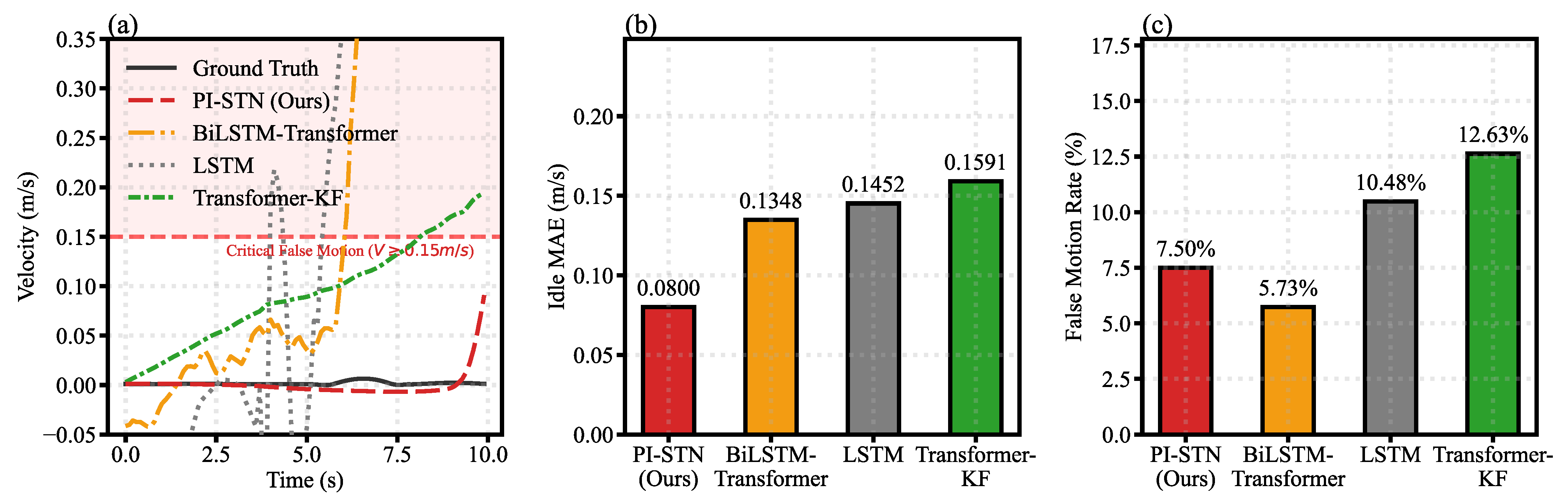
In actual Vehicle Control Units, a specific velocity deadband is typically established to filter out minor measurement noise. The control system only determines that the vehicle has started moving when the predicted speed breaches a specific threshold and persists for a certain duration. To this end, this paper formulates two types of zero-speed stability metrics: First, the set of idle time steps for the actual vehicle is defined as ${\mathcal{T}}_{\mathit{i}\mathit{d}\mathit{l}\mathit{e}}=\{\mathit{t}\mid {\mathit{v}}_{\mathit{t}\mathit{r}\mathit{u}\mathit{e}}(\mathit{t})<0.05\}$, representing all sampling instants where the true vehicle speed is within the sensor noise floor (0.05 m/s), with its total number of frames denoted as ${\mathit{N}}_{\mathit{i}\mathit{d}\mathit{l}\mathit{e}}$. The first metric is the Idle Mean Absolute Error (Idle MAE). Compared to the $\mathit{R}\mathit{M}\mathit{S}\mathit{E}$, which is highly sensitive to extreme outliers, $\mathit{M}\mathit{A}\mathit{E}$ provides a more authentic measurement of the model’s global noise floor level in the zero-speed region. The calculation formula is as follows:

$$\mathrm{Idle} \mathrm{MAE}={\displaystyle \frac{1}{N_{idle}}}{\displaystyle \sum _{t\in {\mathcal{T}}_{idle}}\left|v_{pred}(t)-v_{true}(t)\right|}$$

(30)

The second metric is the Continuous Critical False Motion Rate (${\mathit{R}}_{\mathit{f}\mathit{m}}^{\mathit{c}}$). This indicator aims to capture fatal prediction violations where the predicted velocity breaches the start-up static friction deadband (0.15 m/s) and continuously persists for a duration exceeding the actuator’s physical delay (0.3 s, corresponding to 3 time steps). This accurately reflects the substantive interference that the false-motion disturbances induced by prediction may impose on downstream control. The calculation formula is as follows:

$${\mathit{R}}_{\mathit{f}\mathit{m}}^{\mathit{c}}={\displaystyle \frac{1}{{\mathit{N}}_{\mathit{i}\mathit{d}\mathit{l}\mathit{e}}}}{\displaystyle \sum _{\mathit{t}\in {\mathcal{T}}_{\mathit{i}\mathit{d}\mathit{l}\mathit{e}}}{\mathbb{I}}_{\mathit{c}}}(\mathit{t})\times 100\%$$

(31)

where ${\mathbb{I}}_{\mathit{c}}(\mathit{t})=1$ if and only if ${\mathit{v}}_{\mathit{p}\mathit{r}\mathit{e}\mathit{d}}(\mathit{t})>0.15$ and the length of the continuous interval of this violation state is ≥3 frames; otherwise, ${\mathbb{I}}_{\mathit{c}}(\mathit{t})=0$.

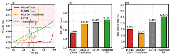
As illustrated in Figure 6a, within the zero-speed region, the prediction curve of PI-STN tightly adheres to the ground truth, achieving the lowest overall Idle MAE of 0.0800 m/s. In contrast, both LSTM (0.1452 m/s) and Transformer-KF (0.1591 m/s) exhibit significant divergence, while BiLSTM-Transformer (0.1348 m/s) even experiences local numerical instability during long-horizon extrapolation. Regarding the ${\mathit{R}}_{\mathit{f}\mathit{m}}^{\mathit{c}}$ metric, the violation rate of PI-STN is maintained at 7.50%. Although BiLSTM-Transformer achieves the nominally lowest value of 5.73%, its overall noise floor and numerical oscillation characteristics suggest limited robustness under idle conditions. This result may be related to local prediction behavior that does not continuously exceed the threshold, rather than to consistently stable zero-speed prediction performance. As shown in Figure 6b, PI-STN achieves the lowest Idle MAE among the evaluated models, indicating a lower global noise floor during idle periods. Figure 6c further compares the false-motion rates of different models and shows that PI-STN maintains a favorable balance between noise suppression and robustness under zero-speed conditions. In summary, through the combined effect of the global zero-speed gating mechanism and the DKF, PI-STN maintains a relatively low physical noise floor while suppressing continuous false activations, thereby providing a smoother and more reliable input for the HEV control system.

Figure 6. Evaluation of prediction stability and false motion suppression under idle conditions. (a) Velocity prediction trajectories during a ground-truth idle phase, illustrating the critical false motion phenomenon; (b) MAE of velocity predictions strictly within idle periods; (c) Statistical comparison of false motion rates across different prediction models.

3.3. Predictive Energy Management Strategy Performance

To evaluate the effectiveness of the proposed PI-STN prediction framework in downstream control, this section constructs an MPC-based Predictive Energy Management Strategy using the predicted velocity sequences. The controller employs a multi-objective cost function to minimize the battery SOC tracking error, reduce the engine’s Equivalent Fuel Consumption (EFC), and suppress engine transient power fluctuations. To provide an ideal-preview reference, an MPC-Perfect model with complete future vehicle speed preview capability is introduced.

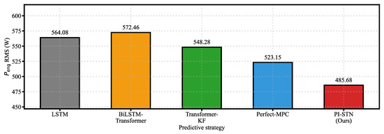
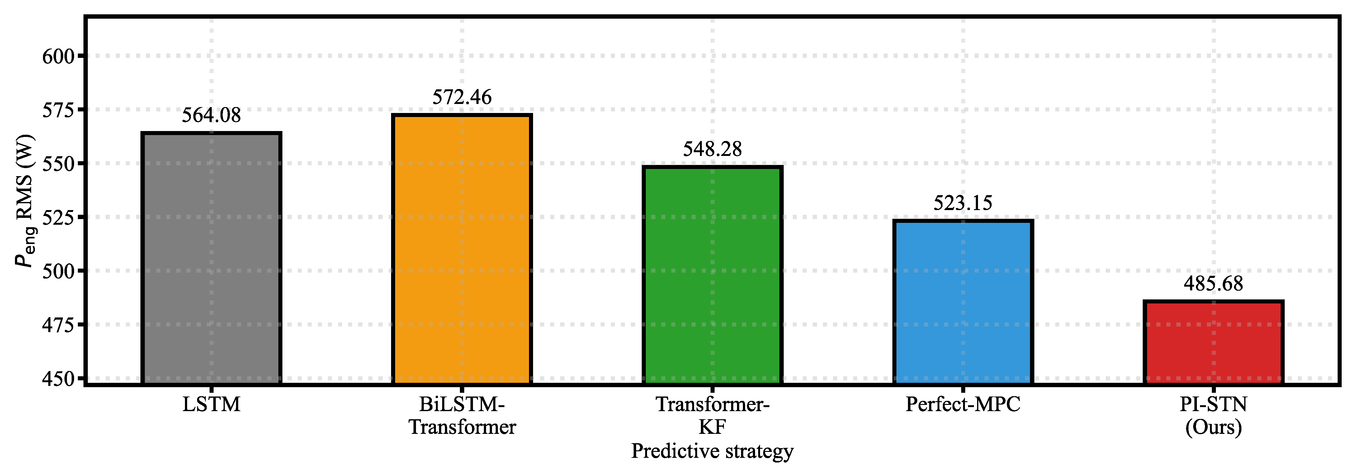
Table 3 summarizes the global quantitative results of different strategies over the entire test set under the nominal charge-sustaining setting. Among the online predictive methods, PI-STN achieves the lowest EFC of 323.74 g, compared with 324.08 g for LSTM, 331.46 g for BiLSTM-Transformer, and 334.16 g for Transformer-KF. In addition, PI-STN also yields the lowest engine power fluctuation, with a P_eng RMS of 485.68 W, which is 15.1% lower than that of the worst-performing BiLSTM-Transformer (572.46 W) and 14.0% lower than that of LSTM (564.08 W). Compared with MPC-Perfect, PI-STN still exhibits a lower EFC (323.74 g vs. 327.08 g) and a lower P_eng RMS (485.68 W vs. 523.15 W) under the evaluated conditions, suggesting that the smoother and more physically consistent predictive reference can be beneficial for online optimization. However, since slight differences remain in terminal SOC among the online strategies, the EFC results should be interpreted together with the final SOC values rather than as a fully isolated metric. In particular, DP is reported only as an offline reference benchmark, because its final SOC drops to 57.98%, which deviates substantially from the charge-sustaining target and is therefore not directly comparable with the online predictive strategies in terms of EFC.

Table 3. Performance comparison of different predictive energy management strategies.

Model	EFC (g)	P_eng RMS (W)	Final SOC (%)
LSTM	324.08	564.08	61.87%
BiLSTM-Transformer	331.46	572.46	61.47%
Transformer-KF	334.16	548.28	61.09%
PI-STN (Ours)	323.74	485.68	60.53%
MPC-Perfect	327.08	523.15	61.09%
DP	239.53	N/A	57.98%

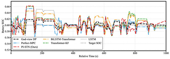
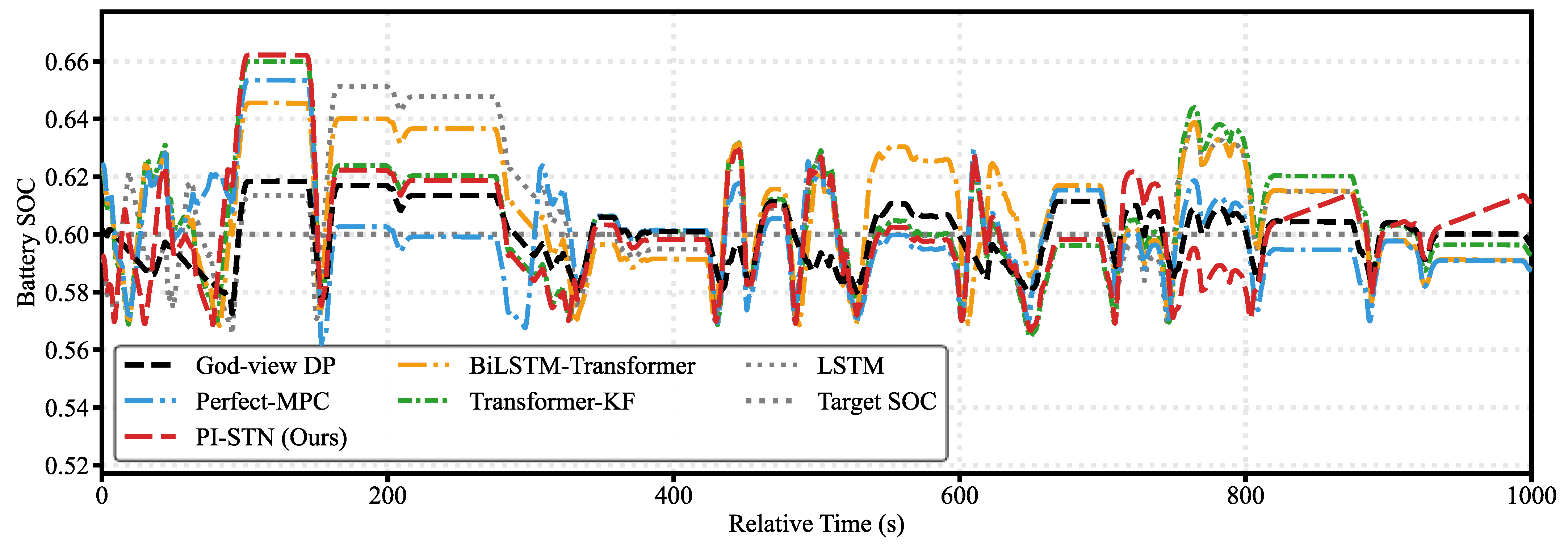
To intuitively illustrate the time-domain evolution characteristics of the aforementioned global quantitative metrics, Figure 7 extracts a typical SOC trajectory segment spanning 1000 s. It can be observed that under long-horizon continuous dynamic conditions, all baseline models manage to constrain the SOC near the target value of 0.60, indicating the basic robustness of the MPC framework. However, a closer examination of the curve morphology reveals that the SOC trajectory driven by PI-STN facilitates a smoother electrical energy throughput when encountering severe velocity fluctuations. It helps mitigate the charge–discharge oscillations induced by high-frequency distortions in the predicted velocities of pure data-driven models, thereby supporting smoother operation of downstream actuators.

Figure 7. Battery SOC trajectories of different predictive energy management strategies under the charge-sustaining mode.

To provide a clearer quantitative comparison of engine transient smoothness, Figure 8 presents the engine power fluctuation of different predictive energy management strategies, measured by P_eng RMS. A lower P_eng RMS indicates that the engine power command varies less sharply during transient operation, corresponding to smoother powertrain behavior. As shown in Figure 8, the proposed PI-STN achieves the lowest P_eng RMS of 485.68 W among all evaluated online predictive methods. Compared with LSTM and BiLSTM-Transformer, whose P_eng RMS values are 564.08 W and 572.46 W, respectively, PI-STN reduces engine power fluctuation by approximately 14.0% and 15.1%. Transformer-KF also improves transient smoothness to some extent, but its P_eng RMS remains higher than that of PI-STN. This result indicates that merely introducing a filtering mechanism is insufficient; the physical consistency and phase alignment of the predicted velocity sequence are also important for suppressing unnecessary engine power corrections. In addition, PI-STN exhibits a lower P_eng RMS than MPC-Perfect under the evaluated conditions, suggesting that a smoother control-oriented prediction sequence can be more beneficial for online power allocation than directly tracking all high-frequency components in the future velocity trajectory.

Figure 8. Comparison of engine power fluctuation among different predictive energy management strategies.

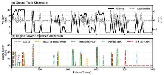
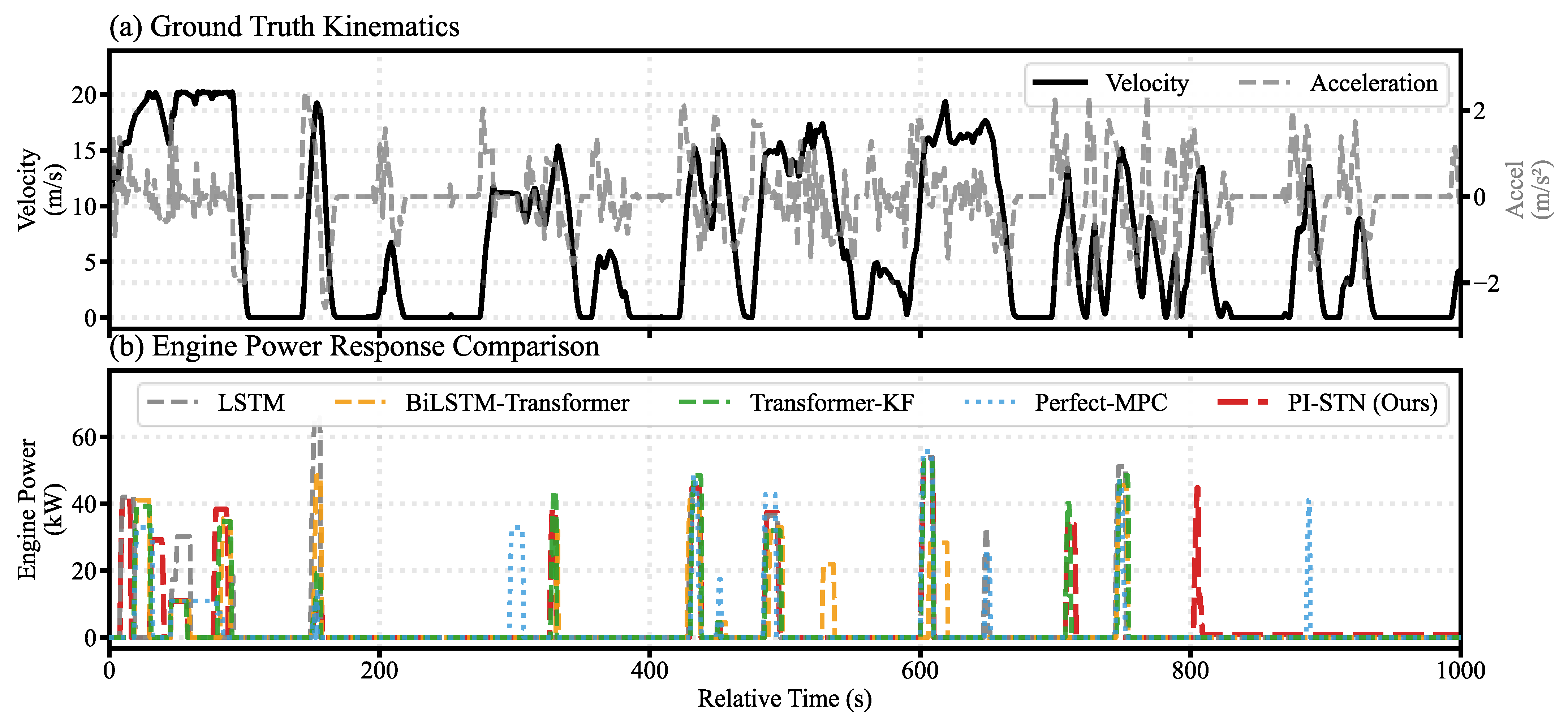
While Figure 8 provides a global statistical view of engine transient smoothness, Figure 9 further illustrates the time-domain response characteristics under a representative fluctuating driving segment. To further analyze how PI-STN improves the balance between fuel economy and powertrain smoothness, Figure 9 presents the dynamic characteristics of a typical 1000 s transient fluctuating condition. As shown in Figure 9a, real-world urban traffic flows contain extensive microscopic acceleration and deceleration switches, which manifest as the high-frequency oscillations of the gray acceleration line. Faced with such highly dynamic conditions, Figure 9b intuitively reflects the limitations of pure data-driven models lacking physical priors: owing to the difficulty in maintaining kinematic smoothness over the temporal horizon, models such as LSTM and BiLSTM-Transformer are prone to generating non-physical high-frequency velocity distortions within the prediction window. When tracking these high-frequency perturbations, the downstream MPC controller tends to trigger unnecessary power overshoots, exhibited as frequent engine start-stops and transient power pulses (as indicated by the dense dashed spikes in Figure 9b). Meanwhile, as previously mentioned, the MPC-Perfect model also incurs a certain degree of passive power oscillation due to its direct response to the high-frequency components inherent in real-world speed trajectories.

Figure 9. Comparison of engine transient response behaviors driven by different prediction models within the MPC framework. (a) Ground truth kinematics including velocity and acceleration profiles of the driving cycle; (b) Engine power response trajectories, demonstrating the impact of prediction quality on transient power fluctuations and control delays.

By contrast, the proposed PI-STN exhibits more robust dynamic regulation characteristics. Benefiting from the dynamic Kalman filtering of time-varying process noise by the DKF module, PI-STN can effectively filter out spurious high-frequency perturbations and extract the macroscopic physical trends of the vehicle’s kinetic transitions. Such a smooth prediction sequence with a high degree of physical consistency enables the MPC to circumvent the interference of short-term pseudo-features and conduct a more reasonable global power allocation. As shown by the red line in Figure 9b, the engine driven by PI-STN effectively reduces invalid transient interventions, operating smoothly only within intervals of sustained high-load demand. This helps explain why PI-STN can reduce both fuel consumption and power fluctuation under the evaluated operating conditions.

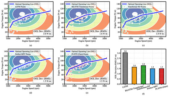
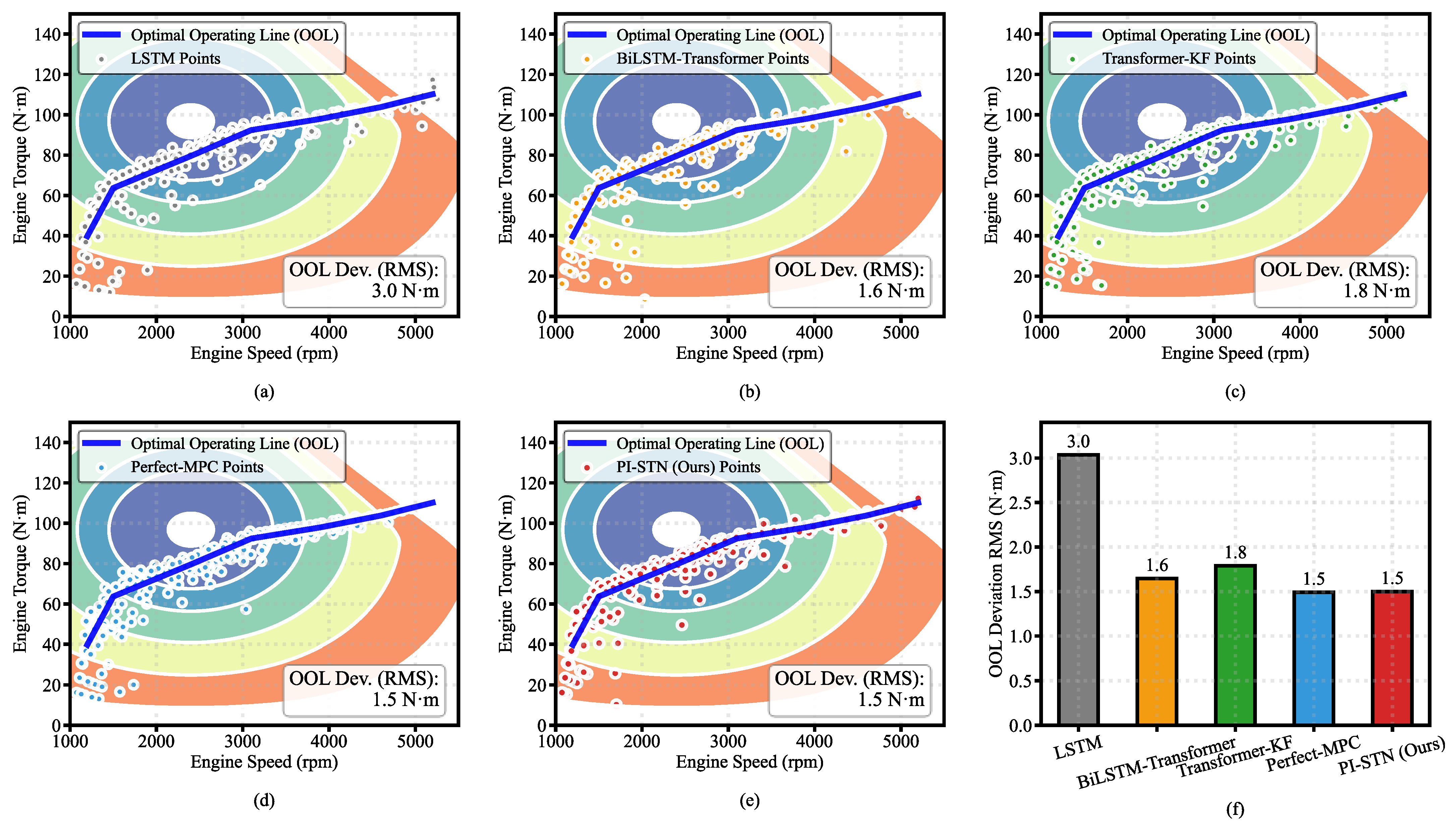
Furthermore, Figure 10 illustrates the scatter distribution of engine operating points on the Brake Specific Fuel Consumption (BSFC) map driven by various strategies. As shown in Figure 10a–c, under the guidance of traditional baseline models, the engine operating points predominantly exhibit a dispersed and phase-lagging state due to frequent jumps in high-frequency transient power. In contrast, as shown in Figure 10e, compared to the relatively scattered operating point distribution of the baseline methods, the results of PI-STN are highly concentrated near the high-efficiency region and exhibit a much smaller deviation from the OOL. This indicates that suppressing severe transient power fluctuations can help maintain engine operation within the high-efficiency region, thereby improving overall system performance while preserving fuel economy.

Figure 10. Evaluation of engine operating efficiency and dynamic deviation from the OOL. (a–e) Distribution of engine operating points on the Brake Specific Fuel Consumption (BSFC) map for LSTM, BiLSTM-Transformer, Transformer-KF, MPC-Perfect, and the proposed PI-STN, respectively; (f) Quantitative comparison of the Root Mean Square (RMS) deviation from the OOL across all evaluated methods. In the BSFC maps, the background contour colors indicate fuel-consumption levels, with blue/green regions representing lower BSFC and higher-efficiency operating areas, and yellow/orange regions representing higher BSFC and lower-efficiency operating areas. The blue curve denotes the optimal operating line (OOL), and the colored scatter points represent the engine operating points generated by each strategy.

The quantitative comparison bar chart in Figure 10f intuitively corroborates the aforementioned observations. Statistical results demonstrate that PI-STN substantially curtails the engine’s deviation from the OOL Deviation RMS from 3.0 N·m (for LSTM) to 1.5 N·m. This reduction reaches the same level as the ideal feedforward model, MPC-Perfect (1.5 N·m). These results suggest that maintaining the physical smoothness of the prediction sequence can help the underlying mechanical actuators operate closer to the optimal efficiency region.

Synthesizing the above analyses, it is evident that under strict Charge-Sustaining constraints, the role of a prediction model is reflected not only in macroscopic accuracy metrics but also, more substantially, in its impact on the quality of control decisions. By providing predictive information characterized by low latency and reduced non-physical fluctuations, PI-STN empowers the MPC to conduct forward-looking optimization more effectively. Consequently, it contributes to concurrent improvements in fuel economy and mechanical smoothness without introducing additional heuristic terms under the evaluated framework.

4. Discussion and Conclusions

Under strict charge-sustaining constraints, the differences in EFC among various methods are generally marginal, whereas their engine transient behaviors exhibit more noticeable divergence. This phenomenon indicates that the energy demand, dictated by external resistance under given driving conditions, establishes a physical lower bound for fuel consumption, causing the fuel economy of different strategies to converge. In contrast, the impact of prediction quality on control performance is primarily reflected in transient regulation.

The experimental results show that traditional models such as LSTM are prone to inducing control delays during rapid load changes due to phase lag in their predictions, which may lead to severe fluctuations in engine power. By improving temporal consistency, the proposed PI-STN provides more reliable look-ahead information for MPC. This allows the control strategy to rely more on active planning rather than passive correction, thereby reducing transient engine power fluctuations.

Mechanistically, the improvement in powertrain operational smoothness helps reduce the engine’s deviation from the optimal operating line. Under drastic power changes, phase-lagged speed prediction may force the engine into regions with higher specific fuel consumption, whereas smoother regulation helps maintain engine operation near the high-efficiency region. Therefore, the results of this study indicate that smoothness and economy are not necessarily mutually exclusive, and that a certain degree of coordinated improvement can be achieved through high-quality predictions.

From a broader perspective, this paper further illustrates that within the MPC framework, the value of a prediction model lies not only in numerical accuracy but also in its impact on control behavior, such as phase characteristics and dynamic consistency. This provides useful insights for the co-design of prediction models and control strategies in predictive energy management.

Several limitations of the present study should also be noted. First, although the driving trajectories and traffic-context inputs used in this study are reconstructed from real-world driving data, the downstream energy management validation is still conducted in a simulation environment. The adopted platform is a control-oriented HEV simulation model designed to evaluate the influence of prediction quality on fuel economy, SOC regulation, and engine transient behavior. Therefore, some real-vehicle effects, such as actuator delays, detailed thermal dynamics, sensor noise, communication latency, and hardware implementation constraints, are not fully represented in the current validation. These assumptions may influence the quantitative performance when the proposed method is deployed on an actual vehicle.

Second, the current framework does not explicitly provide calibrated probabilistic prediction intervals. The adaptive process and observation noise terms in the DKF module are mainly used for recursive filtering and phase alignment, rather than for full uncertainty quantification. In addition, the future traffic priors used by PI-STN are assumed to be reliable in the present study, whereas practical V2X inputs may be affected by communication latency, packet loss, sensor noise, and map-matching errors. Future work will further extend the proposed framework toward probabilistic velocity prediction and uncertainty-aware MPC under imperfect V2X information.

Third, the present study focuses on the system-level effectiveness of the integrated PI-STN framework in predictive energy management. Although the global zero-speed gating mechanism, physical causal penalty, and DKF module are designed to address complementary aspects of prediction consistency, namely zero-speed pseudo-motion, physical causality violation, and temporal phase misalignment, a dedicated component-wise ablation study is not included in the current manuscript. Such an ablation analysis would be valuable for quantitatively isolating the contribution of each module. In addition, comparisons with more classical physics-based predictors and recently proposed hybrid prediction models will be further expanded to more comprehensively position the proposed framework.

In future work, the proposed method will be further evaluated using Hardware-in-the-Loop (HIL) and real-vehicle platforms. Meanwhile, uncertainty-aware prediction, robust MPC under imperfect environmental priors, and component-wise ablation analysis will be investigated to further improve the practical applicability and interpretability of the proposed predictive energy management strategy.

References

- Zhang, Y.; Fan, P.; Lu, H.; Song, G. Fuel consumption of hybrid electric vehicles under real-world road and temperature conditions. Transp. Res. Part D Transp. Environ. 2025, 142, 104691. [Google Scholar] [CrossRef] [Scilit]
- Zhu, Y.; Li, X.; Liu, Q.; Li, S.; Xu, Y. Review article: A comprehensive review of energy management strategies for hybrid electric vehicles. Mech. Sci. 2022, 13, 147–188. [Google Scholar] [CrossRef] [Scilit]
- Azim Mohseni, N.; Bayati, N.; Ebel, T. Energy management strategies of hybrid electric vehicles: A comparative review. IET Smart Grid 2024, 7, 191–220. [Google Scholar] [CrossRef] [Scilit]
- Lü, X.; Li, S.; He, X.; Xie, C.; He, S.; Xu, Y.; Fang, J.; Zhang, M.; Yang, X. Hybrid electric vehicles: A review of energy management strategies based on model predictive control. J. Energy Storage 2022, 56, 106112. [Google Scholar] [CrossRef] [Scilit]
- Saifuddin, M.R.; Naayagi, R.T.; Tong, W.P.Q. Design and control of a DC collection system for modular-based direct electromechanical drive turbines in high voltage direct current transmission. Electronics 2020, 9, 493. [Google Scholar] [CrossRef] [Scilit]
- Poh, W.Q.T.; Naayagi, R.T. Modelling and integration of a piezoelectric cantilever beam with quasi-Z-source inverter for self-powered dynamic system application. In Proceedings of the 2020 IEEE Power & Energy Society General Meeting (PESGM), Montreal, QC, Canada, 2–6 August 2020; IEEE: Piscataway, NJ, USA, 2020; pp. 1–5. [Google Scholar]
- He, H.; Wang, Y.; Han, R.; Han, M.; Bai, Y.; Liu, Q. An improved MPC-based energy management strategy for hybrid vehicles using V2V and V2I communications. Energy 2021, 225, 120273. [Google Scholar]
- Yang, H.; Hu, Y.; Gong, X.; Cao, R.; Guo, L.; Chen, H. Energy management strategy for fuel cell hybrid electric vehicles considering the inaccuracy of predicted vehicle speed. IEEE Trans. Transp. Electrif. 2024, 10, 8246–8262. [Google Scholar] [CrossRef] [Scilit]
- East, S.; Cannon, M. Scenario model predictive control for data-based energy management in plug-in hybrid electric vehicles. IEEE Trans. Control Syst. Technol. 2022, 30, 2522–2533. [Google Scholar]
- Hou, S.; Chen, H.; Yin, H.; Zhao, J.; Xu, F.; Gao, J. Energy Management Based on Mixed-Integer Nonlinear Model Predictive Control for Hybrid Electric Vehicles. IEEE Trans. Intell. Transp. Syst. 2024, 25, 17432–17451. [Google Scholar] [CrossRef] [Scilit]
- Amini, M.R.; Hu, Q.; Wiese, A.; Kolmanovsky, I.; Buckland Seeds, J.; Sun, J. A data-driven spatio-temporal speed prediction framework for energy management of connected vehicles. IEEE Trans. Intell. Transp. Syst. 2023, 24, 291–303. [Google Scholar] [CrossRef] [Scilit]
- Ma, M.; Hu, J.; Xiao, R. Energy management strategy with model prediction for fuel cell hybrid trucks considering vehicle mass and road slope. Energy Convers. Manag. 2025, 333, 119791. [Google Scholar] [CrossRef] [Scilit]
- Kong, Y.; Xu, N.; Liu, Q.; Sui, Y.; Jia, Y. Variable horizon-based predictive energy management strategy for plug-in hybrid electric vehicles and determination of a suitable predictive horizon. Energy 2024, 294, 130809. [Google Scholar] [CrossRef] [Scilit]
- Lefèvre, S.; Sun, C.; Bajcsy, R.; Moura, S. Comparison of parametric and non-parametric approaches for vehicle speed prediction. In Proceedings of the 2014 American Control Conference, Portland, OR, USA, 4–6 June 2014; IEEE: Piscataway, NJ, USA, 2014; pp. 3494–3499. [Google Scholar]
- Li, T.; Cui, W.; Cui, N. Real-time multiobjective EMS for fuel cell vehicle considering energy source health awareness under unknown real-world conditions. IEEE Trans. Transp. Electrif. 2025, 11, 8936–8947. [Google Scholar] [CrossRef] [Scilit]
- Shen, H.; Wang, Z.; Zhou, X.; Lamantia, M.; Yang, K.; Chen, P.; Wang, J. Electric vehicle velocity and energy consumption predictions using Transformer and Markov-chain Monte Carlo. IEEE Trans. Transp. Electrif. 2022, 8, 3836–3847. [Google Scholar] [CrossRef] [Scilit]
- Wu, J.; Huang, Z.; Lv, C. Transformer-based traffic-aware predictive energy management of a fuel cell electric vehicle. IEEE Trans. Veh. Technol. 2024, 73, 4659–4670. [Google Scholar] [CrossRef] [Scilit]
- Li, Z.; Sun, H.; Xiao, D.; Xie, H. Hybrid Kalman recurrent neural network for vehicle trajectory prediction. IEEE Trans. Instrum. Meas. 2024, 73, 2519814. [Google Scholar] [CrossRef] [Scilit]
- Buggaveeti, S.; Batra, M.; McPhee, J.; Azad, N. Longitudinal vehicle dynamics modeling and parameter estimation for plug-in hybrid electric vehicle. SAE Int. J. Veh. Dyn. Stab. NVH 2017, 1, 289–297. [Google Scholar] [CrossRef] [Scilit]
- Geng, M.; Li, J.; Xia, Y.; Chen, X. A physics-informed Transformer model for vehicle trajectory prediction on highways. Transp. Res. Part C Emerg. Technol. 2023, 154, 104272. [Google Scholar] [CrossRef] [Scilit]
- Lu, D.; Hu, D.; Wang, J.; Wei, W.; Zhang, X. A data-driven vehicle speed prediction transfer learning method with improved adaptability across working conditions for intelligent fuel cell vehicle. IEEE Trans. Intell. Transp. Syst. 2025, 26, 10881–10891. [Google Scholar] [CrossRef] [Scilit]
- Feng, Z.; Zhang, J.; Jiang, H.; Yao, X.; Qian, Y.; Zhang, H. Energy consumption prediction strategy for electric vehicle based on LSTM-transformer framework. Energy 2024, 302, 131780. [Google Scholar] [CrossRef] [Scilit]
- Pulvirenti, L.; Rolando, L.; Millo, F. Energy management system optimization based on an LSTM deep learning model using vehicle speed prediction. Transp. Eng. 2023, 11, 100160. [Google Scholar] [CrossRef] [Scilit]
- Karniadakis, G.E.; Kevrekidis, I.G.; Lu, L.; Perdikaris, P. Physics-informed machine learning. Nat. Rev. Phys. 2021, 3, 422–440. [Google Scholar] [CrossRef] [Scilit]
- Chen, C.; Lu, C.X.; Wang, B.; Trigoni, N.; Markham, A. DynaNet: Neural Kalman dynamical model for motion estimation and prediction. IEEE Trans. Neural Netw. Learn. Syst. 2021, 32, 5479–5491. [Google Scholar] [CrossRef] [Scilit] [PubMed]
- Tang, X.; Hou, Y.; Qin, Y. Economical thermal energy management for hybrid electric vehicles based on multiple agents deep reinforcement learning. IEEE Trans. Transp. Electrif. 2026, 12, 3307–3318. [Google Scholar] [CrossRef] [Scilit]
- Raissi, M.; Perdikaris, P.; Karniadakis, G.E. Physics-informed neural networks: A deep learning framework for solving forward and inverse problems involving nonlinear partial differential equations. J. Comput. Phys. 2019, 378, 686–707. [Google Scholar] [CrossRef] [Scilit]
- Pisu, P.; Rizzoni, G. A comparative study of supervisory control strategies for hybrid electric vehicles. IEEE Trans. Control Syst. Technol. 2007, 15, 506–518. [Google Scholar] [CrossRef] [Scilit]
- Lian, R.; Peng, J.; Wu, Y.; Tan, H.; Zhang, H. Rule-interposing deep reinforcement learning based energy management strategy for power-split hybrid electric vehicle. Energy 2020, 197, 117297. [Google Scholar] [CrossRef] [Scilit]
- Shi, D.; Xu, H.; Wang, S.; Hu, J.; Chen, L.; Yin, C. Deep reinforcement learning based adaptive energy management for plug-in hybrid electric vehicle with double deep Q-network. Energy 2024, 305, 132402. [Google Scholar] [CrossRef] [Scilit]
- Chaudhary, R.; Sharma, N.K.; Kala, R.; Singh, S.N. Deep reinforcement learning-based speed predictor for distributionally robust eco-driving. IEEE Access 2025, 13, 13904–13918. [Google Scholar] [CrossRef] [Scilit]
- Zhang, L.; Liu, W.; Qi, B. Energy optimization of multi-mode coupling drive plug-in hybrid electric vehicles based on speed prediction. Energy 2020, 206, 118126. [Google Scholar]
Disclaimer/Publisher’s Note: The statements, opinions and data contained in all publications are solely those of the individual author(s) and contributor(s) and not of MDPI and/or the editor(s). MDPI and/or the editor(s) disclaim responsibility for any injury to people or property resulting from any ideas, methods, instructions or products referred to in the content. |
© 2026 by the authors. Licensee MDPI, Basel, Switzerland. This article is an open access article distributed under the terms and conditions of the Creative Commons Attribution (CC BY) license.