Operating Analysis and Driving Cycle Construction of Electric Passenger Vehicles Based on Real-World Operational Data

Abstract

Constructing the driving cycle of pure electric passenger vehicles (PEPVs) can provide a comprehensive understanding of the operational characteristics, thereby offering fundamental support for the continuous improvement of their performance. This study utilized the actual operational data of PEPVs to fully analyze and construct reliable drive cycles, aiming to mitigate deviations between standard cycles and real-world conditions and provide support for vehicle energy management and range assessment. First, the data were preprocessed, divided into short operational segments, and characterized by selecting typical feature values that sufficiently represent these segments. Second, principal component analysis (PCA) was employed to reduce the dimensionality of the features of each short segment, followed by clustering analysis using the k-means++ algorithm. Finally, the driving cycles were constructed based on the information from the short, clustered segments. Compared with the original data, the average relative error of the constructed driving cycles is 3.35%, indicating that the constructed driving cycles can effectively reflect the current operational characteristics of the PEPVs.

1. Introduction

Globally, accurately assessing vehicle energy consumption and emissions under real-world road conditions has become a critical challenge in the low-carbon transformation of the automotive industry. Although major markets worldwide have established standardized chassis dynamometer test cycles—such as the U.S. Federal Test Procedure (FTP), the European Worldwide Harmonized Light Vehicle Test Procedure (WLTP), and China’s China Light-Duty Vehicle Test Cycle for Passenger Cars (CLTC-P)—a substantial body of research indicates significant discrepancies between laboratory certification results and actual on-road driving data. This deviation is particularly pronounced for battery electric vehicles (BEVs) as regenerative braking efficiency and auxiliary system energy consumption are highly dependent on instantaneous speed–acceleration variations, which further exacerbates drivers’ “range anxiety” [1]. Moreover, road conditions, traffic density, and driving behaviors vary considerably across regions, making it difficult for a single standard cycle to cover all real-world usage scenarios. Consequently, constructing representative driving cycles based on large-scale real-world driving data has become a research hotspot in the international automotive engineering community.

A driving cycle is a standardized speed-time profile that describes a vehicle’s operating state under different driving conditions, influenced by factors such as vehicle speed, acceleration, road environment, traffic conditions, and driving behavior. It plays a crucial role in studying fuel economy, emission characteristics, power performance, and vehicle range [2]. Common driving cycles include urban, highway, and composite cycles; additionally, transient cycles (frequent acceleration and deceleration in congested traffic), steady-state cycles (constant-speed highway cruising), and special cycles (mountainous driving, cold starts) are recognized [3].

To address the aforementioned challenges, scholars have conducted extensive research along different technical paths, which can be categorized into two major methodological streams:

(1)

Micro-trip-based statistical clustering methods. This approach is widely adopted due to its intuitiveness and efficiency, with the core lying in extracting typical speed segments from massive datasets through feature extraction and unsupervised learning algorithms. Among these, K-means and its variants are the most commonly used clustering tools. For typical Chinese cities, Huang constructed differentiated urban driving cycles for Chongqing based on BEV data, combining K-means++ clustering with driving style recognition [4]. Wang et al. developed a high-precision TFG driving cycle for Tianjin by integrating t-SNE with fuzzy C-means clustering [5]. However, the conventional K-means algorithm is sensitive to initial cluster center selection and prone to local optima. To overcome this limitation, Liang et al. proposed an improved gray wolf optimized K-means (IGWO-K-means) algorithm, which was applied to BEV operational data in Qingdao, achieving an average relative error of only 2.31% [6]. Furthermore, Zhao et al. proposed a construction and optimization method for representative actual driving cycles based on an improved autoencoder, which automatically extracts high-dimensional features through deep neural networks and significantly enhances the generalization capability of the constructed cycles [7]. Shi et al. combined unsupervised clustering with reinforcement learning to construct a driving cycle for fuel cell light-duty trucks, achieving a joint speed–acceleration distribution similarity of 0.99 with real-world data [8].

(2)

Markov chain or dynamic programming-based stochastic process simulation methods. This category emphasizes the temporal transition characteristics of speed sequences. Cao et al. constructed a driving cycle with sound statistical properties using a big-data-driven Markov chain approach [9]. For international contexts, Mafi et al. developed a local driving cycle for Tehran, Iran, for precise vehicle CO₂ emission monitoring, revealing significant deviations between standard cycles and actual local driving patterns [10]. Lee et al. proposed a driving characteristic analysis method based on real-world driving data, effectively identifying speed–acceleration transition patterns across different driving modes [11]. For rapid customized generation, Zhou et al. introduced the DC-MPAM method, which extracts six categories of speed characteristic parameters, adaptive classification parameters, and mutation parameters to rapidly generate customized driving cycles, achieving prediction accuracy improvements of 2.24% to 8.93% over standard cycles [12].

Despite the considerable progress made by the aforementioned studies in construction accuracy, one core deficiency remains commonly unaddressed: the lack of environmental semantics—existing methods treat micro-trips as purely numerical sequences, failing to establish an interpretable mapping between micro-trip characteristic parameters (e.g., idle time proportion and speed standard deviation) and real-world road types. As a result, the constructed “typical cycles” can hardly be reversely interpreted to identify the traffic flow state in which the vehicle actually operated.

It should be noted that most existing driving-cycle construction studies rely on additional auxiliary datasets including geographic information, road gradient, weather records and driver profiles to obtain explicit road-environment labels. However, such multi-source auxiliary data are not always accessible in practical telematics projects. Against this background, this work attempts to infer implicit operating-environment semantics merely from onboard vehicle dynamic data, without introducing external ground-truth labels of road type, traffic congestion, weather or driver characteristics. This brings practical value for scenarios where multi-source geographic auxiliary information is missing.

China, as the world’s largest new energy vehicle market, is characterized by high traffic density, diverse driving behaviors, and substantial topographic variation across its cities. Although the national CLTC-P standard cycle has been implemented, evidence has demonstrated considerable deviations when applied to specific cities such as Qingdao Tianjin, and Chongqing [4,5,6]. The Tehran study further indicates that regional deviations of standard cycles are a common global issue [10]. Xu revealed the important relationship between driving cycles and vehicle energy consumption [13].

Therefore, exploring a cycle construction method that simultaneously maintains high statistical accuracy and clearly delineates distinct operating environments within the context of typical Chinese cities holds significant reference value for adaptive research across diverse global traffic scenarios.

To address the aforementioned gaps, this study is grounded in real-world operational data of battery electric passenger vehicles from a specific Chinese city and pursues the following three objectives: (1) to systematically preprocess the operational data and extract valid micro-trip segments; (2) to classify distinct real-world driving environments based on the characteristic parameters of micro-trips and identify typical operating patterns; (3) to construct a region-specific driving cycle and verify its accuracy, thereby providing reliable support for energy management optimization and range assessment of electric vehicles.

2. Data Preprocessing

The data selected for this study was collected from a certain brand of PEPV. All four test vehicles are household pure-electric four-door passenger sedans operated for private daily commuting instead of commercial usage. These vehicles were mainly driven in plain areas from November 2017 to August 2019 and were all household vehicles. The investigated plain-land region features low-elevation terrain with negligible road gradient, and its road network covers urban congested roads, urban arterial roads, suburban roads and highways. The data sampling frequency was 1 Hz, with a total of 4 vehicles.

This study focuses on general driving-pattern characteristics rather than vehicle-hardware-related performance. As previous studies have demonstrated the long-term stability of driving behaviors and travel patterns, traffic patterns and user driving behaviors within the investigated plain regions have not undergone fundamental changes, so the dataset remains representative [14,15,16].

The field records during vehicle driving include data collection time, vehicle status monitoring fields, core dynamic driving parameter sets, and battery cell-level data, etc. The main information is presented in Table 1 below.

Table 1. Main signal fields.

Signal	Description	Unit
Time	T-Box system timestamp	s
Speed	Vehicle speed	km/h
vehOdo	Total mileage	km
BMSChargeStatus	BMS charging state	—
BMSBatteryVoltage	Total pack voltage	V
BMSBatteryCurrent	Pack current	A
vehBMSPackSOC	Pack state of charge	%
insulationResistance	Insulation resistance	Ω

During data collection, influenced by factors such as the external environment, insufficient sensor accuracy, and signal interference, the collected raw data may contain noise, missing data, or outliers. Therefore, to ensure the focus of the analysis and the accuracy of the data, the data were cleaned and analyzed [17].

2.1. Data Preparation

(1)

The data were sorted chronologically, and duplicate data with identical time, voltage, and current labels were removed.

(2)

According to the logical relationship between fields and vehicle status, during charging, the SOC value should gradually increase, and the current shows negative changes; when the vehicle is parked, there is prolonged vehicle speed (exceeding 180 s), being 0, and the accumulated mileage remains unchanged. These two types of data are not relevant to vehicle operating environment analysis and driving cycle construction. Therefore, these two types of data were deleted.

(3)

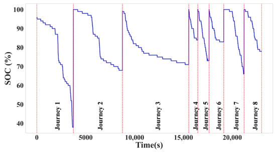
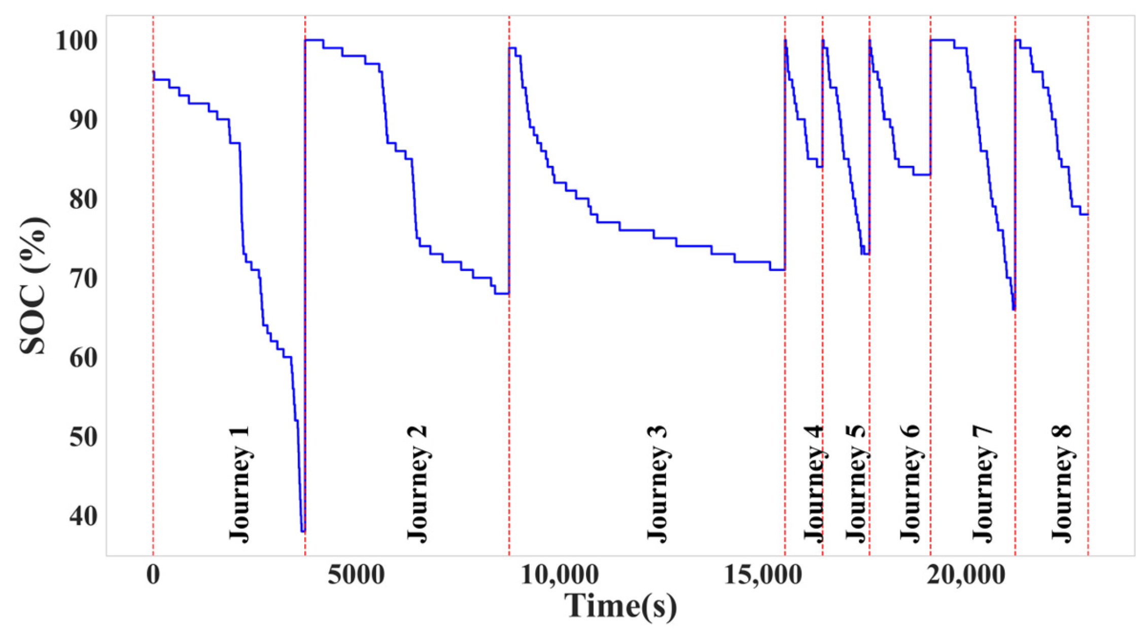
The data were divided into various driving segments based on battery SOC change characteristics and time jump values. The vehicle charging times and the start times of driving segments were determined based on SOC change patterns. Additionally, for segments with large time jumps (time jump interval greater than 140 s), the vehicle entering the next driving segment from the jump time was considered, using both methods to determine driving segments. Based on the separation of charging and discharging data, the vehicle discharge situation was segmented as shown in Figure 1 [18].

Figure 1. Discharge segment division.

2.2. Outlier Detection and Interpolation Processing

When the onboard data terminal dynamically acquires vehicle operating parameters, systematic deviations and hidden abnormal data can easily occur due to sensor failure, signal interference, data transmission errors, etc. The presence of these abnormal data may significantly impact the accuracy of vehicle cycle and energy consumption analysis, such as causing overestimation or underestimation of energy consumption, or deviations in extracting cycle characteristics. This study used the boxplot method to identify and process these abnormal data [19].

The definitions of the boxplot upper edge ${\mathrm{X}}_{\mathrm{U}}$ and lower edge ${\mathrm{X}}_{\mathrm{L}}$ are shown in formulas (1) and (2), where ${\mathrm{Q}}_{\mathrm{U}}$ is the upper quartile, and ${\mathrm{Q}}_{\mathrm{L}}$ is the lower quartile:

$$X_U=Q_U+1.5I$$

(1)

$$X_L=Q_L-1.5I$$

(2)

After screening the operational data of electric vehicles for outliers, the outliers are replaced with None. Since data during vehicle driving is crucial for cycle and energy consumption analysis, abnormal data cannot simply be deleted; instead, the abnormal data is filled. For abnormal data filling, this study used linear interpolation.

2.3. Data Smoothing Processing

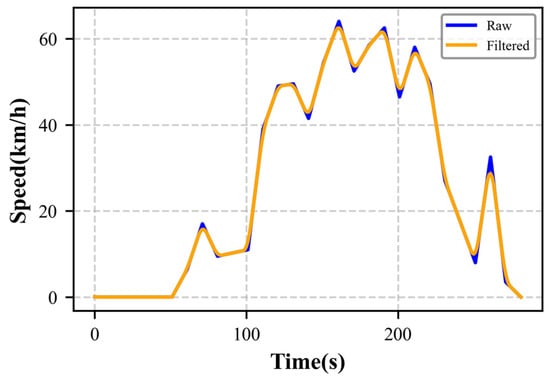
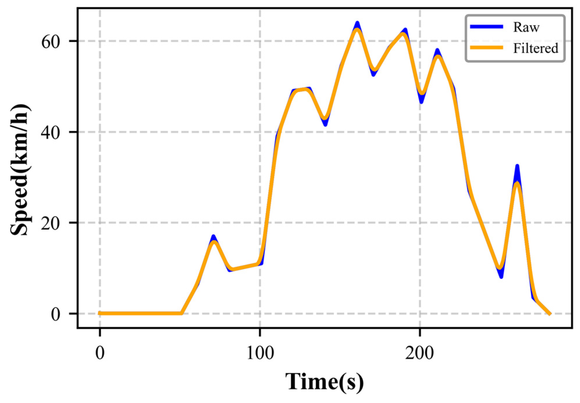
To mitigate random fluctuations in vehicle speed data caused by high-frequency measurement noise from sensors, a smoothing filtering method based on local weighted kernel regression was applied to the raw speed sequences. Specifically, the Epanechnikov parabolic kernel function was adopted as the weight assignment criterion, which is defined as

$$\mathrm{K}\left(\mathrm{u}\right)=0.75(1-{\mathrm{u}}^2)\hspace{1em}\left|\mathrm{u}\right|<1$$

(3)

The half-window width was set to h = 4, meaning that the sliding window encompassed the target point along with its four preceding and four succeeding consecutive sampling points, totaling nine points. For each neighboring point within the window, the kernel weight was first computed based on its normalized distance to the target point; all kernel weights within the window were then normalized to ensure they summed to unity, and the final filtered output for the target point was obtained as the weighted average of the measured speeds in the window. The filtering effect is shown in Figure 2.

Figure 2. Filtering effect comparison chart.

3. Vehicle Operating Data Analysis

3.1. Micro-Trip Division

Vehicle motion can be seen as a long-term motion composed of numerous short motion segments. Each short segment includes four states: acceleration, deceleration, idle, and constant speed. The definitions of each state are shown in Table 2.

Table 2. State definition table.

State	Speed (m/s)	Acceleration (m/s2)
Acceleration	—	≥0.15
Deceleration	—	≤0.15
Idle	<0.5	>−0.15 and <0.15
Constant Speed	≥0.5	>−0.15 and <0.15

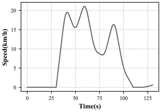
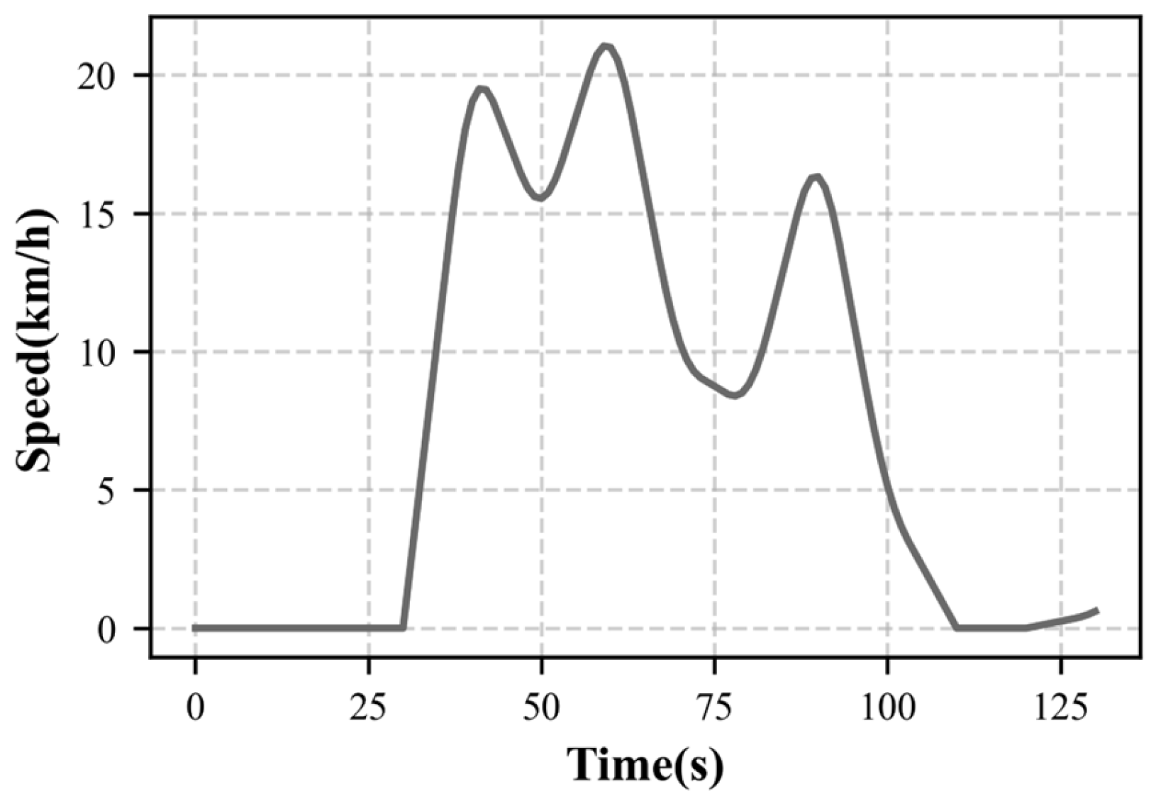
In this paper, a vehicle operation micro-trip is defined as starting from an idle state with a vehicle speed of 0, undergoing a series of speed changes, and entering a state with a vehicle speed of 0 again. A schematic diagram of a vehicle operation micro-trip is shown in Figure 3.

Figure 3. Schematic diagram of a driving micro-trip.

Acceleration was calculated from the vehicle speed using the time-difference method. The speed and the derived acceleration data were then used to identify and divide different driving states of the vehicle. Micro-trips containing idle states exceeding 180 s and micro-trips with excessively short duration were regarded as erroneous micro-trips and removed. A total of 6371 micro-trips were extracted.

3.2. Feature Parameter Construction

To comprehensively characterize the actual driving environment of electric vehicles, 16 feature parameters were selected for comprehensive evaluation in this study. These parameters were determined by referring to mature feature-selection strategies in existing driving cycle studies and combining the practical driving characteristics of household pure-electric vehicles in plain areas. All these features were calculated from vehicle speed, time, acceleration and vehicle operating-state data. Although several speed-related indicators, including average speed, running speed, maximum speed, and speed standard deviation, present statistical correlation, all features are retained completely. This strategy preserves all valid driving-characteristic information contained in the original data and avoids the loss of potential key features caused by manual screening. The selected indicators are shown in Table 3.

Table 3. Feature parameters of micro-trip segments.

Symbol	Definition	Unit
L	Travel Distance	m
s	Travel Time	s
Va	Average Speed	m/s
Vstd	Standard Deviation of Speed	m/s
Vmax	Maximum Speed	m/s
amax	Maximum Acceleration	m/s2
amin	Minimum Acceleration	m/s2
Vc	Average Running Speed	m/s
Vc-std	Standard Deviation of Running Speed	m/s
ahstd	Standard Deviation of Acceleration	m/s2
ahave	Average Acceleration	m/s2
adave	Average Deceleration	m/s2
Pa	Percentage of Acceleration Time	%
Ps	Percentage of Deceleration Time	%
Pc	Percentage of Constant Speed Time	%
Pi	Percentage of Idling Time	%

3.3. Principal Component Analysis

3.3.1. Principle of Principal Component Analysis

Principal component analysis is a commonly used data dimensionality reduction technique [20]. Its mathematical essence lies in constructing orthogonal linear mapping functions, mapping high-dimensional data to a low-dimensional space through linear transformation while preserving the main features of the data as much as possible. The principle is as follows: suppose the original observation dataset contains p-dimensional feature vectors and has a total of n driving segments, then an n × p dimensional driving cycle feature matrix can be formed, as shown in formula (4):

$$\mathit{X}=\left[\begin{array}{cccc}{x}_{11}& x_{12}& \cdots & x_{1p}\\ x_{21}& x_{22}& \cdots & x_{2p}\\ ⋮& ⋮& \ddots & ⋮\\ x_{n1}& x_{n2}& \cdots & x_{np}\end{array}\right]=\left(x_1,x_2,\cdots x_p\right)$$

(4)

Principal component analysis reduces the p dimensional data to m-dimensional data Z:{z₁, z₂, …, z_m}. The new variables fully reflect the main information of the original data according to the principle of retaining the main information content. In this way, the data dimension can be reduced while maximizing the retention of data variance.

The steps of principal component analysis are as follows:

(1)

Calculate the mean and standard deviation of the original data, and standardize the original data to reduce the influence of variable units:

$$\begin{array}{c}{\tilde{X}}_{ik}={\displaystyle \frac{X_{ik}-{\overline{X}}_k}{S_k}}\left(i=1,2,\dots ,n;k=1,2,\dots p\right)\\ S_k={\displaystyle \frac{1}{n-1}}{\displaystyle \sum {\left(X_{ik}-{\overline{X}}_k\right)}^2}\end{array}$$

(5)

In the formula, ${\overline{X}}_k$ is the mean of the $k$-th feature value, and $S_k$ is the standard deviation of the $k$-th feature.

(2)

Calculate the correlation matrix $R$ of the standardized data:

$$\mathit{R}=\left[\begin{array}{cccc}{\mathrm{r}}_{11}& r_{12}& \cdots & r_{1p}\\ r_{21}& r_{22}& \cdots & r_{2p}\\ ⋮& ⋮& \ddots & ⋮\\ r_{p1}& r_{p2}& \cdots & r_{pp}\end{array}\right]$$

(6)

In the formula, $r_{ij}$ is the correlation coefficient between the $i$-th feature and the $j$-th feature, calculated as

$$r_{ij}={\displaystyle \frac{1}{n-1}}{\displaystyle \sum _{k=1}^n{X}_{ki}{X}_{kj}}$$

(7)

(3)

Calculate the eigenvalues and eigenvectors of the correlation matrix $R$: Arrange the obtained eigenvalues in descending order λ₁ ≥ λ₂ ≥ … ≥ λ_p ≥ 0. Each eigenvector is a unit vector:

$$\left\{\begin{array}{c}{y}_1=l_{11}{\tilde{x}}_1+l_{12}{\tilde{x}}_2+\cdots +l_{1p}{\tilde{x}}_p\\ y_2=l_{21}{\tilde{x}}_1+l_{22}{\tilde{x}}_2+\cdots +l_{2p}{\tilde{x}}_p\\ y_m=l_{m1}{\tilde{x}}_1+l_{m2}{\tilde{x}}_2+\cdots +l_{mp}{\tilde{x}}_p\end{array}\right.$$

(8)

(4)

Calculate the contribution rate b_i of each principal component and the cumulative contribution rate α_p:

$$\begin{array}{c}{b}_i={\displaystyle \frac{{\lambda }_i}{{\displaystyle \sum _{k=1}^p{\lambda }_k}}}(i=1,2,\dots ,p)\\ {\alpha }_p={\displaystyle \frac{{\displaystyle \sum _{k=1}^i{\lambda }_i}}{{\displaystyle \sum _{k=1}^p{\lambda }_k}}}(i=1,2,\dots ,p)\end{array}$$

(9)

(5)

Select principal components: During the dimensionality reduction process, it is usually necessary to balance the need for information retention and dimension compression. The number of retained principal components depends on the proportion of the cumulative variance they represent to the total variance. Generally, principal components with a cumulative variance contribution rate of over 80% are selected.

3.3.2. Principal Component Analysis Results

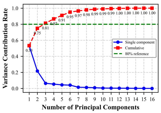
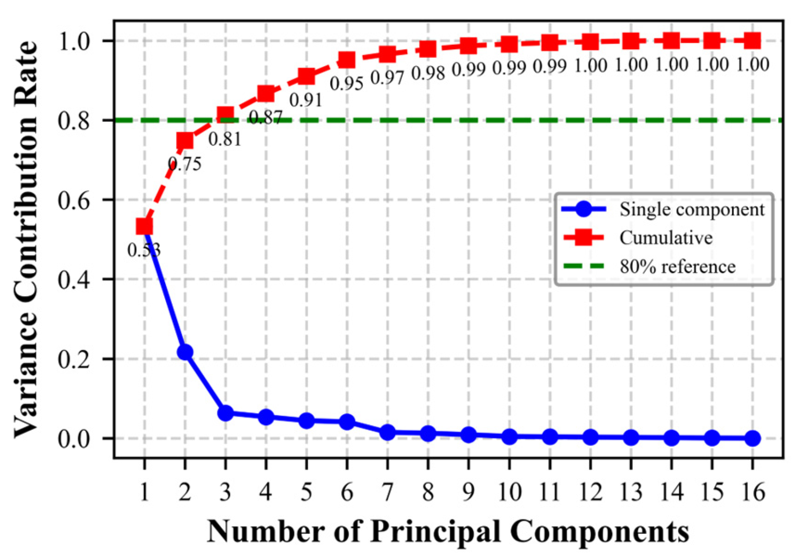
The method of principal component analysis was used to conduct an in-depth analysis of the 16 indicators extracted from the vehicle driving data. First, the data was standardized, and then the variance contribution rate and cumulative variance contribution rate of each principal component were calculated. The specific calculation results are shown in Table 4, and the principal component variance contribution rate and scree plot are shown in Figure 4.

Table 4. Micro-trip principal component information.

Principal Component (PC)	Variance	Variance Contribution Rate	Cumulative Variance Contribution Rate
1	8.52	53.25	53.25
2	3.46	21.63	74.88
3	1.02	6.36	81.25
4	0.86	5.37	86.62
5	0.70	4.39	91.00
6	0.66	4.10	95.11
7	0.23	1.46	96.57
8	0.20	1.23	97.80
9	0.14	0.87	98.67
10	0.07	0.43	99.09
11	0.05	0.33	99.43
12	0.04	0.24	99.67
13	0.03	0.19	99.86
14	0.02	0.11	99.97
15	0.00	0.03	100.00
16	0.00	0.00	100.00

Figure 4. Principal component variance contribution rate and scree plot.

From Table 4, it can be seen that the variances of the first three principal components are all greater than 1, and the cumulative variance contribution rate reaches 81.25%, containing the vast majority of information from the 16 feature values. Therefore, the first three principal components were extracted to represent the original feature parameters. Table 4 shows the load correlation distribution between the three selected principal components and the feature parameters.

From Table 5, it can be seen that the features with greater influence in the first principal component are maximum speed, speed standard deviation, running speed standard deviation, running speed, and average speed; the most influential in the second principal component are idle time proportion, travel time, and travel distance; the most influential in the third principal component is constant speed time proportion.

Table 5. Feature parameter factor loading matrix table.

Characteristic Parameter	PC1	PC2	PC3
Travel Distance (m)	0.383	0.774	0.046
Travel Time (s)	0.309	0.803	0.049
Average Speed (m/s)	0.833	0.446	−0.049
Standard Deviation of Speed (m/s)	0.894	−0.004	0.255
Maximum Speed (m/s)	0.928	0.262	0.129
Maximum Acceleration (m/s2)	0.805	−0.144	0.040
Minimum Acceleration (m/s2)	−0.817	0.031	−0.234
Average Running Speed (m/s)	0.875	0.336	0.115
Standard Deviation of Running Speed (m/s)	0.895	0.004	0.205
Standard Deviation of Acceleration (m/s2)	0.815	−0.519	−0.057
Average Acceleration (m/s2)	0.661	−0.442	−0.009
Average Deceleration (m/s2)	−0.737	0.339	−0.220
Percentage of Acceleration Time (%)	0.720	−0.453	−0.308
Percentage of Deceleration Time (%)	0.645	−0.472	−0.479
Percentage of Idling Time (%)	−0.678	−0.344	0.605
Percentage of Constant Speed Time (%)	0.063	0.830	−0.276

3.4. Cluster Analysis

In data analysis, clustering is a common unsupervised learning method used to group similar objects into the same category. It can automatically partition data objects into multiple categories or clusters by mining the internal structure and patterns of the data without prior knowledge or label information. Objects within a cluster have high similarity, while objects between clusters show significant differences. The clustering method used in the study is k-means++ clustering.

3.4.1. Clustering Principle and Process

K-means clustering is an iterative optimization algorithm aimed at partitioning n objects in a dataset into k clusters, minimizing the sum of distances from each object to its belonging cluster center, using Euclidean distance as the measure [21]. The K-means clustering algorithm continuously adjusts the cluster centers to make objects within the same cluster tighter and objects between different clusters more dispersed. K-means++ is an improved version that optimizes the selection of initial cluster centers, improves clustering quality, reduces the impact of randomness, speeds up convergence, and reduces the risk of falling into local optima [22]. The execution of the K-means++ algorithm typically includes the following steps:

(1)

Initialization

• Initial center selection: First, a sample point is randomly selected from the dataset as the first cluster center.
• Determination of subsequent cluster centers: For each sample not yet selected, its minimum distance to all currently selected cluster centers is calculated. Let the minimum distance from data point Xi to the selected cluster centers be D(x_i). The next center point is selected according to a probability distribution where the probability of each point being selected is proportional to the square of its minimum distance, as shown in Formula (10):

  $$P\left(x_i\right)={\displaystyle \frac{D{\left(x_i\right)}^2}{{\displaystyle {\sum }_{j}D{\left(x_i\right)}^2}}}$$

  (10)
  In the formula, $D\left(x_i\right)$ is the distance from the data point to the selected cluster centers, and $P\left(x_i\right)$ is the probability. The larger $P\left(x_i\right)$, the greater the probability that the point is selected as a cluster center.
• Step 2 is repeated until k cluster centers are selected.

(2)

Assignment

Each data point is assigned to the nearest cluster center based on the selected cluster centers. Euclidean distance is used as the distance measure between each data point and the cluster centers, and the data point is assigned to the nearest cluster center. The Euclidean distance calculation formula is shown in (11):

$$dist\left(x,c_i\right)=\sqrt{{{\displaystyle \sum _{j=1}^d\left(x_j-c_{ij}\right)}}^2}$$

(11)

In the formula, $x$ is the data point, $c_i$ is the i-th cluster center, $d$ is the data dimension, and x_j and c_ij are the values of x and c_i on the j-th dimension, respectively.

(3)

Update

The center of each cluster is updated and recalculated. The new cluster center is the mean of all data in that cluster, calculated as follows:

$$c_i={\displaystyle \frac{1}{\left|S_i\right|}}{\displaystyle \sum _{x\in S_i}x}$$

(12)

In the formula, S_i is the set of data points for the i-th cluster, and |S_i| is the number of data points in that set.

(4)

Iteration

The assignment is repeated and steps updated until the termination condition is met. The termination condition is that the cluster centers no longer change significantly.

3.4.2. Cluster Result Analysis

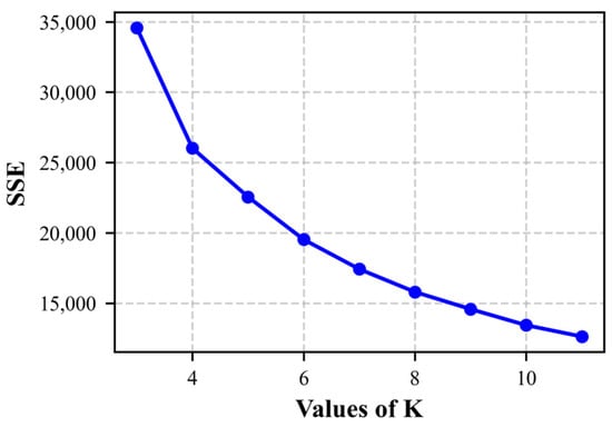
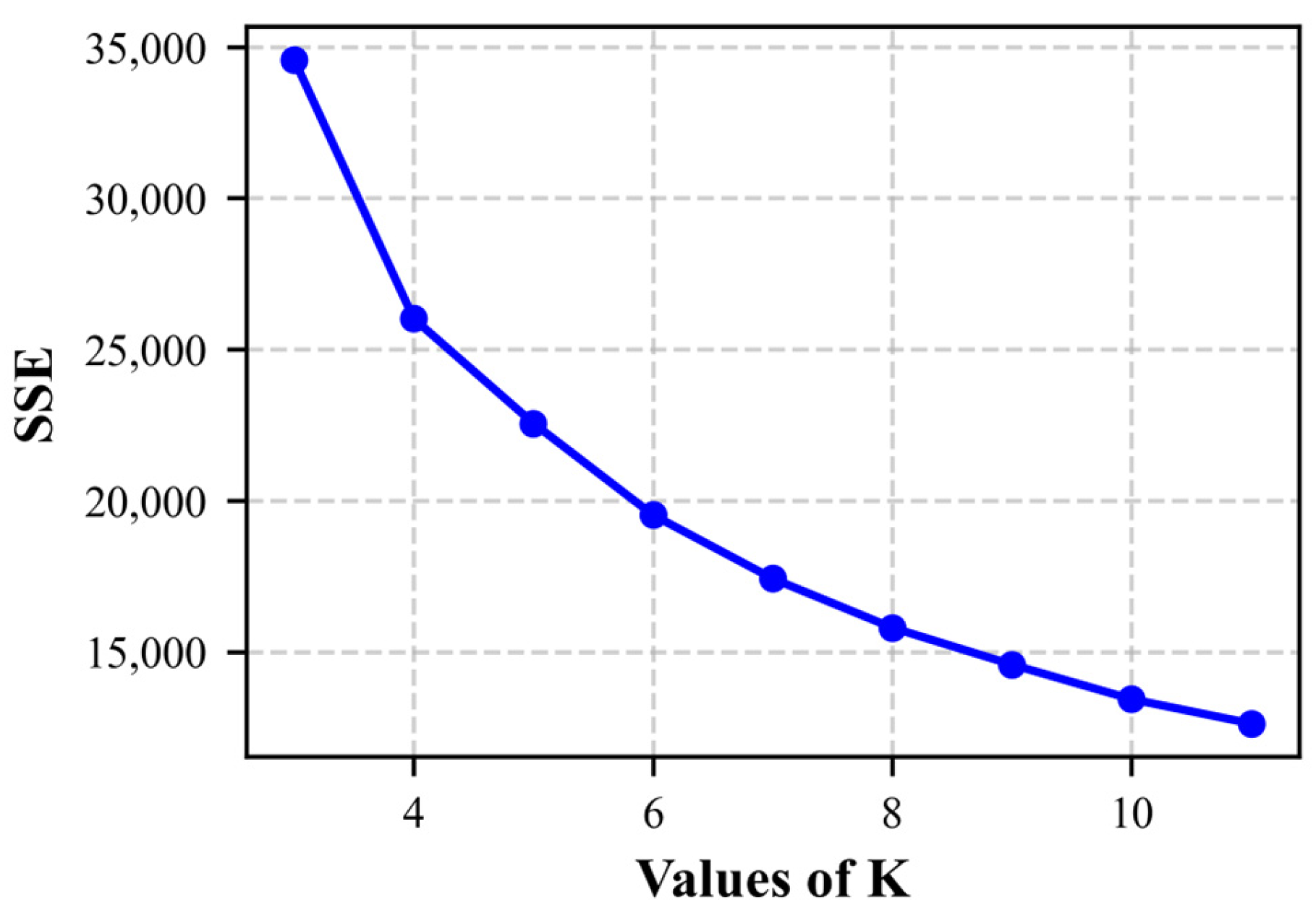
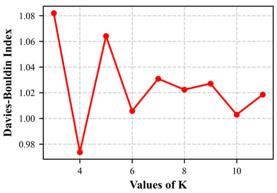
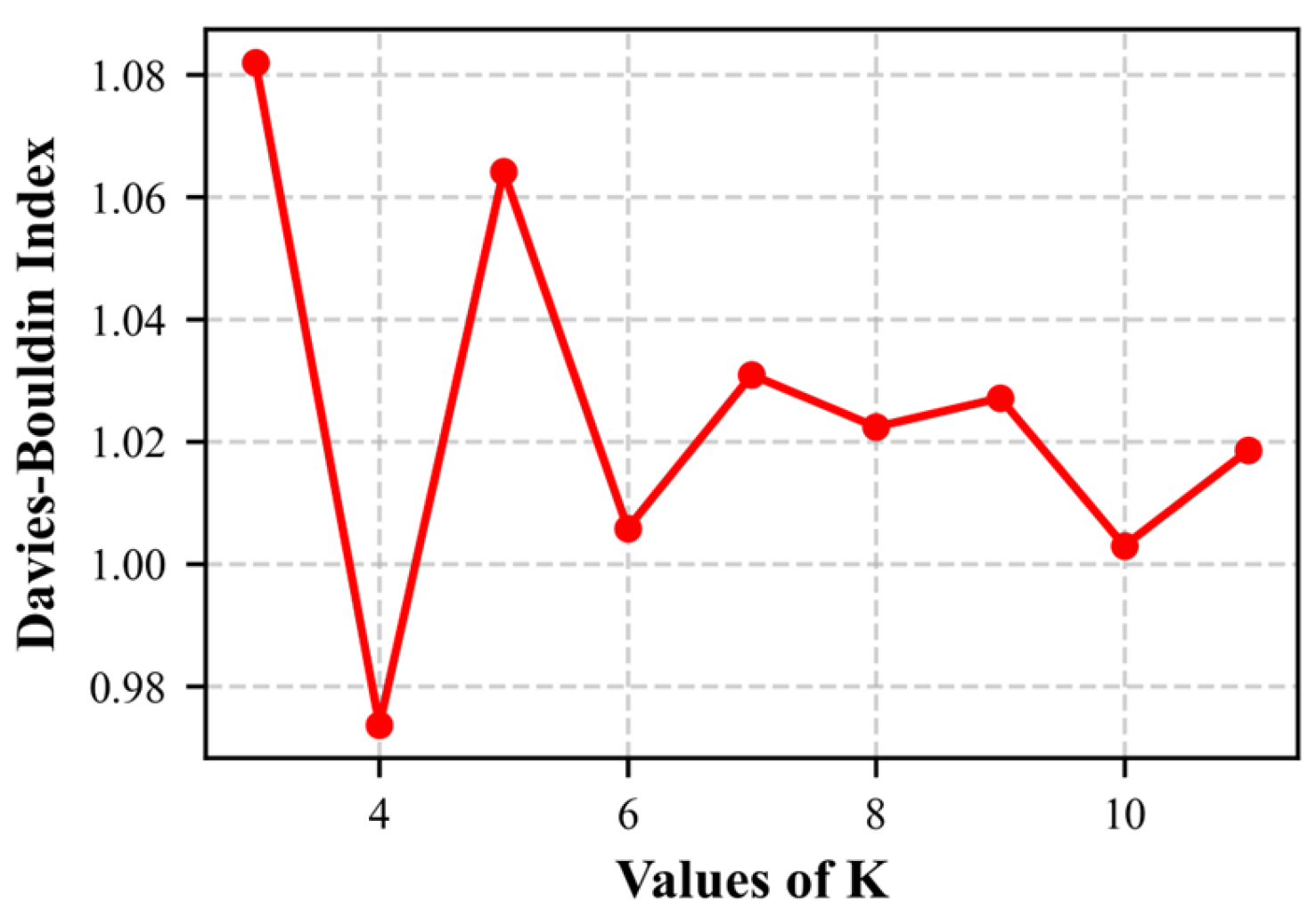
The number of clusters is an important factor affecting the clustering results. To ensure the rationality of the number of clusters, the study used the elbow method and the Davies–Bouldin (DB) Index method to jointly determine it. The elbow method can intuitively and qualitatively show the optimal number of clusters, while the DB index can be applied to clusters of different shapes, has high clustering quality, strong adaptability, and can quantitatively show the optimal number of clusters [23,24]. The details are as follows:

(1)

Elbow method: As the number of clusters k increases, the sample division becomes more refined, and the sum of squared errors (SSE) within each category gradually decreases. However, the decrease in SSE is not linear. After k increases to a certain extent, the rate of decrease in SSE gradually becomes smaller and tends to stabilize. This “bend” or “inflection point” is the elbow point. The elbow point indicates the number of clusters. The elbow method analysis is shown in Figure 5 [25].

$$SS{E}_i={\displaystyle \sum _{i=1}^k{\displaystyle \sum _{j=1}^{c_i}{\left|c_{ij}-\overline{c_i}\right|}^2}}$$

(13)

Figure 5. Elbow method analysis for number of clusters.

In the formula, c_ij is the j-th sample of the i-th class, and the latter is the mean of the samples of the i-th class.

(2)

DB method: The DB method is a standardized method used to evaluate clustering quality, based on an internal evaluation index of within-cluster distance and between-cluster distance. A smaller value indicates better clustering effect. The DB method can handle clusters of different sizes and densities well and has strong robustness to noise and outliers [26]. It is suitable for evaluating clustering results with different numbers of clusters. The DB method analysis is shown in Figure 6.

$$DB={\displaystyle \frac{\mathrm{avg}\left(s_i\right)-avg\left(s_j\right)}{d(C,D)}}$$

(14)

Figure 6. DB method analysis for number of clusters.

In the formula, S_i and S_j are the distances from the data samples in class C and class D to their respective cluster centers. d(C, D) is the distance between the center points of class C and class D. The maximum value of all DB analyses was taken to obtain the final value.

From the elbow method analysis, it can be seen that when k < 4, the SSE decreases rapidly, and after k > 4, the rate of decrease in SSE tends to flatten, with the inflection point at 4, so 4 classes should be selected. Meanwhile, the analysis from the DB coefficient in Figure 6 shows that when the number of clusters is 4, the DB coefficient reaches the minimum value, so 4 classes should be selected. Considering both, k = 4 was finally selected as the optimal number of clusters.

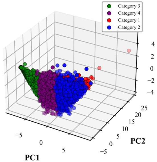
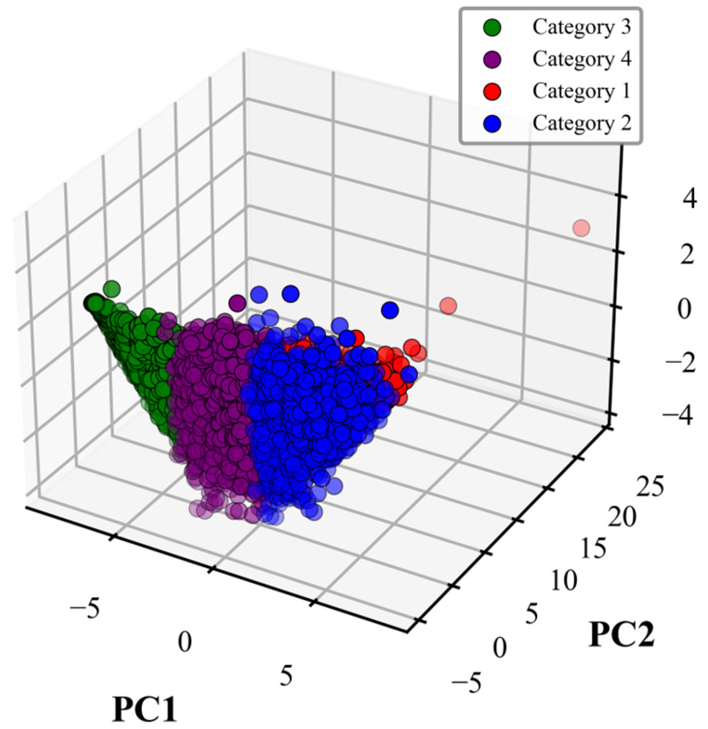
The results of the 4 clusters were plotted and are shown in Figure 7.

Figure 7. Micro-trip cluster chart.

In Figure 7, different colors represent different cycles. Analysis of the figure shows that the micro-trips are well classified, with significant differences between clusters, indicating a good clustering effect [27]. To more specifically show the characteristics of each cluster, the 16 features for each cluster are displayed in Table 6, which shows the mean values of the feature values for each type of cycle after clustering.

Table 6. Mean feature parameters for each cluster.

Characteristic Parameters	Category 1	Category 2	Category 3	Category 4
Travel Distance (m)	103.37	869.53	2332.09	7540.92
Travel Time (s)	119.58	195.01	268.66	786.35
Average Speed (m/s)	0.78	4.04	8.12	9.31
Standard Deviation of Speed (m/s)	0.75	3.20	5.16	4.21
Maximum Speed (m/s)	2.46	9.75	15.97	15.89
Maximum Acceleration (m/s2)	0.18	0.53	0.72	0.58
Minimum Acceleration (m/s2)	−0.18	−0.59	−0.92	−0.75
Average Running Speed (m/s)	1.17	5.19	9.41	9.86
Standard Deviation of Running Speed (m/s)	0.72	2.84	4.49	3.73
Standard Deviation of Acceleration (m/s2)	0.08	0.24	0.35	0.21
Average Acceleration (m/s2)	0.13	0.34	0.38	0.29
Average Deceleration (m/s2)	−0.13	−0.37	−0.47	−0.34
Percentage of Acceleration Time (%)	5.78	21.93	30.46	17.52
Percentage of Deceleration Time (%)	5.31	20.67	25.49	15.50
Percentage of Idling Time (%)	56.58	26.29	15.35	6.52
Percentage of Constant Speed Time (%)	32.32	31.11	28.70	60.46

3.5. Operating Environment Analysis

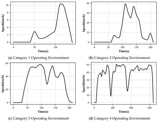
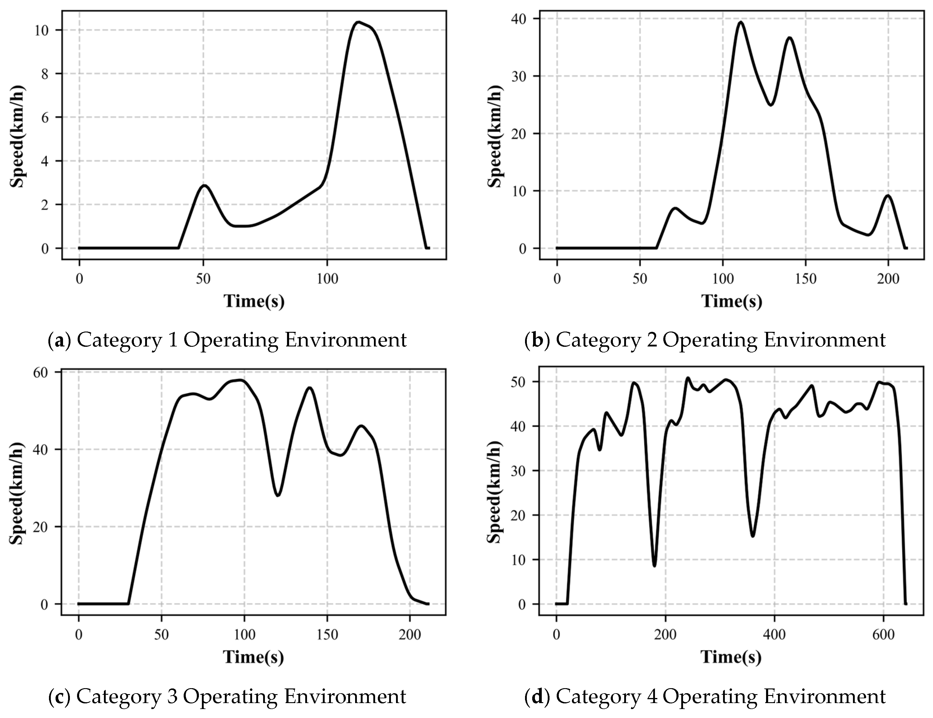
From Table 6, it can be seen that under Category 1 cycle conditions, denoted as the congested-urban condition, the travel mileage is low, the running time is short, the vehicle’s average speed is the lowest, and the idle time proportion is the highest, while the acceleration and deceleration time proportions are very small. This indicates that the vehicle may be on urban roads or in congested conditions. Under Category 2 cycle conditions, denoted as the urban-arterial condition, the speed, mileage, and velocity increase, and both the acceleration and deceleration time proportions significantly improve, while the idle state time greatly decreases, with little stagnation, indicating relatively smooth operation. This suggests that this cycle represents medium-speed driving, possibly corresponding to suburban roads, ring roads, or relatively unimpeded urban arterial roads.

Category 3 represents a medium-high speed driving mode, denoted as the suburban condition, where speed and mileage are both higher than in Category 2, and the idle state further decreases. Category 4 represents high-speed driving conditions, denoted as the high-speed condition. In this category, the idle proportion is the smallest, the constant speed proportion is the largest, and both speed and mileage are the highest, indicating that this cycle likely involves driving on highways or roads with sparse traffic. The speed curves of the four types of cycles are shown in Figure 8.

Figure 8. Different categories of operating environments.

4. Driving Cycle Construction

4.1. Cycle Construction

From the clustering algorithm used in the study, it is known that the closer each micro-trip segment is to its cluster center, the more it can represent the characteristics of that type of cycle. Referring to domestic and international cycle construction tests, cycle construction is generally around 1800 s. The study aims for this duration for cycle construction. Therefore, the following steps were used to screen micro-trip segments and complete the cycle construction:

(1)

The various short segments for the 4 cycle categories were sorted based on their distance to the corresponding cluster center.

(2)

The total duration of each of the 4 cycle categories was calculated to determine their respective proportions, thereby obtaining the time for each cycle type in the typical cycle.

(3)

Based on the ideal time for each cycle, the micro-trip segments were screened within their respective types that met the duration requirement.

(4)

The cycle segments were spliced.

According to the above-mentioned conditions, to construct an ideal driving cycle of 1800 s, the target total durations allocated to the four types of driving cycles under ideal conditions are as follows: low-speed cycle 80 s (4.44%), medium-speed cycle 339 s (18.83%), medium-high-speed cycle 463 s (25.72%), and high-speed cycle 917 s (50.94%).

However, limited candidate micro-trips are close to each cluster center, and their actual durations cannot fully match the target durations. Therefore, for the selection of micro-trips for each cluster, the micro-trip duration was constrained so as to not exceed the ideal target duration on the premise of selecting segments according to their distances to the cluster center.

The finally selected micro-trips are shown in Table 7.

Table 7. Micro-trip segment information.

Cycle Type	Segment Category	Segment ID	Distance to Cluster Center	Distance-Based Rank	Segment Duration (s)
Low-speed cycle	congested-urban condition	3268	0.22	1	101
Medium-speed cycle	urban-arterial condition	3477	0.20	1	211
Medium-speed cycle	urban-arterial condition	3407	0.25	2	191
Medium-high-speed cycle	suburban condition	2548	0.26	7	381
High-speed cycle	high-speed condition	1661	0.15	1	641
High-speed cycle	high-speed condition	398	0.19	2	461

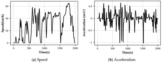
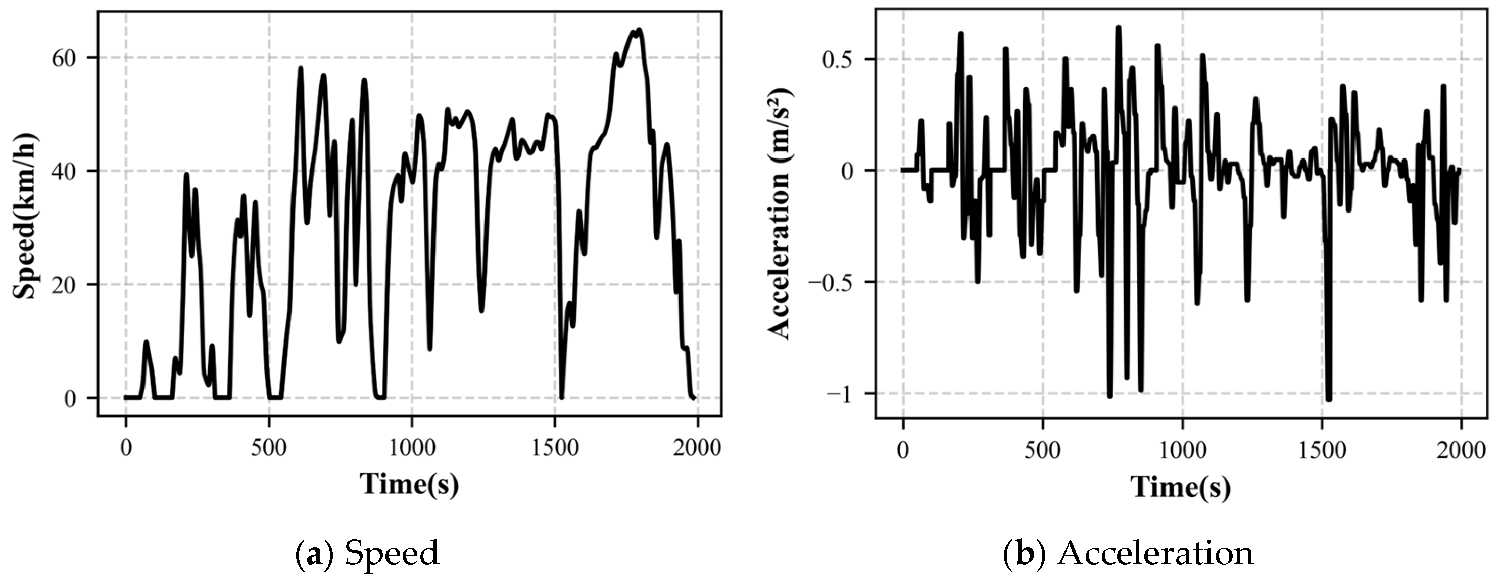
For the medium-high-speed category, the top-6 candidate micro-trips ranked by distance exceeded the ideal target duration; thus, the 7th-ranked segment satisfying the duration constraint was selected. Finally, a driving cycle for pure-electric passenger vehicles was constructed, with a total duration of 1986 s, a maximum speed of 64.80 km/h and a travel distance of 16.67 km. The schematic diagram of the spliced driving cycle is presented in Figure 9.

Figure 9. The constructed driving cycle.

4.2. Cycle Comparison

The accuracy of the constructed driving cycle needs to be compared with the state of the original data to ensure its representativeness.

The study selected 10 commonly used indicators to compare the typical cycle with the original data, thereby ensuring the completeness and representativeness of the typical cycle in various aspects. The relative error was adopted to quantify the discrepancy between the two, and its formula is presented as follows:

$$\mathrm{RE}={\displaystyle \frac{x_i-y_i}{y_i}}\times 100\%$$

(15)

In the formula, $x_i$ denotes each state-related indicator of the constructed driving cycle, and $y_i$ represents each corresponding indicator of the reference driving-cycle dataset.

The comparison information is shown in Table 8 below.

Table 8. Comparison of cycle characteristic parameters.

Characteristic Parameters	Driving Cycle	Raw Data	Relative Error
Average Speed (m/s)	8.39	7.99	5.00%
Standard Deviation of Speed (m/s)	5.37	5.39	−0.44%
Average Running Speed (m/s)	9.50	8.99	5.78%
Standard Deviation of Acceleration (m/s2)	0.24	0.25	−3.32%
Average Acceleration (m/s2)	0.30	0.32	−6.44%
Average Deceleration (m/s2)	−0.38	−0.37	1.83%
Percentage of Acceleration Time (%)	21.06	20.48	2.81%
Percentage of Deceleration Time (%)	17.28	17.94	−3.71%
Percentage of Idling Time (%)	13.15	13.57	−3.11%
Percentage of Constant Speed Time (%)	48.51	48.00	1.07%

Analysis of Table 8 shows that the relative errors between the constructed driving cycle and the original vehicle driving data for the 10 commonly used indicators are all small, mostly below 5.00%. Among them, acceleration proportion, deceleration proportion, idle proportion, and constant speed proportion are important parameters showing the vehicle operating state. The relative errors of these four items are all within 4.00%, indicating the reasonableness of the operating state of the constructed cycle.

To more comprehensively measure the difference between the driving cycle and the real cycle, the average value of the absolute values of the relative errors of the 10 indicators was calculated to be 3.35%, which is a small error, indicating that the constructed cycle can accurately reflect the driving cycle of pure electric passenger vehicles.

5. Discussion

This study implements a typical driving-cycle construction workflow combining real-world operational data, PCA dimensionality reduction and K-means++ clustering. Although PCA and K-means++ are well-established algorithms, the added value of this work lies not in the invention of new clustering tools. Instead, this study further interprets each clustered micro-trip group against real-world traffic conditions, distinguishing congested urban, arterial-road, suburban and highway driving scenarios. Different from most existing studies that only output speed-time sequences, this work links micro-trip statistical features with practical road-traffic environments, which provides clearer physical interpretation for the obtained driving-cycle segments.

Comparisons between the constructed cycle and international typical certification driving cycles are summarized in Table 9. Noticeable parameter gaps exist between standard certification cycles and the regional cycle proposed herein. As generalized nationwide or global type-approval tools, CLTC-P, NEDC, and WLTC are designed to cover broad traffic scenarios and cannot fully capture local usage patterns of household PEPVs in plain-area regions of China. In contrast, the present cycle reflects statistical characteristics derived from local real-world vehicle telematics data, exhibiting distinct proportions of idle, acceleration, deceleration, and constant-speed phases. These discrepancies underline the necessity of building region-specific driving cycles for local-targeted energy-consumption simulation and driving-range evaluation.

Table 9. Comparison with international typical certification driving cycles.

Characteristic Indicators	Constructed Driving Cycle	CLTC-P	Relative Error vs. CLTC-P	NEDC	Relative Error vs. NEDC	WLTC	Relative Error vs. WLTC
Average speed (km/h)	30.20	28.96	4.30%	33.6	−10.11%	46.4	−34.91%
Running speed (km/h)	34.2	37.18	−8.02%	43.5	−21.38%	53.2	−35.71%
Mean acceleration (m/s2)	0.3	0.45	−33.33%	0.53	−43.40%	0.53	−43.40%
Mean deceleration (m/s2)	−0.38	−0.49	−22.45%	−0.75	−49.33%	−0.58	−34.48%
Acceleration time proportion (%)	21.06	28.61	−26.39%	23.2	−9.22%	30.9	−31.84%
Deceleration time proportion (%)	17.28	26.44	−34.64%	16.6	4.10%	28.6	−39.58%
Idle time proportion (%)	13.15	22.11	−40.52%	22.6	−41.81%	12.7	3.54%
Constant-speed time proportion (%)	48.51	22.83	112.48%	37.5	29.36%	27.8	74.50%

Driving-cycle characteristics exert direct impacts on electric-vehicle energy-consumption assessment. Higher idle fractions and frequent acceleration-deceleration events tend to raise simulated energy consumption, whereas prolonged constant-speed segments reduce transient power demands. Mismatch between driving-cycle parameters and real-world statistical distributions introduces bias in energy-consumption and driving-range estimation. Therefore, the representative regional driving cycle constructed in this work can mitigate such bias for vehicle simulation and energy-management strategy evaluation.

Further cross-comparison against previously published regional driving cycles for Chinese cities is provided in Table 10.

Table 10. Comparison with typical driving cycles of Chinese cities.

Characteristic Indicators	Constructed Driving Cycle	Chongqing	Tianjin	Qingdao
Average speed (km/h)	30.20	16.22	23.57	20.51
Running speed (km/h)	34.2	22.55	31.03	29.8
Mean acceleration (m/s2)	0.3	0.62	0.86	0.66
Mean deceleration (m/s2)	−0.38	−0.66	−0.89	−0.65
Acceleration time proportion (%)	21.06	27.78	30.72	23.88
Deceleration time proportion (%)	17.28	27.08	30.00	24.12
Idle time proportion (%)	13.15	28.54	22.89	31.17
Constant-speed time proportion (%)	48.51	16.62	16.39	20.84

Marked inter-study differences can be observed across these city-specific cycles. The mountain-city cycle for Chongqing shows low average speed and substantially elevated idle-time fraction, reflecting frequent stop-and-go traffic induced by complex terrain. Cycles from Tianjin and Qingdao exhibit moderate average speed and high idle proportions under coastal-urban traffic conditions. By comparison, our plain-area dataset yields distinctly higher constant-speed fractions and lower idle ratios. These divergences further demonstrate that geography and local traffic patterns strongly shape driving-cycle statistics, reinforcing the necessity of developing region-adapted driving cycles for PEPV research.

This work targets vehicle-level simulation and energy-management strategy development for automotive engineering applications, rather than providing analytical tools for public-policy formulation. Several limitations should also be acknowledged. The dataset only covers household electric vehicles operating in plain regions. Direct ground-truth information, including road type, traffic-congestion level, weather conditions, driver characteristics and precise city-level geographic coordinates, is unavailable from the telematics dataset. Accordingly, the operating-environment categories in this study were statistically inferred from micro-trip features instead of real-world GIS labels. Road-gradient information is also not involved in feature extraction. Future research can incorporate road-slope parameters, multi-source geographic and meteorological data, and expand datasets covering diversified geographic conditions to further generalize the proposed method.

6. Conclusions

To improve the performance evaluation of electric vehicles, such as in the fields of range prediction, fatigue simulation, and software/hardware parameter tuning, this paper, targeting data from ordinary household PEPV driving in plain areas, studied four typical vehicle operating environments combined with the micro-trip method and constructed a driving cycle. The main conclusions are as follows:

The operating modes of PEPVs are mainly divided into four categories: In the first type of cycle mode, the vehicle speed is low, and the idle proportion is large, representing congested road conditions. In the second type of cycle mode, the vehicle speed increases slightly, the idle proportion decreases, and the acceleration/deceleration proportions increase, mostly representing urban arterial road conditions. In the third mode, the vehicle speed further increases, and traffic is relatively smooth, representing typical suburban conditions. In the fourth type of cycle mode, the vehicle speed is the highest, with little low-speed stagnation, and the constant speed state occupies the majority, representing typical highway conditions.

By comparing the driving cycle with the original data, the comprehensive average error is 3.35%, indicating that the typical cycle can largely reproduce the actual driving characteristics of pure electric passenger vehicles, accurately reflect the vehicle’s operating state in daily complex traffic environments, and ensure its application accuracy in vehicle performance evaluation and other aspects.

The constructed driving cycle not only reflects the four operating modes of the vehicle but also has high construction accuracy, which can provide an effective reference for improving the economy of electric vehicles.

References

- Enayati, E.; Siavashi, M.; Mousavi, S.; Moaveni, A. Developing the optimal cooling strategy for battery thermal management systems under realistic driving conditions. Int. Commun. Heat Mass Transf. 2025, 162, 108589. [Google Scholar] [CrossRef] [Scilit]
- Liu, G.; Xu, J.N.; Chen, T.Y.; Zhang, B.L. Modeling and control simulation of integrated heating system for power batteries. J. Chongqing Jiaotong Univ. (Nat. Sci.) 2025, 44, 120–126. [Google Scholar]
- Liu, Y.; Wu, Z.X.; Li, M.L.; Yu, H.Z.N.; Wang, Y.; He, K.X.; An, X.P. Construction of driving cycles for passenger cars in China. J. Transp. Syst. Eng. Inf. Technol. 2020, 20, 233–240. [Google Scholar]
- Huang, C. Research on the Construction of Urban Driving Cycles for Electric Vehicles and Driving Style Recognition. Master’s Thesis, Chongqing University of Technology, Chongqing, China, 2022. [Google Scholar] [CrossRef]
- Wang, J.G.; Xu, H.; Liu, H. Construction of electric vehicle driving cycles based on t-SNE and fuzzy clustering. J. Chongqing Jiaotong Univ. (Nat. Sci.) 2022, 41, 126–132. [Google Scholar]
- Liang, R.; He, J.; Lu, P. Construction of Battery Electric Vehicle Driving Cycles Based on Improved Grey Wolf Optimized K-Means Clustering: A Case Study for Qingdao, China. World Electr. Veh. J. 2026, 17, 56. [Google Scholar] [CrossRef] [Scilit]
- Zhao, Z.C.; Sun, X.L.; Wang, X.; Wang, Y.; Fu, J.; Liu, J. Construction and optimization of representative actual driving cycles based on the improved autoencoder. Sci. Rep. 2024, 14, 2351. [Google Scholar] [CrossRef] [Scilit]
- Shi, J.; Zheng, W.; Huo, R.; Hong, P.; Li, B.; Ming, P. A Reinforcement Learning and Unsupervised Clustering-Based Method for Automated Driving Cycle Construction for Fuel Cell Light-Duty Trucks. World Electr. Veh. J. 2026, 17, 213. [Google Scholar] [CrossRef] [Scilit]
- Cao, Q.; Li, J.; Liu, Y.; Qu, D.-W. Construction of driving cycle based on big data and Markov chain. J. Northeast. Univ. (Nat. Sci.) 2019, 40, 77. [Google Scholar]
- Mafi, S.; Kakaee, A.; Mashadi, B.; Moosavian, A.; Abdolmaleki, S.; Rezaei, M. Developing local driving cycle for accurate vehicular CO2 monitoring: A case study of Tehran. J. Clean. Prod. 2022, 336, 130176. [Google Scholar] [CrossRef] [Scilit]
- Lee, S.; Eom, I.; Lee, B.; Won, J. Driving characteristics analysis method based on real-world driving data. Energies 2023, 17, 185. [Google Scholar] [CrossRef] [Scilit]
- Zhou, Y.Y.; He, L.; Chen, J.D.; Liu, D.; Zhang, J. DC-MPAM: A novel customized driving cycle construction method for predicting cruising distance and vehicle speed. IEEE Trans. Transp. Electrif. 2024, 10, 10481–10496. [Google Scholar] [CrossRef] [Scilit]
- Xu, N.; Liu, Q.; Yuan, C.; Yang, Y.; Kong, Y.; Jia, Y.; Li, L.; Li, J. A double-filter driving cycle generation framework with dynamometer testing and analysis. Transp. Res. Part D Transp. Environ. 2026, 153, 105231. [Google Scholar] [CrossRef] [Scilit]
- Türker, O.; Timo, L.; Heikki, S. Driver Behaviour Questionnaire: A follow-up study. Accid. Anal. Prev. 2006, 38, 386–395. [Google Scholar] [CrossRef] [Scilit]
- Wallace, B.; Goubran, R.; Knoefel, F.; Marshall, S.; Porter, M.; Smith, A. Driver unique acceleration behaviours and stability over two years. In Proceedings of the 2016 IEEE International Congress on Big Data (BigData Congress); IEEE: New York, NY, USA, 2016; pp. 230–235. [Google Scholar] [CrossRef] [Scilit]
- Eng, J.N.; Devlin, N.K.; Ang, J.; Split, M.; Lyons, R.; Schultheis, M.T. Validity of self-reported driving: It all depends on how and when you ask. Transp. Res. Part F Psychol. Behav. 2026, 116, 103417. [Google Scholar] [CrossRef] [Scilit]
- Dong, B.B. Research on Range Estimation Methods for Electric Vehicles Based on Battery State and Driving Energy Consumption Prediction. Master’s Thesis, Chang’an University, Xi’an, China, 2023. [Google Scholar] [CrossRef]
- Qin, Y. Range Estimation of Electric Vehicles Based on Battery State and Driving Energy Consumption. Master’s Thesis, Chang’an University, Xi’an, China, 2023. [Google Scholar]
- Cong, S. Neural Network Theory and Application with MATLAB Toolbox, 3rd ed.; University of Science and Technology of China Press: Hefei, China, 2009. [Google Scholar]
- Jolliffe, I.T.; Cadima, J. Principal component analysis: A review and recent developments. Philos. Trans. R. Soc. A Math. Phys. Eng. Sci. 2016, 374, 20150202. [Google Scholar] [CrossRef] [Scilit]
- Liu, J.L.; Li, L.; Yu, J. Research on driving cycle construction method based on improved K-means clustering. Agric. Equip. Veh. Eng. 2023, 61, 105–109. [Google Scholar] [CrossRef]
- Liao, J.Y.; Wu, S.; Li, W.; Liu, A.L. Construction of driving cycles for light-duty vehicles based on k-means++ clustering. J. Wuhan Univ. Technol. (Transp. Sci. Eng.) 2021, 45, 378–383. [Google Scholar] [CrossRef]
- He, X.S.; He, F.; Yu, H.L. Initialization improvement and clustering quality evaluation of the K-means algorithm. J. Xi’an Polytech. Univ. 2024, 38, 114–123. [Google Scholar] [CrossRef]
- Han, R.; Shi, P.W.; Ding, Q.G.; Yu, C.H. Construction of driving cycles for light-duty vehicles on urban roads in Harbin. J. Transp. Sci. Technol. Econ. 2025, 27, 50–58. [Google Scholar] [CrossRef]
- Guo, J.; Xie, D.; Jiang, Y.; Li, Y. A novel construction and evaluation framework for driving cycle of electric vehicles based on energy consumption and emission analysis. Sustain. Cities Soc. 2024, 117, 105951. [Google Scholar] [CrossRef] [Scilit]
- Lee, G.; Yeon, J.; Kim, N.; Park, S. A comprehensive methodology for developing and evaluating driving cycles for electric vehicles using real-world data. eTransportation 2025, 24, 100409. [Google Scholar] [CrossRef] [Scilit]
- Boruah, A.; Pawar, D.S.; Jain, R.; Eregowda, T.; Mitra, K.; Chatterjee, P. Representative driving cycle-based framework to model indirect CO2 emissions from electric cars. Transp. Res. Part D Transp. Environ. 2025, 144, 104777. [Google Scholar] [CrossRef] [Scilit]
Disclaimer/Publisher’s Note: The statements, opinions and data contained in all publications are solely those of the individual author(s) and contributor(s) and not of MDPI and/or the editor(s). MDPI and/or the editor(s) disclaim responsibility for any injury to people or property resulting from any ideas, methods, instructions or products referred to in the content. |
© 2026 by the authors. Licensee MDPI, Basel, Switzerland. This article is an open access article distributed under the terms and conditions of the Creative Commons Attribution (CC BY) license.