


Abstract
Eight-wheel drive vehicles have many areas of use, such as military, logistics, firefighting, and disaster response. One of the key design requirements of an 8 × 8 vehicle is to achieve low turning radius at low speeds, without loss of stability and handling at high speeds. In this study, an 8 m turning radius is taken as a preliminary design objective of a 24-ton vehicle, and best handling performance is achieved for high speeds using simulations and the Taguchi Method. While achieving the 8 m turning radius, calculations are based on Akerman’s principle to calculate the turning angles of each wheel. The bicycle model was derived using motion equations, then implemented in MATLAB/Simulink (version 2023b) model to predict the slip angle for six degrees of sinusoidal steering input and a longitudinal speed of 72 kph. The effects of design parameters such as steering configuration and axle distances on slip and steering angle were investigated by design of experiments. With the help of ANOVA analysis performed using Minitab software (version 19), the relationship and optimized solutions were achieved to satisfy both minimum slip angle and steering stability. Minitab optimizer results conclude that Configuration 3 with L1 = 2.45 m, L2 = L3 = 0.8 m, and L4 = 2.3 m axle distances achieved a mean slip of 2.54 × 10⁻² radians delay during the sinusoidal maneuver of 4.19 × 10⁻³ radians at 20 m/s forward speed. Although the optimum solution is achieved with the third configuration, there is not a common solution to achieve both the lowest slip and the highest stability with the same set of design parameters. Finally, a CAD model of the first two axles is established using the software Solidworks (version 2025). A kinematics model including pitman arm, idle arm, and steering rods is designed and virtually validated using ADAMS/View (version 2025.1) multibody dynamics software.
1. Introduction
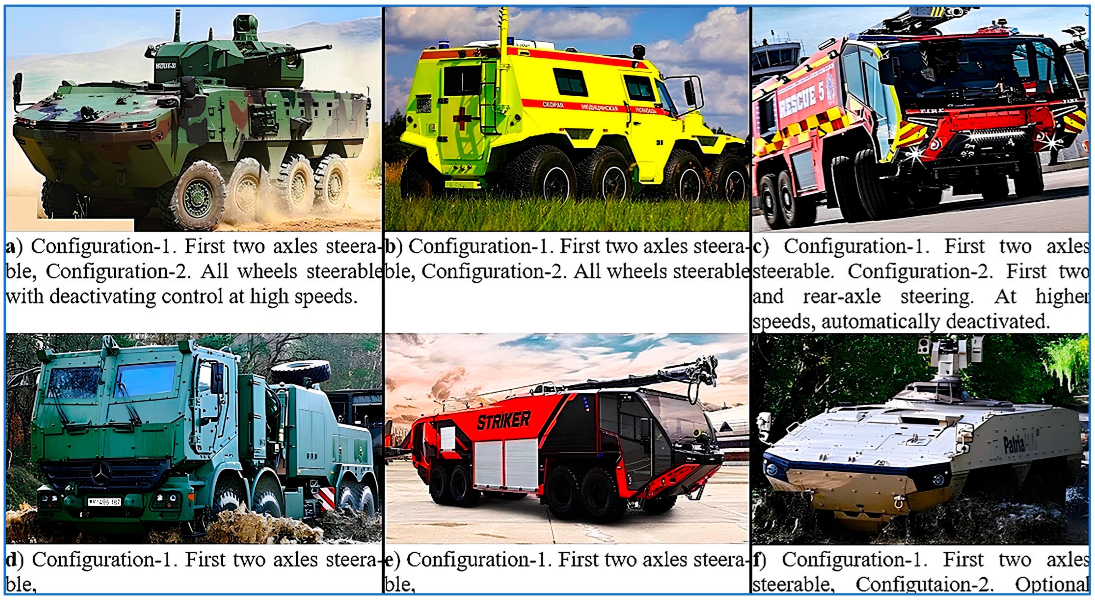
Eight-wheel drive vehicles are multi-axle vehicles that offer high mobility in various application areas, such as military, industrial, and emergency response. Eight-wheel drive vehicles provide balanced weight distribution and reduced ground pressure and allow vehicles to travel on off-road terrain [1,2,3,4]. Their robust chassis increases resistance to heavy loads and severe environmental conditions. Equipped with advanced suspension systems, these vehicles effectively absorb shocks and maintain stability and comfort on a variety of off-road conditions, such as bumpy terrain, mud, snow, and sand. In military operations, 8 × 8 vehicles are used for troop transportation, armored reconnaissance, and logistics support. Their ability to operate in diverse terrains and carry substantial payloads make them indispensable for defense forces [2]. In emergency and rescue operations, 8 × 8 vehicles are deployed to reach disaster areas, providing critical support and transportation. Therefore, they have a wide range of emergency uses, from responding to a forest fire to bringing hope to destroyed cities after an earthquake. In conclusion, 8 × 8 vehicles are specialized machines designed to perform extremely well in demanding environments where conventional vehicles might struggle. Their unique configuration, advanced features, and adaptability make them invaluable in various industries, despite the inherent challenges associated with their complexity and cost. Some of the 8 × 8 vehicles are presented in Figure 1.
Sophisticated steering systems, frequently with several steerable axles, are a feature of modern 8 × 8 vehicles that greatly reduce turning radius and improve maneuverability in limited areas. The drivetrain system is engineered to distribute torque evenly across all eight wheels, enhancing traction and stability. This feature is particularly useful in off-road scenarios where consistent power delivery to all wheels is crucial. When a multi-axle vehicle (MAV) is considered, there is always a conflicting performance of maneuverability and stability. Generally, active steering control systems and strategies were applied by many researchers to enhance both design requirements [5]. An et al. studied the linear quadratic linear regulator control method on a six-wheel steering system to improve maneuverability [6]. Checking vehicle performance with J-turn tests demonstrated that the control system can achieve a smaller turning radius and better stability. Zang et al. [7] introduced an adaptive yaw control scheme based on the estimation of the vehicle mass, yaw inertia, and center of gravity (CG) position. System parameters of these vehicles vary significantly due to varying conditions, such as unloading and full loading of payloads. Pareira et al. [8] proposed a trajectory tracking control strategy for a 6 × 6 armored vehicle based on a simplified dynamic model integrated with microprocessor controllers. The main objective of their study was to eliminate rollover risk during high-speed handling. Similar studies are also available for 8 × 8 vehicles. Active rear steering has been used in many research studies to enhance ground vehicles’ lateral stability. Ahmed et al. [9] worked on various controllers to actively steer the rear axles of a multi-axle combat vehicle using a linearized bicycle model. Bao et al. [10] proposed a coordinated slip control algorithm using the hierarchical linear quadratic regulator scheme for a 12 × 12 vehicle. The 12-wheel driving system was decoupled based on the wheel load and simplified to a double local subsystem.
In open literature, the second most widely studied topic for MAV is probably the synthesis of the steering system, including geometry and mechanisms. The effects of steering geometry on cornering have been frequently investigated by many researchers. Chen et al. [11] studied the effects of steering geometry and developed the proper steering mechanisms of a four-axle vehicle to improve cornering behaviors. It is concluded that fourth-axle steering can obviously cut down the turning radius and even the slip angle. Khang et al. [12] performed a valuable study to optimize the dimensional synthesis of Ackermann steering mechanisms for three-axle, six-wheeled vehicles. They employed optimization methods including particle swarm optimization, hybrid particle swarm optimization, differential evolution with golden ratio, and linear ensemble of parameters and mutation strategies in differential evolution.
In most studies, turning performance and steering stability were studied separately, while some of them are just focused on developing a steering mechanism to achieve low turning or cornering radius, and some of them worked to enhance handling performance by introducing complicated control algorithms [8,9,10,11,12,13,14,15]. The studies that take both design considerations into account are limited; therefore, it is worthwhile to analyze both of them [16,17,18] together.
Figure 1.
Military and industrial examples of 8 × 8 vehicles. (a) Otokar Arma armored vehicle [19], (b) Avtoros Shaman armored vehicle [20], (c) Rosenbauer Panther airport rescue and firefighting vehicle [21], (d) Mercedes Actros logistic truck [22], (e) Oshkosh Striker Airport fire fighter vehicle [23], (f) Patria AMV armored vehicle [24].
1.1. Mathematical Modeling of Steering
When a vehicle turns, all the wheels cover different angular displacements. At lower speeds, the extensions of the axes of the steered front wheels will intersect with the extension of the rear axle at the center of the curve without error. This situation is called the Ackerman principle [25,26]. Ackermann steering geometry is a basic principle in vehicle dynamics and focuses on increasing the steering efficiency of vehicles by reducing tire slip during cornering [25]. For 8 × 8 vehicles with four steerable axles, this principle is extended to ensure that all steerable wheels are correctly aligned. The steering angles for each axle must be calculated to ensure that all wheels are oriented towards the same turning center.
Achieving precise Ackermann geometry in 8 × 8 vehicles requires careful design and calibration of the steering linkages and steering control systems. Steering linkages are adjusted such that the calculated steering angles for each wheel are achieved during turning maneuvers. In 8 × 8 vehicles, all-wheel steering systems often incorporate Ackermann principles to optimize the steering angles for all steerable axles. By ensuring that all wheels follow concentric paths, the stability and control of the vehicle are significantly improved at low speeds. Implementing Ackermann geometry in 8 × 8 vehicles is more complex due to the need to coordinate multiple axles and their respective steering angles. Understanding slip helps to optimize steering response, improve vehicle stability, and increase overall handling performance [25].
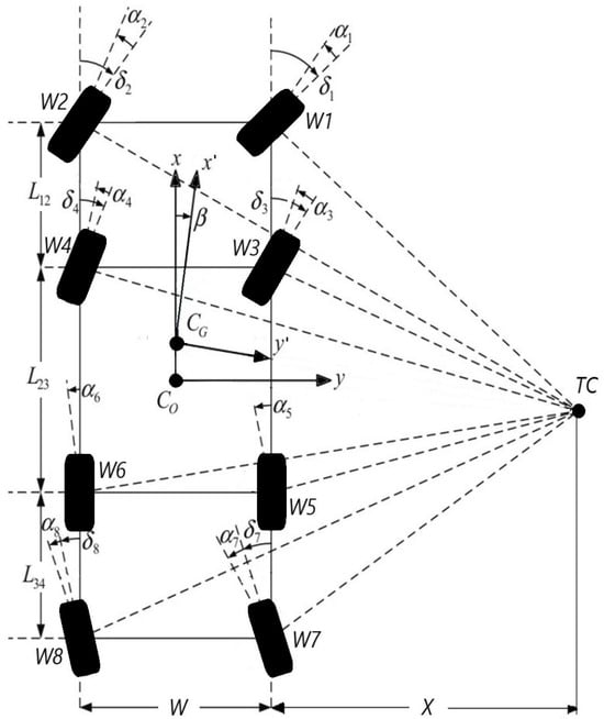
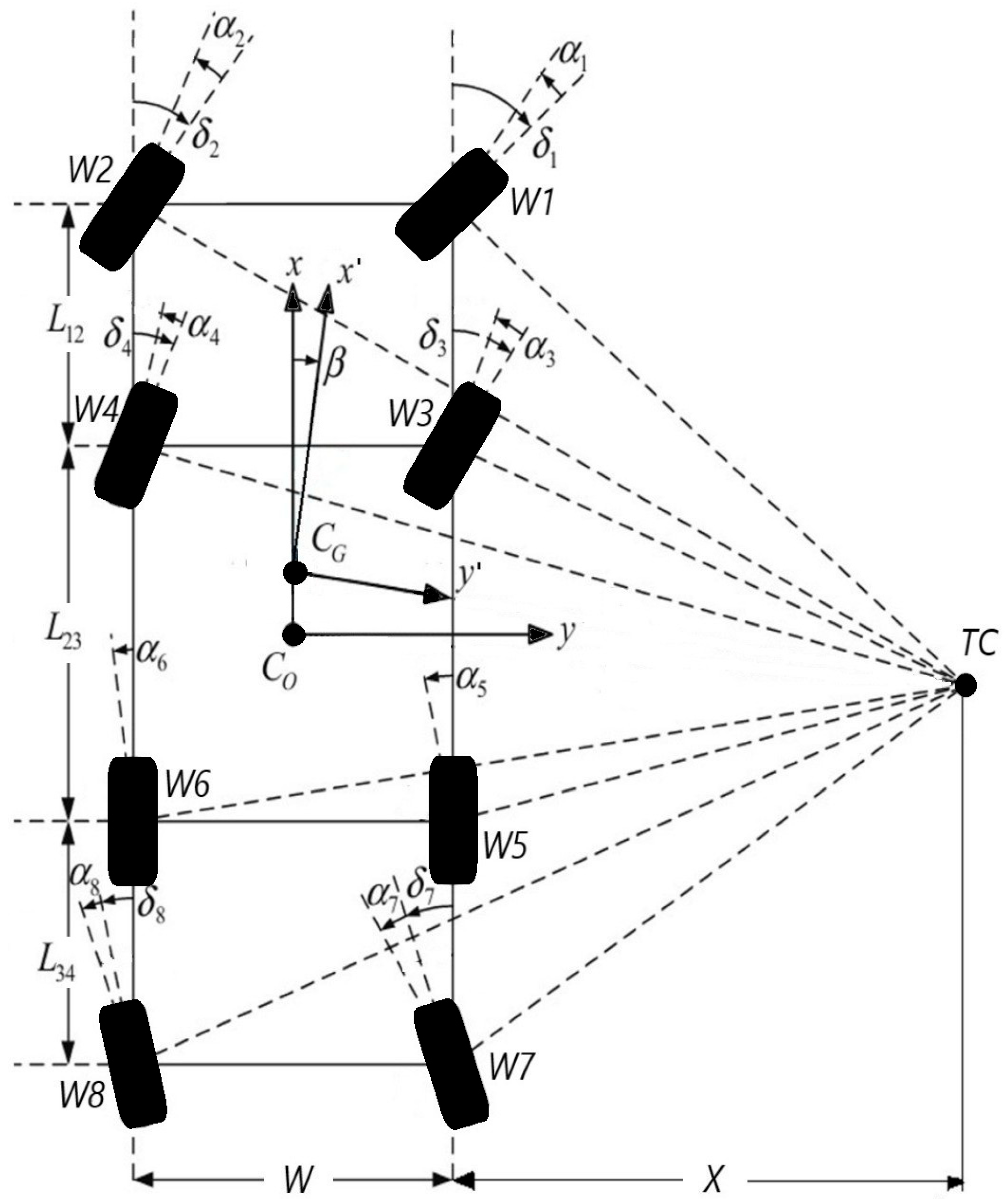
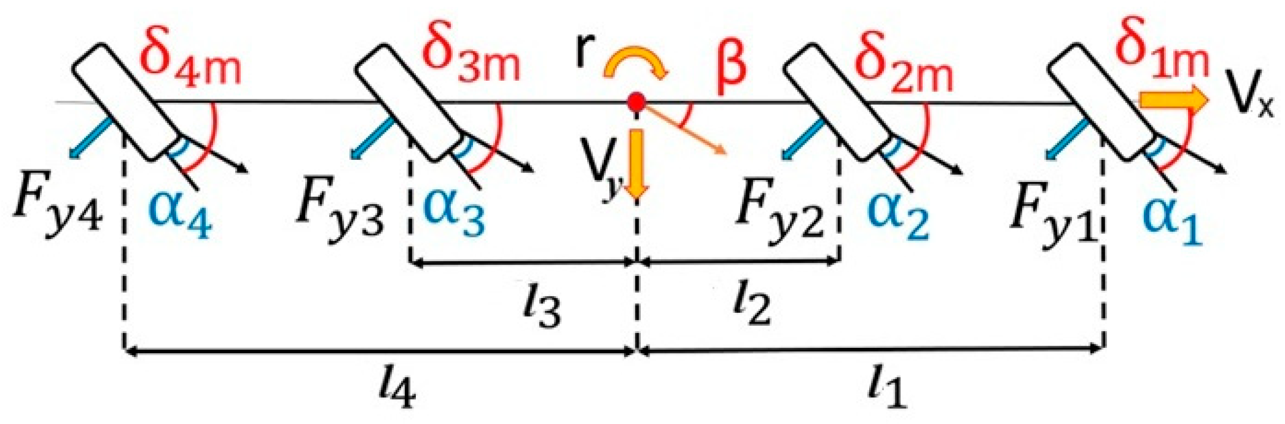
As far as a four-axle vehicle model is concerned, the motion model is as shown as Figure 2. is the center of vehicle body, is the center of gravity (CG) of the vehicle, and W is the tack width, which is the distance between left and right wheels. When the vehicle turns, the position of the instantaneous center TC will be located at the intersection point of the normal lines of the eight wheels. After setting the steering angles of the eight wheels, the position of TC can be found by the model constructed in Figure 2 with the geometrical method.
Figure 2.
Four-axle vehicle motion model. L12, L23, L34 are the longitudinal distances between axles, W is the track width of vehicle, is the steering angle of each tire, is the slip angle of each tire, is the turning radius of COG, and is the turning radius of body geometric center; β = Vy/Vx [27].
When the position of the instantaneous center is calculated, other motion parameters can be calculated, such as the turning radius of (Equation (1)), turning radius of body center RO (Equation (2)), side slip angle α, and so on.
where and are the x, y components of the instantaneous center, and and are x, y components of CG.
The proper relationship between the steer angle of the inside wheel and that of the outside wheel should satisfy the well-known Ackerman formula:
Formally, the slip angle is defined as follows (Figure 2):
where is the slip angle of i-th tire, is the steering angle of the i-th tire (including steer input and slip angle), is the lateral velocity, and is the longitudinal velocity.
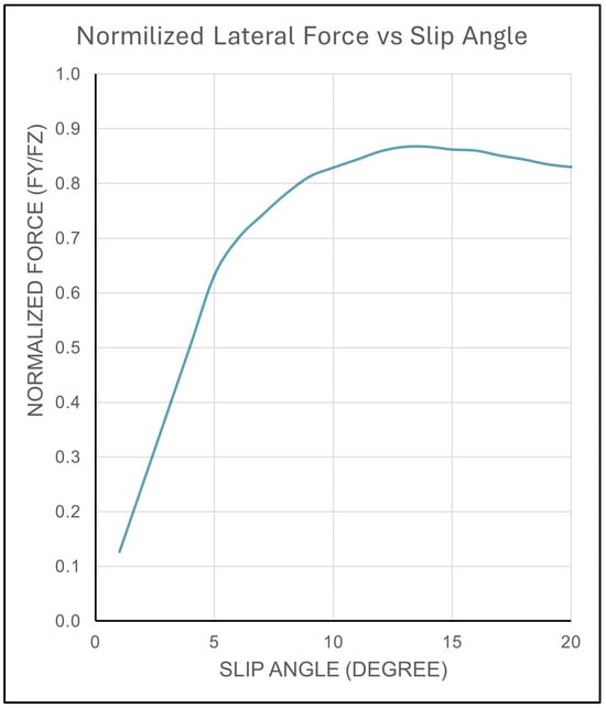
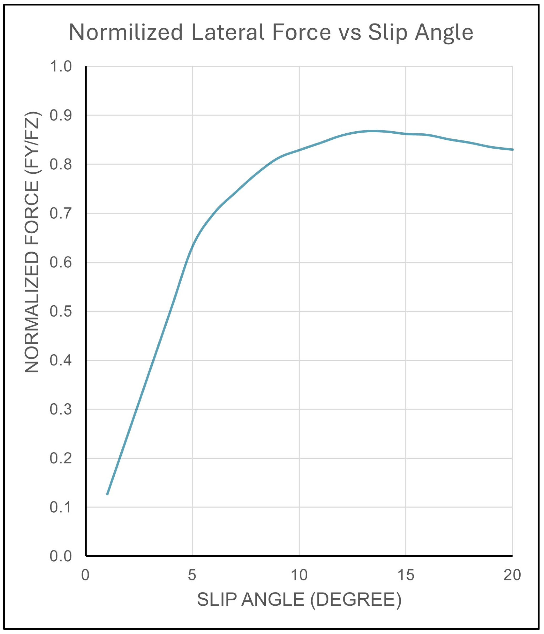
Tire characteristics, vehicle speed, steering angle, load distribution, and road conditions are some of the important variables affecting slip angle. The magnitude of the steering angle directly influences the slip angle, as larger steering inputs typically result in larger slip angles. Wet, icy, or uneven surfaces can change the friction between the tires and the road surface, which can have a substantial effect on the slip angle [25,26,28]. The surface adhesion is a significant component that greatly affects the calculation of the lateral force. For medium cars, tire lateral force is linearly changing up to 5–6 degrees [29]. The lateral force against slip angle is similar for truck tires on dry concrete surface for 88 kph forward speed is shown in Figure 3 [27,30,31]. The linear relationship between the lateral force and the slip angle is applicable for slip angles up to about 6–7 degrees. The linear relationship will no longer yield a reliable approximation for increasing slip angles.
Figure 3.
Lateral force normalized with vertical load slip angle change of truck tire for 88 kph speed over dry concrete surface [27,30,31].
1.2. Bicycle Model
The bicycle model is a simplified representation of a vehicle’s motion that helps in understanding and predicting its behavior during steering maneuvers. Despite its simplicity, this model is particularly useful for analyzing the fundamental aspects of vehicle dynamics and control strategies in both research and practical applications. This model focuses on the vehicle’s lateral and yaw dynamics, capturing key behavior during turning and stability control.
In mathematical formulation, the vehicle is assumed to have a rigid body. Additionally, the wheels are assumed to be massless, and only the forces acting on the vehicle body are considered. Tire forces are linearized for small slip angles, making the model applicable primarily for low to moderate speed scenarios. The bicycle model uses a coordinate system with the origin at the vehicle’s center of gravity. The x-axis points forward, and the y-axis points laterally to the left. The bicycle model ignores aspects like the load transfer, suspension effects, and non-linear tire performance at high slip angles, which oversimplifies the true dynamics of multi-axle vehicles.
1.3. DOE and the Taguchi Method
The Taguchi Method is developed for designing experiments to investigate how different parameters affect the mean and variance of a system’s parameters on responses. The experimental design proposed by Taguchi involves using orthogonal arrays. Instead of having to test all possible combinations like the factorial design, the Taguchi Method tests pairs of combinations, which allows the collection of necessary data to determine the factors that most affect the response with minimum experiments [32]. The primary objective of the Taguchi robust design is to ensure that systems and products perform reliably regardless of uncontrollable external factors, thereby minimizing the impact of variations that cannot be controlled or eliminated [33].
The quality loss function, introduced by Taguchi, quantifies economic loss due to deviations from target performance using the following formula [32,33,34]:
where L is the loss function, k is a constant, y is the actual value, and m is the target value. This approach shifts the focus from simple compliance to minimizing deviation from the target. OAs are central to the Taguchi Method, enabling the study of multiple factors simultaneously with a reduced number of experiments, allowing for efficient data collection and analysis even in complex systems.
Implementing the Taguchi Method involves a series of structured steps to ensure effective optimization: first, clearly identifying the problem, setting the objectives, and determining the quality characteristic to be optimized (response variable) [33]; next, identifying the factors affecting this quality characteristic and defining the levels (values) for each factor to ensure that all relevant variables are considered; then, selecting an appropriate orthogonal array that fits the number of factors and levels, based on the desired resolution and the number of interactions to be studied. Conducting experiments according to the OA and collecting accurate and reliable data for the response variable are the following steps. The process continues with analyzing the results by calculating the S/N ratios for each experiment and using analysis of variance (ANOVA) to determine the significance of factors, thereby identifying the optimal levels for each factor. Finally, predicting the performance at these optimal settings and conducting confirmation experiments to verify the predicted performance ensure the reliability of the optimization [33].
To determine the effect of each variable on the response, the signal-to-noise ratio, or the S/N number, needs to be calculated for each conducted experiment. For the case of minimizing the performance, the following formula for the S/N ratio should be calculated:
For the case maximizing the performance characteristics, the ratio should be calculated with the following:
where is the experimental number, is the trial number, and is the number of trials for experiment .
One of its primary advantages is the cost-effectiveness, as it reduces the number of experiments needed, thereby saving considerable time and resources. Additionally, it provides a systematic approach to problem-solving and optimization and focuses on creating products and processes that are insensitive to variations, enhancing robustness. However, the Taguchi Method also has some limitations that necessitate careful application. It operates on several simplistic assumptions, such as assuming that factors are independent, which may not always be the case in real-world scenarios. Furthermore, it primarily focuses on linear models, potentially overlooking complex interactions that could be critical to the optimization process [34]. Despite these limitations, when complemented with other methods, the Taguchi Method can significantly contribute to achieving excellence in product design and manufacturing processes.
2. Materials and Methods
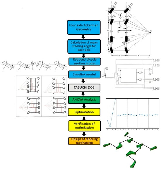
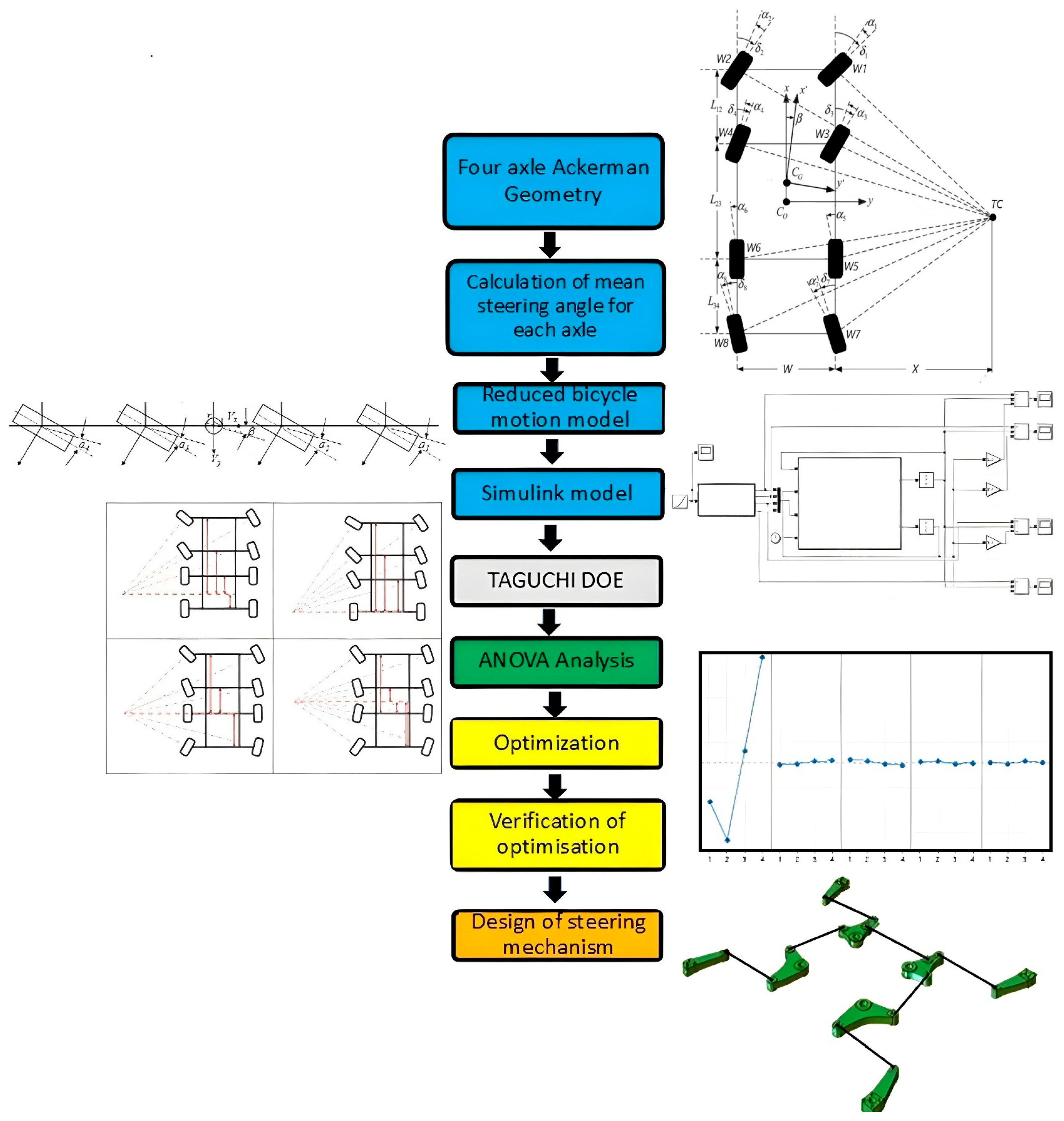
In this study, an optimized steering strategy is developed to satisfy both low turning radius at low speeds and steering stability at high speeds for an 8 × 8 vehicle. The methodology used in this study is schematically summarized with Figure 4.
Figure 4.
Methodology used for optimization and linkage design study [27].
This study started with mathematical modeling and simulation of vehicle motion, which provides the ability to analyze complex systems quickly and accurately and test and optimize various scenarios.
In the optimization part, the Taguchi Method is employed, which saves time and simulation cost by reducing the number of experiments. It is effective in optimizing parameters when the interaction between variables is limited and increasing the robustness of the system against external factors. The method is effective in linear models and may ignore complex interactions. In final part of the study, a four-bar mechanism is developed and checked with multi-body dynamics simulations.
2.1. Design Objectives
In the benchmark research on 8 × 8 vehicles, it is noticed that one of the most important design criteria, as mentioned before, is to achieve a minimum turning radius. In this study, an 8 m turning radius is taken as the design objective, which is a reasonably challenging target. While achieving the turning radius target, the steering angle of the wheels was limited to 40 degrees. Larger steering angles may cause a conflict in terms of kinematics or packaging. The preliminary calculation consists of steering angles for every DOE scenario and a mean steering angle for each axle.
Valid data is very important for realistic motion simulations. However, detailed and accurate data is difficult to obtain, especially for four-axle vehicles. Therefore, a detailed literature survey has been conducted, and the base vehicle parameters used in the motion model are summarized at Table 1. The moment of inertia is taken from the author’s previous works on 8 × 8 vehicles’ structural analysis using the finite element method, but similar data is also available in the literature [16].
Table 1.
Vehicle properties used for bicycle model.
The cornering stiffness for a medium car would be about 140–200 kN/rad [29]. After completing benchmark research for the 14R20 tires, in most studies, cornering stiffness is stated to vary between 150–300 kN/rad [35]. Due to weight distribution, front axle tires have higher cornering stiffness than the rear tires [16,29,35]. In the present study, tire stiffness C1 and C2 were chosen to be 200,000 N/rad for the first two axles (total shall be 400,000 N/rad for each axle in bicycle model), and the stiffness values of the other axles were calculated artificially by decreasing it 10%, thus C3 and C4 were taken as 180,000 N/rad. The longitudinal velocity used in simulations is 20 m/s. This means that the vehicle steering system designed for low-speed conditions achieves an 8 m turning radius and moves at an average highway speed on asphalt road with the same steering dynamics.
Generally, lane change is the most widely used maneuver for investigating stability analysis [7,9,16]. A half sinus wave was used as the steering input angle to represent a lane change maneuver. This simulates the vehicle making a 6-degrees (0.1 radians) turn and returning to the starting point within 5 s, and the maximum slip angle is calculated for each axle accordingly.
2.2. Mathematical Modeling
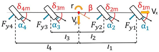
The multi-axle vehicle-bicycle motion model formulations for an 8 × 8 vehicle with all-wheel steering (AWS) are presented in Figure 5. The steering angles are the means of the left and right tire steering angles for each axle, which comply to Akerman’s principle for each configuration. In the example, for the first axle, is the mean of and shown in Figure 2. For a four-axle vehicle, the multi-axle bicycle motion model equations can be written using force and moment equilibrium as follows [9,16,25,26]:
where is the distance of the i-th axle to the center of gravity, and is the lateral force of the i-th axle.
Figure 5.
Schematic representation of bicycle model for the four-axle vehicles [9].
For small steering angles,
We can write the slip angle with the following equation:
For small steering input angles, the slip angle can be written as follows:
Wheel lateral force can be represented by the slip angle and the lateral force stiffness:
where is the cornering stiffness of tires of the i-th axle. Then,
and
For small steering input angles, ; therefore, we can simplify that:
After rearranging to leave and at the right side of the equation, the state space matrix will be achieved as follows:
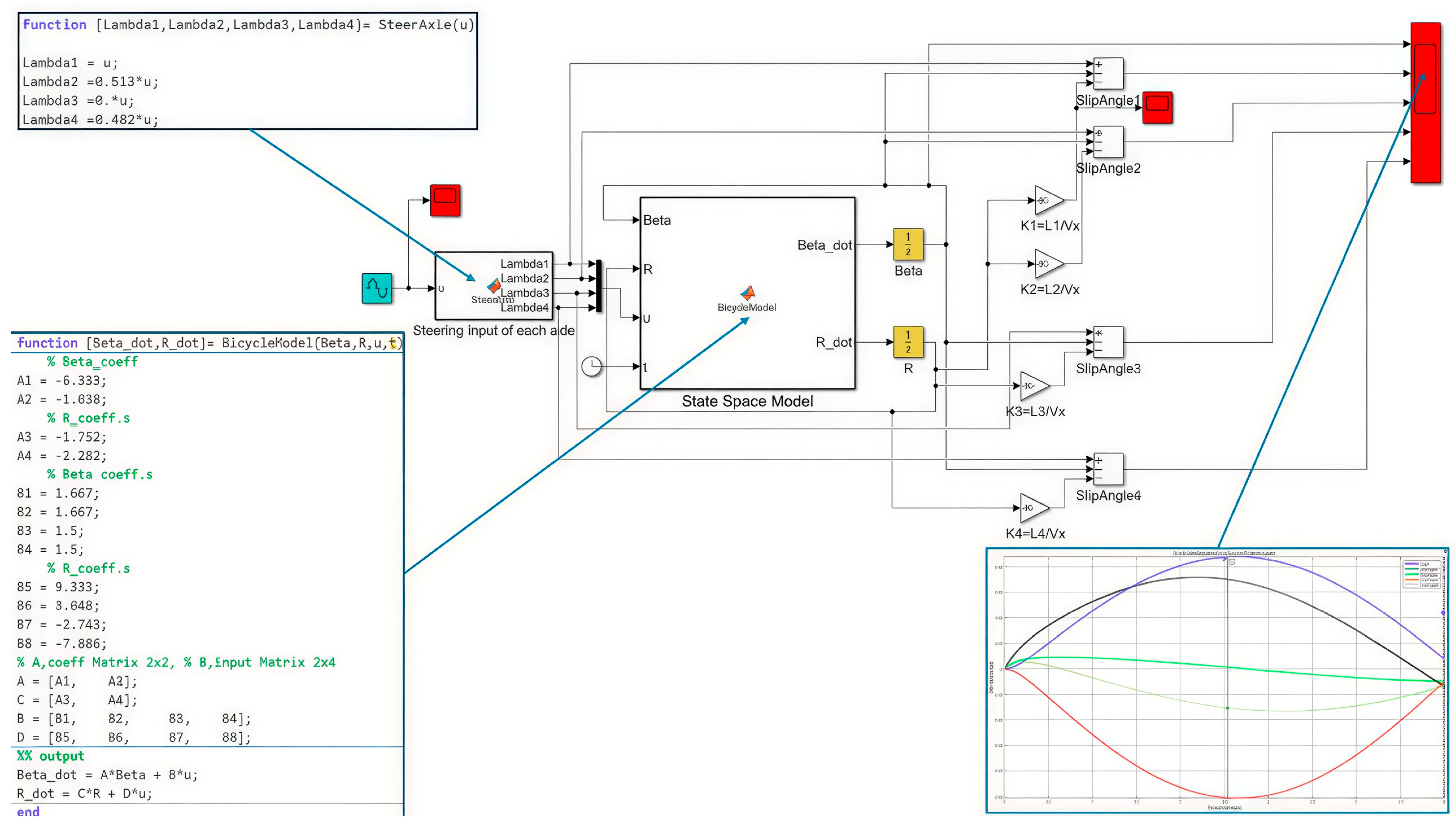
Equation (20), which is the result of the calculations and modeling, was remodeled for processing through MATLAB-Simulink software version 2023b. In order to simplify data input, Equation (20) is converted to the form shown with Equation (21).
The MATLAB/Simulink model is shown in Figure 6. The first axle steering input is given with a sinusoidal source 0.1 radians amplitude, 0.6282 frequency, and 5 s simulation time. The steer input data is distributed to other axles using a second block named “Steer Axle”. In a state space block, Equation (21) is converted to a function with outputs and . Outputs are integrated to calculate the slip angle using Equation (13). The scope block was integrated to read the desired output values, such as slip angles and the vehicle steer angle. The sample time of simulation is 1.0 × 10⁻⁴, and the “ode43” Runge-Kutta fourth order solver was chosen.
Figure 6.
Matlab/Simulink model.
2.3. Design of Experiments
A four-level DOE with five parameters is defined and L16 orthogonal array selected to establish experiment scenarios. A total of sixteen scenarios were defined for four different steering configurations and analyzed with Minitab software [34]. For each configuration, four different scenarios were created. The parameters defined for each scenario are shown in Table 2.
Table 2.
DOE scenarios and calculated axle steering angles for 8 m turning radius.
In this table, ““ represent the distance between the axle and the center of gravity of the vehicle in meters. Equation (3) was used to calculate the steering angles for each scenario, providing a turning radius of 8 m. Here, represents the average of the steering angles of the left and right wheels on the axle.
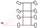
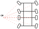
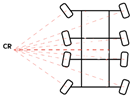
In Table 2, Configuration 1 represents the steering of the first two axles, Configuration 2 represents the steering of the first three axles, Configuration 3 represents the steering of the first, second, and fourth axles, and Configuration 4 represents the steering of all the axles. Secondly, steering angles for each configuration and axle distances were calculated and mean steering angles tabulated in Table 2 for bicycle motion model. Parameter represents the average of the steering angles of the inner and outer wheels of the i-th axle.
3. Results
3.1. Stability Analysis
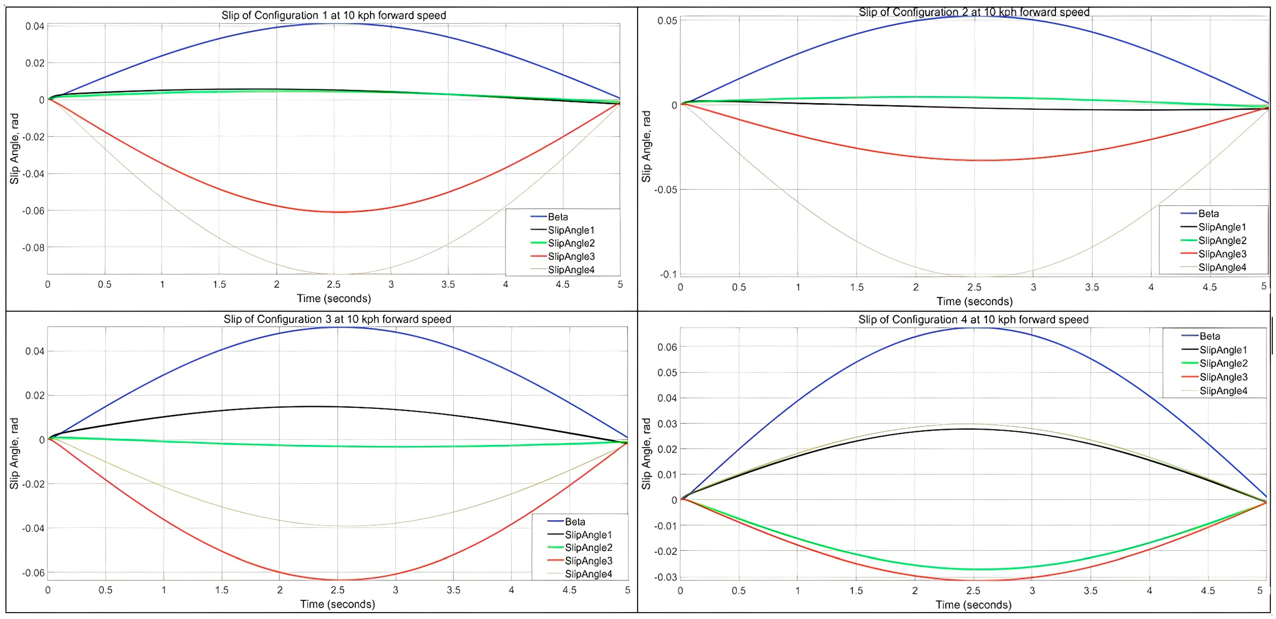
To understand the steering performance and stability of the simulated vehicle, as a preliminary study, slip angles were checked for each configuration at 10 kph with a half sinusoidal steering input with an amplitude of 6 degrees for the first axle. The steering input of other axles was activated according to the steering ratios given in Table 2. With a half sinusoidal input, the vehicle first turns right and then left with the same amplitude and rate to ensure that the final steering position of the vehicle is a neutral position when the best performance happens. Slip angles for each axle and vehicle turning angle are graphed with the same axle distances for 10 kph forward speed. As shown in Figure 7, each steering configuration shows various slip angles and steering angles. It is evident that a vehicle reaching a higher steering angle and showing low slip angles has the best turning performance.
Figure 7.
Slip angle and vehicle turning angle of four different steering configurations at 10 kph speed and 0.1 radians sinusoidal input.
The results of steering configuration 1 show that since the first two axles are steered, the slip angle is quite low at these axles, but when the solid axles are taken into consideration, there is a significant slip and resistance to the turning maneuver. For the ideal case, the vehicle turning angle should be close to the first axle steering input. Of course, due to axle distance and orientation, we do not expect full compatibility with Ackerman. Therefore, it can be concluded that the turning performance is low for Configuration 1. In the second configuration, the first three axles were steered, and therefore the slip angles are low at these axles and higher at the fourth axle, which is a solid axle. Vehicle steer angle is higher than configuration 1, which means better turning performance is achieved. The solid axle slip angle is close to the first axle steering input amplitude. As easily noticed, the best turning performance is achieved when all axles are steered (Configuration 4). The first two and last two axles show similar slip angles, but in opposite directions. The vehicle turning angle is significantly better than the other configurations but still could not reach the theoretical value due to axle orientation and limitation due to package considerations (max. 40 degrees allowed for the first axle). When only turning performance is taken into consideration, the configuration order from high to low is 3–4–2–1.
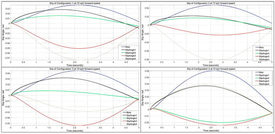
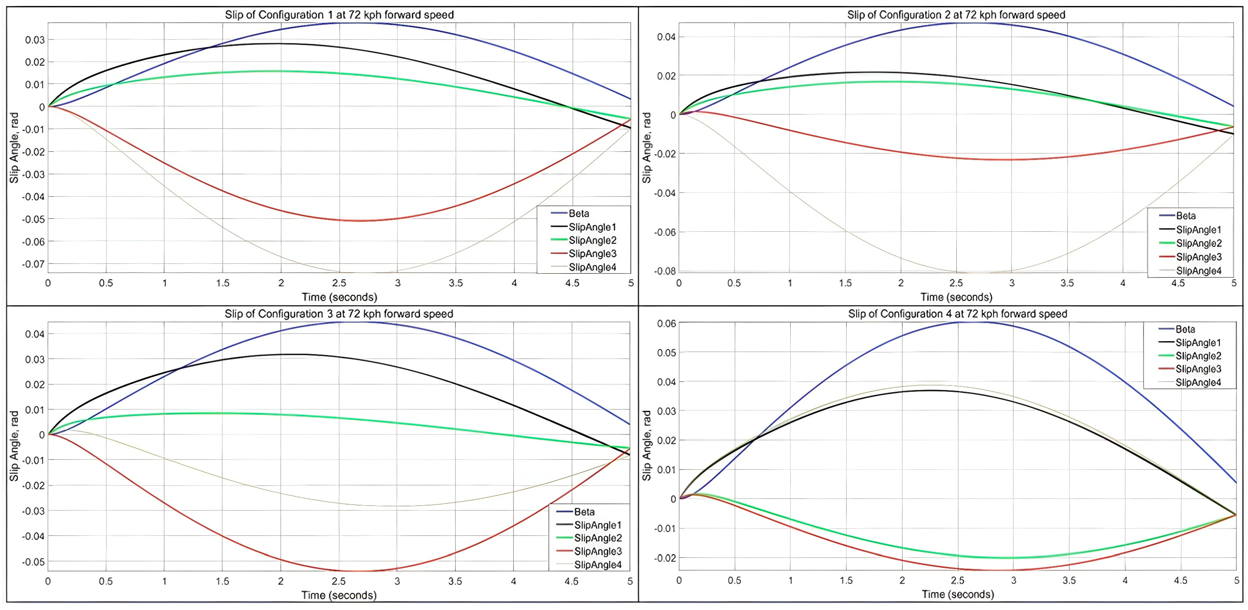
If a similar study is performed for 72 kph forward speed without changing the parameters, it will be clearly seen that stability will deteriorate with increasing low speed turning performance. At first glance of Figure 8, vehicle steering angle is not returning to the neutral position while the maneuver is completed. The highest difference can be shown in Configuration 4, which is 0.006 radians. The second configuration has 0.003 radians, and the best is Configuration 1, which is 0.002 radians.
Figure 8.
Slip angle and vehicle turning angle of four different steering configurations at 72 kph speed and 0.1 radians sinusoidal input.
In order to design a high-performing vehicle from a stability point of view, the steering angle deviation from the neutral position and total slip angle should be minimized. Therefore, investigation proceeds using two parameters. The first response is the total deviation of the steering angle, and the second parameter is the sum of the absolute magnitude of maximum slip angles.
3.2. Taguchi Optimization Results
With the help of Minitab software [35], optimization studies were carried out according to the Taguchi Method. Here, L1, L2, L3, and L4 represent the distance of the axles from the center of gravity in different scenarios. Parameters “L1” and “L4” vary between 2300 and 2450 mm, and “L2” and “L3” vary between 800 and 950 mm.
In Table 3, state space parameters for each DOE set are shown. Based on the calculated parameter set, the MATLAB/Simulink model was run, and slip angle for each axle, maximum turning angle of vehicle , and vehicle turning angle delay are tabulated in Table 4.
Table 3.
State space parameter defined in Equation (21) for each DOE scenario.
Table 4.
Slip simulation results for DOE scenarios.
The DOE results are tabulated in Table 4. Columns 2–5 are the calculated slip angles based on Equation (13) for each axle. Column 6 represents the mean of the slip angles for all axles. The seventh column is the maximum turning angle of vehicle , and column eight is the vehicle turning angle delay between the starting and ending times of maneuver .
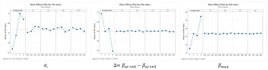
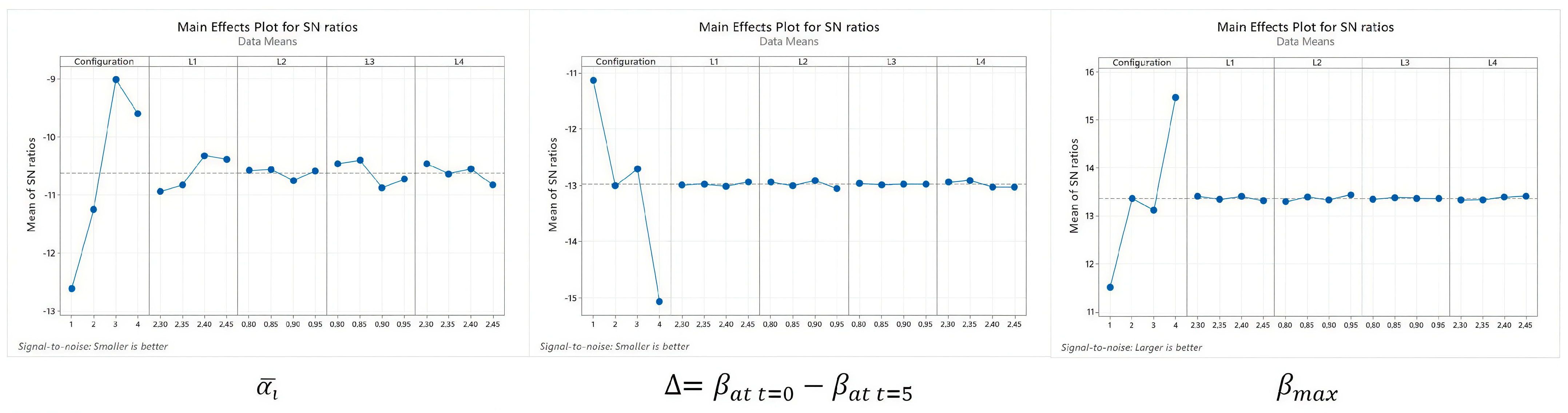
Figure 9 shows the main effects plot for slip angle, steer angle, and steer delay separately. The minimum mean slip angle is seen for Configurations 3 and 4, but on the contrary, the minimum delay occurs for Configuration 1. As a preliminary outcome, minimum slip and max stability could not be achieved with the same steering configuration. In fact, this is a common understanding that all vehicle manufacturers are aware of. In most 8 × 8 military vehicles, in order to achieve the minimum turning radius, all-wheel steering is applied, but most of them have a deactivating control for the third and fourth axles during highway driving conditions. The basic conclusion from the DOE study is in line with this state-of-the-art solution.
Figure 9.
Main effects plot for slip, delay in vehicle steering angle at t = 5 s, maximum vehicle steering angle using sign-to-noise ratio in vertical axis. Affecting parameters are Configuration, L1, L2, L3, and L4 are at given in horizontal axis.
As stated in Table 5, analysis of variance (ANOVA) results show that the most significant parameter for slip angle, angle delay, and vehicle steering angle is the steering configuration. The p-value is less than 0.05 for each response, showing that the significance of configuration is high. The other parameter such as L1–L4 on the response is quite low. Another important feature of ANOVA analysis is the residuals calculated for each event. When the calculated sum of the square of the residuals increases, the regression equation represents the events more accurately.
Table 5.
ANOVA analysis and linear regression optimization results.
On the other hand, increased number parameters can also increase the R-sq value; therefore, R-sq adjusted is more conveniently used to understand the effectiveness of regression equation. When the R-sq and R-sq adjusted values are close to each other and are high (around 80%), the number of parameters is sufficient. When R-sq predicted is also high, it proves that the regression model can predict new values out of DOE events, and there is not any lack of a missed variable.
Minitab optimizer tool is used to find best values within the range defined for each parameter separately. For the mean slip, the minimum value is 2.49 × 10⁻² radians, which is achieved in the third configuration. The minimum angular delay during the sinusoidal maneuver is found to be 3.54 × 10⁻³ radians in Configuration 1.
For the mean slip angle, R-sq and R-sq adjusted values have a significant difference; therefore, it can be concluded that some parameters have not been taken into account as variables, such as track width, cornering stiffness, or adding each wheel angle. The difference between R-sq and R-sq adjusted is less for delay and vehicle steer angle.
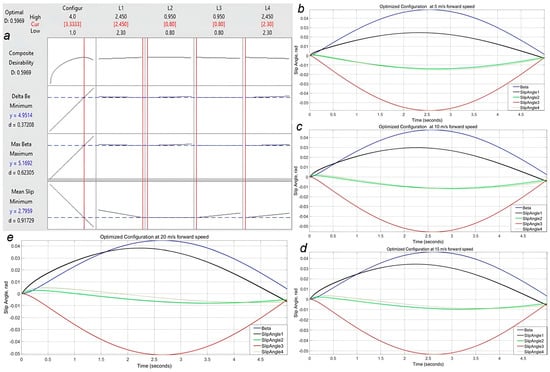
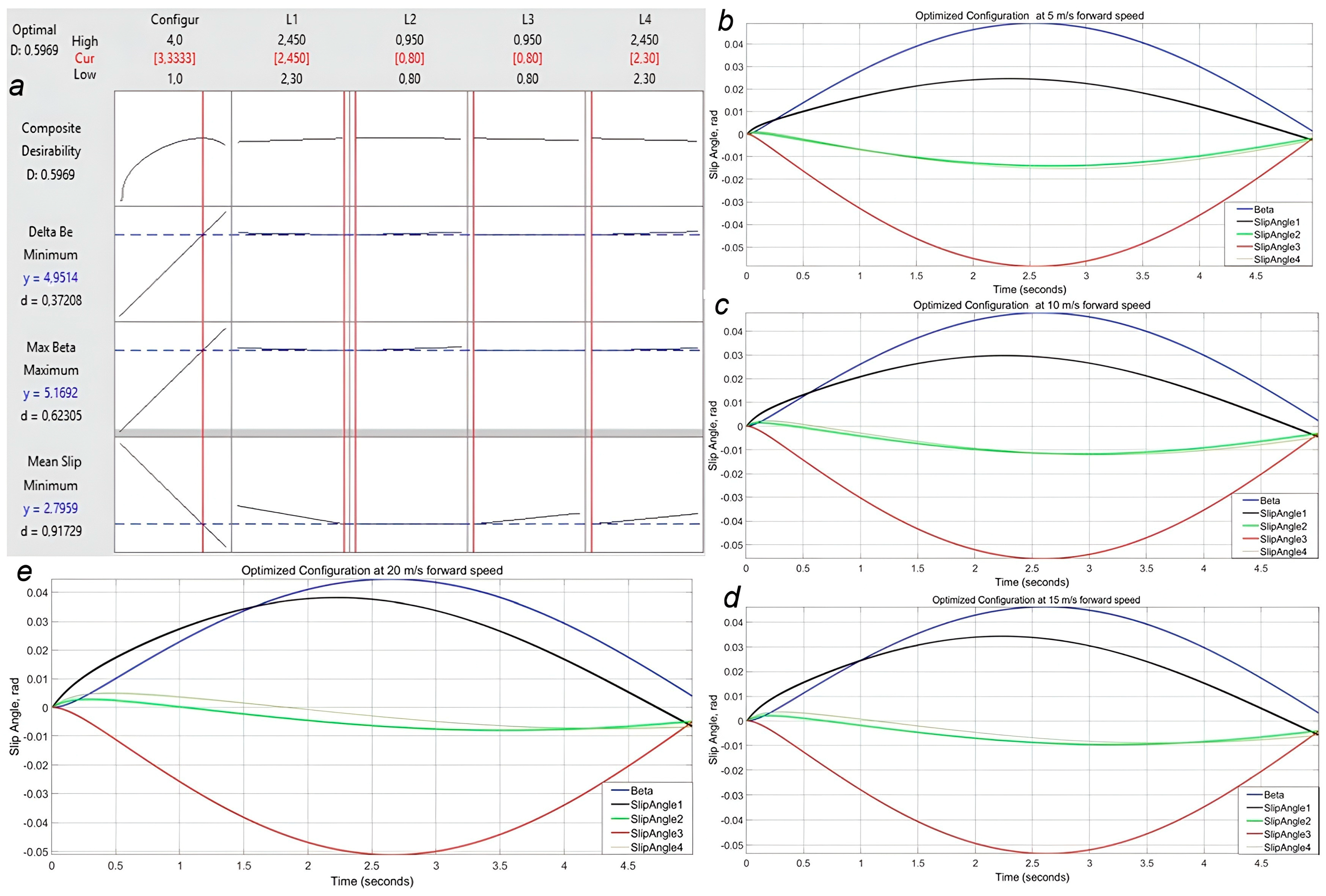
Additionally, the Minitab optimizer (version 19) is used to find whether there is a solution in which all responses could be optimized. The results are shown in Figure 10a. When compared with Table 5, as expected, there is not a single configuration wherein all responses are optimized. The composite desirability value (D = 0.6) is quite low, which means the proposed solution is not fully representative. Also, desirability values for and are low, which means the optimizer results are not very dependable.
Figure 10.
Composite optimization, mean slip minimum, deviation from neutral steering angle minimum, vehicle steering angle maximum. (a) Minitab optimizer results (b–e) MATLAB/Simulink result with optimized variable at 5-10-15-20 m/s forward speeds.
Minitab optimizer results conclude that the steering configuration that satisfies all three responses is close to Configuration 3, with L1 = 2.45 m, L2 = L3 = 0.8 m, and L4 = 2.3 m. Figure 10b–e shows the performance of the vehicle with the calculated parameters for speeds 5–20 m/s. For the mean slip, the minimum value is 2.54 × 10⁻² radians, and the minimum angular delay during the sinusoidal maneuver is found to be 4.19 × 10⁻³ radians.
4. Implementation to Linkage Design
Although Configuration 3 has significantly lower slip angles at low speeds, at elevated speeds, Configuration 1 shows the better stability performance. In this study, since we could not find a single solution to our design requirements with high confidence, the high-speed handling capabilities and the turning radius of the vehicle were optimized by selecting the third configuration, in which axles 1, 2, and 4 are steerable. Usually, in order to keep handling performance safe without losing maneuverability at lower speeds, the low-speed and high-speed steering strategies differ in a multi-axle vehicle. In this strategy, the vehicle is steered in all wheels for low vehicle longitudinal velocities, and when the longitudinal vehicle velocity is higher than a specific value (generally 30 kph), the rear axles (third and fourth) are kept fixed at nominal position, and the vehicle is steered only by the front four wheels.
For the third configuration, axle 3 is kept fixed, and other wheels are steerable. The steering angles are calculated using Equation (3) for the 8 m turning radius as follows.
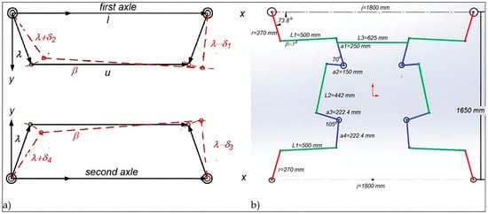
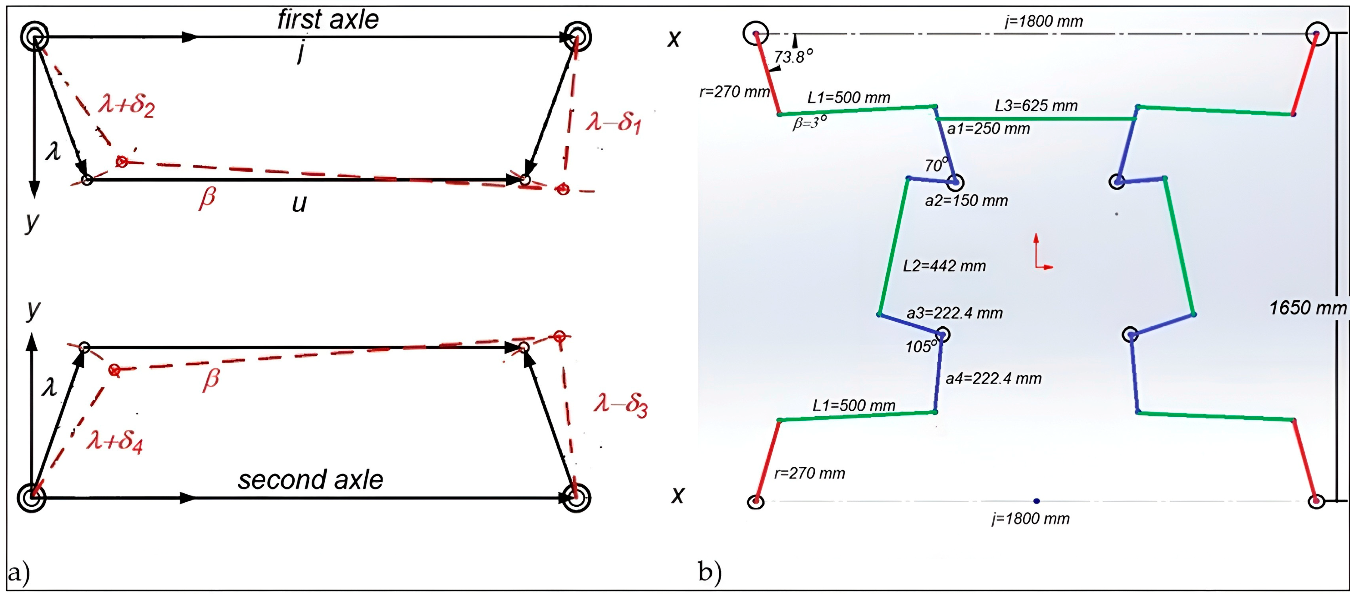
The Ackermann steering mechanism or trapezoidal steering mechanism, as shown in Figure 11a, is a symmetric four-bar linkage with equal lengths of the input link and the output link, , while the length of the connecting link is smaller or larger than the length of the fixed link . If is smaller than , it is arranged as a trailing Ackermann steering mechanism; otherwise, if is larger than , it is arranged as a leading Ackermann steering mechanism [12]. In Figure 11a, solid lines represent the trapezoidal steering mechanism during straight travel, while red dotted lines show it during a left turn.
Figure 11.
(a) Four-bar steering mechanism and (b) its application to the first two axles.
The first two-axle linkage design is developed using a trapezoidal four-bar mechanism, in which ratio is generally taken between 0.10 and 0.15 [36]. Since the optimized steering angle value is close to 30 degrees, the ratio is taken as 0.15. Using Figure 10b, the equation is derived by simply calculating total travel in x and y directions when making the maximum turn. The value is calculated using Equation (22) [37,38,39]:
where (19.48°) is the first axle outer wheel angle, (25.51°) is the inner wheel angle, λ is the drag link angle at neutral position, is the drag link length, and is the distance between kingpins in x direction.
In this equation, since the values of and are previously calculated, they are substituted in, and the ratio of r and j is determined to be 0.15. The value of j, which corresponds to the distance between the two kingpins on the front axle, is determined to be 1800 mm. To achieve the desired angle values, attempts were made by assigning r/j ratios of 0.13, 0.14, 0.15, and 0.16 and using angles in different orientations. By setting to 3 degrees and using an r/j ratio of 0.15, the closest value to the target was obtained. It was observed that the most significant factor in altering the value was the adjustment of the angle. The best λ and r values for the developed configuration are 16.2° and 270 mm, respectively. The L1 link makes a negative 3° angle and a length of 500 mm. Pitman arm dimension a1 is equal to 250 mm, and a2 is 150 mm. In order to achieve the steering ratio between the first and second axle idler arm, the b1 and b2 dimensions are set to 222.4 mm. L2 is 442 mm, and the longitudinal distance between the first and second axle kingpin points is 1650 mm. All steering hardpoints are shown in Figure 11b.
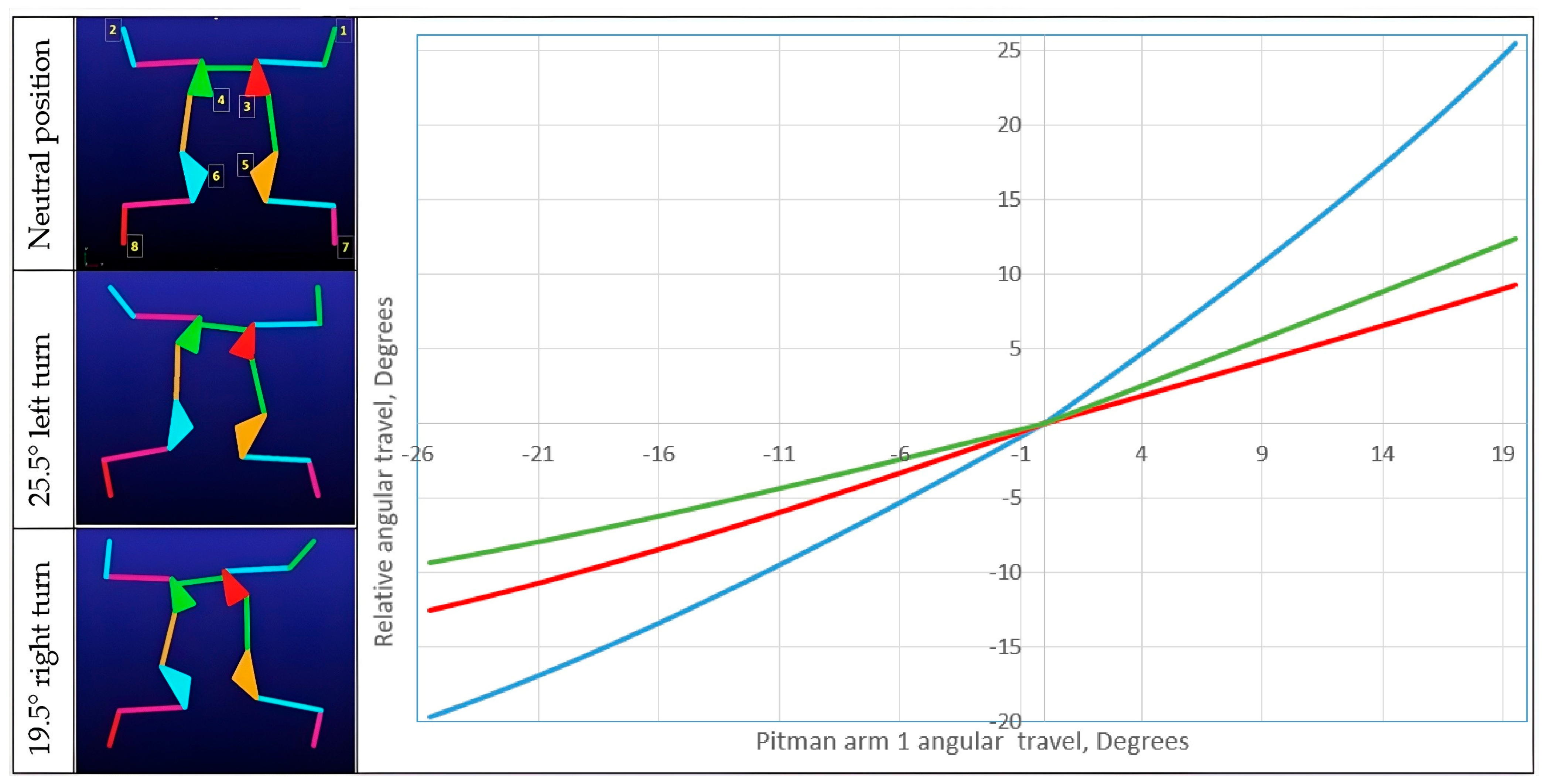
In order to verify the established geometry, the kinematics model was implemented in ADAMS/View (version 2025) multibody dynamics software. The model and resultant angle travel for the uppermost left and right turns are shown in Figure 12. The deviation from theoretical values is below 0.8%.
Figure 12.
ADAMS/View simulation results. The horizontal axis shows the , the blue line is , the green line is and the red line is
5. Discussions
During this study, various approaches and tools are used to develop a steering system that performs well both in cornering at low speeds and lane changes at high speeds. In order to achieve these objectives, a bicycle motion model is implemented in MATLAB/Simulink (version 2023b) to predict the slip angle for various design settings. To achieve reasonable and accurate outcomes, the model is run within a linear range of tire lateral stiffness. A linear regression relationship was developed using L16 Taguchi orthogonal array, which includes five parameters and four levels. Responses are analyzed using the ANOVA method, and the optimum solution is generated and discussed deeply. The R-sq values found around 0.8 indicate that the parameters could be increased to have a higher confidence level, such as track width, cornering stiffness, or adding each wheel angle separately and using a full car model including suspension effects.
Since our first target is to show the general tendency of steering configuration, the existing number of parameters and the application of the bicycle model are sufficient. First, mean slip, vehicle steer angle, and delay in steering maneuvering are investigated to understand the effects of the parameters. This initial inspection helped to understand the characteristics and behavior of the responses and definitively showed that minimizing turning radius and increasing the stability of the vehicle are in conflict with each other. The minimum slip occurs with Configuration 3, the maximum vehicle steer angle occurs with Configuration 4, and the minimum delay occurs with Configuration 1.
Slip angle calculations show that Configuration 3 gives the lowest slip angle (Figure 8, Table 5). When the vehicle is designed for high maneuverability in off-road conditions and changes lanes at a speed of 72 kph on an asphalt road, significantly increasing slip occurs. Additionally, the vehicle will not return to its neutral position even if the steer angle reaches zero. This reduces driving safety, damages linearity in steering control, and leads to tire wear.
Minitab optimizer results conclude that the steering configuration that satisfies all three responses is close to Configuration 3, with L1 = 2.45 m, L2 = L3 = 0.8 m, and L4 = 2.3 m, which steer the first, second, and fourth axles, respectively. The developed solution is used in the design of a four-bar Ackerman mechanism of the first two axles without a linkage added to the third axle. The mechanism is modeled using ADAMS/View (version 2025) and checked virtually to confirm whether the wheels’ travel during left and right turns are in line with the Ackerman geometry.
6. Conclusions
Although the applied methodology proposes an optimized solution to low turning radius and stability at high speeds, a reliable 8 × 8 vehicle steering system depends entirely on the way the vehicle is used. Configurations 4 and 3 are preferable in cases where high maneuverability is desired, and Configuration 1 works well in cases where a low steer angle delay is expected. In such a case, vehicles that can simply switch between configurations by locking the rear two axles when exceeding a certain speed will provide positive results in both types of use. The state-of-the-art application to military vehicle steering systems is similar [19,21]. It is not surprising that the recent studies related to multi-axle vehicles are focused on control strategies [40,41,42]. However, this increases the cost of production and maintenance. The proposed solution with this study can be a worthwhile and cost-effective answer to the mentioned conflict.
Author Contributions
Conceptualization, N.K.; methodology, N.K.; software, M.Ç.; validation, N.K. and M.Ç.; writing—original draft preparation, N.K.; writing—review and editing, N.K. and M.Ç. All authors have read and agreed to the published version of the manuscript.
Funding
This research received no external funding.
Data Availability Statement
The data presented in this study are available on request from the corresponding author.
DURC Statement
Current research is limited to the research on steering dynamics for multi-axles vehicles, which is beneficial for increasing tire slip performance of vehicles to increase stability and driving safety in automotive engineering that does not pose a threat to public health or national security. Authors acknowledge the dual use potential of the research involving military and civil vehicles and confirm that all necessary precautions have been taken to prevent potential misuse. As an ethical responsibility, authors strictly adhere to relevant national and international laws about DURC. Authors advocate for responsible deployment, ethical considerations, regulatory compliance, and transparent reporting to mitigate misuse risks and foster beneficial outcomes.
Conflicts of Interest
The authors declare no conflicts of interest.
References
- Barone, M.G. High Mobility Tactical and Logistic Trucks: A European Global Overview. Mil. Technol. 2024, 3, 20–26. [Google Scholar]
- Barone, M.G. The 8 × 8 Phenomenon: Mobility, Protection, Firepower. Mil. Technol. 2020, 6, 20–23. [Google Scholar]
- Annati, M. Wheel of Fortune: Armored Vehicle Evolution. Mil. Technol. 2020, 6, 6–11. [Google Scholar]
- Giurgiu, T.; Virca, I.; Grigoras, C.; Nastasescu, V. Trends in Development of Military Vehicles Capabilities Based on Advanced Technologies. Int. Conf. Knowl.-Based Organ. 2023, 24, 15–22. [Google Scholar] [CrossRef] [Scilit]
- Zakaria, M.S.M.; Singh, A.S.P.; Aras, M.S.M. Integrated Chassis Control for Multi-Axle Vehicles: A Comprehensive Review. Int. J. Automot. Mech. Eng. 2024, 21, 11663–11681. [Google Scholar] [CrossRef] [Scilit]
- An, S.J.; Yi, K.; Jung, G.; Lee, K.I.; Kim, Y.W. Desired yaw rate and steering control method during cornering for a six wheeled vehicle. Int. J. Automot. Technol. 2008, 9, 173–181. [Google Scholar] [CrossRef] [Scilit]
- Zhang, Y.; Woo, A.; Fidan, B.; Khajepour, A. Adaptive yaw control of three-axle road vehicles based on mass, yaw inertia and CG position identification. In Proceedings of the Canadian Society for Mechanical Engineering International Congress 2018, Toronto, On, Canada, 27–30 May 2018; pp. 1–6. [Google Scholar] [CrossRef] [Scilit]
- Pereira, C.L.; Neto, R.T.C. Trajectory Control of a 6 × 6 Vehicle for Driver Assistance. In Proceedings of the Joint XLVI Ibero-Latin American Congress on Computational Methods in Engineering, Vitória, Brazil, 24–27 November 2025. [Google Scholar]
- Ahmed, M.; El-Gindy, M.; Lang, H. Path Following Enhancement of an 8 × 8 Combat Vehicle using Active Rear Axles Steering Strategies. Proc. Inst. Mech. Eng. Part K J. Multi-Body Dyn. 2021, 235, 539–552. [Google Scholar] [CrossRef] [Scilit]
- Bao, Y.; Du, C.; Wu, D.; Liu, H.; Liu, W.; Li, J. Coordinated Slip Control of Multi-Axle Distributed Drive Vehicle Based on HLQR. Mathematics 2023, 11, 1964. [Google Scholar] [CrossRef] [Scilit]
- Chen, P.A.; Chung, Y.J.; Chung, T.T.; Liu, T. Analysis of Steering Geometry and Design of Steering Mechanism for Four Axle Vehicles. In 2nd International Conference on Vehicle and Automotive Engineering; University of Miskolc: Miskolc, Hungary, 2018. [Google Scholar] [CrossRef] [Scilit]
- Kang, Y.W.; Pang, D.C.; Zeng, Y.C. Optimal Dimensional Synthesis of Ackermann Steering Mechanisms for Three-Axle, Six-Wheeled Vehicles. Appl. Sci. 2025, 15, 800. [Google Scholar] [CrossRef] [Scilit]
- Chung, Y.J.; Lin, T.; Liu, T. Analysis and Evaluation of 8 × 8 4-axle Vehicles with Assisted Steering System by Utilizing Mathematical and Computer Aided Design Models. In Proceedings of the 1st IEEE International Conference on Knowledge Innovation and Invention, Jeju Island, Republic of Korea, 23–27 July 2018. [Google Scholar] [CrossRef] [Scilit]
- Ozan, B. Steering System Optimization of a Heavy-Commercial Vehicle to Improve Straight Ahead Controllability Using Kinematics & Compliance Analysis. Master’s Thesis, Istanbul Technical University Mechanical Engineering, Istanbul, Türkiye, 2012. [Google Scholar]
- Saini, V.K.; Kumar, S.; Shakya, A.K.; Mishra, H. Design Methodology of Steering System for All-Terrain Vehicles. Int. Res. J. Eng. Technol. 2017, 4, 454–460. [Google Scholar]
- Bayar, K. Modeling of the Dynamics of Multi-Axle Steered Vehicles. Master’s Thesis, Middle East Technical University, Mechanical Engineering, Ankara, Türkiye, 2006. [Google Scholar]
- Bu, H.; Li, A.; Hunag, X.; Li, W.; Wang, J. Optimal Design of the Six Wheel Steering System with Multiple Steering Modes. Math. Probl. Eng. 2021. [Google Scholar] [CrossRef] [Scilit]
- Yazıcı, C.B.; Kutluay, E.; Unlusoy, Y.S. Steering optimization for multiaxle vehicles with multiaxle steering. J. Mech. Sci. Technol. 2021, 25, 3303–3311. [Google Scholar] [CrossRef] [Scilit]
- Otokar Arma 8x8. Available online: https://defense.otokar.com.tr/tekerlekli-zirhli-arac/8x8-zirhli-arac/arma-8x8-zirhli-arac (accessed on 12 August 2026).
- Avtoros Shaman 8x8. Available online: https://avtoros.com/en/shaman/?ysclid=msk62aijt396933455 (accessed on 12 August 2026).
- Airport Vehicles. Available online: https://www.rosenbauer.com/en-us/products/vehicles/arff-vehicles/panther (accessed on 12 August 2026).
- Mercedes Actross 8x8. Available online: https://www.autobild.de/artikel/bundeswehr-gepanzerter-actros-2793781.html (accessed on 12 August 2026).
- Stryker 8x8. Available online: https://www.oshkoshairport.com/arff-trucks/striker-8x8 (accessed on 12 August 2026).
- Patria 8x8. Available online: https://www.patriagroup.com/products-and-services/protected-mobility/wheeled-mobility/patria-amv-xp-number-1-in-the-battlefield (accessed on 12 August 2026).
- Wong, J.Y. Theory of Ground Vehicles, 3rd ed.; John Wiley and Sons: Hoboken, NJ, USA, 2001; pp. 31–33. ISBN 0471-35-4619. [Google Scholar]
- Gilespie, T.D. Fundamentals of Vehicle Dynamics; Society of Automotive Engineering: Warrendale, PA, USA, 1992; pp. 198–199. ISBN 1560911999. [Google Scholar]
- Cheng, H.; Hou, Z.; Liu, Z.; Li, J.; Zhang, J.; Zhao, Y.; Liu, X. Handling Stability Control for Multi-Axle Distributed Drive Vehicles Based on Model Predictive Control. Vehicles 2026, 8, 26. [Google Scholar] [CrossRef] [Scilit]
- Wikstrom, A. Yaw Rate and Lateral Acceleration Sensor Plausibilisation in an Active Front Steering Vehicle. Master’s Thesis, Linkopings University, Linköping, Sweden, 2006. [Google Scholar]
- Dixon, J.C. Tires, Suspension and Handling, 2nd ed.; Hodder Headline Group: London, UK, 1996. [Google Scholar]
- Fathi, H.; Ly, A.; Pathak, T.; El-Sayegh, Z. Sensistivity Analysis of truck tire Tread Material Properties for On-Road Applications. Trans. Can. Soc. Mech. Eng. 2024, 1–14. [Google Scholar] [CrossRef] [Scilit]
- Pacejka, H. Tyre characteristics and vehicle handling and stability. In Automotive Engineering Powertrain, Chassis System and Vehicle Body; Crolla, D.A., Ed.; Elsevier: Amsterdam, The Netherlands, 2009; pp. 327–328. ISBN 978-1-85617-577-7. [Google Scholar]
- Taguchi, G.; Chowdhury, S.; Taguchi, S. Robust Engineering; McGraw Hill: Columbus, OH, USA, 2000. [Google Scholar]
- Myers, R.H.; Montgomery, D.C.; Anderson-Cook, C.M. Process and Product Optimization Using Designed Experiments; John Wiley & Sons: Hoboken, NJ, USA, 2009. [Google Scholar]
- Birgoren, B. Statictical Quality Control; Nobel Yayınları: Ankara, Türkiye, 2020; Volume 3. (In Turkish) [Google Scholar]
- Pereira, C.L.; Neto, R.T.C.; Loiola, B.R. Cornering stiffness estimation using Levenberg–Marquardt approach. Inverse Probl. Sci. Eng. 2021, 29, 2207–2238. [Google Scholar] [CrossRef] [Scilit]
- Minitab User’s Guide 2: Data Analysis and Quality Tools; Release 13; Minitab Inc.: State College, PA, USA, 2000.
- Kuralay, N.S. Motorlu taşıtlar: Temel ve tasarım esasları, yapı elemanları; TMMOB Makina Mühendisleri Odası: Ankara, Türkiye, 2008. (In Turkish) [Google Scholar]
- Uysal, S. Computer Aided Design and Kinematic Analysis of a Steering System for a Military Vehicle Independent Front Suspension. Master’s Thesis, Mechanical Engineering, Dokuz Eylül University, Izmir, Türkiye, 2020. [Google Scholar]
- Topac, M.M.; Karaca, M.; Kuleli, B.A. Design Optimization Study for the Multi-axle Steering System of an 88 ARFF Vehicle. In Applied Physics, System Science and Computers III; Ntalianis, K., Ed.; Springer: Cham, Switzerland, 2019; pp. 1–6. [Google Scholar] [CrossRef] [Scilit]
- Demir, U.; Ehsani, M.; Demir, P.; Akinci, T.C. Intelligent Design Optimization for Traction and Steering Motors of an Autonomous Electric Shuttle under Driving Scenarios. Electronics 2024, 13, 566. [Google Scholar] [CrossRef] [Scilit]
- Liu, J.; Zhang, C.; Shi, C.; Lin, B.; Wu, D. Steering control for handling and stability and wear resistance of multi-axle vehicles. Veh. Syst. Dyn. 2025, 63, 825–852. [Google Scholar] [CrossRef] [Scilit]
- Li, S.; Wang, X.; Cui, G.; Lu, X.; Zhang, B. Yaw and lateral stability control based on predicted trend of stable state of the vehicle. Veh. Syst. Dyn. 2023, 61, 111–127. [Google Scholar] [CrossRef] [Scilit]

Disclaimer/Publisher’s Note: The statements, opinions and data contained in all publications are solely those of the individual author(s) and contributor(s) and not of MDPI and/or the editor(s). MDPI and/or the editor(s) disclaim responsibility for any injury to people or property resulting from any ideas, methods, instructions or products referred to in the content. |
© 2026 by the authors. Licensee MDPI, Basel, Switzerland. This article is an open access article distributed under the terms and conditions of the Creative Commons Attribution (CC BY) license.