


Abstract
This study focused on developing and validating machine learning models to predict pavement marking retroreflectivity using Light Detection and Ranging (LiDAR) intensity data. The retroreflectivity data was collected using a Mobile Retroreflectometer Unit (MRU) due to its increasing acceptance among states as a compliant measurement device. A comprehensive dataset was assembled spanning more than 1000 miles of roadways, capturing diverse marking materials, colors, installation methods, pavement types, and vehicle speeds. The final dataset used for model development focused on dry condition measurements and roadway segments most relevant to state transportation agencies. A detailed synchronization process was implemented to ensure the accurate pairing of retroreflectivity and LiDAR intensity values. Using these data, several machine learning techniques were evaluated, and an ensemble of gradient boosting-based models emerged as the top performer, predicting pavement retroreflectivity with an R2 of 0.94 on previously unseen data. The repeatability of the predicted retroreflectivity was tested and showed similar consistency as the MRU. The model’s accuracy was confirmed against independent field segments demonstrating the potential for LiDAR to serve as a practical, low-cost alternative for MRU measurements in routine roadway inspection and maintenance. The approach presented in this study enhances roadway safety by enabling more frequent, network-level assessments of pavement marking performance at lower cost, allowing agencies to detect and correct visibility problems sooner and helping to prevent nighttime and adverse weather crashes.
1. Introduction
Pavement markings communicate fundamental data to various road users [1]. In most cases, they are the most effective way to regulate, warn, and guide traffic in efforts to reduce roadway accidents and ensure safe driving, particularly in challenging visibility conditions such as nighttime and adverse weather [2]. Their effectiveness as traffic control devices is directly dependent upon their physical condition and performance characteristics.
The condition and quality of road markings are quantitatively evaluated using specific metrics and measurement techniques [3]. A key performance characteristic is retroreflectivity (RL), which measures the marking ability to reflect light from vehicle headlights back to the driver, which is crucial for nighttime visibility. Retroreflectivity is typically measured in mcd/lx/m2. The commonly used standard measurement geometry, known as “30-m geometry,” simulates the driver’s viewing angle with an observation angle of 2.29° and an illumination angle of 1.24 [4].
Multiple studies have highlighted the importance of sufficient pavement marking retroreflectivity for safe nighttime driving. Maintaining minimum retroreflectivity levels for longitudinal markings is crucial to provide drivers with adequate viewing distance under night conditions [5]. Furthermore, high retroreflectivity values can improve the performance of lane assist systems by increasing detection accuracy and range [6]. In [7], the impact of the pavement marking characteristics on crash frequency was analyzed. The study found that maintaining longitudinal marking’s retroreflectivity in good condition increases road safety significantly, as the number of crashes decreased with higher retroreflectivity of white edge lines and yellow edge lines.
Maintaining adequate pavement marking retroreflectivity is regulated by entities such as the U.S. Federal Highway Administration (FHWA). The Manual on Uniform Traffic Control Devices (MUTCD) is part of FHWA regulations and provides standards, guidance and options for minimum RL levels. The 2022 final rule sets minimum maintained RL of 50 mcd/lx/m2 on longitudinal markings for roads ≥ 35 mph and recommends ≥ 100 mcd/lx/m2 on roads ≥ 70 mph. Agencies may choose stricter values. Approved maintenance methods are documented in “Methods for Maintaining Pavement Marking Retroreflectivity” (FHWA-SA-22-028) or can be developed via engineering study [4].
With the new FHWA specifications, the need for a practical and more efficient solutions for pavement marking retroreflectivity evaluation increased. A comprehensive survey was conducted by Wyoming Technology Transfer Center to explore the different pavement marking practices used by various state departments of transportation (DOTs). The survey was focused on collecting information regarding pavement marking striping, data collection, and retroreflectivity. The results of the survey showed that the majority of the DOTs used hand-held retroreflectometers and the rest either used a mobile retroreflectometer or both [8].
During the past decade, transportation agencies have used mobile retroreflectometer units (MRUs), as outlined in ASTM E3320-21 [9], To efficiently evaluate marking quality across large road networks [10,11,12,13,14]. However, MRUs are expensive, not commonly available, and often limited to just a few units per state, making it difficult to perform frequent evaluations on a wide level. Meanwhile, advances in the automotive industry have resulted in availability of less expensive LiDAR sensors in the market that can be used for assessing the pavement marking quality; particularly as LiDAR intensity exhibits an implicit correspondence with retroreflectivity.
Various studies have been conducted to develop an efficient, reliable, and practical method to explore and leverage the advantages of LiDAR sensors in pavement marking evaluation. The research in [15,16] studied the correlation between the retroreflectivity measurements and the LiDAR intensity values using a Delta LTL-X Mark handheld retroreflectometer (Delta, Hørsholm, Denmark). The study focused on extracting important features from the pavement marking points in the point cloud. The researchers found that the ExtraTrees model trained using 40 features had the best performance with an average R2 of 0.824.
In [17], the researchers used a VLP 32 LiDAR (Velodyne Lidar, San Jose, CA, USA) and a handheld retroreflectometer unit to establish the correlation between the retroreflectivity measurements and the LiDAR intensity values. The LiDAR was mounted on a moving vehicle with a 45° tilt below the horizon, and global navigation satellite system (GNSS) was used for positioning. A single-term exponential model was developed to estimate the retroreflectivity values, and the model was validated using the data obtained from the handheld retroreflectometer. The model was able to detect areas with severe retroreflectivity degradation.
The correlation between the LiDAR intensity and retroreflectivity was studied using a Riegl VMZ-2000 LiDAR (Riegl USA, Winter Garden, FL, USA) and a RoadVista StripeMaster handheld retroreflectometer (Gamma Scientific, San Diego, CA, USA) [18]. The study showed a strong relationship between LiDAR intensity values and the measured retroreflectivity, achieving an R2 of 0.93 after normalizing the data for range and incident angle. However, the study was based on a limited dataset of only 14 test sections, which reduced the applicability of the model in different marking materials and environmental conditions.
Another research found that using LiDAR for pavement marking retroreflectivity assessment is feasible for transportation agencies [19]. The researchers used a surveying-grade LiDAR system (Riegl VMZ 200) and a mobile retroreflectometer to develop the correlation and study the deterioration of the marking over a year and a half period. The pavement marking points in the point cloud were extracted using the Road Marking Extractor (RoME) method.
A study was conducted to establish the correlation between the retroreflectivity measurements obtained using a mobile retroreflectometer (RoadVista Laserlux G7 (LLG7) (Gamma Scientific, San Diego, CA, USA)) and the LiDAR intensity from four different LiDAR sensors (three Velodyne HDL-32Es and one Velodyne VLP16 (Velodyne Lidar, San Jose, CA, USA)) [20]. The data collected covered over 70 miles of major arterial roads using vehicles moving at a speed of 50 mph. The researchers found that mounting the LiDAR at the back of the vehicle is a reliable setup for pavement marking evaluation. The analysis showed a positive linear correlation between the LiDAR intensity and the retroreflectivity measurements, with the right edge line retroreflectivity estimation having a better performance when compared to the center skip line.
Researchers in [21] found that the best correlation was established when the top 10% of the intensity values in the active window region was used. A single-term power mode achieved the highest accuracy with an R2 of 0.836.
While several studies have shown strong correlations between LiDAR intensity and handheld retroreflectivity readings, only a few have developed predictive models based on MRU retroreflectivity measurements. Furthermore, no research has leveraged extensive, diverse, and comprehensive datasets representing various roadway conditions. Previous studies also did not fully consider the factors affecting the development of the correlation, such as the positioning and location of the sensors during data collection, the synchronization between sensors, and the effects of road geometry, sensor frequency, and sensors field of view on data alignment. Also, previous research lacks an evaluation of the consistency of each sensor’s readings, the repeatability of retroreflectivity prediction, and a comprehensive validation using new roadway sections.
2. Study Objectives
The primary goal of this study is to develop machine learning models that can be used to accurately and reliably predict pavement marking retroreflectivity based on MRU measurements using LiDAR’s data. The specific objectives of this study are:
- Identify the sensor’s setup and configuration to ensure optimal positioning for data collection.
- Identify the factors affecting sensor synchronization and establish a process for accurate alignment between LiDAR and MRU data.
- Evaluate the consistency of sensors readings
- Collect a comprehensive dataset covering various pavement marking materials and types, roadway types, and pavement surfaces.
- Develop various machine learning models to predict the MRU retroreflectivity.
- Validate the model performance using new roadway sections.
- Evaluate the repeatability of the predictions to ensure consistent and reliable results.
3. Sensors and Methods
3.1. System Description
The data collection system included four main sensors, a LiDAR, a GPS unit, an Inertial Measurement Unit (IMU), and an MRU. The Ouster OS1-128 Rev7 LiDAR Ouster, Inc., San Francisco, CA, USA) was selected for pavement marking evaluation due to its wide field of view, high scanning rate, and reliable range performance, making it ideal for use on a moving vehicle. Its 45-degree vertical and 360-degree horizontal field of view allows it to capture a complete picture of the road, including both edge and centerline markings, without requiring complex sensor positioning. The sensor can detect objects up to 90 m away, even with low reflectivity, while still capturing nearby details as close as 0.5 m. With a scanning rate of 10 frames per second, the OS1 ensures smooth and continuous data collection. The OS1 also reports intensity values ranging from 0 to 255, which helps distinguish pavement markings from the surrounding pavement.
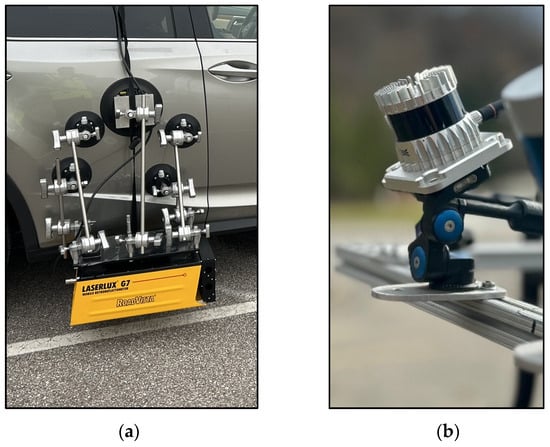
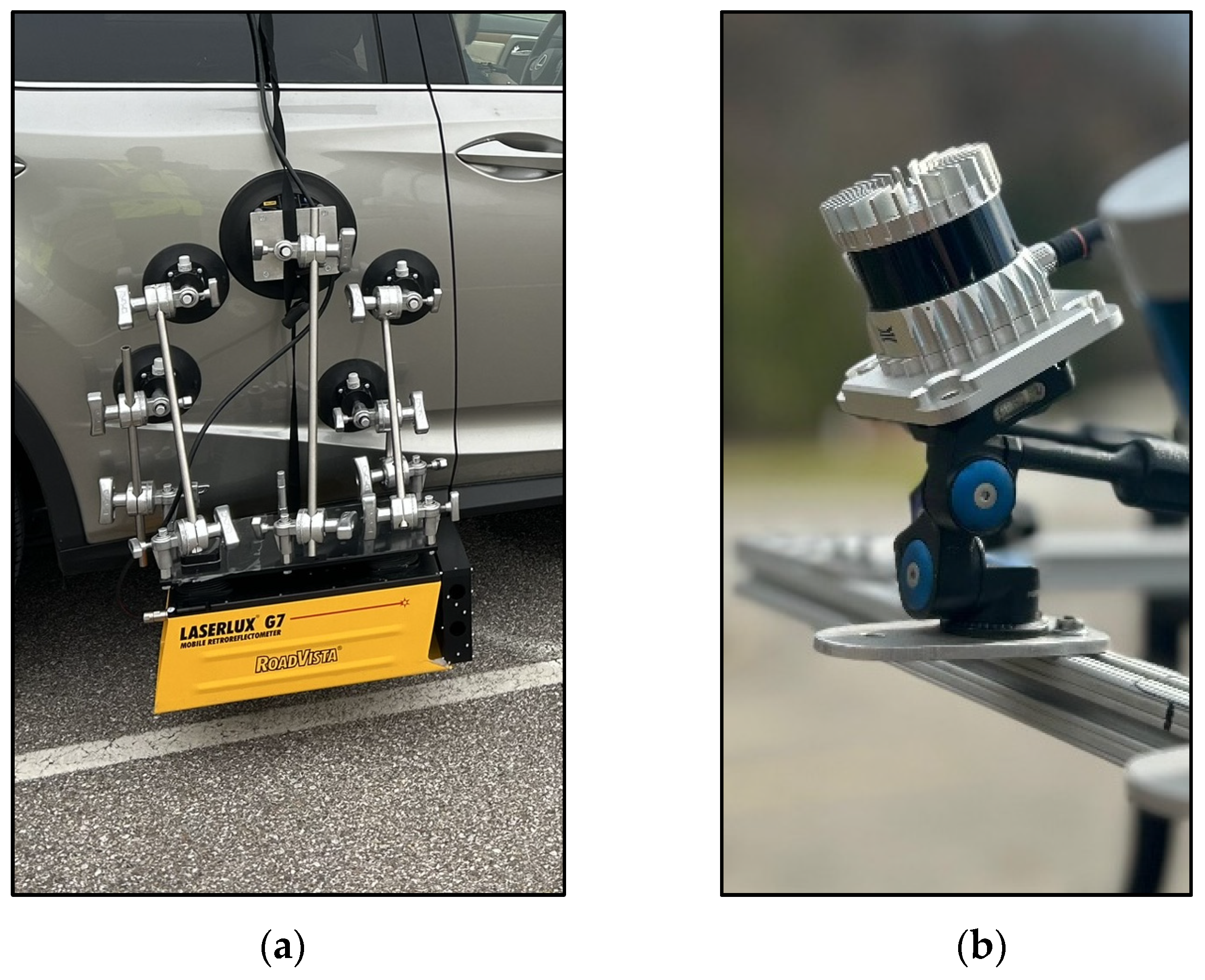
The RoadVista LLG7 (Gamma Scientific, San Diego, CA, USA) was selected for the Mobile Retroreflectometer Unit (MRU) due to its widespread use among DOTs and research teams, ensuring compatibility and consistency across projects. It gives detailed information not only about pavement marking retroreflectivity but also about surrounding conditions like temperature, humidity, and contrast. The selected sensors are illustrated in Figure 1, and their key specifications are summarized in Table 1.
Figure 1.
(a) The RoadVista LLG7 MRU (b) The Ouster OS1 LiDAR.
Table 1.
Key sensors specifications.
3.2. Sensors Placement
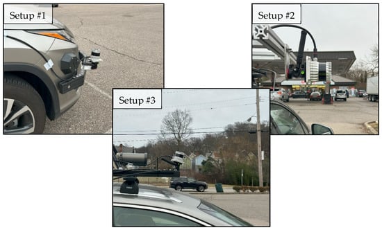
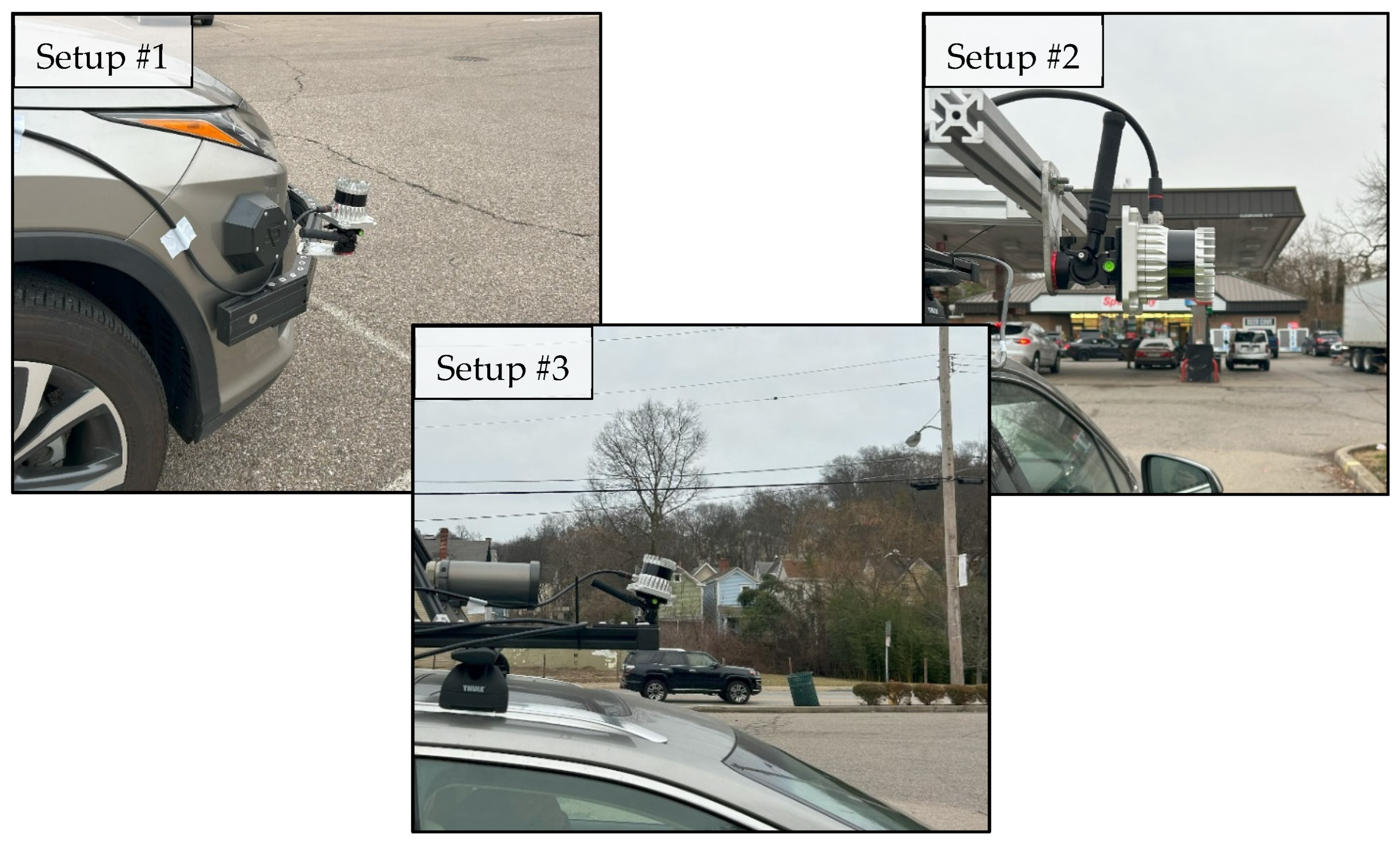
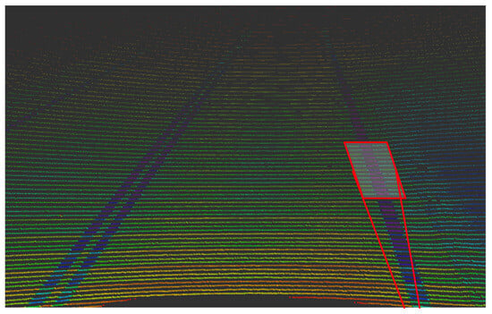
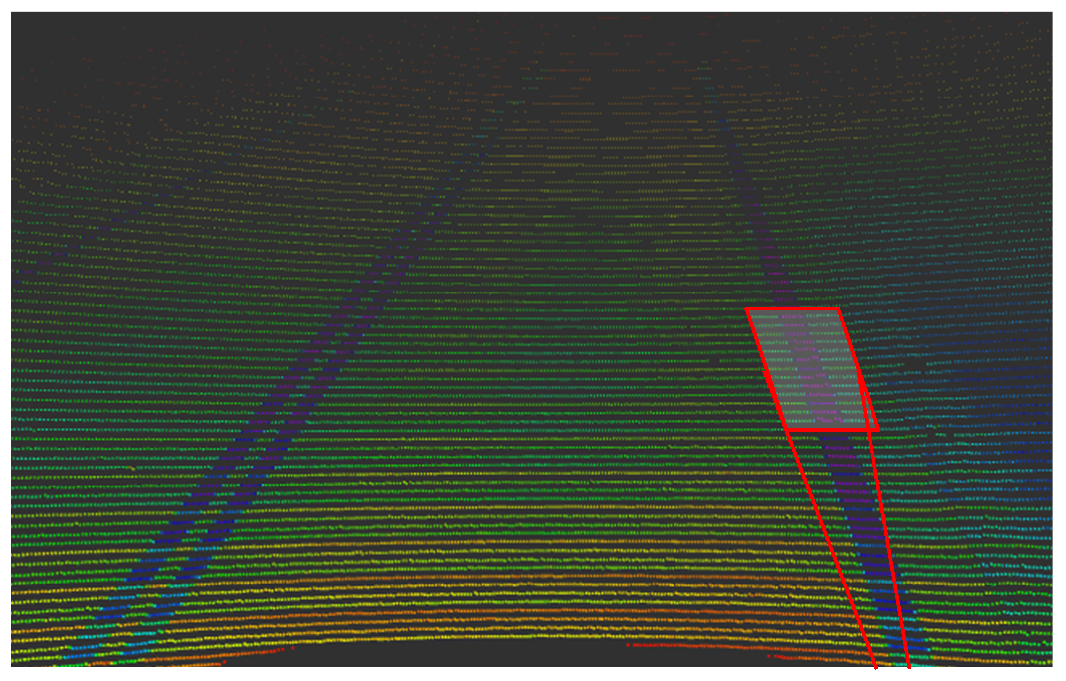
To determine the optimal location for mounting the OS1 LiDAR and define its data collection range, three different setups were tested, as shown in Figure 2. These configurations were designed to compare the LiDAR’s ability to scan the same pavement marking segment targeted by the LLG7, which was mounted on the right side of the vehicle to capture the right edge solid white line as seen in Figure 3, where the red box indicates the approximate MRU area of focus within the broader LiDAR field of view, and the color-coded point cloud represents LiDAR intensity values, with higher intensities shown in blue and purple.
Figure 2.
The three tested setups in various positions.
Figure 3.
Approximate MRU measurement area within the LiDAR field of view; the red box indicates the MRU focus area, and point cloud colors represent LiDAR intensity (higher intensity in blue and purple).
In Setup #1, the OS1 was installed on the right rear corner of the vehicle, 29 inches above the ground, and angled downward at 10°. In Setup #2, it was mounted on the right side of the vehicle and rotated 90° to directly face the lane marking. In Setup #3, the sensor was mounted on the top center of the vehicle, facing forward with a 15° tilt.
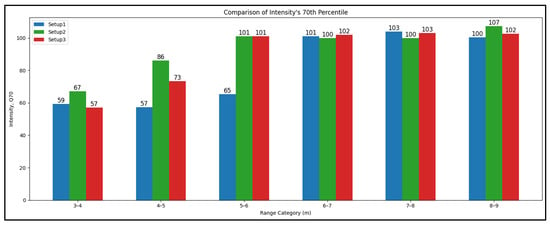
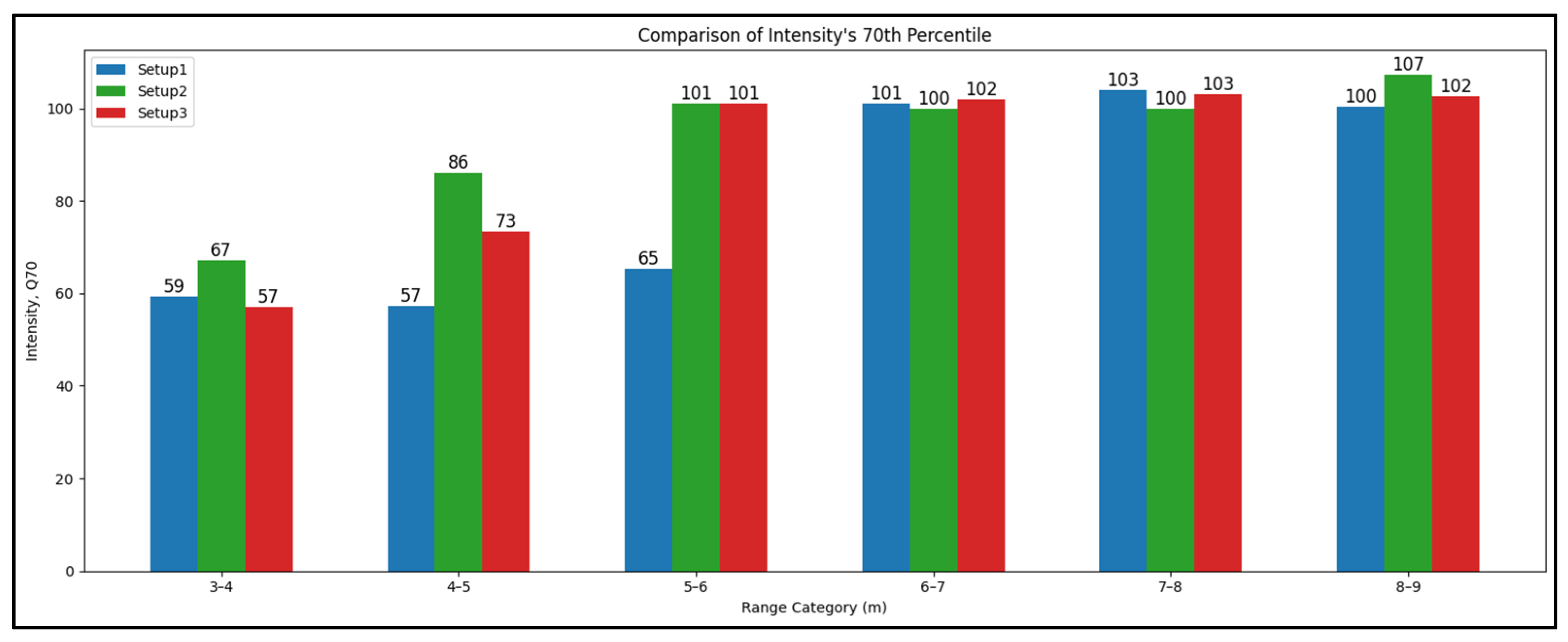
Two-way ANOVA was used to test the effect of the point cloud distance and the LiDAR setup on the intensity values. The dataset was divided into 6 distance categories (in meters); (3–4), (4–5), (5–6), (6–7), (7–8), (8–9). As seen in Table 2, the p-values for the Category and Setup variables are lower than 0.05, which means that the distance and setup configuration have significant effect on the intensity values.
Table 2.
Two-way ANOVA between distance category and LiDAR setup.
Before conducting the ANOVA, the normality of the residuals and the equality of variances were checked using the Shapiro–Wilk and Levene tests. The results indicated deviations from normality (p < 0.001) and non-homogeneous variances (p < 0.001). Since ANOVA is generally robust with large samples, a non-parametric Kruskal–Wallis test was also performed to confirm the findings, and it showed the same significance patterns, supporting the reliability of the ANOVA results.
Based on the previous findings, the first setup was removed from the dataset, and the test was done only on the distance categories between 5 and 8 m. According to the ANOVA results of the filtered dataset (Table 3), the intensity values are not affected by the distance in the 5-to-8-m range. That means that the intensity values are consistent in that range.
Table 3.
Two-way ANOVA between distance category and LiDAR setup, after removing setup #1 and only keeping (5–6), (6–7), (7–8) categories.
Figure 4 shows the consistency of the intensity values between the setups in the selected range. As shown in the figures, the points in setups 2 and 3 are consistently distributed along the trimmed range.
Figure 4.
Intensity vs. Range category.
The results from the second and third setup are similar and consistent in the 5–8-m range. However, the second setup can only be used to scan either the right side or the left side of the vehicle. Therefore, mounting the LiDAR on the top center of the vehicle as in the third setup is the best option to obtain consistent intensity values. This location best represents the reflectivity angle at which pavement markings are most visible to the driver. Also, 15° tilt reduces the spacing between the LiDAR channels in the area of interest, which increases the density of the point cloud.
3.3. Alignment and Synchronization
The alignment between the sensors is essential for creating a matched dataset that can be used to train reliable correlation models to predict pavement marking retroreflectivity from LiDAR intensity data. The model’s accuracy depends heavily on the quality and timing consistency of the input data.
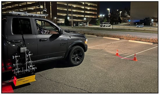
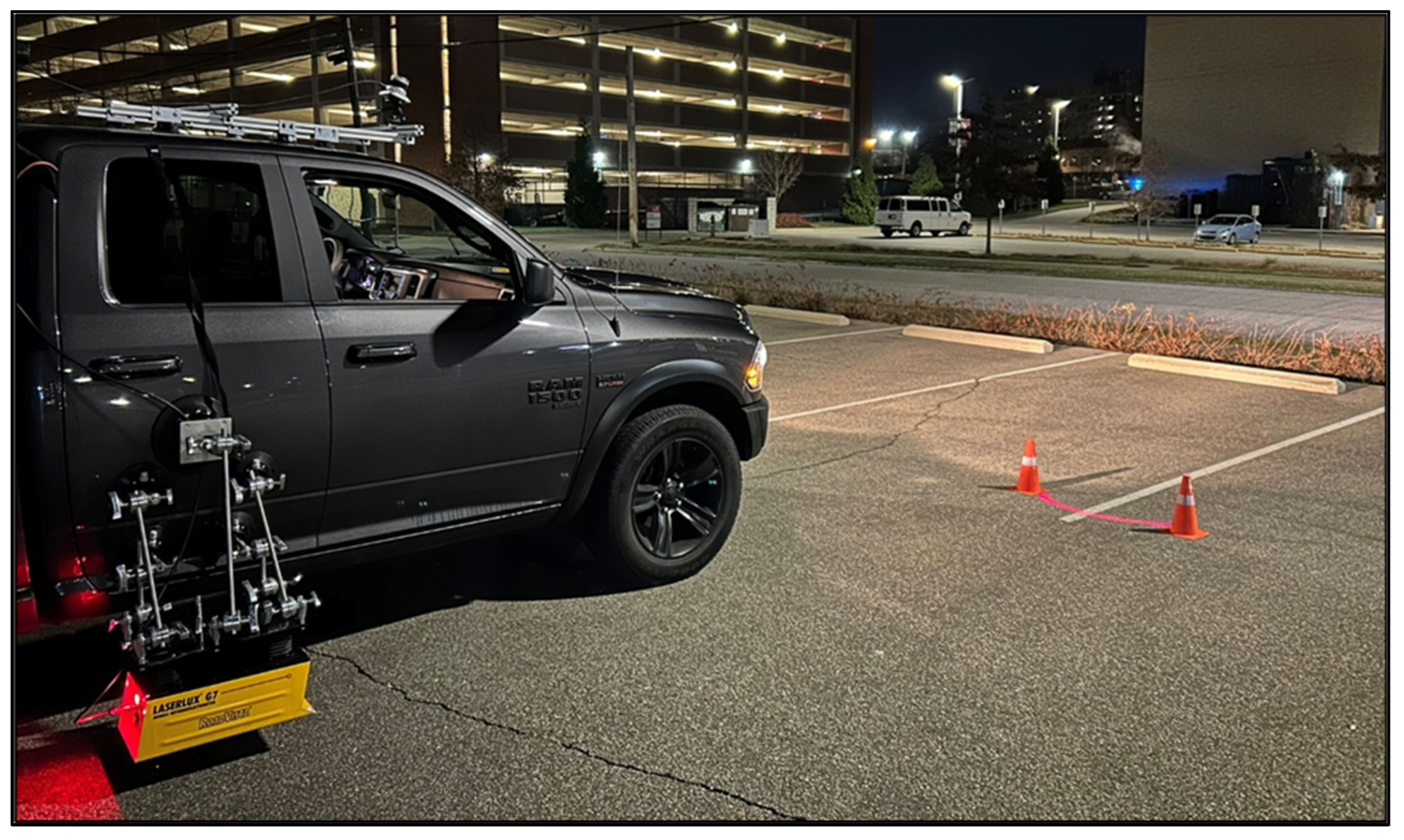
The MRU was mounted on the right side of the vehicle, and the LiDAR was mounted on top of the vehicle and tilted by 15° from the horizon to scan the lane marking in front of the vehicle. The laser from the MRU was visible on the ground in the night, making the process of determining the exact location of the measuring point easier. The measuring point was approximately 5.4 m from the MRU as seen in Figure 5.
Figure 5.
Estimation of the MRU’s scanning range.
The MRU was configured to record the average of every 5.28 ft to obtain the maximum number of points in the testing section. Even though both the MRU and LiDAR recorded the same distance, the number of points differs between the two devices. This discrepancy arises because the MRU data frequency is solely dependent on the driven distance. However, the LiDAR records data at a fixed frequency of 10 Hz, implying that the number of points is dependent on the speed of the vehicle.
To address this discrepancy, the LiDAR point cloud data was trimmed to record the same segment of the lane marking as the MRU. The sufficient overlapping between the consecutive LiDAR scans allowed for accurate synchronization between the points.
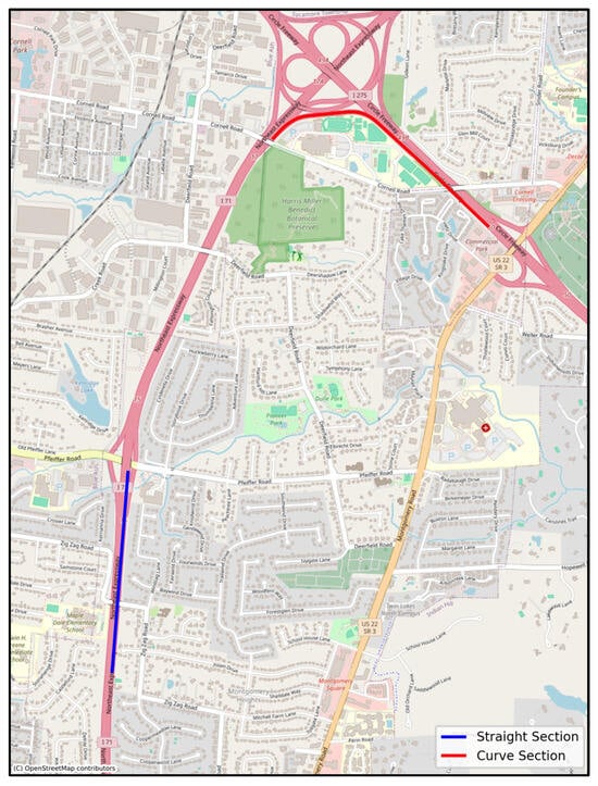
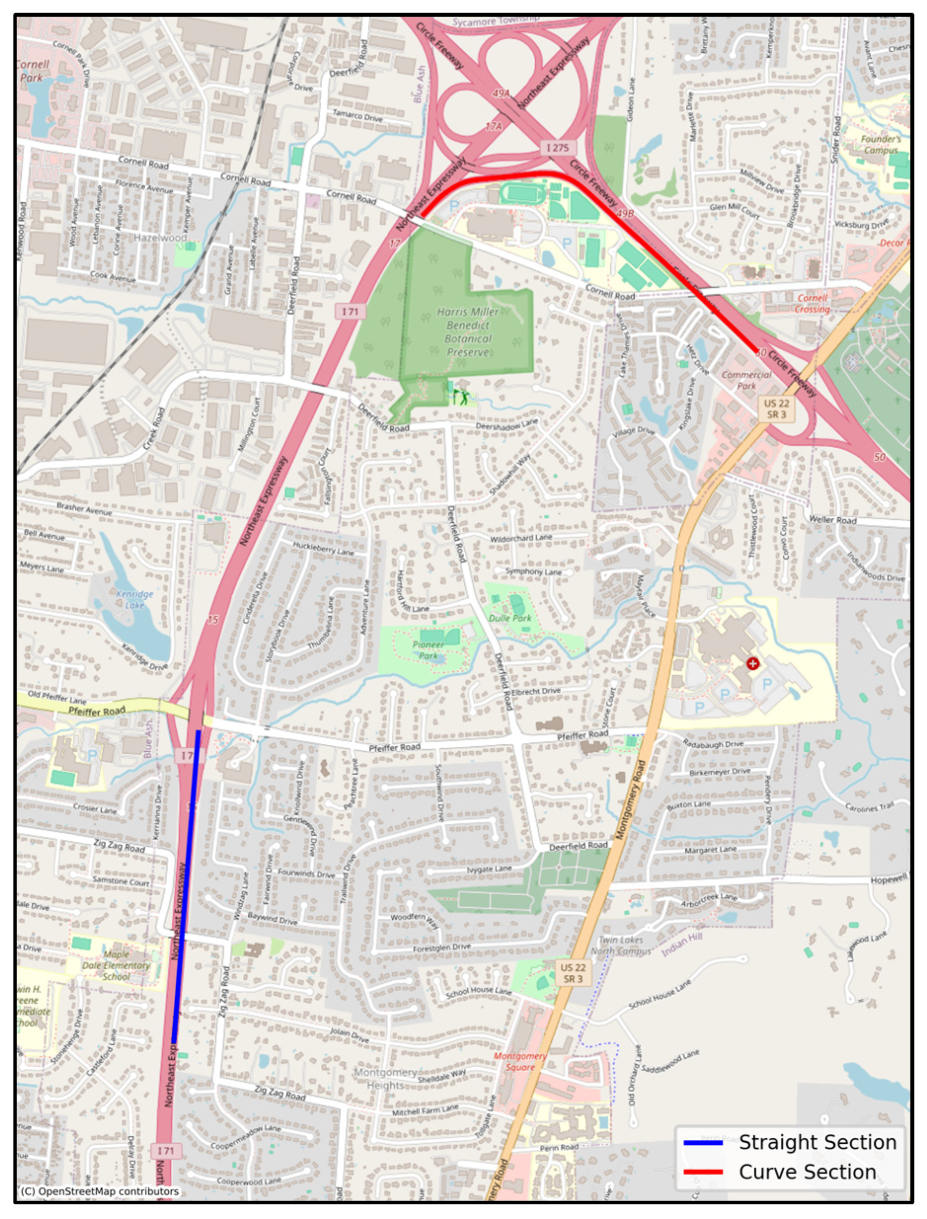
An experiment was carried out to explore how horizontal curves affect the synchronization process between the LiDAR and MRU. This experiment utilized two main sections (Figure 6): the first section, which was mostly straight with minimal horizontal curves, and the second section, containing both curved and straight portions.
Figure 6.
Curvature test sections.
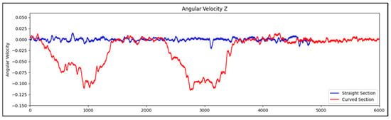
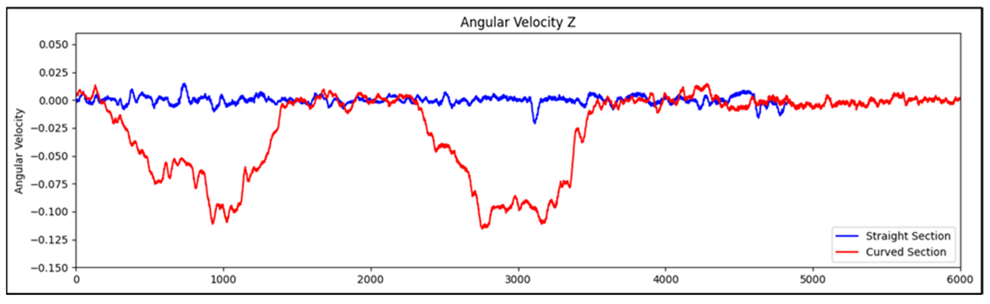
An Inertial Measurement Unit (IMU) was used to calculate the angular velocity around the z-axis, representing the turning speed of the vehicle. Figure 7 demonstrates the effect of horizontal curves on the IMU’s angular velocity around the z-axis. When the vehicle travels through a severe curve, the angular velocity around the z-axis increases or decreases significantly depending on the direction of the turn and the IMU’s mounting location in the vehicle. A right turn shows a negative angular velocity value, whereas a left turn shows a positive value. The extreme changes in angular velocity can cause misalignments between the LiDAR and MRU data points.
Figure 7.
Angular velocity around the z-axis changes along the tested sections.
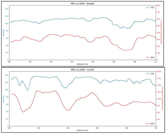
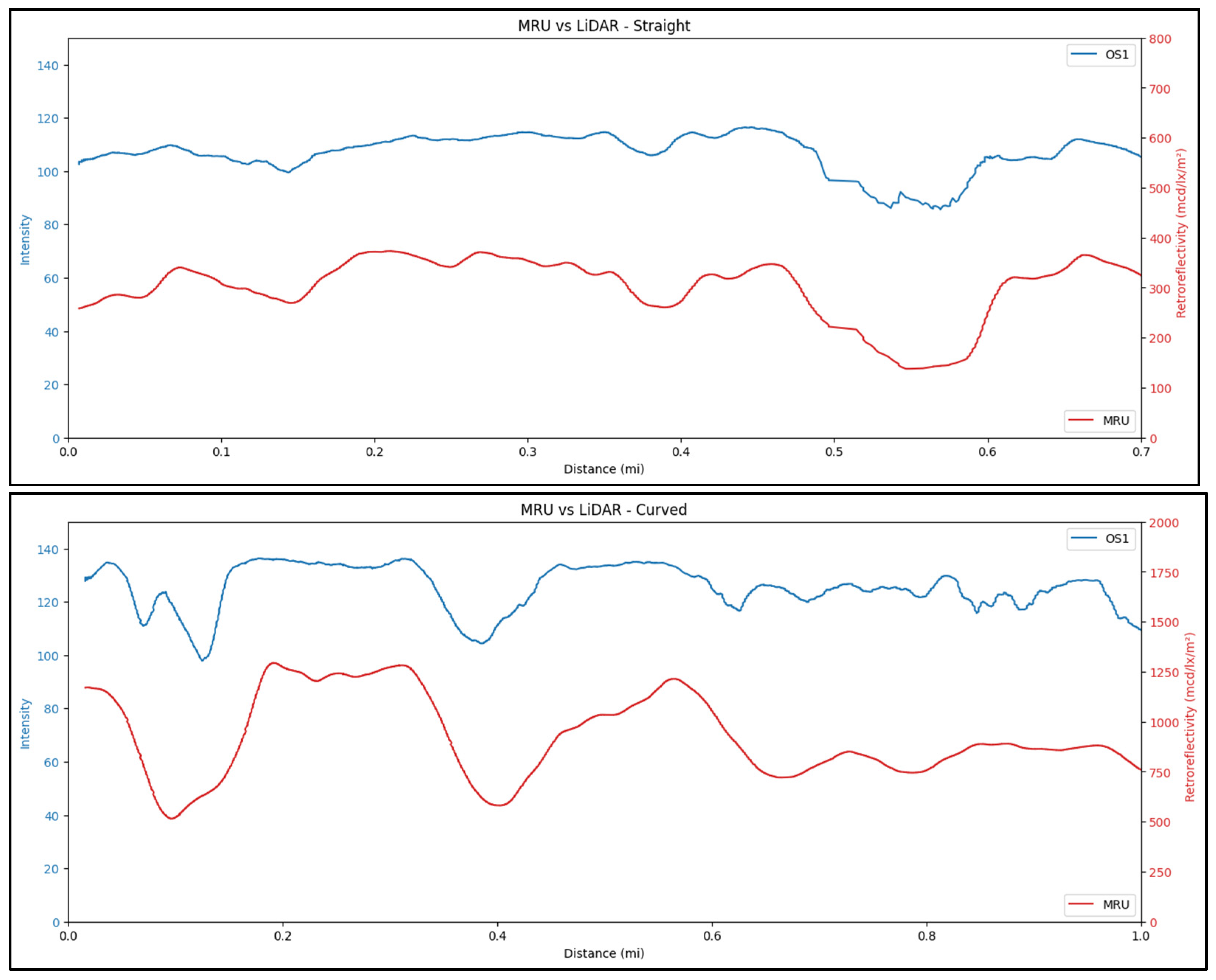
Figure 8 shows a visual comparison between the synchronization accuracy of the straight section and curved section. The curved section has clear discrepancies in the synchronization as compared to the straight section. Therefore, during the model’s development stage, the data points with high angular velocity values were removed to obtain a reliably matching dataset. However, when each device is implemented separately, this issue is no longer relevant.
Figure 8.
A visual comparison between the synchronization accuracy of the straight section and curved section.
3.4. Device Reading Repeatability
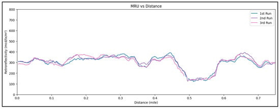
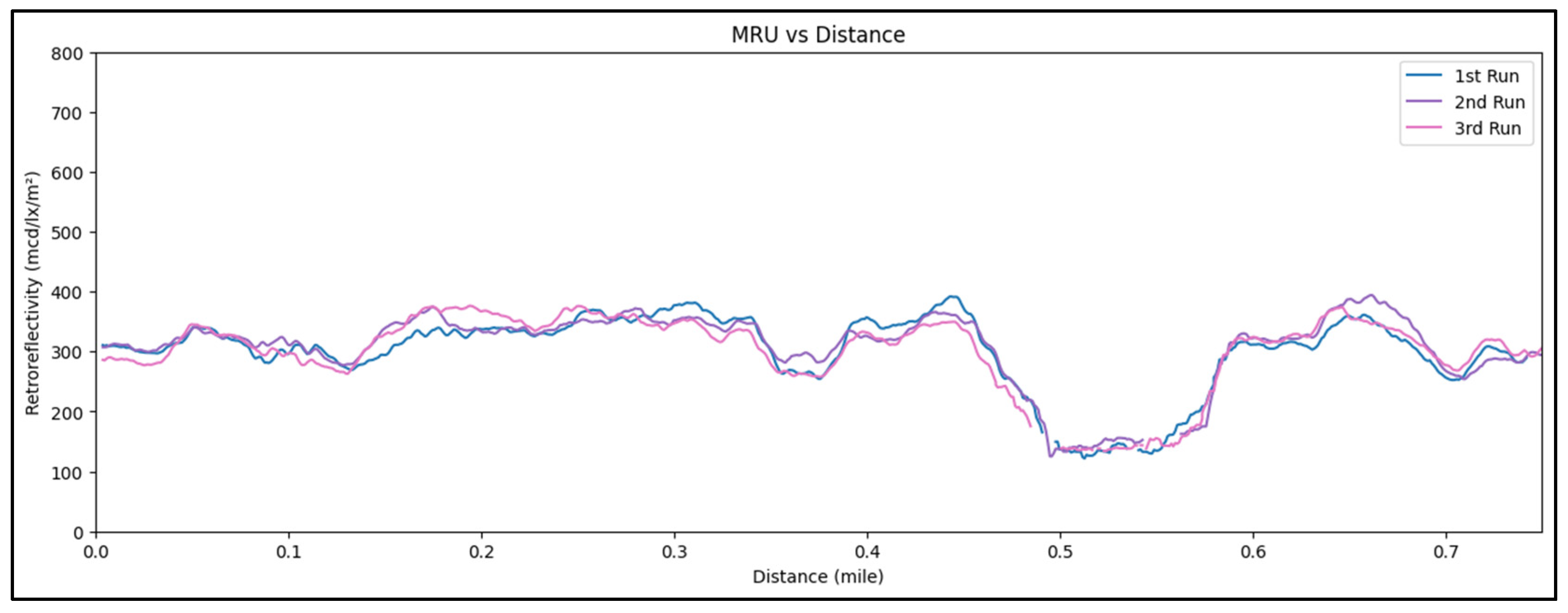
The repeatability and the reproducibility of the LiDAR and MRU were tested to verify that both devices give consistent measurements under the same conditions and that any future variation in the measurements is caused by the changes in the study parameters and conditions, not the sensors. Retroreflectivity and intensity measurements were collected over three separate runs along the same segment; the segment has a white solid edge line on the right side of the road. Figure 9 presents a comparison of retroreflectivity versus distance for all three runs, and the overlapping trends demonstrate a high level of consistency between the measurements. These results confirm that the MRU provides highly repeatable retroreflectivity measurements under consistent conditions.
Figure 9.
Retroreflectivity vs. distance plot for all three runs.
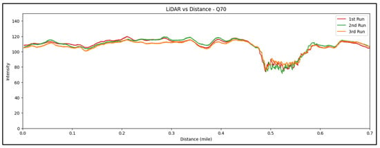
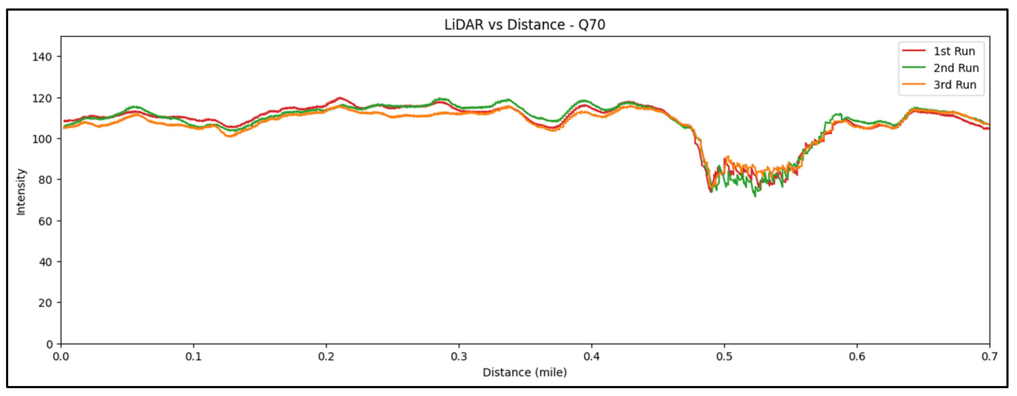
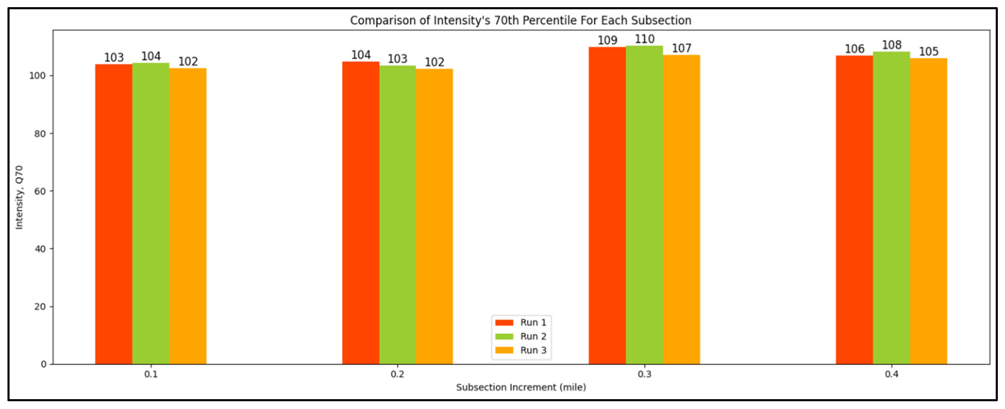
Figure 10 shows the comparison of intensity values versus distance for all three runs, and the overlapping trends clearly demonstrate a high level of consistency in the collected data. Additionally, Figure 11 shows a more detailed comparison, where intensity values were averaged every 0.1 mile to highlight consistency over smaller segments. The results confirm that the LiDAR sensor produces stable and repeatable intensity readings, supporting its reliability for pavement marking evaluation.
Figure 10.
Intensity vs. distance plot for all three runs.
Figure 11.
Intensity comparison between all runs, with values averaging every 0.1 miles to show detailed consistency.
3.5. Data Collection
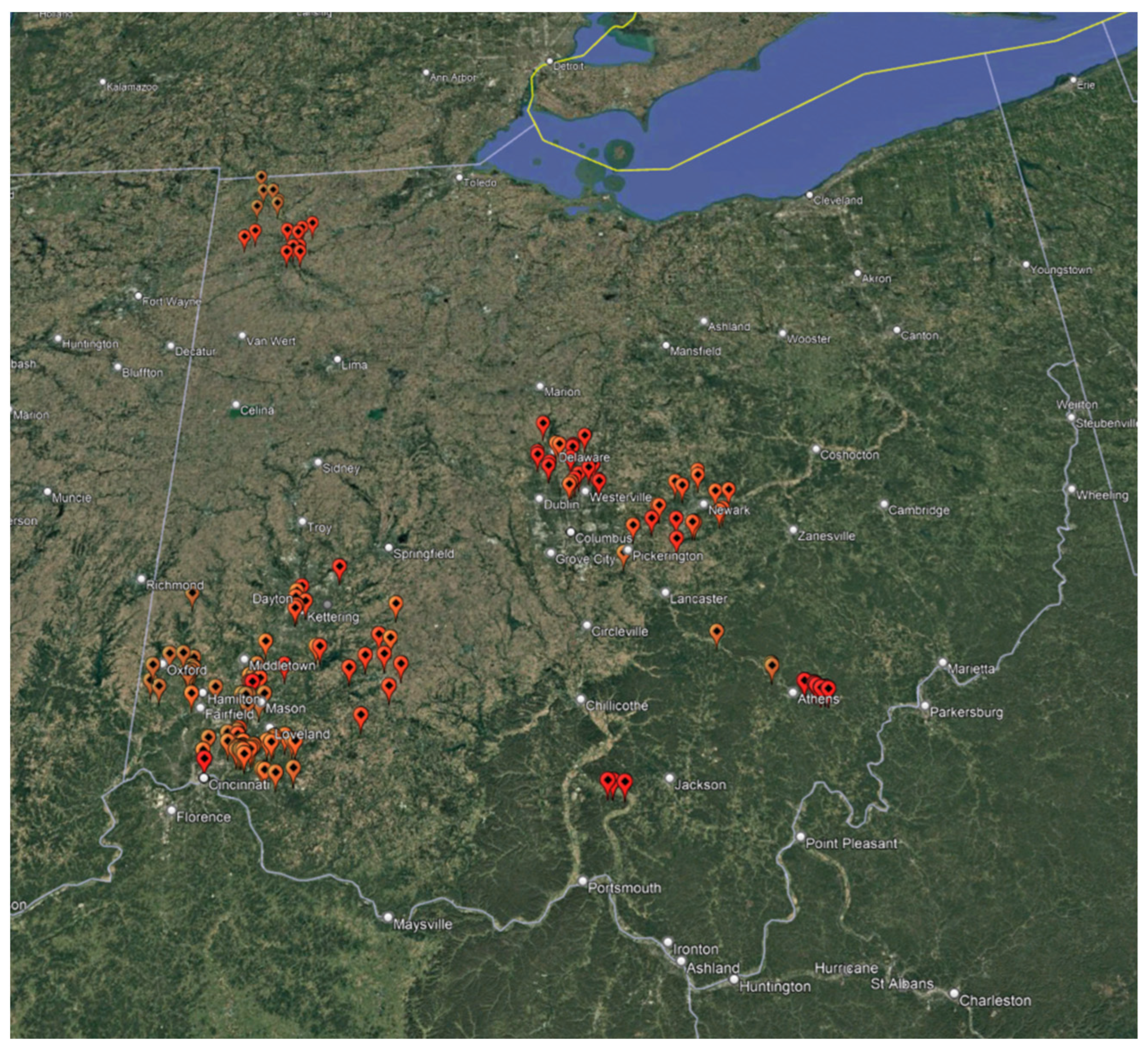
Developing a strong correlation model between LiDAR intensity and pavement marking retroreflectivity required a diverse and representative dataset. To achieve this, data was collected across a wide range of roadway types and marking conditions, including different colors and materials, such as white and yellow thermoplastic (from Swarco and 3M), polyurea, and high-reflectivity tape, as each type exhibits unique retroreflectivity characteristics. In total, more than 1000 miles of lane line data were collected, capturing the variability needed to train a reliable prediction model. Figure 12 demonstrates the overall map of the collected data.
Figure 12.
Google earth map of the collected data for the correlation models.
Although the total collected mileage was extensive, the dataset used for model development represents a refined subset of the available data. Emphasis was placed on roadway segments of greatest relevance to state transportation agencies. In addition, data influenced by road curvature, recording issues, or non-optimal sensor configurations were excluded. Together, these considerations ensured that the final dataset reflected consistent, high-quality measurements suitable for developing the correlation model.
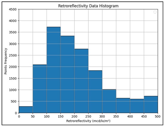
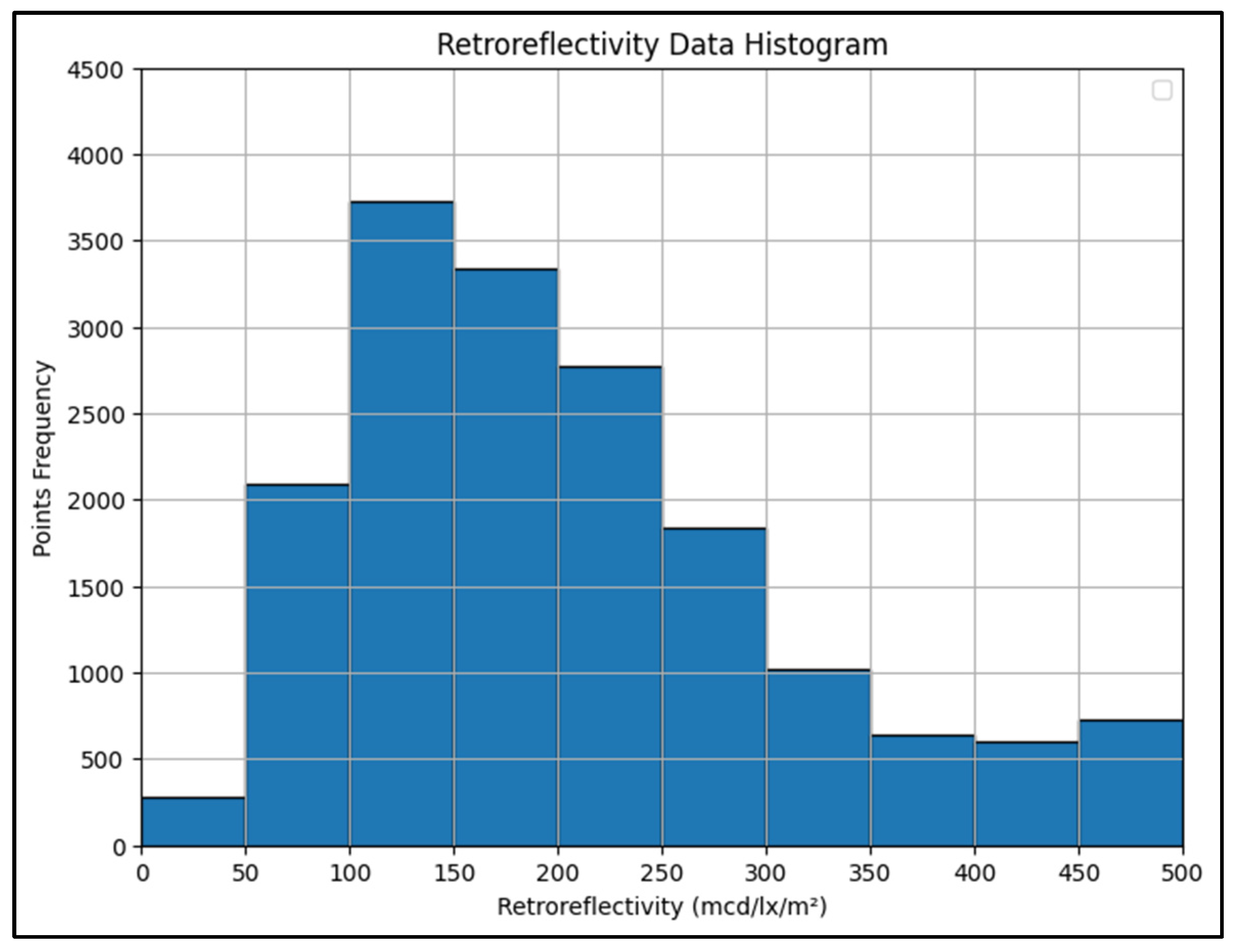
Figure 13 presents a histogram summarizing the distribution of retroreflectivity values across the filtered dataset. The frequency is expressed in terms of total points, showing how much pavement marking falls within each retroreflectivity range.
Figure 13.
Histogram of retroreflectivity values across the filtered dataset in total points per range.
The data reveals that the majority of the markings had lower retroreflectivity values, particularly between 50 and 300 mcd/lx/m2. This indicates that the pavement markings in the dataset predominantly exhibit moderate retroreflectivity levels, with fewer instances of very high values. This broad distribution is important for training a model that can accurately predict retroreflectivity across a wide range of conditions and pavement marking qualities.
3.6. Data Preparation
As previously shown, the LiDAR data was collected with the sensor facing forward with a 15° tilt, where the x-axis is parallel to the moving direction, the y-axis is transverse to the roadway. Therefore, the data was adjusted to obtain a horizontal road surface. The rotation process used here is adapted from the literature [15].
The rotation step aligns the raw point cloud with the vehicle’s coordinate system, ensuring that the LiDAR data reflects the actual orientation of the senor during data collection.
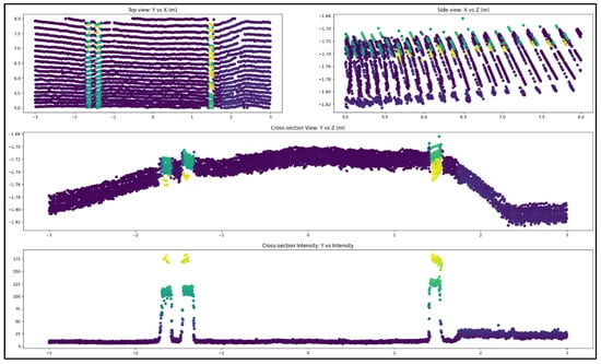
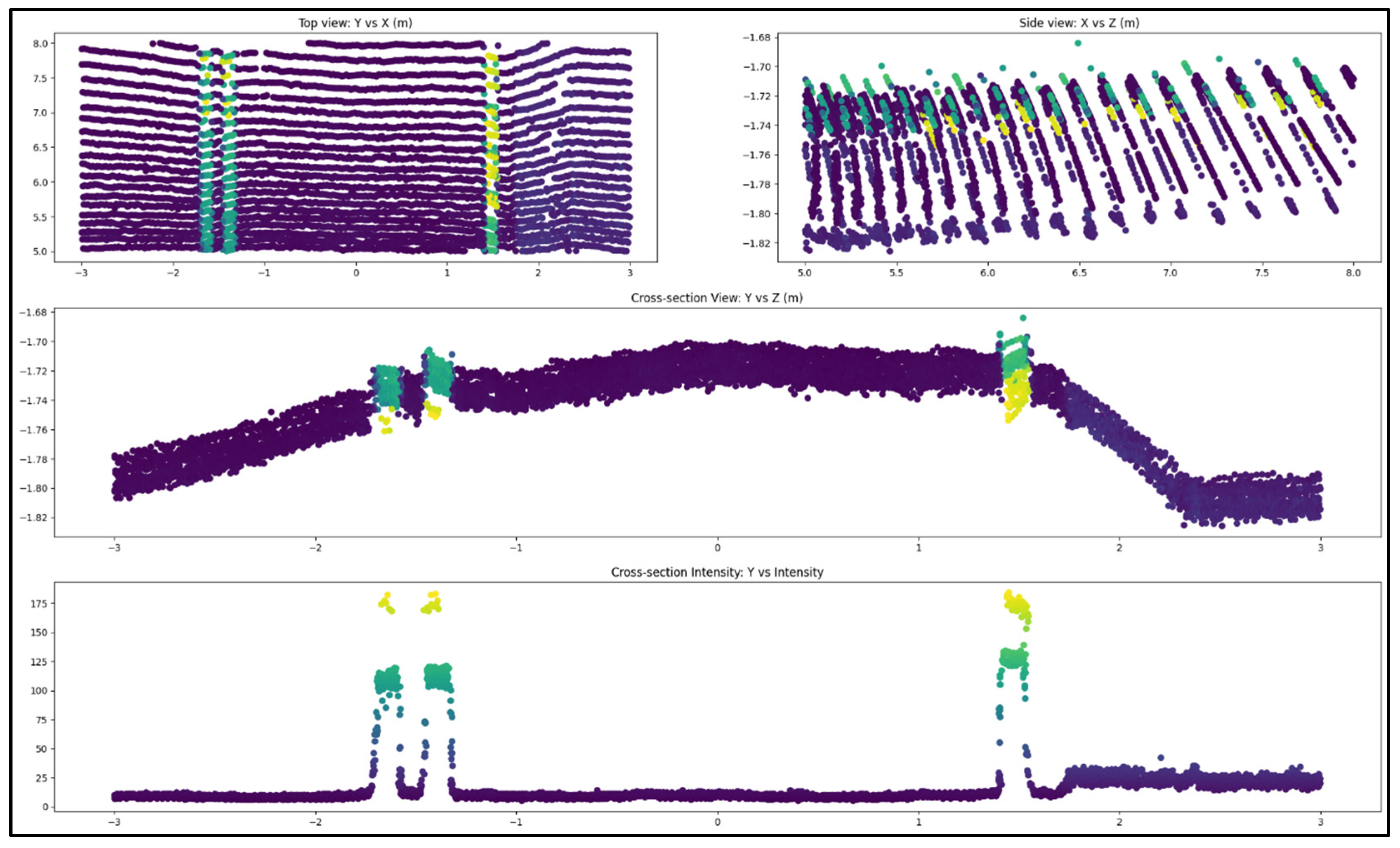
An example of the top, cross-sectional, and cross-section intensity views of a single scan are shown in Figure 14. To extract the lane marking data points from the LiDAR scans, a process based on rasterization was implemented to simplify manual segmentation. Rasterized graphs of the top view were used to segment the lane marking at each control point in the data. The raster image limits were independent from the point cloud used to plot it, so that each pixel in the rasterized image was exactly matched to the dimensions in the original graph.
Figure 14.
Top, cross-section, and cross-section intensity views of a preprocessed OS1 LiDAR scan, with point colors indicating intensity (higher in yellow and green for markings; lower in purple for pavement).
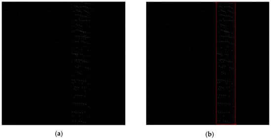
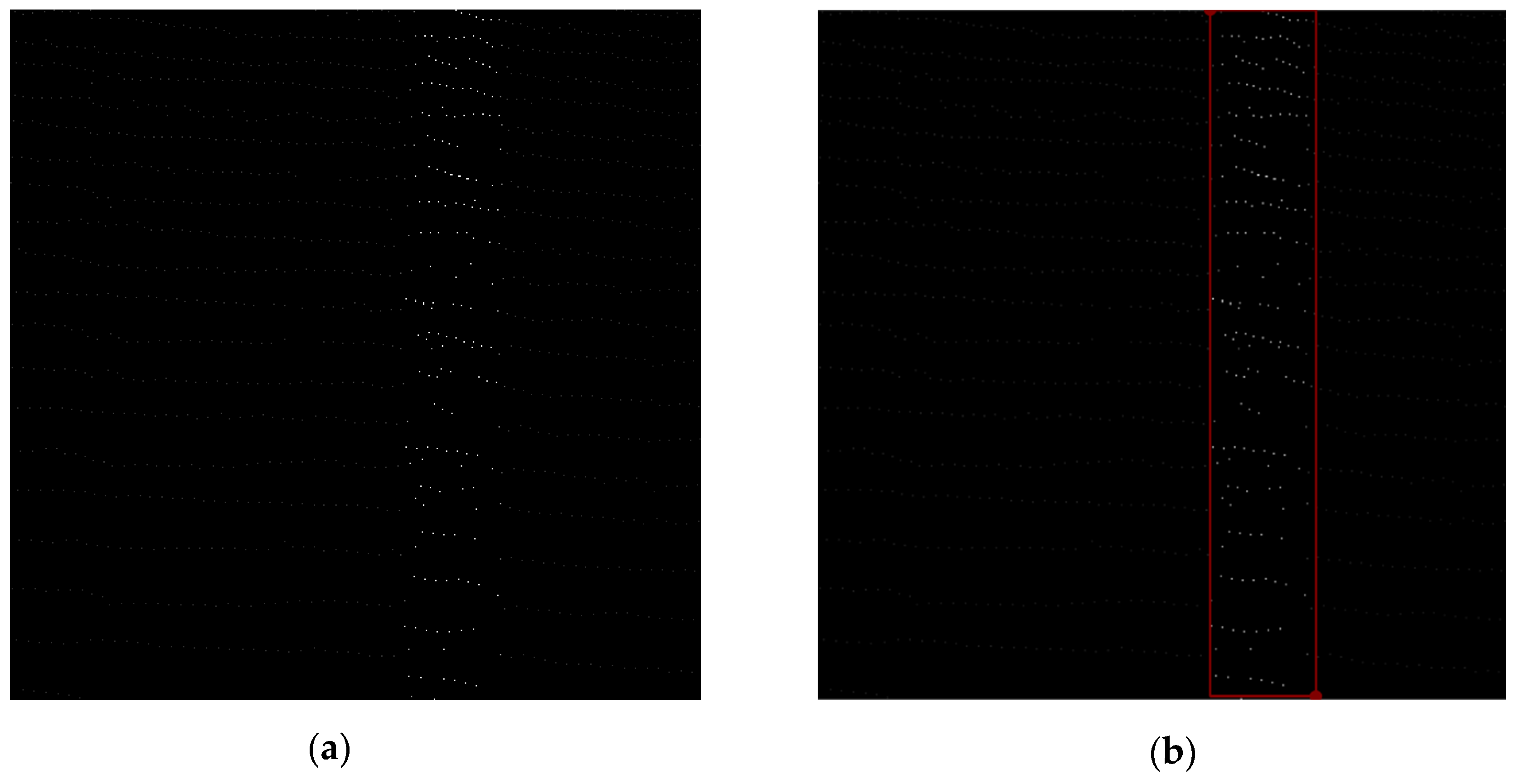
During the data collection, the scans were precisely centered at the measurement window. For precision, the raster images were specifically centered on the lane under examination as seen in Figure 15a, where the white dots represent points with higher LiDAR intensity. Emphasis during annotation was placed exclusively on the area proximate to the MRU’s active measuring zone. The dimensions of these annotation boxes are typically 4 inches in width demonstrated in Figure 15b, where the red lines indicate the annotation box. Subsequently, these annotations were then mapped back to the 3D point-cloud domain to capture the relevant points within the designated area.
Figure 15.
(a) Extracted raster image, (b) Annotated raster image.
3.7. Feature Extraction and Selection
The number of LiDAR points is not a constant and it can vary between scans, and since most predictive models require a uniform size, the raw data can’t be directly used for model training. To achieve this, key features are extracted from each scan to represent the point cloud. These features provide a uniform input size while preserving the information needed for accurate retroreflectivity correlation development.
Initially, over 200 features were extracted from each subset to represent the LiDAR data. Most of these features were based on the intensity values of the points, which are directly related to surface reflectivity. Additional features incorporated the spatial position of the points within the full point cloud, using their x and y coordinates. This combination helped capture both the brightness and the geometric distribution of the pavement markings.
To reduce dimensionality and redundancy among the initially extracted 212 features, an exploratory feature screening procedure was applied, following the general principles described in [16]. The selection process combined quantitative analysis with expert-guided interpretation, rather than relying on a single automated optimization method. Pairwise scatter plots and correlation coefficients were first examined to identify features exhibiting strong redundancy, limited variability, or unstable behavior across samples. In addition to these analytical measures, features were evaluated based on their physical interpretability and relevance to pavement marking reflectivity and spatial structure, informed by domain knowledge and empirical observations from prior studies.
Features conveying overlapping information or demonstrating limited discriminative potential were progressively removed through this combined assessment, resulting in a final subset of 32 complementary features. All feature screening steps were conducted using training data only and were completed prior to model evaluation to avoid information leakage.
The selected features captured key statistical and signal characteristics of the LiDAR intensity data, including measures of central tendency, variability, and distribution shape (mean, standard deviation, skewness, kurtosis). Trend and change indicators such as moving averages, gradients, slopes, and curvature describe local variations. Rolling window statistics further highlighted localized variations along pavement markings.
3.8. Correlation Models Training
To find the best model for predicting retroreflectivity from LiDAR data, a variety of regression techniques were tested. The evaluation began with basic linear regression models, which aimed to capture simple relationships in the data while using regularization to prevent overfitting. More advanced machine learning models were also explored, including Decision Tree and Random Forest, which are well-suited for handling non-linear patterns and can highlight important features in the dataset. To further improve prediction accuracy, boosting models such as Gradient Boosting (scikit-learn v1.3.2), XGBoost (v2.0.3), and LightGBM (v4.3.0) were used. These models work by combining multiple weak learners to iteratively improve predictions, making them highly effective for complex datasets.
During model development, key hyperparameters such as max_depth, min_samples_split, min_samples_leaf, max_leaf_nodes, and learning_rate were tuned to reduce overfitting and improve predictive accuracy.
The models were assessed based on their R2 scores and median relative error. After evaluating the performance of each model, an ensemble approach was used to predict the pavement marking retroreflectivity by combining the outputs of three different models. Each model independently predicted retroreflectivity values, and the final output was calculated as the average of the three predictions. Averaging predictions from the three models reduces individual errors, balances over- and underestimations, and minimizes the impact of outliers. This ensemble approach integrates their strengths to deliver balanced, reliable, and consistent retroreflectivity predictions. Table 4 shows the final tuned hyperparameters for the key models, which were selected using a limited, expert-guided search based on prior experience, commonly used values in the literature, and preliminary experiments.
Table 4.
Tuned hyperparameters for the key machine learning models.
3.9. Correlation Models Validation
The correlation models were validated on approximately 30 miles of roadway segments that were not used during model training, ensuring an independent evaluation of model performance. These sections included interstates, state routes, and county roads, providing a good mix of road types. The validation areas were spread across several regions, representing a range of conditions and locations.
To accurately evaluate the model’s performance, the predicted retroreflectivity values were grouped into 0.1-mile segments for each validation section. This segmentation minimizes the impact of large variability in retroreflectivity across an entire section, ensuring a more precise and meaningful comparison between predicted and actual values as the MRU typically measures the retroreflectivity every 0.1 mile.
3.10. Prediction Repeatability
To evaluate the consistency in retroreflectivity prediction, a 1.2 miles segment on the I-71 was recorded three times. The segment contained solid and dashed markings, with a high range of retroreflectivity values. The intensity value from each run was used to calculate the retroreflectivity separately.
4. Results and Discussion
4.1. Models Training Results
The final dataset contained 18,784 data points after completing all preprocessing steps. To evaluate model performance, the data was divided into training and testing sets using an 80:20 split, ensuring that the models were trained on the majority of the data while still being tested on a separate portion to assess their predictive accuracy.
As described in Section 3.2 and Section 3.3, each scan is trimmed to optimize stability of readings and matching with MRU, therefore, most of the area segmented from each scan is totally different than the one scanned before. Nonetheless, there is an intentional small region of overlap to provide buffering. However, because the splitting is scan-based (time and location different), this means that the small overlap region across two consecutive scans are two completely different readings from two different angles. Therefore, the presence of this overlap doesn’t present a risk for model overfitting or performance inflation. Second, and most importantly, the performance of the model on the test dataset is only used as an intermediary step during the model training phase and not to validate the actual measurable performance in the field or to evaluate the presented approach. This is why the performance of the developed system is evaluated on completely new sections never seen by the model during any phase of the development as described in the validation section.
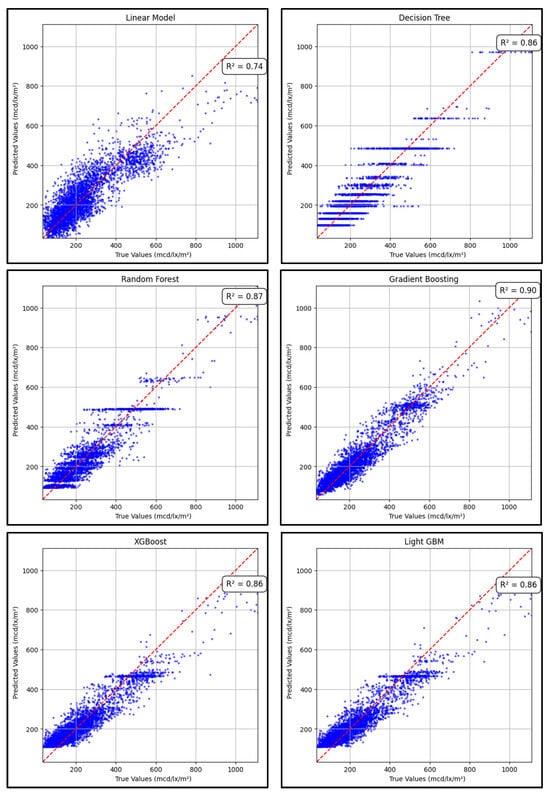
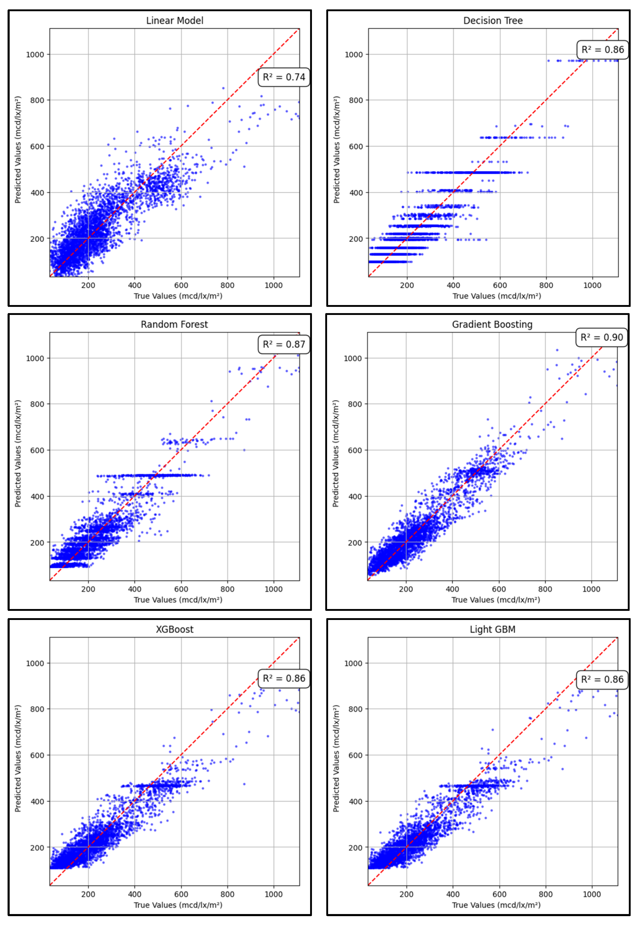
The performance of the regression models was evaluated to determine their effectiveness in predicting pavement marking retroreflectivity from LiDAR data. Figure 16 and Table 5 summarize the results from both training and testing datasets.
Figure 16.
Predicted vs. true retroreflectivity values for the trained regression models.
Table 5.
Testing R2, training R2, and median relative error for each model.
Gradient Boosting outperformed all other models, achieving the highest testing R2 of 0.90 and the lowest relative error of 11.8%, indicating strong predictive accuracy. Random Forest followed closely with an R2 of 0.87 and a relative error of 12.8%. Decision Tree, XGBoost, and LightGBM all performed similarly with R2 scores of 0.86, while Linear Regression showed the lowest accuracy with an R2 of 0.74 and a higher relative error of 19.3%.
After testing and evaluating various combinations of models, the ensemble of the Gradient Boosting, XGBoost, and LightGBM models resulted in the best performance. These results highlight the advantage of using ensemble methods, particularly boosting techniques, for modeling the complex relationship between LiDAR intensity and retroreflectivity.
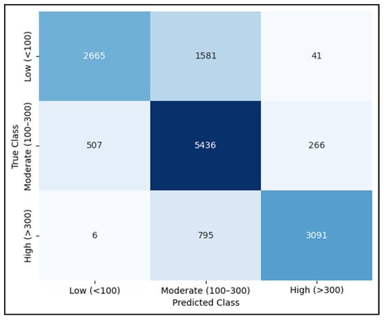
A confusion matrix was generated using the validation set to evaluate how well the model identifies pavement markings within operationally meaningful retroreflectivity ranges. As shown in Figure 17, the ensemble model performs reliably across the three retroreflectivity categories: low (<100), moderate (100–300), and high (>300 mcd/lx/m2). Most moderate and high retroreflectivity points are correctly classified, and only a small number of samples near category boundaries are misclassified. Although low retroreflectivity markings represent a small portion of the dataset, the matrix provides a direct view of the model’s behavior in this critical range and adds practical insight into its potential use for maintenance decision-making.
Figure 17.
Confusion matrix showing the model’s classification performance across the three retroreflectivity ranges (<100, 100–300, >300 mcd/lx/m2), with color intensity indicating relative frequency.
4.2. Feature Importance
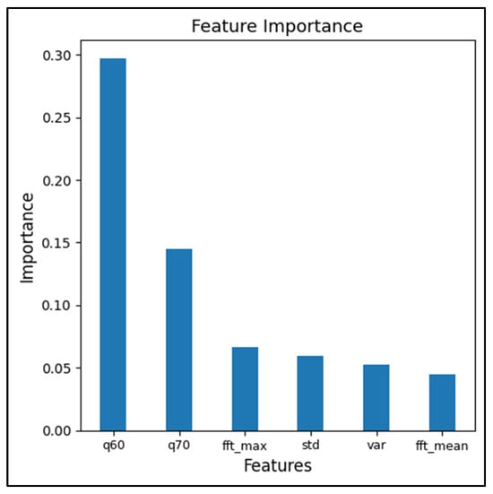
After training the machine learning models, the LiDAR intensity-based features that influenced the retroreflectivity prediction the most were identified. The importance factor highlighted which statistically and spatial characteristics of the intensity had the greatest impact on model performance.
The feature importance results showed that the 60th percentile (q60) and 70th percentile (q70) of LiDAR intensity had the most significant impact on the predicted values, followed by maximum Fast Fourier Transform amplitude (fft_max), standard deviation (std), variance (var), and the mean Fast Fourier Transform amplitude (fft_mean). The high importance factor of the percentile intensity features indicates that the middle portion of the intensity distribution provides the closest representation of pavement marking retroreflectivity, while the frequency features (fft_max and fft_mean) represent the signal variations in the data. The importance factor of the top 6 features is shown in Figure 18.
Figure 18.
The top 6 features impacting the retroreflectivity predictions.
4.3. Models Validation Results
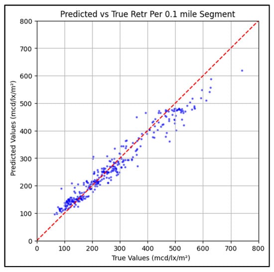
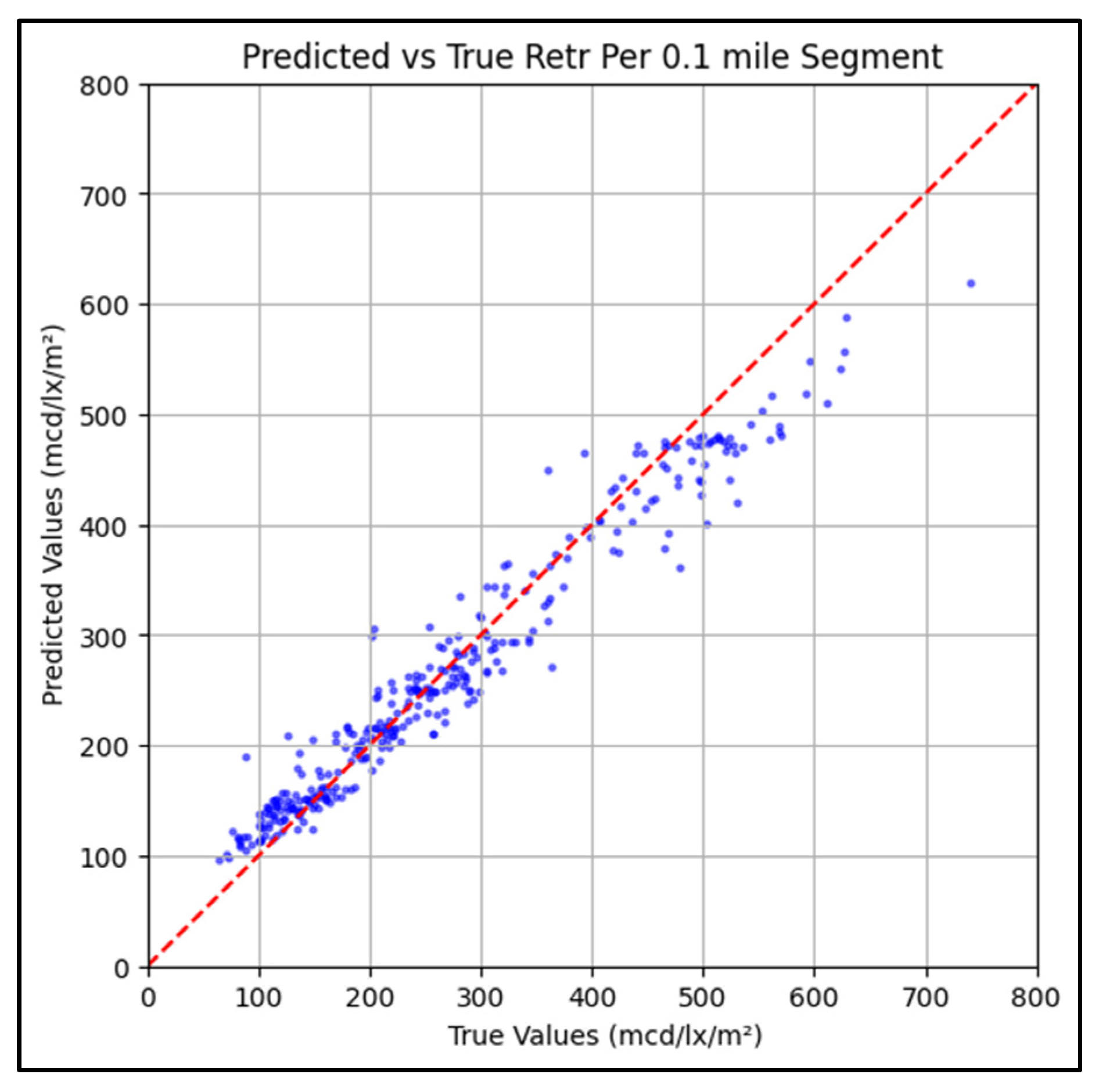
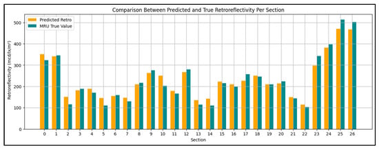
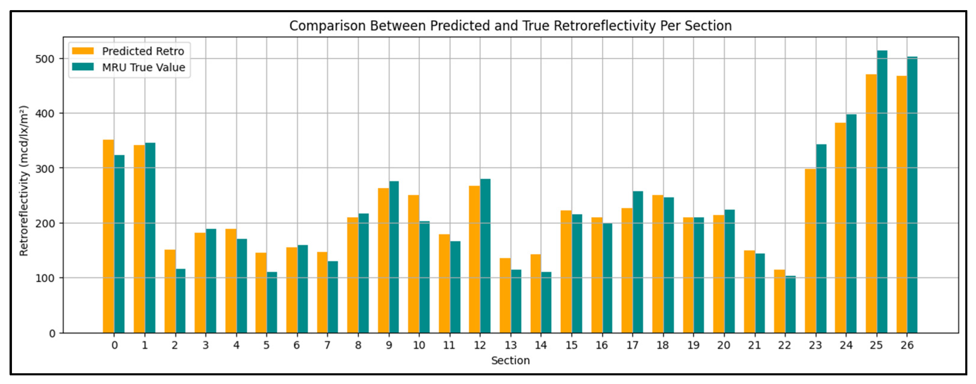
As described in the methodology, the validation was performed on 30 miles of sections never seen before and not used during feature selection or model tuning. The model demonstrates strong overall performance, with a low mean absolute and a typical error magnitude (RMSE). As seen in Table 6, the mean absolute percentage error (11.55%) shows minimal deviation relative to true values. Additionally, the high R2 score and strong correlation coefficient indicate excellent alignment between predicted and true retroreflectivity values, highlighting the model’s reliability and accuracy. The scatter plot in Figure 19 shows strong alignment between predicted and true retroreflectivity values, with most points near the 1:1 line, indicating accurate and consistent model performance. The bar chart in Figure 20 shows a summarized comparison between the predicted and true retroreflectivity for each section.
Table 6.
Ensemble model performance metrics.
Figure 19.
Predicted vs. true retroreflectivity values per 0.1-mile for the validation sections.
Figure 20.
Comparison between predicted and measured MRU retroreflectivity per section.
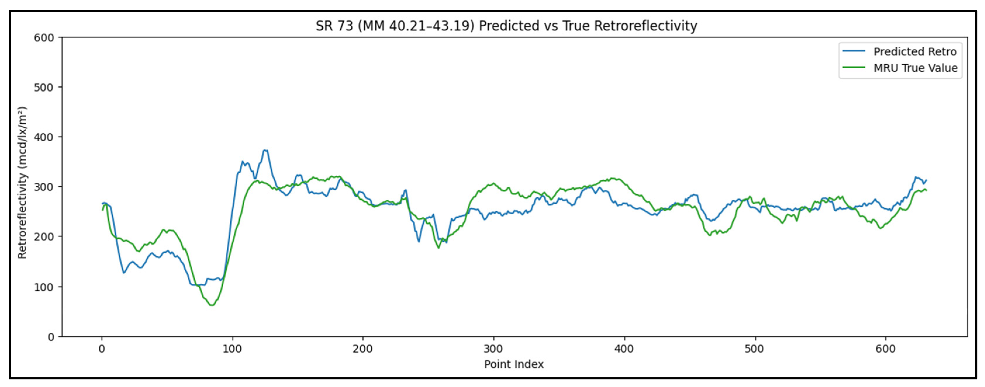
The trend in Figure 21 shows a comparison between the predicted and MRU measured retroreflectivity values along a sample validation section. The detailed trend illustrates the accuracy of the predicated retroreflectivity values as well as the precise alignment between the points.
Figure 21.
Predicted vs. MRU measured retroreflectivity values along a sample validation section, SR 73.
4.4. Prediction Repeatability Results
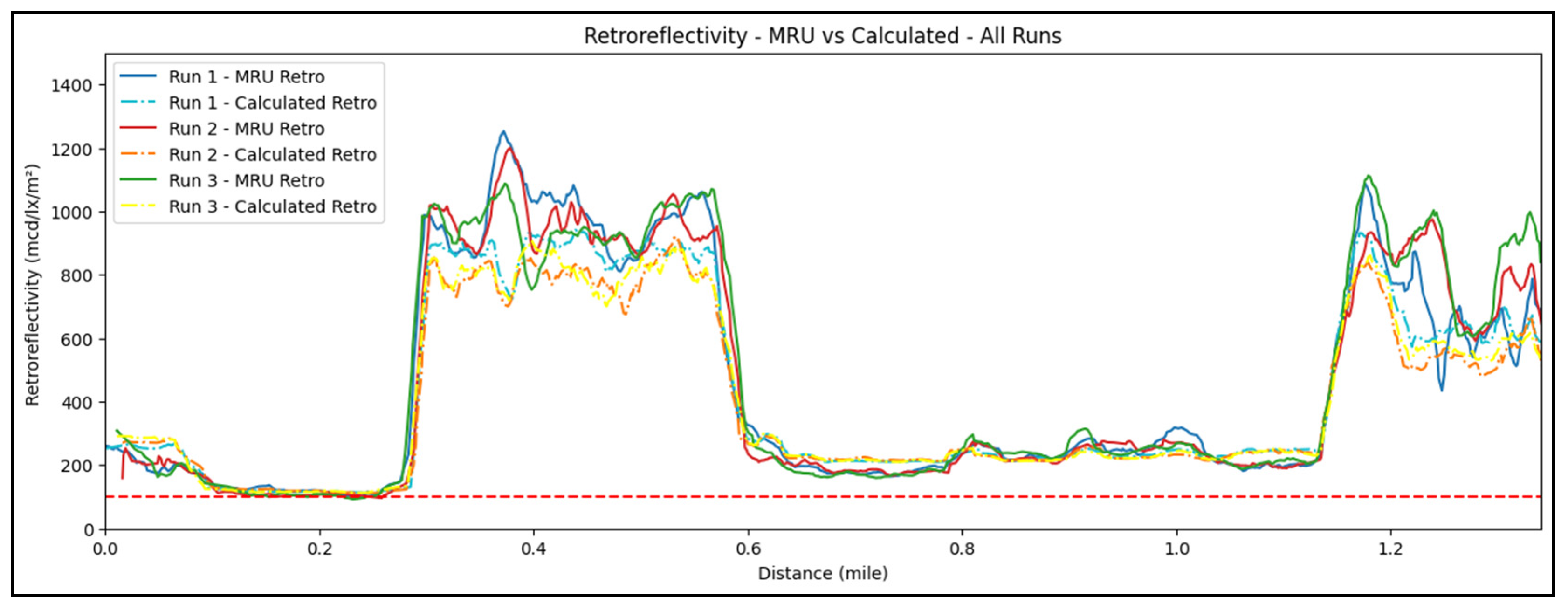
The predicted retroreflectivity was more consistent as compared to the retroreflectivity measured by the MRU. This is caused by the high variability in the MRU values as compared to a more consistent intensity value, especially at high retroreflectivity segments. Figure 22 shows a comparison between the predicted retroreflectivity values from each run.
Figure 22.
Comparison between the predicted retroreflectivity values from each run, where the red dashed line shows the FHWA minimun retroreflectivity limit of the tested road (100 mcd/lx/m2).
5. Conclusions
This paper focused on developing and validating models to predict pavement marking retroreflectivity using LiDAR intensity data. The retroreflectivity correlation models showed strong performance, with Gradient Boosting achieving an R2 of 0.90 and good accuracy on validation sections. These results demonstrate the reliability and consistency of the correlation across various road types, materials, and marking conditions.
- Three LiDAR mounting setups were tested in this research; Setup 3 (top center) was found to provide the most consistent and practical intensity data across the 5–8 m range.
- Accurate synchronization between the LiDAR and MRU is crucial for ensuring a well-aligned dataset and achieving reliable correlation between LiDAR intensity and retroreflectivity measurements.
- Points at curved road segments were removed only because of alignment issues between the LiDAR and MRU, which adapt differently to curvature; however, this does not limit the final model, as both sensors operate reliably on curves when used independently.
- Both the LiDAR and MRU demonstrated high repeatability and consistency across multiple runs under the same conditions.
- The percentile-based LiDAR intensity features, particularly q60 and q70, were identified as the most important predictors of pavement marking retroreflectivity, highlighting the strong influence of mid-range intensity values on model performance.
- Gradient Boosting showed the best individual performance (R2 = 0.90, 11.8% error), and when combined with XGBoost and LightGBM in an ensemble, the model achieved high consistency (R2 = 0.94, MAPE = 11.5%), confirming LiDAR’s strong potential for scalable retroreflectivity evaluation.
- The predicted retroreflectivity values were highly consistent across runs, showing less variation than the MRU measurements and demonstrating the stability of LiDAR based predictions.
- The approach developed in this study can further improve road safety by allowing rapid detection and maintenance of the low retroreflectivity areas in the marking network, which will provide vehicles with sufficient and adequate nighttime visibility on the road.
6. Limitation and Future Work
- The analysis was conducted using dry condition pavement data only, because the MRU cannot operate reliably on wet or rainy surfaces. As a result, the model has not been evaluated under wet weather conditions. Future work should examine the correlation and model performance under wet or rainy conditions to determine robustness beyond dry weather operation.
- While the model captures the overall relationship between LiDAR intensity and retroreflectivity, detailed performance differences among marking types, materials, colors, and road categories were not analyzed, as they fall outside the scope of this study. Future studies should examine model behavior across specific marking materials, colors, installation methods, and roadway categories to better understand inter-category performance.
- The developed correlation is limited by several factors, including the dependence of LiDAR intensity on sensor configuration, and the fact that the developed correlation is specific to the LiDAR system used in the study.
Author Contributions
The authors confirm contribution to the paper as follows: Conceptualization: M.N. and D.M.; data collection: H.B.; analysis and interpretation of results: M.N., H.B. and D.M.; draft manuscript preparation: M.N., H.B., D.M. and A.A. All authors have read and agreed to the published version of the manuscript.
Funding
This research work presented in this paper was part of study funded by the US Federal Highway Administration and the Ohio Department of Transportation, State Job Number: 136667.
Data Availability Statement
The datasets presented in this article are not readily available because they are part of an ongoing study.
Conflicts of Interest
The authors declared no potential conflicts of interest with respect to the research, authorship, and/or publication of this article.
Abbreviations
The following abbreviations are used in this manuscript:
| MRU | Mobile Retroreflectometer Unit |
| LiDAR | Light Detection and Ranging |
| MAPE | Mean Absolute Percentage Error |
| FHWA | Federal Highway Administration |
| MUTCD | The Manual on Uniform Traffic Control Devices |
| GNSS | Global Navigation Satellite Systems |
| GPS | Global Positioning System |
| RL | Retroreflectivity |
| LLG7 | LaserLux G7 |
| IMU | Inertial Measurement Unit |
| DOT | Department of Transportation |
| TEM | Traffic Engineering Manual |
References
- Ward, J.; Hall, C.; Robertson, J.; Durdin, P.; Smith, D.; Green, D. Guide to Traffic Management Part 10: Traffic Control and Communication Devices; Austroads Ltd.: Sydney, Australia, 2019. [Google Scholar]
- El Krine, A.; Girard, J.; Redondin, M.; Heinkele, C.; Stresser, A.; Muzet, V. Road Marking Characterization for ADAS Machine Vision Reliability. In Proceedings of the 31st European Safety & Reliability Conference (ESREL), Angers, France, 19–23 September 2021. [Google Scholar] [CrossRef] [Scilit]
- Jiang, L.; Huang, Y.; Li, H.; Li, F. An Innovative Road-Marking Quality-Assessment Mechanism Using Computer Vision. Adv. Mech. Eng. 2016, 8, 1687814016654043. [Google Scholar] [CrossRef] [Scilit]
- Federal Highway Administration. Final Rule: Maintaining Minimum Pavement Marking Retroreflectivity. Federal Register, 5 August 2022; p. 87.
- Pike, A.M.; Barrette, T. Evaluation of the Effects of Pavement Marking Retroreflectivity on Nighttime Visibility; NCHRP Project 20-102(06), Final Report; Transportation Research Board: Washington, DC, USA, 2018. [Google Scholar]
- Babić, D.; Babić, D.; Ščukanec, A.; Lazarić, M.; Dragčević, V.; Barić, D. Impact of Road Marking Retroreflectivity on Machine Vision-Based Lane Support Systems. Sensors 2022, 22, 1303. [Google Scholar] [CrossRef] [Scilit] [PubMed]
- Bektas, B.A.; Gkritza, K.; Smadi, O. Pavement marking retroreflectivity and crash frequency: Segmentation, line type, and imputation effects. J. Transp. Eng. 2016, 142, 04016030. [Google Scholar] [CrossRef] [Scilit]
- Roy, U.; Albatayneh, O.; Ksaibati, K. Pavement Marking Practices, Standards, Applications, and Retroreflectivity. Transp. Res. Rec. 2023, 2677, 564–576. [Google Scholar] [CrossRef] [Scilit]
- ASTM E3320-21; Standard Guide for Mobile Retroreflectivity Measurement of Pavement Markings Using Imaging Technology. ASTM International: West Conshohocken, PA, USA, 2021.
- Federal Highway Administration. Manual on Uniform Traffic Control Devices (MUTCD), 2009th ed.; Rev. 3, July 2022; FHWA: Washington, DC, USA, 2022. [Google Scholar]
- Texas Department of Transportation. Technical Memorandum: FY 2021 Mobile Retro (Verification Report); Texas DOT: Austin, TX, USA, 2022. [Google Scholar]
- Florida Department of Transportation. FM 5-600: Florida Test Method for Measuring Retroreflectivity of Pavement Markings Using a Mobile Retroreflectometer; Florida DOT: Tallahassee, FL, USA, 2023. [Google Scholar]
- Minnesota Department of Transportation. Pavement Marking Retroreflectivity Inspection Methods: Research Implementation Committee Handbook (RIC 2024-05H); Minnesota DOT: St. Paul, MN, USA, 2024. [Google Scholar]
- Federal Highway Administration. Every Day Counts (EDC-6) Final Report; U.S. Department of Transportation, FHWA: Washington, DC, USA, 2022. [Google Scholar]
- Manasreh, D. Towards the Application of Autonomous Vehicle Technology in Transportation Infrastructure Asset Assessment. Doctoral Dissertation, University of Cincinnati, Cincinnati, OH, USA, 2023. Available online: http://rave.ohiolink.edu/etdc/view?acc_num=ucin1704980557328935 (accessed on 11 January 2026).
- Manasreh, D.; Nazzal, M.D.; Abbas, A.R. Feature-Centric Approach for Learning-Based Prediction of Pavement Marking Retroreflectivity from Mobile LiDAR Data. Buildings 2024, 14, 62. [Google Scholar] [CrossRef] [Scilit]
- Soilán, M.; González-Aguilera, D.; del-Campo-Sánchez, A.; Hernández-López, D.; Del Pozo, S. Road Marking Degradation Analysis Using 3D Point Cloud Data Acquired with a Low-Cost Mobile Mapping System. Autom. Constr. 2022, 141, 104446. [Google Scholar] [CrossRef] [Scilit]
- Hou, Q.; Ai, C.; Boudreau, N. An Automated Pavement Marking Retroreflectivity Condition Assessment Method Using Mobile LiDAR and Video Log Images. J. Infrastruct. Syst. 2024, 30, 04024004. [Google Scholar] [CrossRef] [Scilit]
- Ai, C.; Hennessy, E. A Pavement Marking Inventory and Retroreflectivity Condition Assessment Method Using Mobile LiDAR; Rep. No. 22-030; Massachusetts Dept. of Transportation, Office of Transportation Planning: Boston, MA, USA, 2022. Available online: https://rosap.ntl.bts.gov/view/dot/63369 (accessed on 11 January 2026).
- Mahlberg, J.A.; Cheng, Y.T.; Bullock, D.M.; Habib, A. Leveraging LiDAR Intensity to Evaluate Roadway Pavement Markings. Future Transp. 2021, 1, 720–736. [Google Scholar] [CrossRef] [Scilit]
- Olsen, M.J.; Parrish, C.; Che, E.; Jung, J.; Greenwood, J. LiDAR for Maintenance of Pavement Reflective Markings and Retroreflective Signs; Rep. No. FHWA-OR-RD-19-01; Oregon Dept. of Transportation: Salem, OR, USA, 2018. Available online: https://rosap.ntl.bts.gov/view/dot/36526 (accessed on 11 January 2026).
- Pedregosa, F.; Varoquaux, G.; Gramfort, A.; Michel, V.; Thirion, B.; Grisel, O.; Blondel, M.; Prettenhofer, P.; Weiss, R.; Dubourg, V.; et al. Scikit-Learn: Machine Learning in Python. J. Mach. Learn. Res. 2011, 12, 2825–2830. [Google Scholar]
- Chen, T.; Guestrin, C. XGBoost: A Scalable Tree Boosting System. In Proceedings of the 22nd ACM SIGKDD International Conference on Knowledge Discovery and Data Mining, San Francisco, CA, USA, 13–17 August 2016; pp. 785–794. [Google Scholar] [CrossRef] [Scilit]
- Ke, G.; Meng, Q.; Finley, T.; Wang, T.; Chen, W.; Ma, W.; Ye, Q.; Liu, T.-Y. LightGBM: A Highly Efficient Gradient Boosting Decision Tree. In Proceedings of the 31st International Conference on Neural Information Processing Systems, Long Beach, CA, USA, 4–9 December 2017; Volume 30, pp. 3146–3154. Available online: https://proceedings.neurips.cc/paper/2017/file/6449f44a102fde848669bdd9eb6b76fa-Paper.pdf (accessed on 11 January 2026).

Disclaimer/Publisher’s Note: The statements, opinions and data contained in all publications are solely those of the individual author(s) and contributor(s) and not of MDPI and/or the editor(s). MDPI and/or the editor(s) disclaim responsibility for any injury to people or property resulting from any ideas, methods, instructions or products referred to in the content. |
© 2026 by the authors. Licensee MDPI, Basel, Switzerland. This article is an open access article distributed under the terms and conditions of the Creative Commons Attribution (CC BY) license.