Intelligent Steel Surface Defect Segmentation for Edge-Oriented IIoT Quality Control

Abstract

Automated surface defect detection in hot-rolled steel is a prerequisite for real-time quality control, yet most deployed inspection systems operate in isolation from Industrial Internet of Things (IIoT) infrastructure. This paper reports a laboratory-scale proof of concept with two contributions. The first is a segmentation study on the Severstal dataset using a leakage-free, defect-stratified split of 1886 test images. Because a trivial all-background predictor already attains 96.66% pixel accuracy, performance is reported through Dice, IoU, precision, recall, and F1 with 95% confidence intervals. A compact from-scratch U-Net (0.49 M parameters) reaches a Dice of 0.416 at 38.6 ms per image, an ImageNet-pretrained DeepLabV3+ model reaches 0.677 at 46.3 ms and 37 times the parameters, and a classical Otsu baseline reaches 0.060, bracketing an explicit accuracy-versus-footprint design space rather than a single recommended model. The second contribution is architectural: a three-layer IIoT architecture whose messaging layer is empirically characterized on a Raspberry Pi broker over 158,500 messages. A factorial experiment isolates the transport configuration of the broker, rather than that of the publisher, as the determinant of end-to-end latency, yielding a seventeen-fold reduction. The layer sustains 1920 messages per second without loss, and a deliberate broker outage shows that MQTT delivery guarantees are semantic rather than temporal, motivating an application-level message-expiry policy. Embedded inference deployment is identified as the primary next step.

1. Introduction

The steel industry is one of the most economically and strategically relevant sectors in Brazil and worldwide. Brazil, as the ninth largest global steel producer and the largest in Latin America, operates a park of 31 plants with an annual installed capacity of approximately 51 million tons [1]. Within this productive context, the quality of steel surfaces constitutes a competitive differentiator, particularly for special steels destined for automotive, aerospace, and construction applications.

Surface defects such as scratches, cracks, and scale inclusions arise during the hot rolling process as a direct consequence of mechanical deformation, thermal cycling, and contact with rolling equipment such as rolls and guide rails [2]. Traditional quality control in steel plants relies on manual visual inspection and laboratory chemical and physical sampling, procedures that are widely reported to be inadequate to guarantee defect-free surfaces [3] and prone to errors under the harsh conditions of continuous production [4]; this reliance inherently delays defect detection and may result in substantial material waste when defective lots are only identified after completing the rolling sequence. The resulting demand for automated, image-based inspections has motivated a substantial body of research in recent decades [5]. Human visual inspection, while widely practiced, presents known reliability limitations, with detection accuracy varying substantially across inspectors, defect types, and operating conditions.

Automated computer vision systems address these limitations but face their own deployment barriers in legacy industrial environments including the following: high acquisition costs, rigid installation requirements, and limited integration with modern connectivity infrastructure. Furthermore, most deployed inspection systems operate in isolation, without any mechanism for real-time data sharing with process control, maintenance, or quality management systems. This isolation prevents the use of predictive analytics and data-driven process optimization [6].

The emergence of deep learning, particularly convolutional neural networks (CNNs) and the encoder–decoder architecture known as U-Net [7], provides a technically mature basis for automated pixel-level defect segmentation. At the same time, the Industrial Internet of Things (IIoT) offers a connectivity layer that allows local inference results to be aggregated, stored, and analyzed at scale. The convergence of these two technologies creates a practical pathway toward intelligent, low-latency quality monitoring on the production floor.

This paper makes two contributions. The first is experimental. We train a compact U-Net on the publicly available Severstal Steel Defect Detection dataset and evaluate it on a leakage-free, defect-stratified test set of 1886 images, reporting the Dice coefficient, IoU, precision, recall, and F1 with 95% confidence intervals, together with per-defect-class and per-defect-area breakdowns and a synthetic robustness study. The model is benchmarked on the identical split against an ImageNet-pretrained DeepLabV3+ model with a ResNet-50 encoder, a classical Otsu baseline, and a trivial all-background predictor. The purpose of this comparison is not to nominate a single best model but to delimit an explicit accuracy-versus-footprint design space for the edge inference node, since the pretrained model attains a substantially higher Dice at thirty-seven times the parameter count and a comparable inference latency.

The second contribution is architectural. We propose a three-layer IIoT architecture in which a segmentation model serves as the edge inference node and structured defect events are transmitted by MQTT to a cloud analytics and retraining layer, and we characterize its messaging layer experimentally on a laboratory bench. The architecture is accompanied by two practitioner-oriented artifacts. The first is a comparative assessment of five candidate edge platforms against seven deployment dimensions, namely deep learning inference latency, industrial ruggedness, IIoT protocol support, deep learning framework support, energy consumption, deployment complexity, and lifecycle support. The second is a set of five open challenges, namely the domain gap and distribution shift between benchmark and production imagery, the absence of process-metadata integration, hardware and software co-optimization for embedded inference, IIoT connectivity in legacy industrial environments, and the lack of standardized end-to-end evaluation benchmarks. The inference node itself is not executed on embedded hardware in this study, and the cloud analytics layer is presented as a design specification; both are stated as such throughout.

To demonstrate the feasibility of the proposed approach, all segmentation and inference pipelines were benchmarked in a dedicated GPU-accelerated environment, whose hardware and software specifications are summarized in Table 1. The remainder of this paper is organized as follows: Section 2 reviews. The remainder of this paper is organized as follows. Section 2 reviews related work on surface defect detection in steel manufacturing, with an emphasis on deep learning methods and IIoT applications. Section 3 presents the materials and methods. Section 4 reports the experimental results, including the segmentation metrics, the baseline comparisons and the robustness evaluation. Section 5 develops the proposed IIoT architecture, informed by the measured results, and reports the experimental validation of its messaging layer. Section 6 discusses open challenges and future directions, and Section 7 concludes the paper.

Table 1. Experimental hardware and configuration summary.

Component	Specification
GPU	NVIDIA GeForce RTX 3060, 12 GB GDDR6
Framework	Keras/TensorFlow
Input resolution	128 × 800 pixels
Training epochs (max)	2000
Dataset split	70% train/15% validation/15% test (stratified by defect presence)
Test-set size	1886 images
Model parameters	485,673 (all trainable)
Checkpoint size	1.85 MB (FP32)/0.93 MB (FP16)

2. Related Work

Steel quality is the outcome of a long production chain spanning raw material selection, melting and refining, casting, rolling, and coating. Within this chain, chemical composition variability, internal and surface defects, microstructural inconsistency, incomplete or delayed in-line inspection, and asset reliability issues jointly determine final product conformity, compounded by tightening traceability and environmental compliance requirements. Because defects frequently manifest as the late-stage expression of upstream metallurgical and operational instabilities, correlating a root cause across processes, materials, and products remains a central industry challenge. This section reviews the literature addressing two dimensions of this broader landscape in depth: surface defect characterization and deep learning-based detection (Section 2.1 and Section 2.2), and IIoT-based process monitoring architectures (Section 2.3), which together form the technical basis for the architecture proposed in this paper.

2.1. Surface Defects in Hot-Rolled Steel

Surface defects in hot-rolled steel are widely documented and include cracks, patches, inclusions, corrosion, scale, and scratches. Their origin is multifactorial: temperature gradients in the heating furnace, mechanical stresses during deformation, oxide-layer behavior under high-speed rolling, and equipment wear all contribute. The diversity of defect morphologies, sizes, and textures makes automated classification particularly challenging, as defects may appear simultaneously in the same production batch and under varying illumination conditions on the production floor [8].

Quality standards governing the inspection of special steels include ASTM A240, ASTM E165, ISO 8501-1, and ISO 9001, among others. Compliance requires systematic inspections capable of detecting deviations that may not be immediately visible to the unaided eye, reinforcing the need for automated solutions [9].

2.2. Deep Learning for Defect Segmentation

Deep learning methods, particularly CNNs, have transformed automated surface inspection in metal manufacturing. Among the earliest works to adapt the U-Net architecture to industrial defect detection, Lin et al. [10] proposed a class activation map-guided U-Net (CAM-UNet) with multi-path decoding and triplet feature regularization, achieving strong defect segmentation performance on general industrial datasets under limited-annotation conditions. Konovalenko et al. [11] surveyed U-Net-based architectures for metal surface defect detection and confirmed the architecture’s suitability for pixel-level segmentation in industrial contexts. Neven and Goedemé [12] proposed a multi-branch U-Net for steel defect segmentation that simultaneously identifies defect type and severity. Song et al. [13] proposed an encoder–decoder residual network (EDRNet) that fuses an attention mechanism with channel-weighted and residual decoder blocks for salient object detection of strip steel surface defects.

More recently, further studies have confirmed the suitability of U-Net-based architectures specifically for steel surface defect detection: Liu et al. [14] proposed a low-pass U-Net to improve strip steel defect segmentation, and Ashrafi et al. [15] demonstrated U-Net-based segmentation for steel surface defect detection using deep neural networks. Sun et al. [16] combined VGG16 with U-Net for online weld surface defect detection with real-time capability, demonstrating the practical viability of U-Net-family models in time-sensitive industrial pipelines. Ibrahim and Tapamo [17] explored transfer learning approaches for steel defect classification, showing that pretrained CNN backbones reduce the labeled data requirements common in industrial settings.

The Severstal dataset, made publicly available through a Kaggle competition with 51,874 algorithmic submissions [18], has become the dominant public benchmark for steel surface segmentation. Its characteristics, including severe class imbalance and high-resolution line-scan imagery, are representative of real production conditions and make it a demanding evaluation environment.

2.3. IIoT Applications in Industrial Inspection

The deployment of inspection intelligence within IIoT architectures has been explored across several manufacturing domains. Zhang et al. [6] proposed a four-layer IoT architecture for the online monitoring of continuous steel casting equipment, demonstrating protocol conversion, data filtering, and heterogeneous sensor integration in a validated industrial environment. Their architecture provides a well-documented reference for multi-layer IoT system design in steelmaking contexts.

Despite the growing body of work on both deep learning-based steel inspection and IIoT architectures for industrial monitoring, the literature reveals a gap: few works integrate validated deep learning inference performance with a formally described IIoT deployment architecture that connects edge inference to cloud analytics for the specific case of steel surface defects. The present work addresses this gap by combining experimental U-Net validation with a conceptual IIoT integration proposal grounded in established architectural principles.

3. Materials and Methods

3.1. Dataset

The experimental study employed the Severstal Steel Defect Detection dataset, made publicly available through a Kaggle competition organized by Severstal (Ulitsa Mira, 30, Cherepovets, Vologda Oblast, Rússia), a leading Russian steel manufacturer. The competition attracted 51,874 algorithmic submissions from participating teams worldwide [18]. The publicly annotated training set comprises 12,568 grayscale images of flat hot-rolled steel sheet surfaces acquired by high-speed line-scan cameras; of these, 6666 contain at least one annotated defect and 5902 are defect-free. Annotations are provided in Run-Length Encoding (RLE) format together with a defect class label (ClassId 1 to 4) for every annotated region; the four classes were deliberately merged into a single binary defect/background target for this localization study (see Section 4.2), and per-class performance is nonetheless reported in Section 4.

The original image resolution is 256 × 1600 pixels, consistent with the horizontal extent of a full-width line-scan acquisition. Defects represented in the dataset include scratches, scale inclusions, patches, and structural discontinuities typical of hot-rolling processes. The dataset presents a significant class imbalance: a substantial proportion of the images contain no defect annotation, and the annotated defect regions tend to occupy a small fraction of the total image area. This imbalance is a defining characteristic of real production data, as defect-free material constitutes the large majority of output in a well-operated rolling line.

3.2. Data Pre-Processing

Segmentation masks were generated from the RLE annotations through an RLE-to-mask conversion function that transforms the compact run-length sequences into binary pixel matrices. In this binary representation, the pixels assigned a value of 1 correspond to defect regions and the pixels assigned 0, to defect-free background areas [19]. When an image carries more than one defect class, the per-class masks are combined by a pixel-wise union (maximum), so that the target is a single binary defect map. The full pre-processing pipeline, in the exact order applied, is: (1) RLE-to-mask conversion at the native 256 × 1600 resolution; (2) a resizing of the image and mask to 128 × 800 by bilinear interpolation with anti-aliasing; (3) grayscale conversion; (4) min–max normalization of pixel intensities to [0, 1]; and (5) binarization of the mask at a threshold of 0.5.

To address the GPU memory constraints of the available computing environment, a resolution reduction step was applied: images were resized from the original 256 × 1600 pixels to 128 × 800 pixels, halving each spatial dimension. This reduction eliminated the out-of-memory errors encountered during the initial experiments at full resolution while retaining sufficient spatial detail for defect localization.

The 12,568 images were partitioned into training (70%), validation (15%), and test (15%) subsets, stratified by defect presence so that the defective/defect-free ratio (approximately 53%/47%) is preserved across all three partitions, yielding 8796/1886/1886 images. The split indices are fixed and version-controlled, and the same split is used by every model and baseline. This clean partition replaces the original 80%/15%/5% defect-only split, which was found to suffer from severe train-test leakage (81% of the previous test images also appeared in training).

3.3. U-Net Architecture

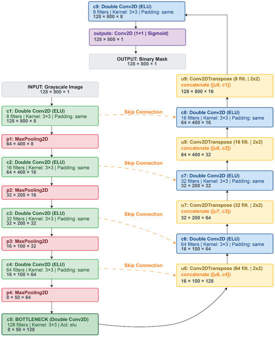
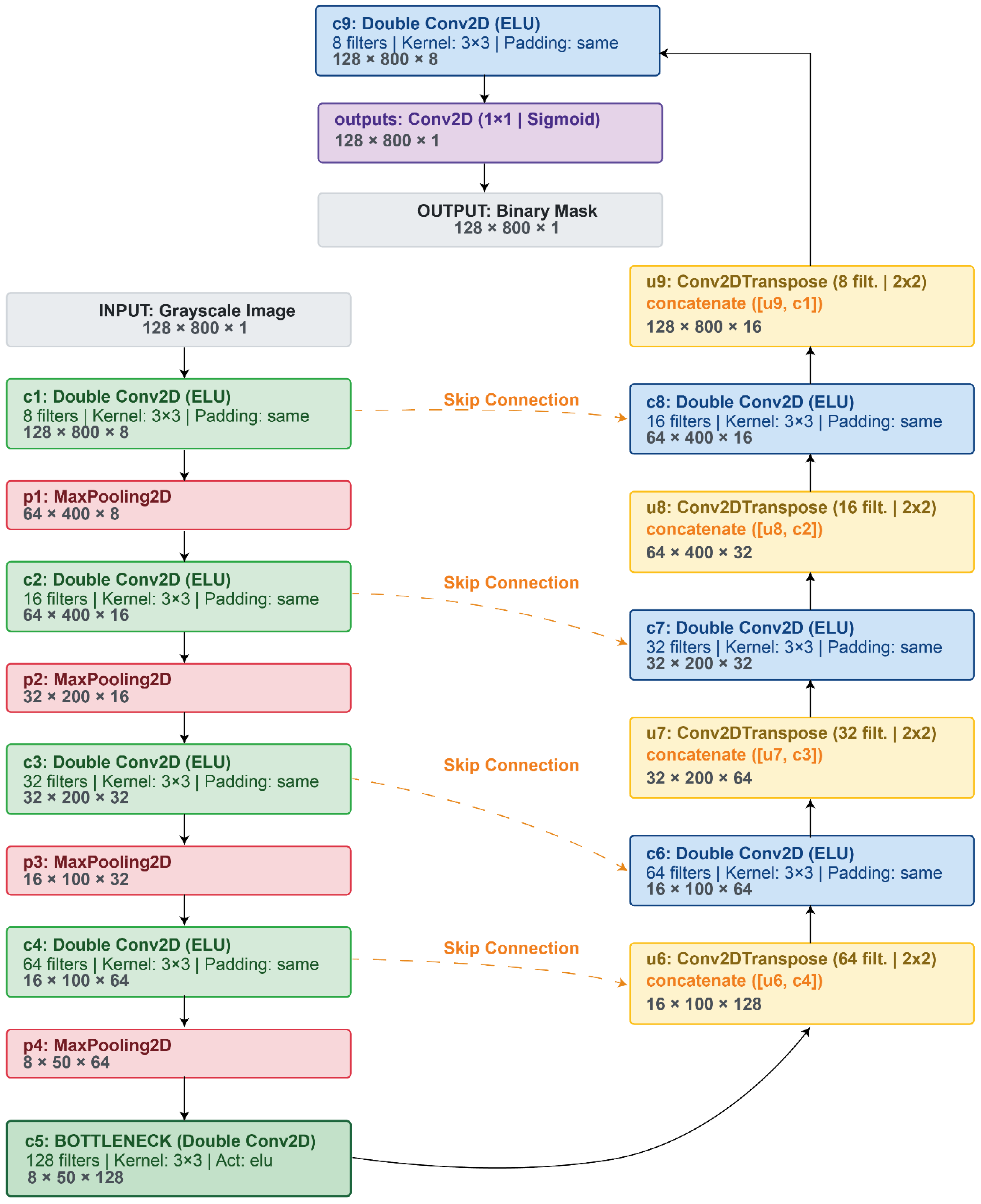
The segmentation model implements the U-Net architecture [7], originally developed for biomedical image segmentation and subsequently applied across numerous industrial inspection tasks. The architecture follows a symmetric encoder–decoder structure. The encoder path applies successive convolutional blocks interleaved with max-pooling operations to progressively extract feature representations at increasing levels of abstraction. The decoder path applies transposed convolution operations to recover spatial resolution, receiving skip connections from the corresponding encoder levels that preserve fine-grained spatial information. The architecture employed is depicted in Figure 1.

Figure 1. U-Net architecture employed in the experiment. The encoder path (left) applies successive convolutional blocks with max-pooling to extract hierarchical features. The bottleneck (center-bottom) captures the most abstract representation. The decoder path (right) recovers spatial resolution via transposed convolutions. Skip connections concatenate encoder feature maps to their corresponding decoder levels, preserving the spatial detail essential for accurate defect boundary delineation. The final 1 × 1 convolution with sigmoid activation produces the binary segmentation mask. Loss function: combined BCE + Dice Loss.

The final layer applies a 1 × 1 convolution producing a binary output mask, with sigmoid activation, corresponding to the defect and background classes. The architecture is well suited for tasks characterized by limited labeled data and irregular boundary morphology, both of which are prominent features of steel surface defect datasets [11].

3.4. Training Configuration

Training was conducted for a maximum of 2000 epochs with the Adam optimizer (initial learning rate 1 × 10⁻⁴) and a batch size of 32. The loss function combined Binary Cross-Entropy (BCE) and Dice Loss in an equally weighted (unweighted) sum, L = BCE + (1 − Dice), as expressed in Equation (1):

L = α · L_BCE + β · (1 − L_Dice)

(1)

where L_BCE is the standard binary cross-entropy term and L_Dice is the Dice coefficient measuring overlap between the predicted and ground-truth masks, α = β = 1. The combined loss addresses the class imbalance inherent in the dataset: the BCE component promotes the correct pixel-level classification, while the Dice component optimizes the spatial overlap between predicted and reference segmentation regions. Three training callbacks were employed: EarlyStopping, which terminates training when validation loss does not improve over a specified patience window; ModelCheckpoint, which saves the model state corresponding to the best validation loss; and ReduceLROnPlateau, which reduces the learning rate when the validation loss plateaus, preventing oscillation around local minima.

3.5. Hardware and Software Environment

Experiments were conducted on a dedicated workstation equipped with an NVIDIA GeForce RTX 3060 GPU (Samsung Electronics, Pyeongtaek Campus Godeok-myeon, Pyeongtaek-si, Gyeonggi-do, Republic of Korea) with 12 GB of GDDR6 memory. The deep learning framework was Keras with a TensorFlow 2.10 backend, running within a GPU-accelerated Python 3.9 environment. The trained U-Net has 485,673 parameters, corresponding to a checkpoint of approximately 1.85 MB in FP32 (0.93 MB in FP16). The hardware environment is detailed in Table 1.

3.6. Evaluation Metrics

Model performance was evaluated with region-overlap and pixel-classification metrics computed against the ground-truth masks: the Dice coefficient (equivalently F1 for binary segmentation), Intersection over Union (IoU), pixel-level precision and recall, and pixel accuracy. Because the dataset is dominated by background pixels, pixel accuracy is reported only alongside a trivial all-background baseline and is not used as the primary metric; Dice, IoU, precision, recall, and F1 are the primary metrics, each accompanied by a 95% confidence interval obtained by a non-parametric bootstrap (10,000 resamples over the test images). A precision–recall curve obtained by sweeping the decision threshold, and metrics stratified by defect class and by defect area are also reported. Inference time per image was measured to assess real-time deployment feasibility.

4. Results

4.1. Training Behavior

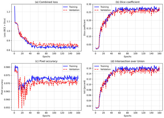
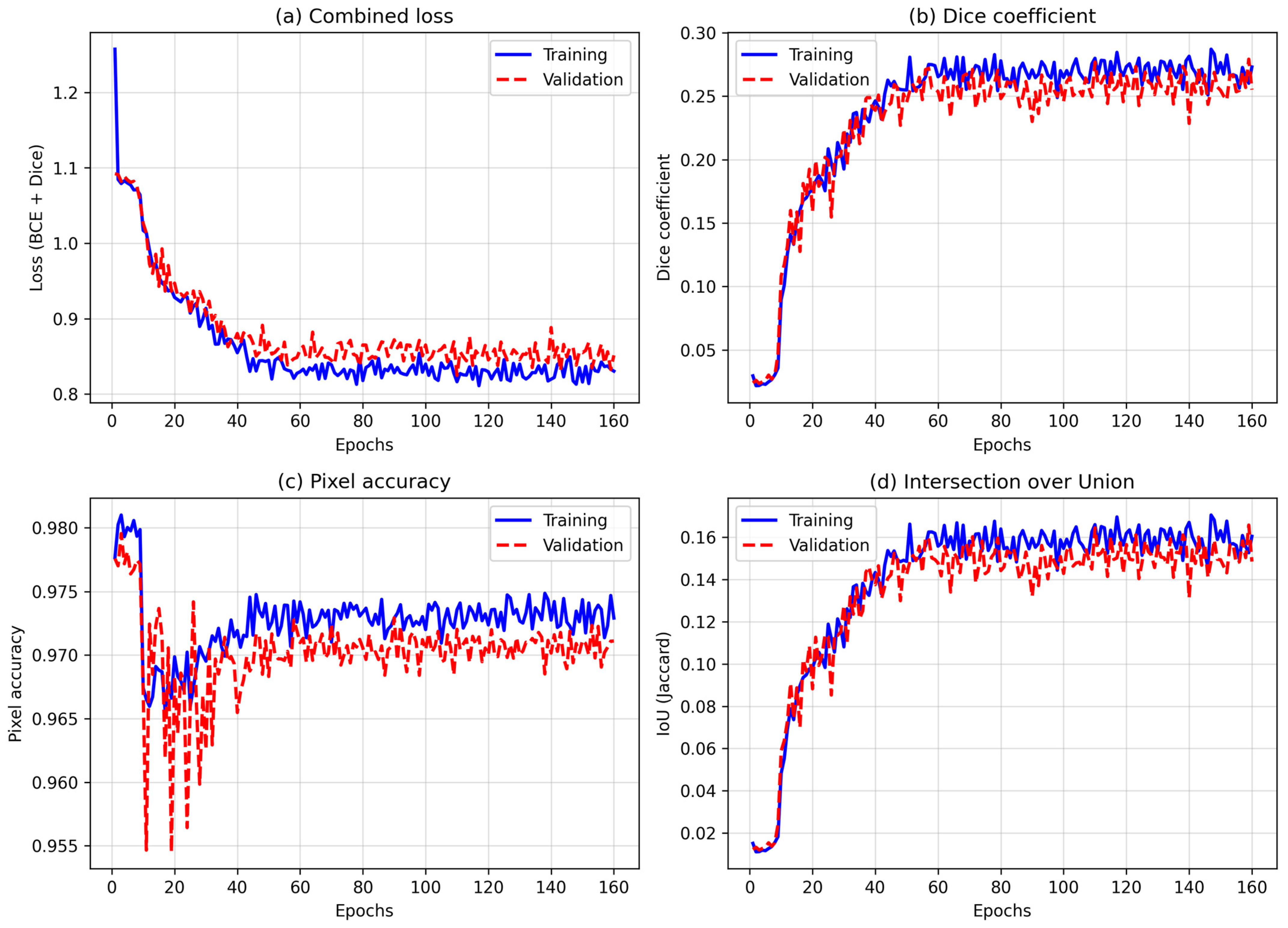
Training was terminated by the EarlyStopping callback after 160 epochs, at which point the validation loss ceased to decrease; the ModelCheckpoint callback preserved the best-validation weights and ReduceLROnPlateau lowered the learning rate at stagnation points, contributing to a smooth convergence profile. The training dynamics are summarized in the consolidated panel of Figure 2, presenting the combined loss, the Dice coefficient, the pixel accuracy, and the IoU across the training and validation partitions.

Figure 2. Training dynamics on the clean split, shown as a consolidated panel: (a) combined BCE+Dice loss, (b) Dice coefficient, (c) pixel accuracy, and (d) IoU, for the training (solid) and validation (dashed) partitions.

On the clean stratified split, the combined loss declined consistently on both the training and validation partitions and stabilized at approximately 0.83. The soft (un-thresholded) Dice coefficient and IoU recorded during training stabilized at approximately 0.27 and 0.16, respectively, with the validation trajectories closely tracking their training counterparts, indicating generalization without significant overfitting. These soft training values are lower than the thresholded test-set Dice reported in Section 4.2, and their moderate magnitude is consistent with the severe class imbalance of the dataset.

While the primary experimental evaluation focuses on segmentation precision and processing speed, the practical translation of these metrics into plant-level outcomes—such as First Pass Yield (FPY) and False Escape Rate—is detailed in Appendix A.

4.2. Test-Set Performance

On the leakage-free test set of 1886 images, the compact from-scratch U-Net attains a Dice coefficient of 0.416 (95% CI 0.393 to 0.439), an IoU of 0.263, a precision value of 0.387, a recall score of 0.451, and a pixel accuracy of 95.77%. Crucially, a trivial predictor that labels every pixel as background reaches a higher pixel accuracy of 96.66% while scoring 0 on Dice, IoU, precision, and recall; this demonstrates that pixel accuracy is not an informative metric on this heavily imbalanced dataset and motivates the overlap-based metrics used throughout. A DeepLabV3+ (ResNet-50) model trained on the identical split reaches a substantially higher Dice of 0.677 (95% CI 0.660 to 0.695), and a classical Otsu baseline reaches only 0.060, bracketing the U-Net between a strong pretrained baseline and a classical lower bound. All test-set metrics, each with a 95% bootstrap confidence interval, are summarized in Table 2.

Table 2. Test-set performance on the clean, leakage-free split (1886 images). Dice and IoU are shown with 95% bootstrap confidence intervals. Params = trainable parameters; latency = mean inference time per image on the RTX 3060.

Model	Dice	IoU	Precision	Recall	F1	Pixel Acc.	Params	Latency
Trivial (all-background)	0.000	0.000	0.000	0.000	0.000	0.967	-	-
Otsu + morphology	0.060 [0.054–0.066]	0.031	0.033	0.306	0.060	0.678	-	-
U-Net (from scratch)	0.416 [0.393–0.439]	0.263 [0.244–0.281]	0.387	0.451	0.416	0.958	485,673	38.6 ms
DeepLabV3+ (ResNet-50)	0.677 [0.660–0.695]	0.512 [0.492–0.532]	0.602	0.774	0.677	0.975	17,830,209	46.3 ms

Baseline Comparison, Per-Class and Per-Area Analysis

Two reference points frame the U-Net result. A classical pipeline (Otsu thresholding followed by morphological opening/closing and small-component removal) reaches a Dice of only 0.060, confirming that the task is not solvable by intensity thresholding. Conversely, a DeepLabV3+ model with an ImageNet-pretrained ResNet-50 encoder, trained on the identical split with the same loss and protocol, reaches a Dice of 0.677 at the cost of 37 times more parameters (17.8 M vs. 0.49 M) and higher latency (46.3 ms vs. 38.6 ms). The compact U-Net therefore trades absolute accuracy for a far smaller, edge-friendlier footprint. The per-class results (Table 3) show that both models perform best on the dominant class 3 and struggle on the rare class 2 (33 test images); the pretrained DeepLabV3+ model recovers this class markedly better (Dice 0.27 vs. 0.03). Stratifying by defect area (Table 4) quantifies the effect of the 128 × 800 downsampling: for both models the Dice increases monotonically with defect size, while recall stays comparatively high even for the smallest defects, indicating that downsampling primarily erodes boundary precision rather than the detection of fine defects.

Table 3. Dice coefficient by original defect class (ClassId 1 to 4), where multi-class images or defect-free images (background-only) are disregarded.

ClassId	Test Images	U-Net Dice	DeepLabV3+ Dice
1	132	0.415	0.504
2	33	0.033	0.268
3	778	0.518	0.701
4	120	0.421	0.649

Table 4. Dice coefficient by defect-area quartile (mask area in pixels).

Quartile	Area (px at 128 × 800)	Test Images	U-Net Dice	DeepLabV3+ Dice
Q1	67–1113	250	0.334	0.475
Q2	1113–2684	250	0.460	0.611
Q3	2692–7267	250	0.489	0.630
Q4	7315–73,185	250	0.520	0.722

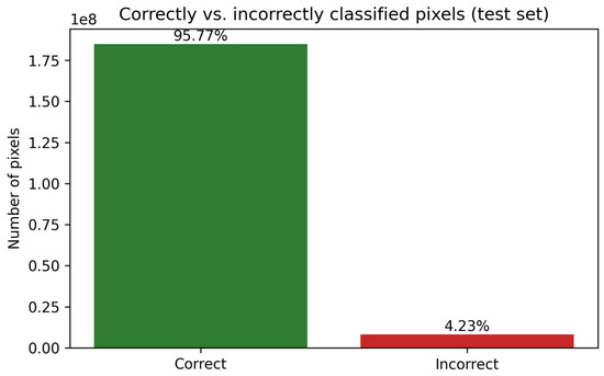
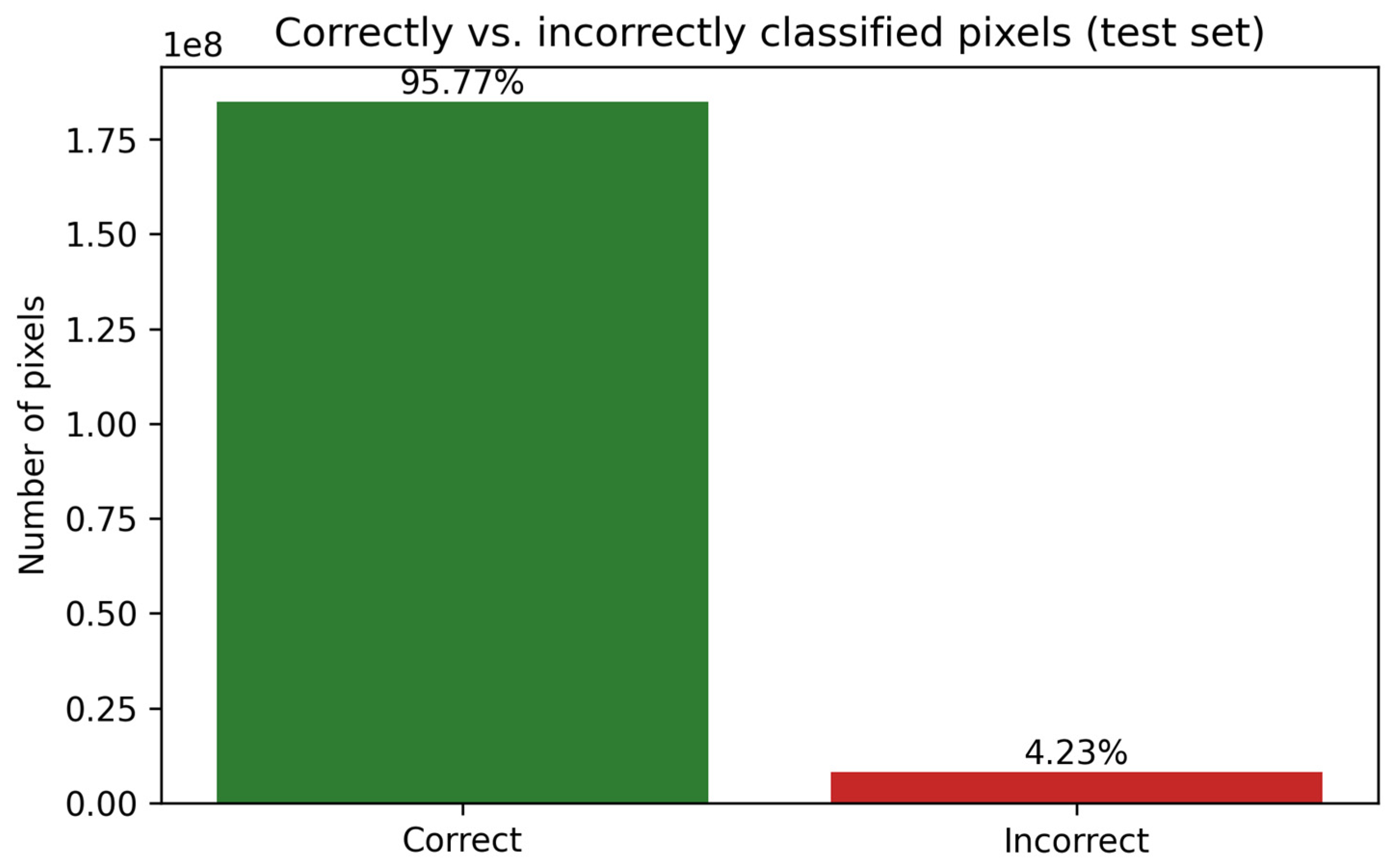
Crucially, a trivial predictor that labels every pixel as background reaches a higher pixel accuracy of 96.66% while scoring 0 on Dice, IoU, precision, and recall. The U-Net’s pixel accuracy of 95.77% is marginally lower than the trivial baseline because the model deliberately over-segments defect boundaries to maximize recall, a trade-off governed by the combined loss function that prioritizes reducing false escapes over minor boundary expansion. This confirms that pixel accuracy is a misleading metric for highly imbalanced segmentation datasets and reinforces overlap-based metrics as the true performance benchmark.

4.3. Per-Sample Analysis

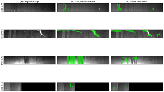
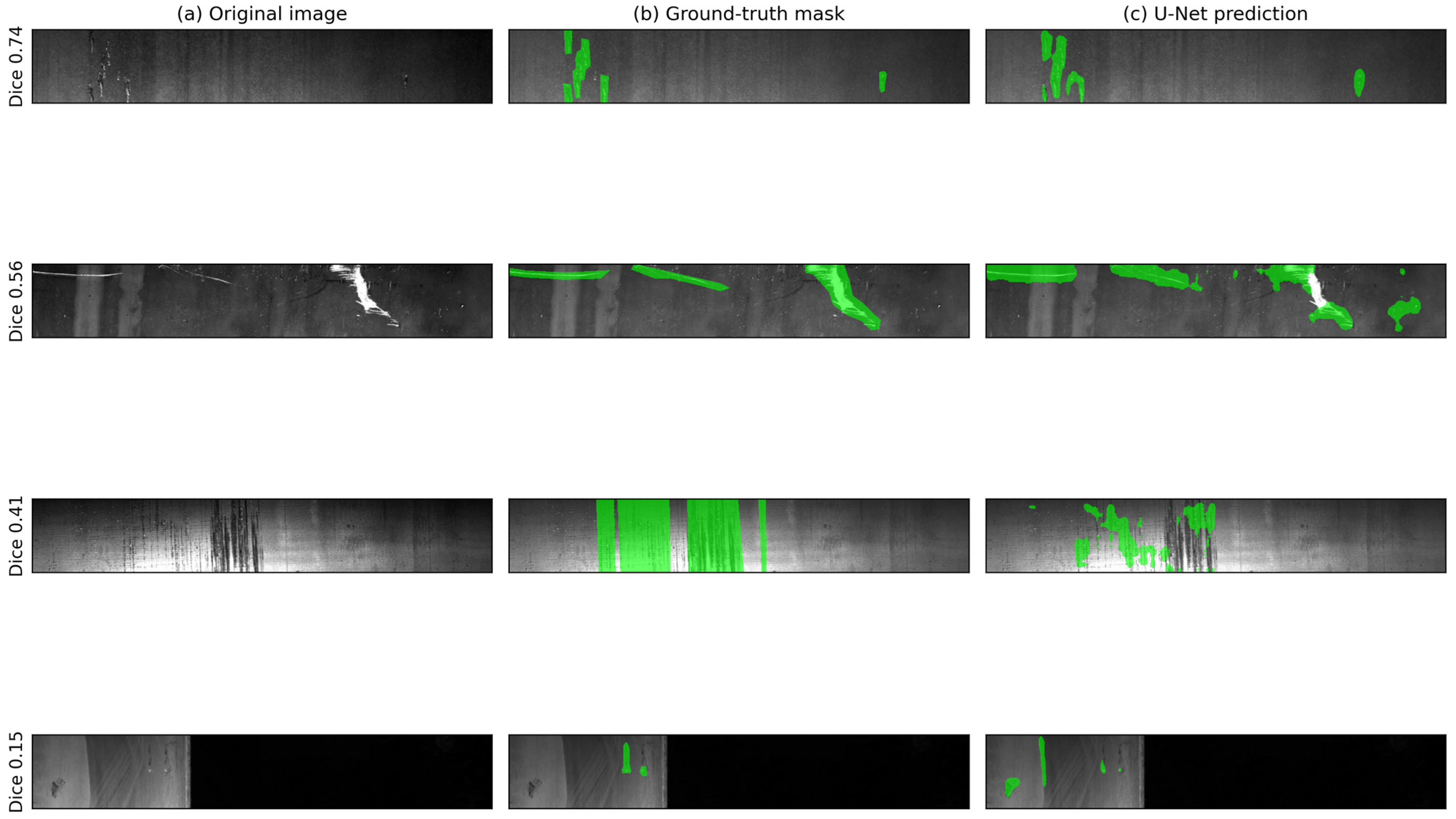
A qualitative examination of individual test predictions is shown in Figure 3, which presents four representative cases from the clean test set, ordered from the highest to the lowest Dice, each as (a) the original grayscale image, (b) the ground-truth mask, and (c) the U-Net prediction.

Figure 3. Representative U-Net segmentation results on the clean test set, ordered by Dice from top (best) to bottom (worst): (a) original grayscale line-scan image, (b) ground-truth binary mask, (c) U-Net prediction. Green overlays mark defect pixels.

In the highest-Dice case (top row), a linear surface discontinuity with well-defined contrast is accurately localized, with only minor boundary dilation. This slight over-segmentation at boundaries is characteristic of models trained with a combined BCE and Dice loss and is operationally acceptable, since a marginally wider alert zone around a true defect is preferable to a missed detection.

In the intermediate cases (middle rows), defects under elevated illumination, reflections, or scale deposits are still localized, but the model occasionally segments adjacent surface irregularities, such as scale particles, that resemble true defects; the segmented regions nonetheless remain spatially proximate to the actual defect areas.

In the lowest-Dice case (bottom row), fine or fragmented defects are only partially recovered, and the predicted mask is broader than the reference, consistent with the loss of boundary precision quantified per defect-area quartile in Table 4.

The overall distribution of correctly versus incorrectly classified pixels across the full 1886-image test set is shown in Figure 4, consolidating the per-image behavior into a single batch-level view.

Figure 4. Distribution of correctly versus incorrectly classified pixels over the full 1886-image test set. Because defect-free background dominates, a high pixel-accuracy value coexists with a modest Dice, underscoring why overlap-based metrics are used as the primary measures.

4.4. Inference Latency

Averaged over the 1886-image test set, the U-Net has a mean inference time of 38.6 ms per image on the RTX 3060, measured image-by-image (the DeepLabV3+ baseline requires 46.3 ms); under batched execution, the effective throughput corresponds to approximately 22.7 ms per image. This latency was measured without hardware-specific optimization such as TensorRT quantization or ONNX export. Production deployment on a dedicated edge inference device would further reduce latency through model quantization and hardware-specific optimization; the NVIDIA Jetson family of embedded GPU modules, for instance, offers throughput consistent with or exceeding the latencies observed here for segmentation workloads of comparable scale [20].

4.5. Robustness to Synthetic Perturbations

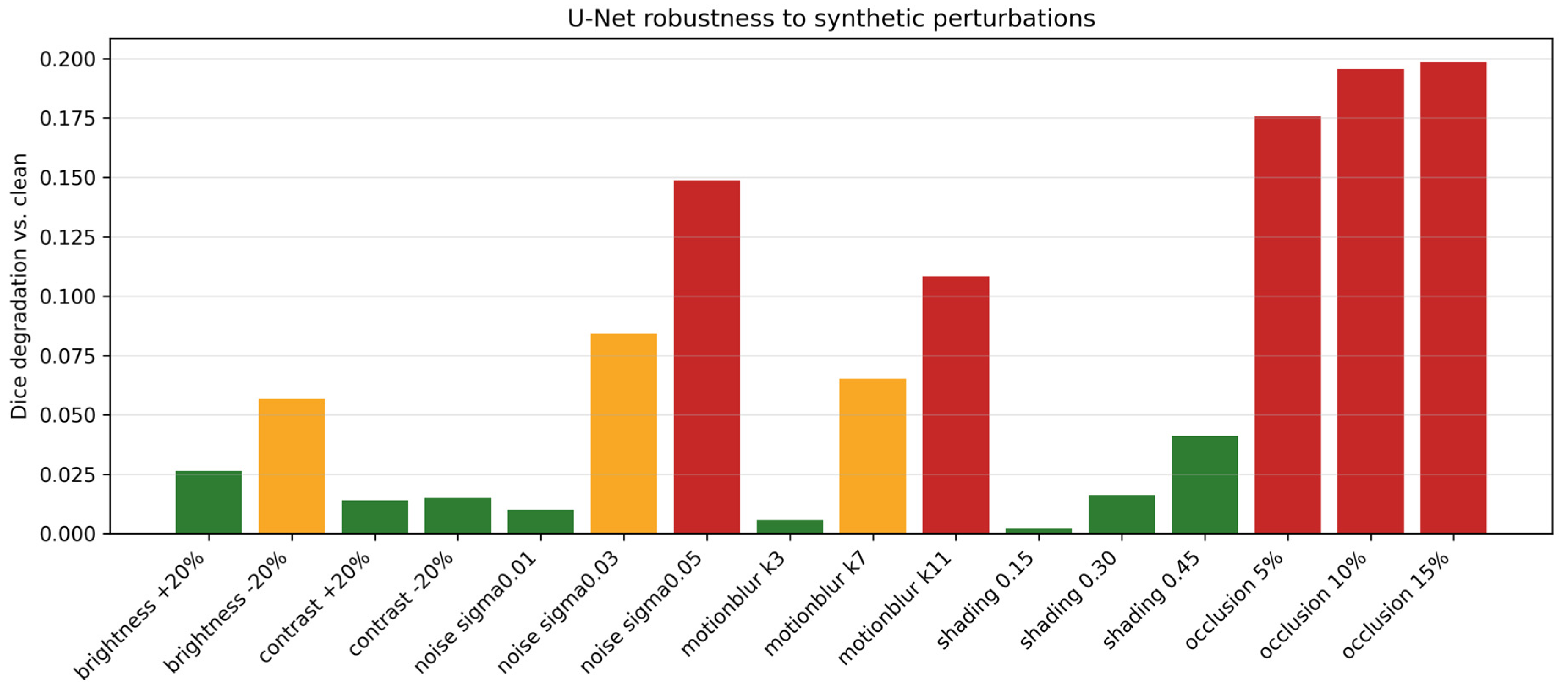
To probe robustness under realistic acquisition disturbances, the clean test set was perturbed (without retraining) and re-evaluated with the best U-Net checkpoint. Rectangular occlusion was the most damaging factor (with a Dice drop of up to 0.199 at 15% coverage), followed by sensor noise (0.149 at sigma = 0.05) and horizontal motion blur (0.108 at an 11-pixel kernel). Illumination shifts were comparatively mild but asymmetric: darkening (−20% brightness) degraded the Dice about twice as much as brightening (0.057 vs. 0.026). Low-frequency shading and small amounts of noise or blur had a negligible effect. These findings translate into concrete deployment priorities: guarding the optical path against occlusion and contamination, stabilizing illumination against darkening, and controlling vibration. They are summarized in Table 5 and Figure 5.

Table 5. U-Net Dice under synthetic perturbations (clean-test Dice = 0.416); drop is relative to the clean value.

Perturbation	Dice	IoU	Recall	Dice Drop
Brightness +20%	0.390	0.242	0.368	0.026
Brightness −20%	0.360	0.219	0.352	0.057
Contrast +20%	0.402	0.252	0.461	0.014
Contrast −20%	0.401	0.251	0.401	0.015
Noise sigma = 0.01	0.406	0.255	0.419	0.010
Noise sigma = 0.03	0.332	0.199	0.300	0.084
Noise sigma = 0.05	0.267	0.154	0.214	0.149
Motion blur k = 3	0.411	0.258	0.403	0.006
Motion blur k = 7	0.351	0.213	0.295	0.065
Motion blur k = 11	0.308	0.182	0.231	0.108
Shading 0.15	0.414	0.261	0.457	0.002
Shading 0.30	0.400	0.250	0.465	0.016
Shading 0.45	0.375	0.231	0.476	0.041
Occlusion 5%	0.241	0.137	0.448	0.176
Occlusion 10%	0.221	0.124	0.404	0.196
Occlusion 15%	0.218	0.122	0.367	0.199

Figure 5. U-Net Dice degradation under synthetic perturbations, relative to the clean test set. Occlusion and higher-intensity sensor noise are the most damaging; darkening degrades the model roughly twice as much as brightening.

5. Proposed IIoT Architecture

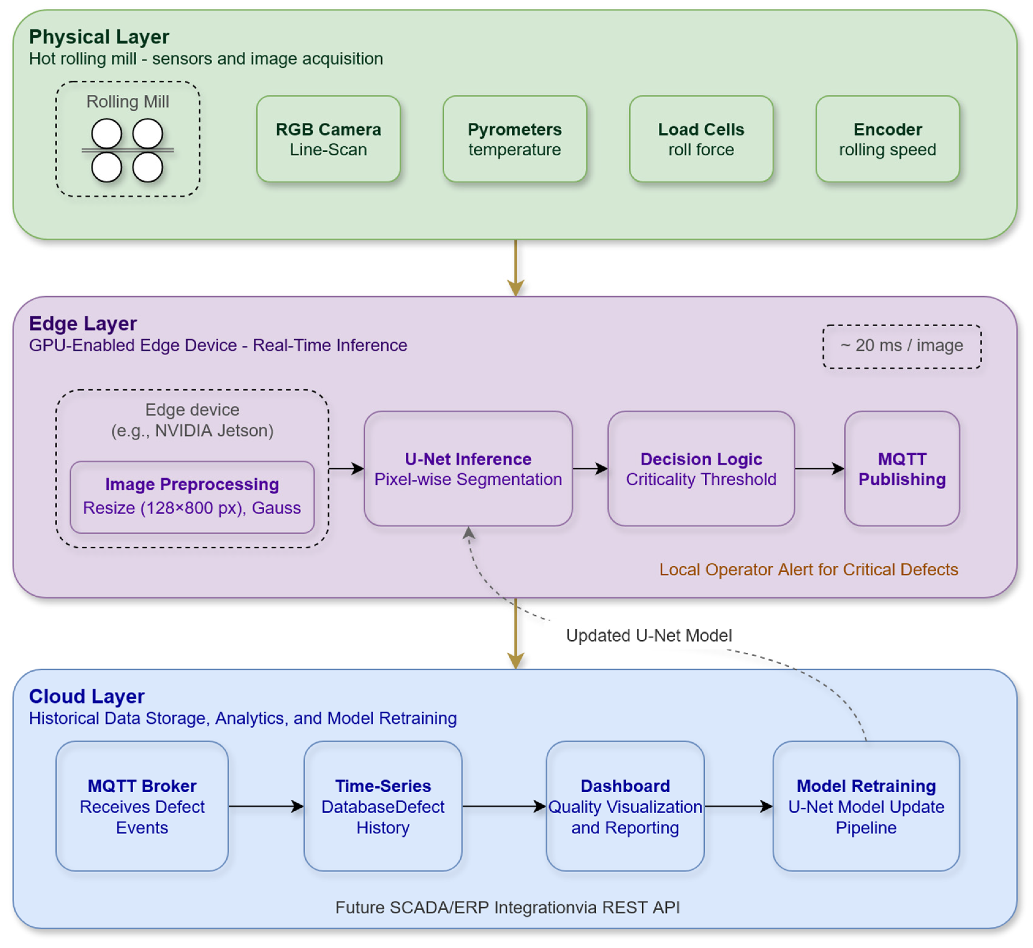
The proposed architecture is motivated by a central requirement derived from the experimental results reported in Section 4: the trained U-Net model achieves a mean inference time of approximately 22.7 ms per image under conventional GPU conditions, a latency budget that is compatible with real-time feedback in production environments when deployed on dedicated edge hardware. The architecture does not represent a currently implemented system; rather, it constitutes a conceptual design framework, grounded in established IIoT layering principles, that serves as the target for future physical implementation. The overall structure is illustrated in Figure 6.

Figure 6. Proposed three-layer IIoT architecture for real-time steel surface defect detection. The Physical Layer captures images and process data from the rolling line. The Edge Layer runs U-Net inference locally (~23 ms/image) and publishes results via MQTT. The Cloud Layer stores historical defect data, provides dashboards, and supports periodic model retraining. The dashed arrow indicates the model update feedback path.

The architecture is organized in three layers, following the structural pattern established in the IIoT literature [6]: a Physical/Sensing Layer, an Edge Computing Layer, and a Cloud Analytics Layer. The three layers communicate via standardized industrial protocols, with MQTT as the primary messaging protocol between edge and cloud, in alignment with its widely documented suitability for low-overhead IIoT messaging [21].

5.1. Physical Layer

The Physical Layer comprises the instrumentation deployed directly on or adjacent to the steel rolling line. High-resolution RGB cameras, positioned along the production line at points determined by process requirements, capture images of the steel surface during active rolling. Additional sensors, including pyrometers for temperature monitoring, load cells for roller force measurement, encoders for speed and position tracking, and ultrasonic or LIDAR sensors for thickness and flatness measurement, provide complementary process data that can be correlated with detected defects for root-cause analysis.

The physical environment of a hot rolling mill presents substantial instrumentation challenges: high temperatures, cooling water, poor ambient lighting, mechanical vibrations, and contamination from scale and lubrication all affect sensor reliability. The architecture assumes hardened industrial-grade cameras with protective enclosures and synchronized illumination, consistent with commercial surface inspection systems currently deployed in the industry.

5.2. Edge Computing Layer

The Edge Computing Layer is the core computational node of the proposed architecture. An embedded GPU device, such as the NVIDIA Jetson family of modules, receives the image stream from the Physical Layer cameras and executes the trained U-Net model in real time. The latency measured in this study on the reference workstation GPU, reported in Section 4.4, characterizes the computational cost of the network itself and provides an upper-bound reference for embedded execution. Measured latency, memory occupancy, power consumption, and throughput on embedded hardware have not been obtained in the present study, and their determination is identified as the primary immediate next step (Section 6).

The edge node implements the following pipeline: (1) image acquisition and pre-processing, including resizing to the model input resolution of 128 × 800 pixels and Gaussian noise filtering; (2) U-Net inference producing a binary segmentation mask; (3) defect decision logic, applying a threshold to determine whether the current image exceeds a criticality criterion; and (4) result publication via MQTT to the cloud broker. If a defect above the threshold is detected, an immediate local alert can be issued to the production line operator, enabling corrective action before additional material is processed.

The separation of inference from training, with training performed in the cloud and inference deployed at the edge, follows established cloud–edge collaboration paradigms for IIoT deployments. This separation avoids the latency and bandwidth costs of transmitting raw images to the cloud for every frame, while retaining the benefits of centralized model development and retraining.

5.3. Cloud Analytics Layer

The cloud analytics layer receives structured inference results, rather than raw images, from the edge node via the MQTT protocol. This layer is responsible for historical storage of defect events, correlated with process metadata; visualization through operator dashboards; generation of statistical quality reports; and periodic retraining of the U-Net model as new labeled defect data accumulates.

The architecture envisions integration with existing industrial systems, including SCADA and ERP platforms, through standard web service interfaces, consistent with the integration approach documented in the steel casting monitoring system of Zhang et al. [6]. This integration would allow defect events to automatically generate maintenance notifications, production grade flags, or material traceability records without manual data re-entry. The components, communication protocols, and primary function of each layer are summarized in Table 6.

Table 6. Summary of the proposed three-layer IIoT architecture components, communication protocols, and functions.

Layer	Key Components	Protocols/ Standards	Primary Function
Physical Layer	RGB line-scan cameras, pyrometers, load cells, encoders	Analog/digital I/O, CAN bus	Acquire high-resolution surface images and process variables (temperature, force, speed) continuously during rolling
Edge Computing Layer	Embedded GPU device (e.g., NVIDIA Jetson), trained U-Net model, decision logic module	MQTT (publish), local alert I/O	Execute U-Net inference locally (~23 ms/image); apply defect criticality threshold; issue real-time operator alerts; publish structured results to cloud broker
Cloud Analytics Layer	MQTT broker, time-series database, visualization dashboard, U-Net retraining pipeline	MQTT (subscribe), REST API, SCADA/ERP integration (future)	Store historical defect events correlated with process metadata; provide quality dashboards and statistical reports; retrain and redeploy U-Net model as new labeled data accumulates

5.4. Deployment Considerations and Edge Platform Selection

This inference performance is directly relevant to the IIoT architecture developed in this section. The two execution regimes must be distinguished. Image-by-image execution, which is the regime relevant to per-frame alert generation, yields 38.6 ms per image, equivalent to 25.9 frames per second and therefore below the 30 to 50 fps typical of industrial line-scan acquisition. Batched execution reaches an effective 22.7 ms per image, equivalent to 44 frames per second, but introduces a queueing delay proportional to the batch size and is therefore appropriate for buffered analysis rather than for immediate alerting. Closing this gap in the per-frame regime requires hardware-specific optimization such as TensorRT compilation or reduced-precision inference, which has not been performed in this study. These figures characterize the computational cost of the network on the reference workstation GPU and provide an upper-bound reference for embedded deployment; measured latency, memory occupancy, and power consumption on embedded hardware have not been obtained in this study and are identified as the primary immediate next step (Section 6). This interpretation is consistent with recent IIoT research on time-sensitive industrial networks, where machine learning-based runtime decision logic is integrated with real-time monitoring to support proactive fault responses under latency-constrained conditions [22].

Human visual inspection, by contrast, operates under fundamentally different latency and availability constraints: it requires the production line to be stopped or the steel to be cooled before sample examination, introduces subjective variability between inspectors, and has documented detection reliability limitations. The 22.7 ms inference result demonstrates that deep learning-based inspection can address all three of these limitations simultaneously.

Table 7 provides a structured comparison of five representative edge hardware platforms against seven deployment dimensions relevant to IIoT integration of deep learning-based inspection systems. The assessment is qualitative, grounded in published hardware specifications and documented industrial deployments [20,23,24,25], and is intended as a practical reference for implementers planning the physical deployment of architectures similar to the one proposed in this section.

Table 7. Comparative assessment of edge hardware platforms for IIoT-integrated deep learning inspection. Qualitative ratings (Very high/High/Medium/Low/Very low) are derived exclusively from published hardware specifications and documented industrial deployments [20,23,24,25]. No entry of this table was measured in the present study; the only platform characterized experimentally here is the Raspberry Pi, operating in the role of message broker rather than of inference node (Section 5.5). The table therefore supports platform pre-selection and does not substitute for the embedded benchmarking identified as the immediate next step. DL = deep learning; INT8 = 8-bit integer quantization; OTA = over-the-air update.

Platform	DL Inference Latency	Industrial Ruggedness	IIoT Protocol Support	DL Framework Support	Energy Consumption	Deployment Complexity	Lifecycle/Support
NVIDIA Jetson Orin NX	High—GPU-accelerated TensorRT; <10 ms with INT8	Medium—requires enclosure for harsh environments	MQTT, OPC UA, REST; CUDA-native	TensorFlow, PyTorch, ONNX, TensorRT	Medium (10–25 W)	Medium—SDK setup, OTA update supported	High—NVIDIA long-term support roadmap
NVIDIA Jetson Nano	Medium—GPU inference; 20–40 ms for U-Net at 128 × 800	Medium—requires enclosure for harsh environments	MQTT, REST; CUDA-native	TensorFlow, PyTorch, ONNX; limited TensorRT	Low (5–10 W)	Low—broad community support, documented	Medium—legacy module, limited new development
Raspberry Pi 5	Low—CPU-only; >200 ms for U-Net without accelerator	Low—consumer-grade; sensitive to vibration and heat	MQTT, REST, OPC UA via libraries	TensorFlow Lite, ONNX Runtime; no native GPU	Very low (<5 W)	Very low—widely documented, rapid prototyping	Medium—community-driven, uncertain industrial lifecycle
Google Coral Dev Board	High—Edge TPU; <5 ms for INT8 quantized models	Medium—requires enclosure; limited temperature range	MQTT, REST via host SoC	TensorFlow Lite (INT8 only); limited model flexibility	Very low (2–4 W)	Medium—requires INT8 quantization pipeline	Low—Coral lifecycle uncertain post-2023
Industrial FPGA (e.g., Intel Arria/Xilinx Zynq)	Very high—deterministic <5 ms; hardware pipeline	High—industrial-grade variants rated for harsh environments	OPC UA, PROFINET, EtherCAT, MQTT via soft-IP	Custom IP cores; high engineering effort for DL	Low–Medium (5–20 W depending on design)	High—specialized HDL expertise required	Very high—long industrial lifecycle, IEC certifiable

The comparison in Table 7 reveals a fundamental trade-off that practitioners must navigate: the platforms offering the highest inference performance and industrial lifecycle assurance (FPGA, Jetson Orin NX) impose the greatest deployment complexity and engineering effort, while the platforms that minimize deployment friction (Raspberry Pi 5) are inadequate for low-latency inference of U-Net-scale models without external accelerators. For the architecture proposed in this section, the NVIDIA Jetson Orin NX represents the most technically aligned choice, offering sub-10 ms inferences with TensorRT optimization, native MQTT support, and a documented industrial deployment trajectory. The Jetson Nano remains viable for pilot implementations where latency constraints are relaxed, and hardware budgets are limited. Industrial FPGA platforms become compelling when deterministic latency, a long asset lifecycle exceeding ten years, and integration with fieldbus protocols such as PROFINET or EtherCAT are requirements imposed by the plant environment. The relevant distinction regarding quantization is not whether INT8 is supported but whether it is optional or mandatory. On Jetson-class platforms, INT8 is an optimization option available through TensorRT alongside FP16 and FP32, and it can be bypassed when accuracy does not tolerate it. On Google Coral, by contrast, the Edge TPU operates exclusively in 8-bit integer arithmetic, so quantization is a hardware constraint with no floating-point fallback. The Coral is therefore appropriate only where the accuracy loss associated with mandatory quantization is acceptable; for fine-grained steel defects that loss should be measured before deployment, and the uncertain product lifecycle is a further consideration. Framed in this way the assessment is a design trade-off rather than a categorical exclusion.

5.5. Experimental Validation of the Messaging Layer

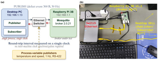
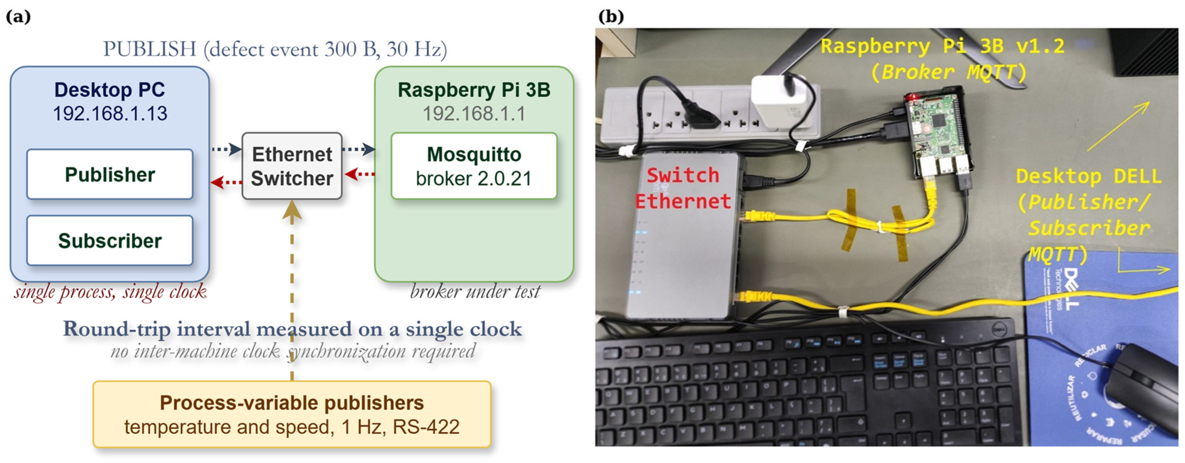
The messaging layer of the proposed architecture was implemented at laboratory scale and characterized under a continuous load. The bench consists of a Mosquitto broker (version 2.0.21) hosted on a Raspberry Pi 3 Model B, connected through a dedicated Ethernet switch to a desktop host that publishes structured defect events at 30 Hz. Each event is encoded as a JSON payload of approximately 300 bytes containing the image identifier, defect area, defect fraction, maximum confidence score, inference time, and criticality flag, representing the output that the inference node of Section 5.2 would produce at deployment. The publisher and subscriber execute in the same process on the same host, so that publication and reception instants are read from a single clock and no inter-machine clock synchronization is required; the measured interval therefore corresponds to the complete round trip through the switch and the broker. Two additional publishers emit simulated process variables through RS-422 serial interfaces, representing the pyrometer and encoder streams of the Physical Layer described in Section 5.1. Both hosts communicate exclusively over the wired link, with wireless interfaces disabled, and the power management of the Ethernet adapter on the desktop host was disabled, for the reasons reported in Section 5.5.1. The junction temperature of the broker host was recorded before and after every run and remained between 53 and 55 degrees Celsius, with the thermal throttling status confirmed as inactive throughout, so that no measurement was affected by processor frequency reduction. The bench is shown in Figure 7.

Figure 7. Laboratory bench used to characterize the messaging layer. (a) Measurement topology: the publisher and subscriber execute in the same process on the desktop host, so that publication and reception instants are read from a single clock, while the Mosquitto broker under test runs on the Raspberry Pi. (b) Physical implementation of the bench.

5.5.1. Effect of the Host and Transport Configuration

An initial characterization produced a counter-intuitive ordering: the quality-of-service level without delivery guarantee was an order of magnitude slower than the level with acknowledgment. The cause was traced to the interaction between the Nagle algorithm, which withholds small segments until previous data is acknowledged, and the delayed acknowledgment mechanism of TCP. Under QoS 1, the returning PUBACK packets keep the connection active and the effect is masked; under QoS 0, there is no return traffic, and small payloads accumulate in the transmission buffer.

Because a publish–subscribe chain comprises two independent transport legs, publisher to broker and broker to subscriber, a full factorial experiment was conducted in which the Nagle algorithm was enabled or disabled at each end. The four configurations were evaluated at 30 Hz with 1800 messages per run and the three quality-of-service levels. Table 8 reports the results.

Table 8. Median latency, with the 99th percentile in parentheses, for the four transport configurations. Values are in milliseconds, with 1800 messages per run at 30 Hz.

Config.	Broker Socket	Client Socket	QoS 0	QoS 1	QoS 2
A	Nagle	Nagle	33.09 (58.4)	1.83 (2.9)	4.35 (5.9)
B	Nagle	TCP_NODELAY	31.03 (61.0)	1.69 (2.5)	22.60 (39.9)
C	TCP_NODELAY	Nagle	1.88 (2.7)	1.74 (2.7)	3.76 (5.1)
D	TCP_NODELAY	TCP_NODELAY	1.92 (2.8)	1.78 (2.5)	4.25 (5.7)

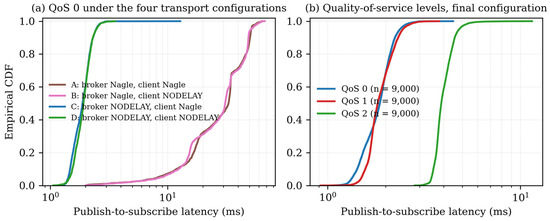
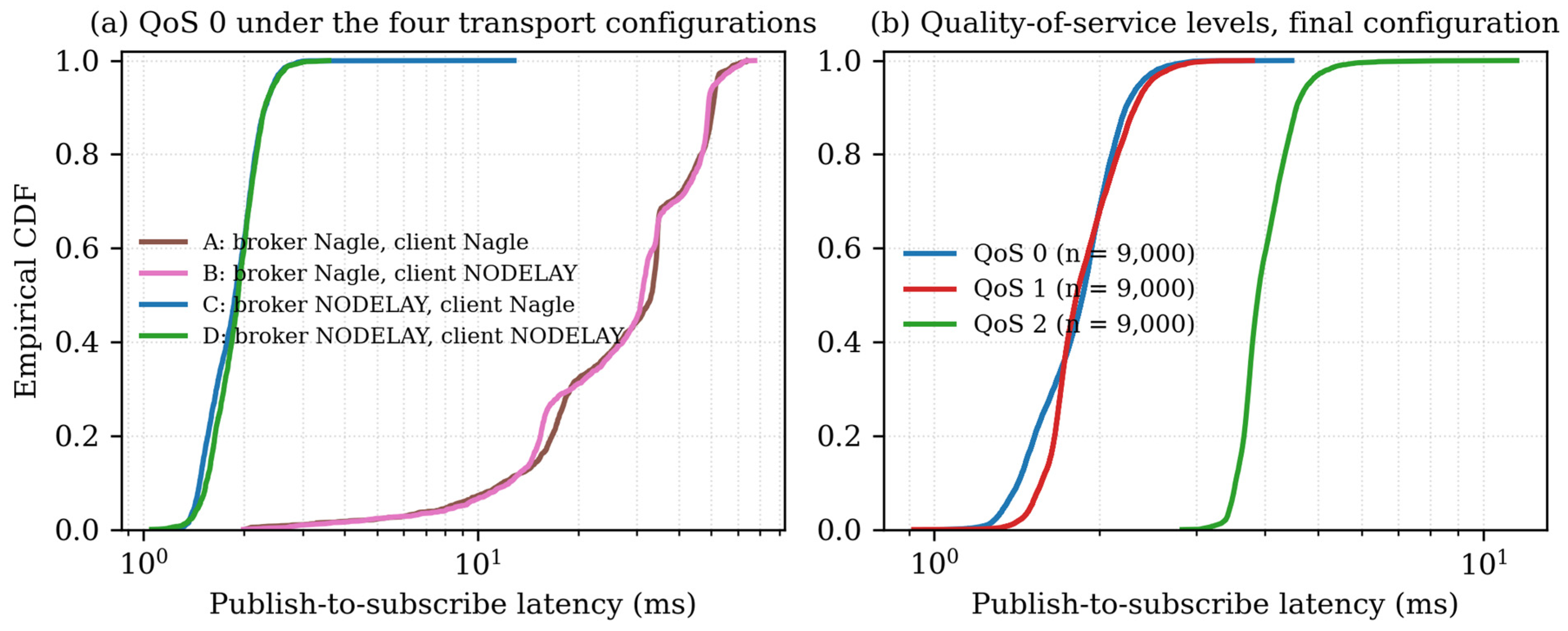
The outcome is unambiguous and, to the best of our knowledge, has not been reported for MQTT deployments in an industrial monitoring context. Disabling the Nagle algorithm at the publisher alone produces no meaningful improvement, from 33.09 ms to 31.03 ms, whereas disabling it at the broker reduces the median latency to 1.88 ms, a factor of seventeen, irrespective of the client setting. The determining element is therefore the socket configuration of the broker, not that of the publisher. This is a consequence of the asymmetry of the chain: the leg that carries the message to the subscriber is served by a socket owned by the broker, which the application developer does not control from the client side and which defaults to the conservative behavior. The practical implication for the proposed architecture is that end-to-end latency is governed by the transport configuration at every hop, a dependency that is not apparent from protocol-level specifications and that is not exposed by client libraries. Configuration D was adopted for all subsequent experiments.

Panel (a) of Figure 8 shows the corresponding empirical cumulative distributions, in which configurations A and B are indistinguishable from each other, as are C and D.

Figure 8. Empirical cumulative distribution of publish-to-subscribe latency. (a) QoS 0 under the four transport configurations of Table 8: the two curves obtained with the Nagle algorithm, active at the broker, are shifted by more than an order of magnitude, and the client setting has no discernible effect. (b) The three quality-of-service levels in the final configuration, aggregated over three runs of 3000 messages each.

A second host-level effect of the same nature was identified during the preparation of the bench. With the default power management of the Ethernet adapter active on the publishing host, the first message of every campaign exhibited an anomalously high latency, and occasional loss of the first packet was observed during connectivity checks. In three preparatory runs at QoS 1, the latency of the first message was 50.25 ms, 47.69 ms, and 32.62 ms against medians of approximately 2 ms, and in each of the three the first message was the single slowest of the entire run of 3000 messages. Disabling the power management of the adapter removed the effect entirely: the first message then measured between 1.40 ms and 1.84 ms, which was indistinguishable from the median, and the maximum latency observed over a whole run fell from approximately 50 ms to approximately 3.3 ms. The mechanism is the transition of the network interface out of a low-power state when traffic resumes after an idle interval. Taken together with the Nagle result, this indicates that at the event rates and payload sizes characteristic of defect notification the latency of a publish–subscribe chain is dominated by host and transport configuration decisions that are invisible at the protocol level, and that a deployment which does not audit them may attribute to the protocol a behavior that originates in the operating system.

5.5.2. Quality-of-Service Characterization

With the transport correctly configured, the three quality-of-service levels were characterized over three runs of 3000 messages each, with the broker processor occupancy sampled once per second throughout. Table 9 reports the results and panel (b) of Figure 8 shows the latency distributions.

Table 9. Messaging-layer performance by quality-of-service level in the final transport configuration. Mosquitto 2.0.21 on a Raspberry Pi 3 Model B, 100 Mbit/s Ethernet, 300-byte payload at 30 Hz, 3000 messages per run, and three runs per condition. Latency values are mean and standard deviation across runs; processor occupancy is sampled at 1 Hz on the broker host.

QoS	Loss (%)	p50 (ms)	p95 (ms)	p99 (ms)	Jitter (ms)	Broker CPU Mean/Max (%)
0	0.00 ± 0.00	1.81 ± 0.17	2.34 ± 0.11	2.64 ± 0.12	0.30 ± 0.01	0.43/1.9
1	0.00 ± 0.00	1.85 ± 0.17	2.40 ± 0.16	2.73 ± 0.16	0.27 ± 0.03	0.70/1.9
2	0.00 ± 0.00	3.96 ± 0.26	4.65 ± 0.26	5.51 ± 0.10	0.43 ± 0.03	1.20/2.9

No packet loss was observed in any condition. QoS 0 and QoS 1 are statistically indistinguishable in latency, with medians of 1.81 ms and 1.85 ms and overlapping dispersions, while QoS 2 costs approximately twice the median latency and reports a higher 99th percentile, which is consistent with its four-way handshake. This yields a direct design recommendation: since the acknowledgment of QoS 1 imposes no measurable latency penalty relative to QoS 0 in this regime, QoS 1 should be preferred for defect events, and QoS 2 reserved for low-rate configurations or command traffic where exactly-once semantics are required. Broker processor occupancy remains below 1.5 percent on average and below 3 percent at the peak for all levels, and resident memory remains at 0.8 percent of the 1 GB available, indicating that the messaging function is not a computational constraint on hardware of this class.

5.5.3. Saturation and Sustained Load

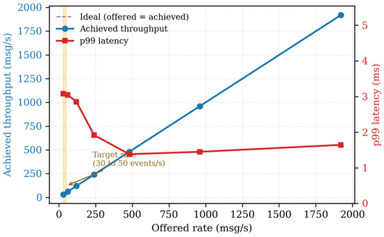
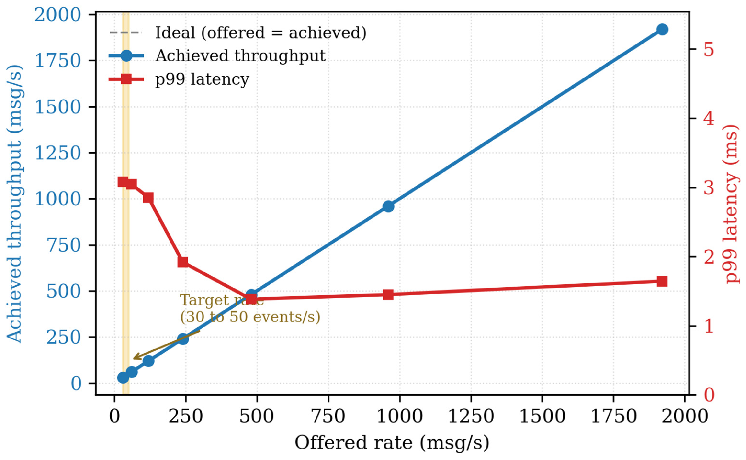
The offered rate was increased progressively from 30 to 1920 messages per second to locate the point at which the broker ceases to sustain the demand. No such point was found within the range examined: the achieved throughput follows the offered rate throughout, packet loss remains zero, and the median latency in fact decreases from 2.07 ms at 30 Hz to 1.02 ms at 1920 Hz, a consequence of more frequent writes keeping the transmission path active. Figure 9 presents the result. A sustained campaign of 28,800 messages at 960 messages per second, corresponding to 30 continuous seconds, confirmed the behavior for the three quality-of-service levels without loss, at a broker processor occupancy of 8.2 percent on average and 14.4 percent at the peak. The messaging layer therefore sustains at least 38 times the upper bound of the target rate of 30 to 50 defect events per second implied by industrial line-scan acquisition, on a single-board computer of modest specification.

Figure 9. Achieved throughput and 99th-percentile latency as a function of the offered rate. The achieved throughput follows the offered rate over the whole range examined, without packet loss, and no saturation point was reached. The shaded band indicates the target rate implied by industrial line-scan acquisition.

5.5.4. Broker Failure and Recovery

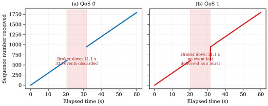
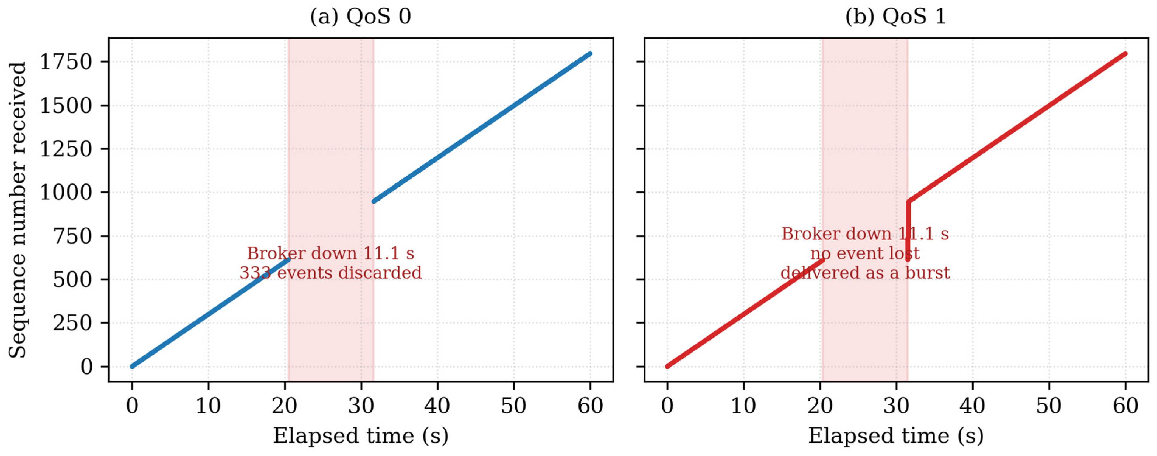
To characterize the behavior of the layer under transient infrastructure disruption, the broker was deliberately terminated during an ongoing campaign and restarted after approximately ten seconds, with the consequences quantified through sequence-number tracking. The experiment was repeated three times for QoS 0 and three times for QoS 1. Figure 10 shows one repetition of each.

Figure 10. Sequence number received against elapsed time during a deliberate broker outage of approximately eleven seconds. (a) Under QoS 0, the events issued during the outage are discarded. (b) Under QoS 1, no event is lost, but the queued events are delivered as a burst upon reconnection, with tail latencies of the order of seconds.

The two levels fail in qualitatively different ways. Under QoS 0, the events issued during the outage are discarded, with a consistent loss of 18.5 percent of the campaign across the three repetitions and no increase in the latency of the events that were delivered. Under QoS 1, the client library retains the events and delivers them as a burst upon reconnection: two of the three repetitions showed no loss at all, with 305 and 304 events delivered late and tail latencies reaching 11.1 s, while the third showed partial retention, with 14.4 percent of the events lost and only 43 delivered late. The variability of this third repetition is itself informative, since it indicates that queueing behavior depends on the client-side buffering conditions at the moment of reconnection and is therefore not a property on which a deployment can rely.

The consequence for the proposed architecture is a design conclusion of direct operational relevance. The delivery guarantee of MQTT is semantic rather than temporal: a message is eventually delivered, but not within a bounded time window. For a real-time inspection system, in which an alert that reaches the operator after the material has left the inspection window is operationally useless, neither failure mode is acceptable as it stands. An event discarded and an event delivered eleven seconds late are equivalent from the standpoint of the production line. The architecture must therefore combine QoS 1 with an application-level policy of temporal validity, for which the message expiry interval introduced in MQTT version 5.0 provides a standard mechanism, together with an explicit acquisition timestamp in the payload so that a late event can be recognized as such by the consumer and routed to the historical record rather than to the alerting path. This recommendation is reflected in Table 10.

5.5.5. Scope of the Validation

The validation reported in this subsection concerns the messaging layer of the architecture, which is the component that mediates between the edge inference node and the cloud analytics layer. The inference node itself has not been executed on embedded hardware, as stated in Section 5.4, and the cloud analytics layer is presented as a design specification rather than as an implemented system. The bench reproduces the payload structure, the event rate, and the concurrent process-variable streams of the target deployment, but not the electromagnetic environment, the network topology, or the operational duty cycle of a rolling mill, and the results should be read accordingly.

6. Open Challenges and Future Directions

Several limitations of the present experimental work should be acknowledged. First, the experiments were conducted entirely on a conventional workstation GPU; no results are reported for embedded edge hardware such as the Jetson Nano or Raspberry Pi. The performance of the trained model on such devices, in terms of both latency and power consumption, requires dedicated evaluation.

Second, the input resolution was reduced from the original 256 × 1600 pixels to 128 × 800 pixels due to GPU memory constraints. This reduction may affect detection sensitivity for very small or fine-grained defects. Future work should evaluate the model at full or intermediate resolutions with higher-capacity hardware.

Third, the dataset used does not include process metadata such as temperature, rolling force, or speed, and the Severstal imagery provides no synchronized thermomechanical measurements. Integrating such variables through multimodal learning is a promising direction for improving defect-to-process correlations. A complementary direction is offered by thermodynamically consistent, energy-based formulations, of which the Deep Energy Method [26] and its neural-operator extension VINO [27] are representative: both solve forward problems by minimizing an energy functional over a domain with a known governing equation, boundary conditions, and material parameters. Their application to surface inspection is not immediate, for the two reasons that we state explicitly. Segmentation from photographs is an inverse vision task for which no governing equation maps image intensity to a defect mask, and the publicly available imagery carries none of the thermal, force, or strain fields that such a formulation requires as input. Both directions therefore depend on a purpose-collected dataset pairing imagery with synchronized process telemetry, and are left as future work rather than applied superficially to a vision-only benchmark.

Fourth, while the full IIoT pipeline has not yet been physically deployed, the experimental results presented here constitute a proof of concept for the core computational component of the proposed architecture. The U-Net model that would operate as the edge inference node was trained, validated on 1886 unseen images, and benchmarked at approximately 22.7 ms per image under real execution conditions. This provides a reference measurement of the computational cost of the central processing stage and an empirical starting point upon which the remaining architectural layers, namely the MQTT communication pipeline, the cloud analytics layer, and the hardware integration, can be progressively built and validated in future work. The discussions in Section 4.4 and Section 5, and Section 5.4 are intended precisely to inform and structure that implementation path, grounding the architectural decisions in measured inference performance rather than theoretical assumptions.

Taken together, the limitations identified above delineate five structurally significant open challenges for practitioners and researchers seeking to implement IIoT-integrated deep learning inspection in real steel production environments, which are summarized in Table 10.

Table 10. Open challenges for IIoT-integrated deep learning inspection in steel manufacturing, with corresponding research directions.

Challenge	Description	Research Direction
Domain gap and distribution shift	Benchmark datasets such as Severstal do not fully represent live production conditions. Illumination drift, optical contamination, scale deposits, and process-state variability cause model performance to degrade after deployment, often without observable warning.	Self-supervised learning, frequency-decoupling, and unsupervised domain adaptation (UDA) frameworks tailored for real-time steel strip surface inspection under changing industrial operational environments [28].
Absence of process metadata integration	Current models detect defects in isolation from causal process variables (temperature, rolling force, speed). This limits their utility for root-cause analysis and closed-loop process control, which are the highest-value applications of IIoT in steelmaking.	Multimodal deep learning architectures fusing high-speed visual defect streams with time-series SCADA/IIoT sensor data to establish predictive correlation models between defect patterns and steel processing parameter windows [29].
Hardware–software co-optimization for embedded inference	Achieving sub-20 ms latency on constrained edge devices requires quantization, pruning, and hardware-specific compilation steps (e.g., TensorRT, ONNX Runtime) that are not yet standardized. Model accuracy can degrade significantly under aggressive INT8 quantization for fine-grained defect segmentation.	Structured pruning, knowledge distillation, and INT8 hardware-aware compilation specifically optimized for edge-AI vision architectures deployed in high-speed steel rolling lines [30].
IIoT connectivity in legacy industrial environments	Steel plants typically operate legacy fieldbus infrastructure (PROFINET, EtherCAT, Modbus) alongside modern IP-based networks. Protocol heterogeneity, cybersecurity requirements under IEC 62443, and network reliability constraints are orthogonal to model performance but equally determinant of system viability.	Deploying unified OPC UA architectures alongside lightweight MQTT-over-TLS edge gateways enables seamless protocol translation and secure OT/IT convergence, leveraging deterministic networking to integrate legacy brownfield steel assets without disrupting real-time PLC control [31].
Lack of standardized end-to-end evaluation benchmarks	Published works report model accuracy in isolation, without standardized metrics for end-to-end system performance encompassing inference latency, pipeline availability, integration overhead, and defect-to-alert delay. This makes comparative assessment across solutions difficult and limits reproducible progress.	Community-driven evaluation frameworks incorporating real-time system throughput, energy consumption, and hardware specifications alongside detection accuracy in industrial steel mills [32].

Table 10. Open challenges for IIoT-integrated deep learning inspection in steel manufacturing, with corresponding research directions.

Challenge	Description	Research Direction
Domain gap and distribution shift	Benchmark datasets such as Severstal do not fully represent live production conditions. Illumination drift, optical contamination, scale deposits, and process-state variability cause model performance to degrade after deployment, often without observable warning.	Self-supervised learning, frequency-decoupling, and unsupervised domain adaptation (UDA) frameworks tailored for real-time steel strip surface inspection under changing industrial operational environments [28].
Absence of process metadata integration	Current models detect defects in isolation from causal process variables (temperature, rolling force, speed). This limits their utility for root-cause analysis and closed-loop process control, which are the highest-value applications of IIoT in steelmaking.	Multimodal deep learning architectures fusing high-speed visual defect streams with time-series SCADA/IIoT sensor data to establish predictive correlation models between defect patterns and steel processing parameter windows [29].
Hardware–software co-optimization for embedded inference	Achieving sub-20 ms latency on constrained edge devices requires quantization, pruning, and hardware-specific compilation steps (e.g., TensorRT, ONNX Runtime) that are not yet standardized. Model accuracy can degrade significantly under aggressive INT8 quantization for fine-grained defect segmentation.	Structured pruning, knowledge distillation, and INT8 hardware-aware compilation specifically optimized for edge-AI vision architectures deployed in high-speed steel rolling lines [30].
IIoT connectivity in legacy industrial environments	Steel plants typically operate legacy fieldbus infrastructure (PROFINET, EtherCAT, Modbus) alongside modern IP-based networks. Protocol heterogeneity, cybersecurity requirements under IEC 62443, and network reliability constraints are orthogonal to model performance but equally determinant of system viability.	Deploying unified OPC UA architectures alongside lightweight MQTT-over-TLS edge gateways enables seamless protocol translation and secure OT/IT convergence, leveraging deterministic networking to integrate legacy brownfield steel assets without disrupting real-time PLC control [31].
Lack of standardized end-to-end evaluation benchmarks	Published works report model accuracy in isolation, without standardized metrics for end-to-end system performance encompassing inference latency, pipeline availability, integration overhead, and defect-to-alert delay. This makes comparative assessment across solutions difficult and limits reproducible progress.	Community-driven evaluation frameworks incorporating real-time system throughput, energy consumption, and hardware specifications alongside detection accuracy in industrial steel mills [32].

7. Conclusions

This paper addressed the problem of automated surface defect detection in hot-rolled steel from an Industrial Internet of Things perspective, combining experimental deep learning validation with a structured architectural proposal for edge–cloud integration. Two complementary contributions were presented.

The first contribution is experimental and methodological. Re-evaluating U-Net segmentation of Severstal steel defects under a leakage-free, defect-stratified split yields three lessons. First, pixel accuracy is misleading under extreme class imbalance: a trivial all-background predictor (96.66%) outscores the trained U-Net (95.77%), so Dice, IoU, precision, and recall with confidence intervals must be the reporting standard. Second, a compact from-scratch U-Net (0.49 M parameters, 38.6 ms/image) reaches a Dice of 0.42, whereas an ImageNet-pretrained DeepLabV3+ model reaches 0.68 at 37 times the parameters, an explicit accuracy-versus-footprint trade-off for edge deployment. Third, performance is dominated by defect areas (fine defects are hardest) and is most vulnerable to occlusion and sensor noise, which defines concrete robustness priorities for field deployment.

Two further lessons emerge from the messaging layer, whose characterization over 158,500 messages is reported in Section 5.5. The first concerns host and transport configuration. A factorial experiment over the four combinations of the Nagle algorithm at the two ends of the publish–subscribe chain shows that the socket configuration of the broker, and not that of the publisher, determines end-to-end latency. Disabling the algorithm at the publisher alone changes the median latency from 33.09 ms to 31.03 ms, whereas disabling it at the broker reduces it to 1.88 ms, a factor of seventeen, irrespective of the client setting. A second effect of the same nature, the power management of the network interface on the publishing host, produced a first-message latency of up to 50 ms that was the slowest sample of an entire run, and disappeared once the feature was disabled. Once host and transport are correctly configured, the level with delivery acknowledgment becomes indistinguishable in latency from the level without it, which makes the guarantee available at no measurable cost. The second lesson concerns failure: the delivery guarantee of MQTT is semantic rather than temporal, so that a broker outage causes events either to be discarded or to be delivered as a burst several seconds later, and an alert that arrives after the material has left the inspection window is as useless as one that never arrives. Both observations point in the same direction: the practical bottleneck for real-time defect notification is not the inference latency of the model but the configuration and the temporal semantics of the integration layer.

The second contribution is architectural. Grounded in the inference performance obtained, a three-layer IIoT architecture was proposed in which the trained U-Net model operates as the edge inference node, processing images locally and publishing structured defect events via MQTT to a cloud analytics layer responsible for historical storage, quality dashboards, and periodic model retraining. The architecture follows established IIoT layering principles documented in the steel casting monitoring and edge–cloud defect detection literature, and is explicitly designed as an implementable framework rather than a theoretical construct. A comparative assessment of five edge hardware platforms across seven deployment dimensions (Table 7) was provided to support practitioners in hardware selection, and five structurally significant open challenges for IIoT-integrated inspection systems were identified and mapped to concrete research directions (Table 10).

Together, these contributions position deep learning-based steel surface inspection within the broader context of Industry 4.0 and IIoT-enabled manufacturing. The results delimit an accuracy-versus-footprint design space for the edge inference node rather than prescribing a single model, and show that the integration layers, which are usually assumed rather than measured, are the ones that determine operational readiness. Future work will focus on three directions: physical deployment and latency benchmarking of the trained model on embedded edge GPU hardware; integration of process sensor streams (temperature, rolling force, speed) to enable defect-to-process correlations within the IIoT pipeline; and end-to-end validation of the proposed three-layer architecture in a laboratory or pilot production environment, with quantitative reporting of system-level metrics including pipeline availability, defect-to-alert delay, and model drift over time.

References

- Instituto Aço Brasil. Anuário Estatístico da Indústria do Aço no Brasil 2023; IABr: São Paulo, Brazil, 2024; Available online: https://www.acobrasil.org.br/site/wp-content/uploads/2023/11/Estatistica-da-Siderurgia_3o_TRI_2023.pdf (accessed on 30 June 2026).
- Konovalenko, I.; Maruschak, P.; Brevus, V. Steel surface defect detection using an ensemble of deep residual neural networks. J. Comput. Inf. Sci. Eng. 2022, 22, 014501. [Google Scholar] [CrossRef] [Scilit]
- Neogi, N.; Mohanta, D.K.; Dutta, P.K. Review of vision-based steel surface inspection systems. EURASIP J. Image Video Process. 2014, 2014, 50. [Google Scholar] [CrossRef] [Scilit]
- Papaefthymiou, S.; Tzevelekou, T.; Antonopoulos, A.; Gypakis, A. Typical defects in plate and long steel products. Int. J. Struct. Integr. 2016, 7, 645–655. [Google Scholar] [CrossRef] [Scilit]
- Sun, X.; Gu, J.; Tang, S.; Li, J. Research progress of visual inspection technology of steel products: A review. Appl. Sci. 2018, 8, 2195. [Google Scholar] [CrossRef] [Scilit]
- Zhang, F.; Liu, M.; Zhou, Z.; Shen, W. An IoT based online monitoring system for continuous steel casting. IEEE Internet Things J. 2016, 3, 1355–1363. [Google Scholar] [CrossRef] [Scilit]
- Ronneberger, O.; Fischer, P.; Brox, T. U-Net: Convolutional networks for biomedical image segmentation. In Proceedings of the 18th International Conference on Medical Image Computing and Computer-Assisted Intervention (MICCAI 2015), Munich, Germany, 5–9 October 2015; Springer: Cham, Switzerland, 2015; pp. 234–241. [Google Scholar] [CrossRef] [Scilit]
- Luo, Q.; Fang, X.; Liu, L.; Yang, C.; Sun, Y. Automated visual defect detection for flat steel surface: A survey. IEEE Trans. Instrum. Meas. 2020, 69, 626–644. [Google Scholar] [CrossRef] [Scilit]
- ASTM A240/A240M-23; Standard Specification for Chromium and Chromium-Nickel Stainless Steel Plate, Sheet, and Strip for Pressure Vessels and for General Applications. ASTM International: West Conshohocken, PA, USA, 2023.
- Lin, D.; Li, Y.; Prasad, S.; Nwe, T.L.; Dong, S.; Oo, Z.M. CAM-guided multi-path decoding U-Net with triplet feature regularization for defect detection and segmentation. Knowl.-Based Syst. 2021, 228, 107272. [Google Scholar] [CrossRef] [Scilit]
- Konovalenko, I.; Maruschak, P.; Brezinová, J.; Prentkovskis, O.; Brezina, J. Research of U-Net-based CNN architectures for metal surface defect detection. Machines 2022, 10, 327. [Google Scholar] [CrossRef] [Scilit]
- Neven, R.; Goedemé, T. A multi-branch U-Net for steel surface defect type and severity segmentation. Metals 2021, 11, 870. [Google Scholar] [CrossRef] [Scilit]
- Song, G.; Song, K.; Yan, Y. EDRNet: Encoder–Decoder Residual Network for Salient Object Detection of Strip Steel Surface Defects. IEEE Trans. Instrum. Meas. 2020, 69, 9709–9719. [Google Scholar] [CrossRef] [Scilit]
- Liu, B.; Yang, B.; Zhao, Y.; Li, J. Low-pass U-Net: A segmentation method to improve strip steel defect detection. Meas. Sci. Technol. 2023, 34, 035405. [Google Scholar] [CrossRef] [Scilit]
- Ashrafi, S.; Teymouri, S.; Etaati, S.; Khoramdel, J.; Borhani, Y.; Najafi, E. Steel surface defect detection and segmentation using deep neural networks. Results Eng. 2025, 25, 103972. [Google Scholar] [CrossRef] [Scilit]
- Sun, H.; Xia, L.; Zhou, Y.; Qian, W.; Wang, W.; Zhang, K. Online detection and evaluation of weld surface defects based on lightweight network VGG16-UNet and laser scanning. J. Manuf. Process. 2024, 129, 292–306. [Google Scholar] [CrossRef] [Scilit]
- Ibrahim, A.A.M.; Tapamo, J.R. Transfer learning-based approach using new convolutional neural network classifier for steel surface defects classification. Sci. Afr. 2024, 23, e02066. [Google Scholar] [CrossRef] [Scilit]
- Kaggle. Severstal: Steel Defect Detection. Available online: https://www.kaggle.com/c/severstal-steel-defect-detection (accessed on 30 June 2026).
- Kaggle. Severstal RLE Annotation Format. Available online: https://www.kaggle.com/c/severstal-steel-defect-detection/overview/evaluation (accessed on 30 June 2026).
- NVIDIA Corporation. Jetson Orin NX Series Data Sheet; NVIDIA: Santa Clara, CA, USA, 2023; Available online: https://developer.nvidia.com/embedded/jetson-modules (accessed on 30 June 2026).
- OASIS Standard. MQTT Version 5.0. Available online: https://docs.oasis-open.org/mqtt (accessed on 30 June 2026).
- Seliem, M.; Roedig, U.; Sreenan, C.; Pesch, D. BiLSTM-based fault anticipation for predictive activation of FRER in time-sensitive industrial networks. IoT 2025, 6, 60. [Google Scholar] [CrossRef] [Scilit]
- Sisinni, E.; Saifullah, A.; Han, S.; Jennehag, U.; Gidlund, M. Industrial Internet of Things: Challenges, opportunities, and directions. IEEE Trans. Ind. Inform. 2018, 14, 4724–4734. [Google Scholar] [CrossRef] [Scilit]
- Merenda, M.; Porcaro, C.; Iero, D. Edge machine learning for AI-enabled IoT devices: A review. Sensors 2020, 20, 2533. [Google Scholar] [CrossRef] [Scilit] [PubMed]
- Shi, W.; Cao, J.; Zhang, Q.; Li, Y.; Xu, L. Edge computing: Vision and challenges. IEEE Internet Things J. 2016, 3, 637–646. [Google Scholar] [CrossRef] [Scilit]
- Samaniego, E.; Anitescu, C.; Goswami, S.; Nguyen-Thanh, V.M.; Guo, H.; Hamdia, K.; Zhuang, X.; Rabczuk, T. An energy approach to the solution of partial differential equations in computational mechanics via machine learning: Concepts, implementation and applications. Comput. Methods Appl. Mech. Eng. 2020, 362, 112790. [Google Scholar] [CrossRef] [Scilit]
- Eshaghi, M.S.; Anitescu, C.; Thombre, M.; Wang, Y.; Zhuang, X.; Rabczuk, T. Variational physics-informed neural operator (VINO) for solving partial differential equations. Comput. Methods Appl. Mech. Eng. 2025, 437, 117785. [Google Scholar] [CrossRef] [Scilit]
- Zhou, X.; Zhang, Y.; Wang, L. Feature Decoupling-Guided Annotation Framework for Surface Defects on Steel Strips. Electronics 2025, 14, 2304. [Google Scholar] [CrossRef] [Scilit]
- Alonso, M.A.; Castro, J.L.A.; Perez, R.E.A. Multi-Sensor Data Fusion for Real-Time Surface Quality Control in Automated Machining Systems. Sensors 2018, 18, 4381. [Google Scholar] [CrossRef] [Scilit] [PubMed]
- Lv, Y.; Yang, J.; Liu, H. A lightweight convolutional neural network for surface defect detection in strip steel. J. Real-Time Image Process. 2024, 21, 45. [Google Scholar]
- Silva, A.M.L.; Basso, M.; Santos, R. Integration of Legacy Industrial Equipment in a Building-Management System Industry 5.0 Scenario. Sensors 2024, 24, 5210. [Google Scholar] [PubMed]
- Toth, K.; Singhal, M.; Chauhan, D.; Polra, J.; Zhou, C.; Page, G.; Fisher, C. A Dual-Model Approach to Industrial Safety: Computer Vision for PPE Compliance and Hazard-Zone Monitoring in Steel Production. Integr. Mater. Manuf. Innov. 2026, 15, 326–340. [Google Scholar] [CrossRef] [Scilit]
Disclaimer/Publisher’s Note: The statements, opinions and data contained in all publications are solely those of the individual author(s) and contributor(s) and not of MDPI and/or the editor(s). MDPI and/or the editor(s) disclaim responsibility for any injury to people or property resulting from any ideas, methods, instructions or products referred to in the content. |
© 2026 by the authors. Licensee MDPI, Basel, Switzerland. This article is an open access article distributed under the terms and conditions of the Creative Commons Attribution (CC BY) license.