


Abstract
The continued growth of the Android ecosystem has been accompanied by an escalating volume of malicious applications, motivating the development of detection methods that are simultaneously accurate, transparent, and resilient to evasion. Graph-based learning has emerged as a powerful paradigm for Android malware detection because it represents applications as function call graphs (FCGs) that preserve both semantic node attributes and structural relationships. However, most existing graph neural network (GNN) detectors rely on a single learning architecture, offer little insight into their decisions, and are rarely evaluated against adversarial manipulation. This paper presents XGCN-GAT, a hybrid framework that processes each application graph in parallel through Graph Convolutional Network (GCN) and Graph Attention Network (GAT) branches and fuses their embeddings for classification. Beyond detection, the framework is subjected to a three-part trustworthiness evaluation: (i) post hoc explainability using SHapley Additive exPlanations (SHAP) and GNNExplainer, (ii) a quantitative assessment of explanation faithfulness, stability, and cross-explainer agreement, and (iii) a feature-space adversarial robustness analysis under an add-only threat model. On a Drebin-based dataset of 10,249 applications, the final XGCN-GAT model attains 95.65% accuracy and 97.8% AUC on a held-out test set of 2000 applications. In a controlled comparison with its individual branches under the same training protocol, the hybrid is significantly more accurate than the GCN branch at two of three model widths and on par with the GAT branch in accuracy at every width, while missing the fewest malicious applications at every width. The explainability analysis identifies permission features as the largest contributor in aggregate, while method-type features show the largest per-feature attribution and the strongest impact under category-level ablation. The robustness analysis reveals a meaningful feature-space vulnerability under the defined add-only threat model: greedy perturbations achieve successful evasion with a small number of added features but plateau before complete evasion, whereas explanation-guided perturbations achieve higher ultimate evasion and require no model queries during the attack once feature attributions are available (in our experiments, these attributions were computed with full model access), outperforming random and FGSM attacks. Naive adversarial retraining yields no measurable improvement. These results establish XGCN-GAT as an effective detector while providing a candid, reproducible account of the interpretability and security limitations that remain open for graph-based malware detection.
1. Introduction
Over the past decade, the rapid expansion of mobile applications has been accompanied by a substantial increase in malicious software targeting mobile devices [1]. Android, as the dominant mobile operating system worldwide, has become a primary target for attackers owing to its open-source architecture and widespread adoption [2]. While openness has enabled rapid application development and distribution, it has also facilitated the propagation of applications that conceal malicious behaviour. Consequently, developing detection techniques that are accurate, transparent, and resilient has become a pressing challenge for the security community.
Traditional detection methods, such as signature-based approaches, are effective against known threats but struggle with new, obfuscated, or evolving variants [3]. To overcome these limitations, research has increasingly turned to machine learning and deep learning techniques capable of learning discriminative patterns directly from data [4]. Such techniques may be applied through static analysis, which inspects application code without execution, or dynamic analysis, which observes runtime behaviour [5]. Because of its efficiency, scalability, and low computational overhead, static analysis remains one of the most widely adopted approaches for large-scale Android malware detection.
Recent studies have shown that representing Android applications as graphs provides a more informative description of application behaviour than flat feature vectors [6]. These methods model applications as function call graphs (FCGs), where nodes represent methods or APIs and edges capture caller–callee relationships [7]. Among graph neural network (GNN) architectures, Graph Convolutional Networks (GCNs) [8] learn global structural patterns through neighbourhood aggregation and have achieved strong detection performance [9,10,11]. Graph Attention Networks (GATs) [12], in turn, assign adaptive importance to different nodes and calls, allowing the model to focus on the most informative graph regions [13,14]. Despite the individual success of these architectures, most existing detectors employ either GCN or GAT in isolation, limiting their ability to jointly capture global structure and locally salient interactions.
Two further concerns have received comparatively little attention in graph-based Android malware detection. The first is transparency: most GNN detectors behave as black boxes, offering limited insight into the features and structures that drive their predictions [15,16]. Explainability techniques such as SHAP [17] and GNNExplainer [18] have begun to address this gap by identifying influential features, nodes, and subgraphs [19,20,21,22], yet their reliability is seldom quantified for graph-based detectors. The second concern is robustness: malware authors actively adapt their applications to evade detection, but the resilience of hybrid graph detectors to adversarial feature manipulation is rarely measured. A detector that is accurate on a static benchmark may nevertheless be trivially evaded in practice.
To address these gaps, this paper proposes XGCN-GAT, an explainable and robustness-aware hybrid framework for Android malware detection. The framework models each application as an FCG and processes it in parallel through GCN and GAT branches, fusing their embeddings to classify applications as benign or malicious. Crucially, detection accuracy is only the starting point of the evaluation. We additionally (i) generate feature-level and graph-level explanations using SHAP and GNNExplainer, (ii) quantify the faithfulness, stability, and mutual agreement of those explanations, and (iii) evaluate the model against feature-space adversarial evasion under an add-only threat model restricted to manifest-level declarations, whose practical feasibility we analyse explicitly.
This study is organised around four research questions:
- RQ1
- (Detection) Does the parallel fusion of GCN and GAT branches improve detection over each branch trained in isolation under an identical protocol, and does the result carry over to an independently collected dataset? (Section 4.2).
- RQ2
- (Explanation content) Which feature categories drive the model’s decisions, and do attribution-based (SHAP) and removal-based (ablation) notions of importance agree? (Section 4.3 and Section 4.3.2).
- RQ3
- (Explanation quality) How faithful, stable and mutually consistent are the explanations produced by SHAP and GNNExplainer? (Section 4.3.1).
- RQ4
- (Robustness) How vulnerable is the detector to add-only, feature-space evasion, do explanations help an attacker, and does simple adversarial retraining mitigate the vulnerability? (Section 4.4).
The main contributions of this work are summarised as follows:
- We propose XGCN-GAT, a hybrid GNN framework that combines graph convolution and graph attention within a parallel architecture to learn complementary structural representations from Android application graphs, and we compare it with its GCN and GAT branches trained in isolation under an identical protocol, with confidence intervals and paired significance tests, complemented by a sensitivity analysis of its hyper-parameters (RQ1).
- We integrate two complementary post hoc explainers, SHAP and GNNExplainer, and, extending earlier evaluations of explanation methods for Android malware detectors operating on flat feature vectors [23,24] to a hybrid GNN detector, we quantitatively evaluate the resulting explanations in terms of faithfulness, stability, and cross-explainer agreement, rather than presenting them as self-evidently correct (RQ2, RQ3).
- We conduct a feature-space adversarial robustness analysis under an add-only threat model, comparing random, greedy, gradient-based, and explanation-guided attacks, and we probe a lightweight adversarial-retraining defence; we also analyse how each feature manipulation would be realised in an APK, and we distinguish the resulting feature-space vulnerability from real-world evasion (RQ4).
- We distinguish aggregate, per-feature and ablation-based notions of feature importance, showing that permission features dominate aggregate attribution whereas method-type features carry the largest per-feature attribution and the largest ablation effect, and we provide a candid discussion of the interpretability and security limitations that remain open.
The remainder of this paper is organised as follows. Section 2 reviews related work on graph-based Android malware detection and explainable GNNs. Section 3 describes the proposed XGCN-GAT framework. Section 4 presents the experimental setup and results, covering detection performance, explainability, explanation quality, and robustness. Section 5 discusses the findings, Section 6 outlines future work, and Section 7 concludes.
2. Related Work
2.1. Graph-Based Android Malware Detection
Graph representations have become a cornerstone of modern Android malware detection because they preserve the interactions between application components that flat feature vectors discard [6,16]. Applications are commonly modelled as function call graphs, control flow graphs, or API-dependency graphs, and a GNN is then trained to classify the resulting structures. GCN-based detectors learn global structural regularities through neighbourhood aggregation and have reported strong benchmark performance [9,11,25]. To improve resilience against obfuscation, Lu et al. [10] combined subgraph extraction with a denoising GCN, mitigating the influence of noisy or injected code. Attention-based approaches instead weight neighbours adaptively: heterogeneous and knowledge-graph attention networks have been proposed to capture richer relationships among application entities [13,14]. Other detectors combine several views of an application: Yumlembam et al. [26] fuse GraphSAGE embeddings of API graphs with permission and intent features, and DeepCatra [27] combines abstract flow graphs with a recurrent model over call traces to critical APIs. These studies consistently show that structural information improves detection, but they typically commit to a single architectural family, leaving the complementary strengths of convolution and attention only partially exploited.
2.2. Explainability in Graph-Based Detection
As GNN detectors are considered for deployment, the opacity of their decisions has become a recognised obstacle [15,16]. Post hoc explainers aim to expose the factors behind a prediction. SHAP attributes a prediction to individual input features through Shapley values grounded in cooperative game theory [17,28], while GNNExplainer identifies a compact subgraph and feature subset that maximise mutual information with the prediction [18,29]. Surveys and benchmarks of GNN explainers organise these methods into families and show that no explainer dominates across metrics and datasets [30,31]. Recent security-oriented work has begun to apply these tools: interpretable intrusion-detection models integrate SHAP to expose feature-level reasoning [21], and graph-reduction pipelines use GNNExplainer to surface influential subgraphs in malware graphs [22]. A graph-based interpretable framework for Android detection was also proposed by Fan et al. [15]. However, these works largely treat explanations as trustworthy by construction. Quantitative evaluation of explanations has previously been carried out for security applications, including Android malware detection, by Warnecke et al. [23], who compared explanation methods in terms of descriptive accuracy, sparsity, stability and robustness, and by Fan et al. [24], who proposed sanity checks for explanations of Android malware classifiers. These studies considered detectors operating on flat feature vectors; our work extends this line of evaluation to a hybrid graph neural network and to the combination of a feature-level (SHAP) and a structure-level (GNNExplainer) explainer. The reliability of the explanations themselves—whether they are faithful to the model, stable under small input changes, and consistent across methods—remains underexplored for graph-based malware detectors and is a central concern of the present paper.
2.3. Adversarial Evasion of Learning-Based Detectors
Learning-based malware detectors are attractive targets for evasion. In the Android domain, the practical attacker is constrained: capabilities such as permissions, hardware requests, and intent filters can generally be added to an application without breaking its functionality, whereas removing them risks disabling the malicious payload. This asymmetry gives rise to the widely used add-only, feature-space threat model, which was used in early adversarial studies of Drebin-based detectors [32,33]. Problem-space attacks, which must produce valid and functional APKs, face further constraints [34], and structural attacks against graph-based detectors modify the function call graph itself [35,36]. Explanations have also been shown to guide attacks on malware classifiers [37]. Although adversarial robustness is well studied for image and Windows Portable Executable file (PE-file) classifiers, its interaction with hybrid graph detectors and with explanation methods has received limited attention. We therefore evaluate XGCN-GAT against a spectrum of add-only attacks and, in particular, examine whether the explanations that make the model transparent also make it easier to attack.
3. The Proposed XGCN-GAT Framework
The proposed framework comprises three stages as illustrated in Figure 1: graph construction and feature extraction, hybrid graph-based classification, and a trustworthiness layer that combines post hoc explainability with adversarial robustness analysis. Each stage is described below.
Figure 1.
High-level pipeline of the proposed XGCN-GAT framework: (i) static construction of the function call graph with a manifest-level root node and 209-dimensional node features; (ii) classification by the hybrid GCN–GAT network (detailed in Figure 2); and (iii) the trustworthiness analysis, comprising post hoc explanations (SHAP, GNNExplainer), their quantitative evaluation and category ablation, and add-only adversarial attacks with adversarial retraining.
3.1. Graph Construction and Feature Extraction
Each Android application package (APK) is analysed statically to produce a function call graph in which nodes correspond to methods and edges represent caller–callee relationships. The adjacency matrix is symmetrised, so each call relation is stored as an undirected edge, and information flows in both directions during message passing. Static analysis is performed using Androguard [38], which parses the DEX bytecode and constructs a cross-reference analysis over the methods it resolves. Each graph node is identified by the Smali-form combination of the class name and method name (e.g., Lcom/example/Foo;->bar). Method parameters and return types are not included in the identifier; consequently, overloaded methods belonging to the same class are represented by a single node. For each resolved method, the outgoing invocations reported by the cross-reference analysis are examined, and an edge is added only when the target method is also registered in the analysis. Calls whose target methods cannot be statically resolved, including dynamically resolved or externally unavailable targets, are omitted from the graph rather than represented by placeholder nodes. Thus, the resulting graph contains only statically resolvable method-call relationships. This is a known limitation of static call-graph analysis [39]. Framework and third-party library methods that are successfully resolved are retained as regular graph nodes and subsequently assigned the corresponding API-method category described below, so the graph records which framework APIs are reachable from application code while retaining method-level granularity, as in node-labelled function call graph detectors [40]. Edges are binary, such that repeated invocations between the same source and target methods are represented by a single edge; invocation frequency is therefore not modelled. At a broader level, static analysis enables method-call dependencies to be characterised without executing the application, making it suitable for large-scale analysis.
Each graph additionally contains a synthetic root node at index 0, denoted dummyMain, which is connected to all other nodes. This node provides a common entry point for the graph and serves as a global representation for application-level information declared in the Android manifest, which cannot be attached to any particular node. Since it does not correspond to a real method, it receives neither an API-method category nor the suspicious-API flag; it carries only the manifest-level features described below.
To characterise each node, a 209-dimensional feature vector is assigned using statically extracted Android characteristics grouped into five complementary categories: (1) API method categories, distinguishing System, Third-Party, Component, and Other APIs (four dimensions). The category is determined from the method’s class path by the following rules, evaluated in order, with the first match deciding the label. A method is labelled Component API when its class path corresponds to an Android application component, such as an Activity, Service, Receiver, or Provider. Otherwise, it is labelled System API when its class path begins with Landroid or Ljava, or when its second path segment is android or java. If neither condition applies, the method is labelled Third-Party API when its second package segment is google, facebook, or yahooapis; all remaining methods are assigned to Other. The synthetic entry node, dummyMain, does not receive a method-type label; (2) permission features, covering 91 commonly requested Android permissions; (3) suspicious API features, capturing security-critical calls such as device-identifier retrieval, SMS dispatch, and telephony access. This category is encoded as a single binary indicator that is set when a method matches one of fourteen predefined security-relevant APIs such as TelephonyManager.getDeviceId and TelephonyManager.getImei; (4) hardware features, describing requested capabilities such as telephony, Wi-Fi, Bluetooth, GPS, and camera (60 dimensions); and (5) intent-filter features, characterising entry points and inter-component communication (53 dimensions: 36 intent actions and 17 intent categories). All features are binary presence indicators. The index of every dimension is fixed by a single mapping table (Table 1), which is identical for all applications, is never re-derived per sample, and is released together with the code as feature_map.json. The complete list of the 209 features, with their index, category and Android protection level (permissions), is given in Supplementary Table S1. Categories (1) and (3) are local properties assigned to the specific method nodes where they occur. In contrast, categories (2) and (4), corresponding to permissions and hardware features, represent application-level declarations extracted from the manifest. These declarations are propagated to graph nodes at three levels. (i) Application level: each permission declared in the manifest, and each <uses-feature> hardware declaration, activates the corresponding feature dimension on the root node. (ii) Method level: declared permissions are additionally propagated to individual methods associated with those permissions through a permission-to-API mapping compiled from the published PScout mappings [41] (Froyo through API 22, including the content-provider field-permission tables) and converted to Smali signatures. When a mapped API method is present in the graph, the corresponding permission feature is activated on that node in addition to the root node. If no mapping is available for a permission, only its application-level representation is retained, without affecting any other feature dimensions. (iii) Component level: an android:permission attribute declared on <application>, <activity>, or <receiver> activates the corresponding permission feature on the root node and on every method whose class name matches the declaring component. Hardware features are further inferred at the node level from the permissions associated with each node according to a predefined set of Android permission-to-feature implications. For example, CAMERA activates android.hardware.camera, while ACCESS_FINE_LOCATION activates android.hardware.location and, for applications with minSdkVersion , location.gps. The same rule-based procedure is applied to the remaining predefined permission-to-hardware mappings, including Bluetooth, audio, Wi-Fi, and telephony-related features. In addition, an activity’s screenOrientation attribute activates either screen.portrait or screen.landscape on the methods belonging to that activity. The android.hardware.faketouch feature is activated on the root node when no touchscreen capability is declared. Intent-filter actions and categories are attributed to the class of the component declaring the filter and propagated to every method belonging to that class. Component names specified in relative form, beginning with a leading dot, are resolved against the application package name.
Table 1.
Exact composition of the 209-dimensional node feature vector. Indices are zero-based and identical for every application.
The five categories follow the feature families of the Drebin study [42]: hardware components (S1), requested permissions (S2) and filtered intents (S4) are represented directly; the suspicious-API flag corresponds to S7; the permission bits on permission-protected API nodes approximate used permissions (S6); and the Component method type partly reflects application components (S3). Network addresses (S8) are not used because they are high-cardinality and trivially changeable. Unlike Drebin’s open-ended feature space (more than 545,000 distinct features), a GNN requires fixed-length node attributes, and we therefore use compact vocabularies taken from the Android documentation: the normal, signature and dangerous permission lists of Android 9 (API level 28; 91 permissions), the hardware features of the <uses-feature> reference (60), and the standard intent actions (36) and categories (17). Of the 209 vocabulary entries, 154 occur in at least one application of our dataset (69 of the 91 permissions, 39 of the 60 hardware features and 41 of the 53 intent-filter entries). 99.4% of the applications declare at least one vocabulary permission, and 95.3% have at least one vocabulary intent-filter entry. Because the permission list follows a recent API level, some permissions that are frequent in older malware, such as WRITE_SMS, READ_LOGS, INSTALL_PACKAGES, GET_TASKS and WRITE_APN_SETTINGS, as well as custom permissions, are not represented. Representing manifest features as node attributes of a call graph follows earlier GCN-based detectors [43]. The contribution of each category is quantified by the ablation study in Section 4.3.2.
Following feature extraction, each application is represented by a binary sparse node-feature matrix and a binary sparse adjacency matrix A. At load time, self-loops are added to the adjacency matrix, yielding , and the node features are row-normalised as , where is the diagonal matrix of the row sums of X (all-zero rows are left unchanged). For the GCN branch, the self-loop-augmented adjacency matrix is normalised as , where is the diagonal row-sum degree matrix of . The GAT branch uses the same self-loop-augmented edge set, so both branches receive an identical graph structure. Because the call graphs are large, each graph with more than K nodes is reduced before training and inference to the subgraph induced by its K highest-degree nodes, keeping their features and the edges among them. The root node, which has the highest degree, is always retained. We use in the reduced-protocol experiments and for the final model and the branch comparison (Section 4.1); the cap affects 70.5% and 55.6% of the graphs, respectively. Combining these node attributes with FCG topology enables the model to jointly learn semantic and structural cues.
3.2. Hybrid Graph Neural Network Architecture
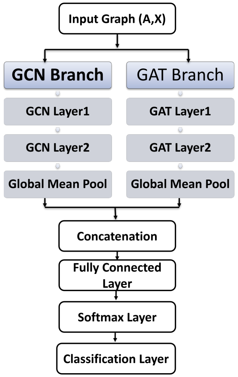
XGCN-GAT processes each graph simultaneously through two independent branches, ensuring that both branches observe the same structure and node attributes while extracting complementary characteristics. The GCN branch consists of two stacked graph convolutional layers followed by global average pooling; each layer aggregates information from neighbouring nodes to capture the overall structural organisation of the application, yielding a graph-level embedding . The GAT branch employs two graph attention layers with multi-head attention followed by the same pooling strategy; by learning adaptive attention coefficients, it emphasises the function-call relationships most relevant to classification, yielding . The GAT branch uses eight attention heads, and the hidden dimension of the GCN branch equals the concatenated GAT dimension (eight times the per-head dimension). We denote a model width by the GAT per-head dimension times the number of heads, e.g., .
The two embeddings are fused by concatenation, , so that the unified representation captures both global topology and attention-weighted local interactions. The fused vector is passed to a fully connected layer followed by a softmax activation that estimates the probability of the benign and malicious classes, and the predicted label is the class of highest probability. The network is trained end-to-end with the Adam optimiser [44], jointly optimising both branches and the classifier. The detailed XGCN-GAT architecture is illustrated in Figure 2.
Role of the root node. The root node follows the virtual-node design used in message-passing neural networks [45,46,47]. Manifest declarations describe the application as a whole; storing them on one node connected to every method avoids assigning them arbitrarily to a single method or duplicating them on all nodes, delivers application-level context to every method in one hop, and, over two layers, provides each node with a global receptive field. It also makes the add-only threat model of Section 3.4 well defined, since adding a manifest declaration changes a single node. The design has two side effects. The additional edges place all methods within two hops of one another, which can accelerate over-smoothing in deep GCNs [48], a risk limited here by using two layers. In addition, under symmetric normalisation the GCN branch scales messages to and from the root by approximately , which attenuates the manifest signal in large graphs, whereas the GAT branch can learn to up-weight root edges through its attention coefficients. This asymmetry offers a plausible explanation for the weaker performance of the GCN branch observed in the experiments (Section 4.2).
Figure 2.
Architecture of the hybrid XGCN-GAT classifier. The input graph is processed in parallel by a two-layer GCN branch and a two-layer, eight-head GAT branch; each branch is summarised by global mean pooling, and the two graph embeddings are concatenated and passed to a fully connected layer with softmax output.
3.3. Explainability Layer
To interpret the trained model, two complementary post hoc techniques are applied without altering the learned parameters. We use one explainer at the level of feature types and one at the level of graph structure. SHAP [17] is a model-agnostic, axiomatically grounded attribution method whose output (the contribution of each permission, hardware feature or method type) matches the level at which analysts reason about Android applications. GNNExplainer [18] jointly learns edge and feature masks and identifies the call-graph substructure that supports a prediction. The two methods belong to different families of GNN explanation methods [30], which allows us to assess how strongly explanations depend on the method. Other GNN explainers were not included for practical reasons: PGExplainer [49] requires training a separate explainer network, SubgraphX [50] relies on Monte Carlo tree search, which is costly on call graphs with thousands of nodes, and gradient-based attribution [51] requires a baseline input that is not well defined for binary features. Since benchmark studies show that no GNN explainer is uniformly best [31], extending the evaluation to these methods is a natural next step (Section 6).
SHAP. Shapley values are estimated with the model-agnostic KernelSHAP estimator [17], as implemented in the shap library, using 200 coalition samples per application. The players of the coalition game are the feature types (feature columns) present in the application, not individual node–feature entries; feature types absent from the application receive zero attribution. For a coalition S, the value function is the malware probability that XGCN-GAT assigns to the application’s graph after every present feature outside S has been replaced, on every node, by its background value and the features have been re-normalised; the graph topology is left unchanged. The background values are the per-feature means of the node-level feature vectors of 100 benign training applications selected at random (seed 42). Because the number of samples is small relative to the number of possible coalitions, the estimator’s default L1 regularisation retains at most ten features per application and assigns zero to the others; the global rankings therefore aggregate the ten most important features of each application. Because attributions are measured relative to this benign reference, a positive SHAP value answers the contrastive question “which features make this application look more malicious than a typical benign application?” [52]. The global-average-pooled 209-dimensional vector is used only to describe each application compactly and to aggregate attributions; it is never classified by a separate model, so the attributions explain the graph classifier itself rather than a surrogate. Attributions are analysed globally (mean absolute SHAP value per feature across the evaluation set) and at the level of correctly detected (true-positive) and missed (false-negative) malware.
This design has two consequences for interpretation. First, the attributions are made at the level of feature types: they quantify the combined effect of a feature on all nodes where it occurs but cannot indicate which nodes are responsible, which is the information provided by GNNExplainer’s edge mask. Second, because manifest-level features are stored on the single root node, their pooled values scale as with graph size, so pooled feature magnitudes should not be compared across applications of different sizes; the SHAP values themselves are unaffected, because they are measured on the model output. Finally, KernelSHAP is a sampling-based estimator whose attributions carry Monte Carlo variance [53], which is relevant to the stability results in Section 4.3.1.
GNNExplainer. We implemented GNNExplainer [18] for graph-level classification in PyTorch (version 2.7.1 with CUDA 11.8; Python 3.10.19), following the original formulation, and optimised it for 150 steps with Adam and a learning rate of 0.01 towards the class predicted by the model. The explainer learns a soft mask over all edges of the (capped) graph and a node-feature mask shared across nodes, i.e., one weight per feature type (209 values), regularised by size penalties on both masks (coefficient 0.005 each) and an entropy penalty on both masks (coefficient 0.1). The explanation subgraph consists of the edges whose mask value exceeds 0.5 together with their endpoint nodes. Although the whole graph is presented to the explainer, each node’s contribution depends only on its two-hop neighbourhood, which matches the receptive field of the two-layer branches. All explainer settings are summarised in Table 2.
Table 2.
Configuration of the explainers and of the explanation-quality evaluation.
Quantitative Evaluation of Explanation Quality
Rather than assuming the explanations are correct, we evaluate them along three axes. Faithfulness assesses whether the importance assigned by an explanation method reflects the actual influence of the identified features on the model prediction. Two complementary measures are used: comprehensiveness and sufficiency [54,55]. Comprehensiveness measures the decrease in the model’s predicted probability when the most important features identified by the explainer are removed, whereas sufficiency measures how much of the original model prediction is retained when only the identified important features are preserved. Let denote the predicted malware probability for sample x, denote the set of the top-k important features identified by the explanation method among the features present in the application, and denote the input obtained by replacing the features in with their corresponding background values on the nodes where they are present, while keeping the remaining features unchanged. The background vector is constructed by averaging the node-level feature vectors of 100 randomly selected benign training applications. denotes the input in which only the top-k features are retained, all other present features being replaced by their background values. The comprehensiveness score is defined as
where a larger value indicates that removing the important features causes a greater decrease in the predicted malware probability, suggesting a more faithful explanation. The sufficiency score is the retained probability
so that values close to indicate that the top-k features alone preserve the prediction.
Stability is measured by recomputing attributions under negligible, prediction-preserving input perturbations. Spearman’s rank correlation coefficient [56] is a non-parametric measure of the monotonic association between two ranked variables. It ranges from to 1, where values closer to 1 indicate stronger agreement between the two rankings. In this study, Spearman correlation is used to quantify the consistency of feature rankings between the original and perturbed explanations. Let denote the feature-importance (attribution) vector generated by an explainability method for the original sample x, where d is the number of input features and represents the attribution assigned to feature j. For SHAP, corresponds to the SHAP value , whereas for GNNExplainer, corresponds to the learned feature-mask value. Moreover, let denote the corresponding explanation obtained from a perturbed sample that preserves the model prediction. The Spearman stability score is computed as
where denotes Spearman’s rank correlation coefficient. Values closer to 1 indicate that the relative ordering of feature importance remains highly consistent under perturbation. In addition to ranking consistency, the overlap between the top-10 most important features in the original and perturbed explanations is quantified using the Jaccard similarity coefficient. The Jaccard similarity coefficient [57] is a set-based measure that quantifies the proportion of shared elements between two sets relative to their union. It ranges from 0 to 1, with 1 indicating identical sets. Let and denote the sets of the top-10 important features extracted from and , respectively. The Top-10 Jaccard overlap is computed as
where values closer to 1 indicate greater overlap between the two sets of top-ranked features, reflecting more stable explanations.
The cross-explainer agreement compares the global feature rankings produced by SHAP and GNNExplainer. Kendall’s [58] is a non-parametric rank correlation measure that evaluates the agreement between two rankings based on the relative ordering of pairs. Higher values indicate stronger rank agreement. In this paper, Spearman correlation and Kendall’s are used to compare the global feature rankings produced by SHAP and GNNExplainer, while Top-10 Jaccard similarity is used to assess the overlap between their most important features. Let denote the SHAP feature attribution vector for sample i, and denote the corresponding GNNExplainer feature mask. The global importance vectors are computed by averaging feature importance scores across all N evaluated samples:
where denotes the element-wise absolute value. The agreement between the two global importance vectors is quantified using Spearman’s rank correlation coefficient,
and Kendall’s rank correlation coefficient,
where and denote Spearman’s rank correlation and Kendall’s , respectively. To assess the agreement between the most influential features, the Top-10 Jaccard similarity is computed as
where and denote the sets of the ten highest-ranked features according to and , respectively. Higher values of Spearman’s correlation, Kendall’s , and Jaccard similarity indicate stronger agreement between the two explainability methods.
Evaluation protocol. Faithfulness is computed on the 94 correctly detected malicious applications of the explainability subset. Comprehensiveness and sufficiency are computed for , where k counts the top-ranked features among those present in the application, and are summarised by their mean over k. In both metrics a removed feature is replaced by its background value on the nodes where it is present. Because the results can depend on the removal operator [59], the faithfulness evaluation is repeated with the removed features set to zero as a sensitivity analysis (Section 4.3.1). Stability is measured on 30 malicious applications of the subset, with 5 perturbed copies each; a copy is obtained by setting one randomly chosen absent, mutable feature (any category except method type) to 1 on one randomly chosen node, and if this changes the predicted label the unperturbed application is used for that copy. All settings are summarised in Table 2.
Notions of feature importance. To compare feature categories, we use three measures that capture different notions of importance. For a category c with features, the aggregate attribution is
where is the j-th component of Equation (5). It measures the category’s total share of the model’s attribution and, by construction, grows with the number of features in the category. The mean per-feature attribution,
normalises for category size and indicates how informative a typical feature of the category is; for categories with very few features (here, the single suspicious-API feature) it is not an average and should be interpreted with care. Finally, the ablation effect,
where is the AUC of a model retrained without category c, measures the predictive information that is lost when the category is unavailable and cannot be recovered from the remaining features [60]. The first two measures describe how the trained model uses the features; the third describes how much unique information the category contains. They need not produce the same ranking, particularly when features are correlated [61]. Finally, the attribution-based importance is complemented by category-level ablation, in which each feature category is removed and the detector retrained to measure the resulting impact on accuracy, F1, and AUC.
3.4. Adversarial Robustness Analysis
We adopt a feature-space, test-time evasion model in which the attacker is constrained to an add-only modification strategy. Under this constraint, the attacker perturbs a malicious application by switching mutable permission or hardware features from 0 to 1 at the application’s manifest-level representation, i.e., on the root node, within a budget of at most L added features per application. Feature removal is prohibited, and the four structural API-category dimensions are frozen; intent-filter entries and the suspicious-API flag are likewise never modified, reflecting the functional constraints faced by real Android malware. Four attacks are compared: a random-addition baseline; a greedy attack that iteratively adds the single feature that most reduces the malware probability; a gradient-based Fast Gradient Sign Method (FGSM)-style attack [62] that uses the gradient of the malware logit margin to rank candidate features, prioritising additions expected to reduce this margin; and an explanation-guided attack that prioritises features according to their SHAP and GNNExplainer importance. The attacks assume different levels of attacker knowledge [63], ranging from none (random) and query access to output scores (greedy) to access to feature attributions (explanation-guided) and full gradient, i.e., white-box, access (FGSM); the knowledge assumed by each attack is listed together with the results in Section 4.4. A lightweight defence, in which a fraction of greedily perturbed samples is added to the training set and the model retrained, is also probed; the evaluation sets and the retraining protocol are given in Section 4.4.
Problem-space realisation. The attacks add only permission and hardware features, which are manifest declarations stored on the root node, so each feature-space perturbation corresponds to adding a declaration to AndroidManifest.xml and repackaging the application, while the bytecode and the call graph remain unchanged. (A full re-extraction would additionally set the permission bit on method nodes that call APIs mapped to the added permission; the attack does not model this.) This mirrors the manifest-only, add-only constraint of Grosse et al. [32] and Demontis et al. [33]. Table 3 summarises the practical implications for each feature group. Declaring a permission does not change an application’s behaviour, because a permission that is declared but never exercised has no functional effect, and dangerous permissions must additionally be requested at run time before they can be used on Android 6.0 and later [64]. Added declarations are not free of side effects, however. Over-privileged applications are themselves a known risk indicator [65]; permissions in restricted groups, such as SMS and Call Log, trigger Google Play policy review and are rejected unless the application qualifies for the corresponding use case [66]; and hardware features declared with the default android:required="true" restrict the devices on which Google Play offers the application, which can be avoided only by declaring them as optional [67]. Our evaluation therefore measures the vulnerability of the detector in feature space under an attacker who is free to add manifest declarations; it does not establish that the perturbed applications would evade complete detection pipelines that combine several signals, and a full problem-space evaluation [34] is left to future work.
Table 3.
Problem-space realisation of the add-only manipulations for each feature group.
4. Experiments and Results
4.1. Experimental Setup
The framework was evaluated on a Drebin-based dataset [42] of 10,249 Android applications (5243 malicious and 5006 benign). A balanced test set of 2000 applications (1000 per class) was held out, and the remaining applications were split 80/20 into training (6599) and validation (1650) sets, stratified by class with a fixed random seed. To ensure a fair comparison, all models in a given comparison—including the GCN and GAT baselines—were trained under the same protocol. Two protocols were used (Table 4). The full protocol trains for 50 epochs on the complete training split, selects the epoch on the complete validation split, restricts call graphs to 4000 nodes and evaluates on the complete test set. It is used for the final model (, dropout 0.5), which is compared with previous studies (Section 4.2.2) and analysed in Section 4.3 and Section 4.4, and for the comparison of XGCN-GAT with its GCN and GAT branches at three widths (Table 5). The sensitivity studies (Section 4.2.1) and an earlier capacity comparison (Supplementary Table S2) use a reduced protocol: three training epochs on a stratified subset of 500 training applications, model selection on 200 validation applications, and evaluation on a fixed subset of 400 test applications, with each call graph restricted to its 1500 highest-degree nodes. Because the reduced protocol uses fewer training data and epochs, its accuracies are lower than those of the full protocol and should be compared only with each other. The explainability, robustness and ablation analyses are run on the evaluation subsets listed in Table 4, so their clean-data metrics differ from the full-test-set values; for example, the final model reaches 94.5% accuracy (95% CI 90.4–96.9%) on the 200-application explainability subset and 95.65% on the full test set. All models were trained with the Adam optimiser and a learning rate of 0.001 unless otherwise stated. Detection performance was assessed using Accuracy, Precision, Recall, macro-averaged F1-score and AUC. The final model was trained on a consumer-grade NVIDIA RTX 2060 GPU and the full-protocol branch comparison on an NVIDIA Quadro M4000 GPU (8 GB GDDR5); both from NVIDIA Corporation, Santa Clara, CA, USA.
Table 4.
Experimental configurations: model, training protocol, and training and evaluation data of every experiment. Widths give the GAT per-head dimension × number of heads.
Figure 3.
Category-level feature importance aggregated from SHAP attributions.
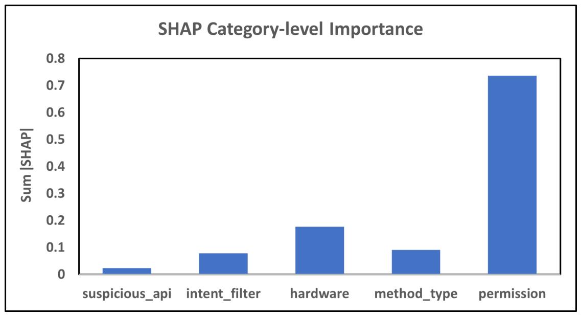
Figure 4.
Distribution of GNNExplainer explanation-subgraph sizes (number of nodes) for benign and malware applications.
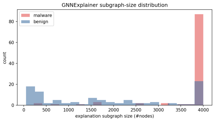
Figure 5.
GNNExplainer explanation subgraphs for (a) a correctly classified malicious and (b) a correctly classified benign application, each the application whose number of edges with mask above 0.5 is closest to the median of its class. Each panel shows the 40 highest-weighted directed edges of the explanation, all with mask values above 0.5 (self-loops included), and their endpoint nodes. Arrows show the direction of each edge, and circular arrows are self-loops. Edge colour encodes the GNNExplainer edge-mask value (colour bar; the scale spans 0.874–0.885 in (a) and 0.886–0.896 in (b)), not GAT attention scores. Node colour indicates the method type. In (a) suspicious-API nodes have a thick outline; in (b) the root node is drawn as a star. Labelled nodes are the highest-weighted hubs of separate connected components, identified by their node index in the capped graph; the root is labelled “root”. Node positions come from a force-directed layout and carry no meaning.
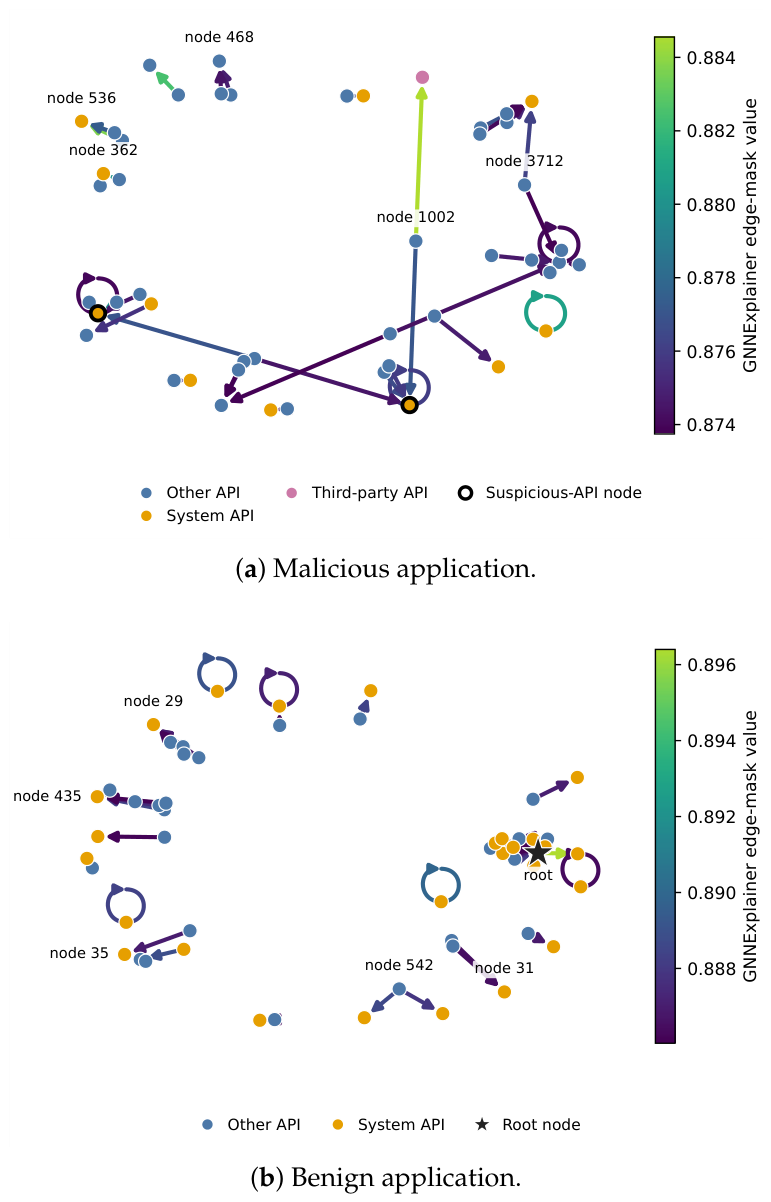
Figure 6.
Explanation-quality diagnostics on the 200-application explainability subset. (a) Comprehensiveness (left) and sufficiency (right), averaged over the 94 correctly detected malicious applications, as a function of the number k of top-ranked features deleted or kept (, the values averaged in Table 17; shaded bands: 95% bootstrap confidence intervals over applications, 2000 resamples). (b) Global importance of each of the 209 features according to SHAP (mean |SHAP value|, symmetric-logarithmic axis) and GNNExplainer (mean feature-mask value), coloured by feature category; the 115 features absent from all explained applications are grey crosses and overlap at two positions. The three features with the largest SHAP importance are labelled. Spearman is 0.211 over all 209 features and 0.124 over the 94 features present in at least one explained application.
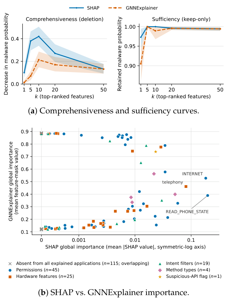
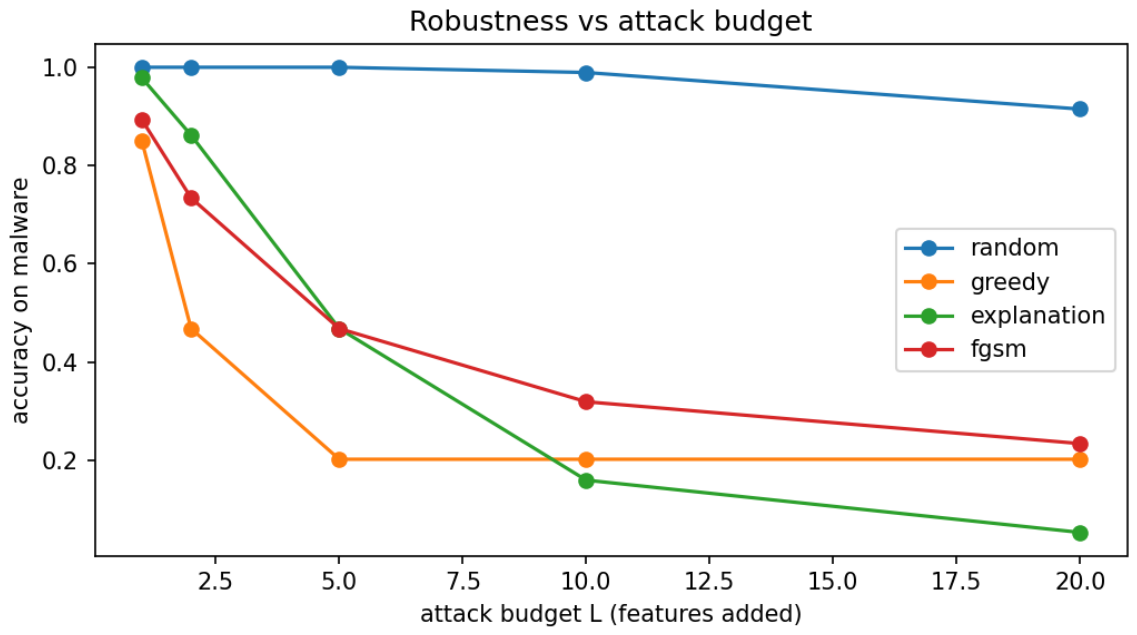
Figure 7.
Detection rate (fraction still classified as malware, i.e., 1 − evasion rate) of the 94 correctly classified malicious applications of the explainability subset as a function of the attacker’s budget L (number of added manifest features) for the four add-only attacks. The greedy attack degrades detection fastest at small budgets (15% evasion at , 53% at ) and plateaus at 80% evasion from , whereas the explanation-guided attack starts slowly (2% at ) and reaches the highest evasion (95%) at . Random additions have little effect (9% evasion at ).
Dataset Provenance, Partitioning and Evaluation Protocol
The primary dataset comprises 10,249 applications: 5243 malicious applications from the Drebin dataset [42], whose 5560 samples were collected between August 2010 and October 2012 and span 179 families, and 5006 benign applications downloaded from APKPure and the HKUST Wake Lock Misuse Detection Project [68]. To reduce the risk of mislabelled benign samples, the applications collected from the benign sources were additionally screened using VirusTotal, and samples identified as malicious were excluded from the benign set. The dataset was partitioned once, at the level of individual applications, with a fixed random seed (42). The benign and the malicious applications were shuffled separately, and the first 1000 applications of each class were held out as a balanced test set of 2000 applications. The remaining applications (4006 benign and 4243 malicious) were shuffled again within each class and divided into 80% training and 20% validation applications, which gives 6599 training and 1650 validation applications with the (slightly unbalanced) class ratio of the remaining pool. The test set was therefore kept separate from training, validation and model-selection decisions. All models in this study use this split; the reduced-protocol experiments use fixed subsets of its partitions (Table 4). Model training, model selection (on the validation partition) and the selection of the SHAP background set use no test data, and the feature vocabularies are fixed lists taken from the Android documentation that are not fitted to the data. The 200-application explainability subset was drawn from the test partition by stratified sampling with the same seed.
Because the Drebin malware set contains many repackaged near-duplicates [69], we checked for leakage between the partitions. As APK hashes are not available for all applications, we compared the extracted representations: two applications are counted as duplicates when their adjacency and node-feature matrices are identical, which is a stricter criterion than structural similarity, so the counts below are lower bounds. 710 of the 2000 test applications (35.5%; 563 benign and 147 malicious) have an identical graph representation in the training or validation partition, and 15 groups of identical representations carry conflicting labels (54 applications, mostly template-generated applications). On the 1290 test applications without a duplicate, the final model reaches 94.0% accuracy (balanced accuracy 93.0%; malware recall 96.3%, benign recall 89.7%), compared with 95.65% on the full test set and 98.6% on the 710 duplicated applications. Duplication therefore inflates the headline accuracy by about 1.6 points, and we report both figures (Section 4.2.2 and Table 11).
Because the partitioning is random at the level of individual applications, it does not take malware family, collection date, source or duplication into account. Applications of the same malware family therefore occur in both the training and the test partitions, and, as shown above, a substantial fraction of test applications has an identical representation in the training data. The reported results therefore measure in-distribution detection, which is also the protocol of the Drebin-based studies we compare with in Section 4.2.2, and they should not be read as performance on previously unseen families or on applications from later periods. Family-disjoint and time-aware evaluations are known to yield lower performance [70,71,72] and are left to future work (Section 6). The evaluation on CICMalDroid2020 (Section 4.2.3), whose applications were collected in a different period (December 2017 to December 2018) and processed with the same pipeline, partly addresses this limitation.
Each model was trained once on this split. We quantify the resulting uncertainty with 95% confidence intervals: Wilson intervals for accuracy and recall, a stratified bootstrap over the confusion matrix (20,000 resamples [73]) for precision and F1, and the Hanley–McNeil standard error for AUC [74]. For models evaluated on the full test set (2000 applications), including the final model and the branch comparison of Table 5, the half-width is about ±0.9 points for accuracy and ±0.6 points for AUC; for the reduced-protocol experiments (400 test applications) it is about ±3 points for accuracy and ±2 points for AUC. McNemar’s exact test is the procedure recommended by Dietterich [75] for comparing classifiers that can be trained only once. For the branch comparison of Table 5, the per-application predictions of all models were recomputed from the saved checkpoints on the same 2000 test applications, and we report exact McNemar tests for accuracy and DeLong tests for AUC [76], with Holm’s correction over the six hybrid-versus-branch comparisons [77]. For the reduced-protocol runs, whose per-application predictions were not retained, we report the range of McNemar p-values that is compatible with the observed confusion matrices. Two independent trainings of the same full-protocol configuration differ by 0.3 accuracy points and 0.6 AUC points (Section 4.2), which is the scale of run-to-run variation against which single-run differences should be judged.
4.2. Detection Performance
This subsection addresses RQ1. Table 5 compares XGCN-GAT with its GCN and GAT branches trained in isolation under the full protocol at three widths, and Table 6 reports paired significance tests on the same 2000 test applications. The hybrid is more accurate than the GCN branch at every width (95.70% vs. 94.20%, 96.30% vs. 94.45% and 95.95% vs. 95.05%); the difference is significant at and after Holm correction (exact McNemar test, both ), but not at (Holm ). Compared with the GAT branch, the hybrid is 0.30 and 0.10 points more accurate at and and 0.15 points less accurate at ; none of these differences is significant (), and the two models agree on 97–99% of the applications. The hybrid has the higher AUC at and , significantly only at (DeLong Holm ). This 0.55-point margin is, however, smaller than the 0.64-point difference between two trainings of the same configuration (the final model and its re-run), so we do not interpret it as an advantage of the architecture. The most consistent difference concerns missed malware: at every width the hybrid has the fewest false negatives (16, 18 and 14, compared with 30, 24 and 27 for GAT), and therefore the highest malware recall (98.2–98.6%). The earlier reduced-protocol comparison (Supplementary Table S2) shows the same qualitative picture. In answer to RQ1, fusion is therefore significantly more accurate than the GCN branch at small and medium width and on par with the stronger GAT branch, while missing the fewest malicious applications; it does not yield a significant accuracy gain over GAT.
Table 5.
Detection performance (%) of XGCN-GAT and its GCN and GAT branches trained in isolation under the full protocol (Table 4; 6599 training, 1650 validation and 2000 test applications, 1000 malicious and 1000 benign; 50 epochs; node cap 4000). Widths give the GAT per-head dimension × heads; the GCN branch has 8 times the per-head dimension. Brackets give 95% confidence intervals (accuracy: Wilson; AUC: Hanley–McNeil). Precision, recall, FN and FP refer to the malware class; F1 is macro-averaged. The final model is a separate training of the hybrid (on a different GPU) and is the model analysed in Section 4.3 and Section 4.4.
Table 6.
Paired comparison of XGCN-GAT with each branch on the same 2000 test applications. McNemar: exact two-sided test on the applications classified correctly by only one of the two models; DeLong: two-sided test for correlated AUCs; Holm: correction over the six hybrid-versus-branch comparisons. The last row compares two independent trainings of the same configuration and indicates the size of run-to-run variation.
Run-to-run variation. The configuration was trained twice under the full protocol: the final model, trained on an NVIDIA RTX 2060, reaches 95.65% accuracy, and the re-run in Table 5, trained on an NVIDIA Quadro M4000, reaches 95.95%. The two models agree on 97.6% of the test applications, and the accuracy difference is not significant (exact McNemar test, ). Such differences arise from the non-deterministic GPU scatter operations used in message passing together with the change of hardware, and they cannot be attributed to either source alone. The AUC differs more (97.82% vs. 98.46%; DeLong ), which shows that AUC differences of this size between single runs should not be interpreted as differences between architectures.
Width selection. Table 5 reports all three widths rather than a width selected on the test set. For completeness, the validation split alone, using the same validation criterion that selects the training epoch, would select for GCN, for GAT and for XGCN-GAT. At these validation-selected widths the test accuracies are 94.45%, 95.40% and 96.30%, respectively, and the hybrid is significantly more accurate than the selected GAT model (exact McNemar test, ). Because this result depends on the width selected for GAT, we report it as secondary evidence and base our conclusions on the equal-width comparisons.
XGCN-GAT is lightweight in three concrete respects. It has 0.09, 0.24 and 0.74 million trainable parameters at the three widths of Table 5 (half in each branch; 2.54 million at the width of the reduced study); the final model trains in about four minutes per epoch on the 6599 training graphs; and it classifies an application in 8–11 ms when graphs are capped at 1500 nodes (Table 7) and in about 0.1 s with the 4000-node cap of the final model, on a consumer-grade NVIDIA RTX 2060 GPU. Architecturally, it relies on a single input, the call graph, processed by two shallow branches with two message-passing layers each, whereas multi-view detectors such as DeepCatra require an additional analysis to extract call traces to critical APIs and a recurrent model over opcode sequences [27]. The reported times exclude static extraction of the call graph, which is common to all static detectors and was not included.
Table 7.
Average inference time per application for XGCN-GAT under the reduced protocol (C1–C3: GAT per-head dimension 32, 64 and 128 with 8 heads; call graphs capped at 1500 nodes; NVIDIA RTX 2060). Static graph extraction is not included.
4.2.1. Hyper-Parameter and Architecture Study
The experiments in this subsection vary one design choice at a time around the configuration under the reduced protocol (Table 4). Because they were evaluated on the same 400 test applications as the reduced-protocol capacity comparison (Supplementary Table S2), they constitute a sensitivity analysis rather than a model-selection procedure, and none of them was used to choose the configuration of the final model, which keeps the default settings. All headline results use the learning rate of 0.001 fixed a priori as the default recommended for Adam [44], even though a learning rate of 0.01 gave a higher test accuracy in this analysis (93.2%). Selecting hyper-parameters on the test split would bias the reported performance upwards [78], and the results below should therefore be interpreted only as indications of how sensitive the model is to each choice. Differences of about one percentage point (four of 400 test applications) are of the same order as the variation between two runs with identical settings (91.2% in Supplementary Table S2 and 92.2% in Table 8), and all differences in Table 8, Table 9 and Table 10 lie within the ±3-point confidence interval of a single estimate.
Learning rate, dropout, optimiser, and the overall combination strategy were varied (Table 8, Table 9 and Table 10). A learning rate of 0.01 gave the highest accuracy (93.2%) for the model, only four test applications above the default setting, and was not adopted, while dropout between 0.3 and 0.7 had little effect. Adam and AdamW performed identically and slightly ahead of AdaBelief (a difference of four test applications). The parallel-fusion design outperformed two alternative combinations: a series (stacked) hybrid and a linear-plus-softmax variant were substantially weaker (82.5% and 86.8%), differences that clearly exceed the confidence interval. Replacing the final linear layer of the trained hybrid by an SVM applied to its learned graph embeddings gave a similar accuracy (92.2%); this variant still relies on the graph representation learned by the two branches but adds a separate training stage, and we therefore retain the end-to-end softmax classifier.
Table 8.
Learning-rate sensitivity of XGCN-GAT (; reduced protocol, dropout 0.3; 400 test applications; %; F1 macro-averaged).
Table 9.
Optimiser comparison for XGCN-GAT (; reduced protocol, dropout 0.5; 400 test applications; %; F1 macro-averaged).
Table 10.
Effect of the combination strategy on detection performance (; reduced protocol, dropout 0.5; 400 test applications; %; F1 macro-averaged). “SVM classifier” replaces the final linear layer of a trained XGCN-GAT by an SVM applied to its learned graph embeddings.
4.2.2. Comparison with Recent Studies
Section 4.2 (Table 5) compared XGCN-GAT with GCN and GAT baselines under an identical protocol. This section positions it among recent published detectors (2021–2025) evaluated on Drebin, the primary dataset of this study. All values for prior work in Table 11 are quoted from the original publications and were not reproduced by us; only the XGCN-GAT row was obtained under our protocol. Each row states the data composition, input representation and evaluation protocol, so that the table provides context rather than a ranking. Where a study reports several variants, we quote its primary model.
Factors limiting direct comparability.
Data composition. Drebin distributes only malicious samples, so each study pairs it with its own benign collection. The benign sets in Table 11 range from 5000 to more than 50,000 applications, giving malware-to-benign ratios between roughly 1:1 and 1:9. Two studies also extend the malware set with samples from other sources. Identically named benchmarks therefore yield different evaluation sets.
Metrics and protocol. Under class imbalance, accuracy can remain high while F1 falls sharply. This is visible within Table 11: Yumlembam et al. [26], evaluated at a 1:9 ratio, reach the second-highest accuracy (98.7%) but an F1 of 93.1%, and the GCN variant of the same study reports 92.8% accuracy with only 63.5% F1. Metric definitions also vary, including standard versus balanced accuracy and, for F1, macro-averaged versus positive-class versus weighted averaging, which is frequently left unstated. Protocols range from a single random split to k-fold cross-validation and time-aware hold-out. We therefore base our discussion on F1 and state our averaging scheme explicitly.
Granularity of node features. This is the dominant factor among detectors with comparable graph architectures (Table 12). The highest-scoring detectors distinguish thousands of individual APIs or operate on pre-extracted feature vectors, whereas XGCN-GAT abstracts API calls into four categories derived from the method’s class path. The consequences are that system-API labels, which depend on framework class paths such as Landroid and Ljava, cannot be altered by identifier-renaming obfuscation; that every input dimension is directly interpretable, which supports the explanation analysis of Section 4.3; and that no embedding pretraining or large API vocabulary is required. The cost is some raw discriminative power, which accounts for most of the gap to the highest reported results.
Duplicate handling. None of the compared studies reports whether near-duplicate applications were removed, although Drebin is known to contain repackaged near-duplicates [69]. We find that 35.5% of our test partition has a graph representation (adjacency and node-feature matrices) identical to that of an application in the training or validation partition (Section “Dataset Provenance, Partitioning and Evaluation Protocol”). These are not necessarily duplicate files but can be distinct applications that the 209-dimensional abstraction maps to the same point; such applications are indistinguishable to any model operating on this representation. Moreover, because a two-layer message-passing network is no more discriminative than the Weisfeiler–Lehman test [79,80], graphs that are Weisfeiler–Lehman-equivalent without being identical are also indistinguishable to it, so our count of indistinguishable test applications is a lower bound. On the de-duplicated test partition accuracy is 94.0%. Since the quoted values are unlikely to have been de-duplicated, comparisons should be read against our full-partition figures, and the de-duplicated figures treated as a stricter self-assessment.
Positioning. With this caveat, the accuracy of the final XGCN-GAT model (95.65% on the full test partition, 94.0% after removing test applications whose graph representation also occurs in training) remains above the 82.7–92.8% reported by GCN detectors operating on call and API graphs (Mamdouh et al. [81]; Yumlembam et al. [26], whose single-branch GCN variant reports 92.8% accuracy, against 98.7% for the full pipeline listed in Table 11). It is comparable to the frequent-subgraph GCN of Zhao et al. [82], which reports approximately 94.4% balanced accuracy on an opcode graph rather than a call graph. Approaches that combine several views of the application, such as call-trace sequences and flow graphs [27] or graph embeddings fused with permission and intent features [26], report higher accuracies of 95.9–98.7%, and the highest reported value (99.85%) is obtained on pre-extracted static feature vectors [83] rather than on APK-level graphs. We therefore do not claim state-of-the-art accuracy, nor competitiveness on any metric whose definition differs across studies.
Table 11.
Recent detectors evaluated on Drebin malware (%). Only XGCN-GAT was obtained under our protocol; all other values are as reported by the original authors.
Judged on F1, which is the more informative metric across the differing class ratios of Table 11, XGCN-GAT (95.65%) is level with DeepCatra (95.8%) and above Yumlembam et al. (93.1%) [26], whose 1:9 class ratio costs it more than five F1 points despite the second-highest accuracy in the table. Beyond detection performance, our evaluation additionally quantifies explanation quality, which none of the compared studies reports, and adversarial robustness, which among them only Yumlembam et al. [26] also evaluate.
Table 12.
Code-level information encoded per graph node.
4.2.3. Generalisation to an Independent Dataset (CICMalDroid2020)
To assess generalisation beyond the primary dataset, we additionally evaluated XGCN-GAT and its constituent GCN and GAT models on the CICMalDroid2020 dataset [85], which contains Android applications collected between December 2017 and December 2018 from several sources. It is an independent Android malware dataset spanning four malware categories and a benign class. We used 14,158 apps in total: Adware (1502 apps), Banking (2251), Riskware (3822), and SMS malware (4788), plus 1795 benign apps. The pipeline was applied without any dataset-specific adaptation: the same extraction tool, the same 209-feature vocabulary (taken from the Android 9 documentation), and the same feature-to-node mapping were used. Features that are absent from the vocabulary, such as legacy or custom permissions, are ignored. Data are split as: 20% held out for testing; of the remaining 80%, a further 20% is used for validation and 80% for training. The models were trained from scratch on this dataset (no weights were transferred) with the fixed configuration (GCN hidden dimension 512), for 50 epochs with the Adam optimiser and a learning rate of 0.001, and without hyper-parameter tuning. Table 13 shows the results of the comparison between XGCN-GAT and the GCN and GAT models. On CICMalDroid2020, the hybrid attains the highest accuracy, F1 and AUC of the three models, 96.9% accuracy, 93.1% F1, and 98.2% AUC—a gain of 0.9 points in accuracy and 0.5 points in AUC over GAT alone, and 2.0 and 1.6 points, respectively, over GCN alone. As on Drebin, the GCN branch is the weaker of the two individually, while GAT is competitive with the hybrid. These are single runs without paired tests, and the differences between the hybrid and GAT are of the same order as the run-to-run variation observed on Drebin (Section 4.2); the ordering of the three models is nevertheless the same as on the primary dataset. The gap between accuracy and macro-F1 reflects the class imbalance of this dataset (about seven malicious applications per benign one): the benign-class recall of about 88% is the main limitation.
Table 13.
GCN vs. GAT vs. XGCN-GAT on CICMalDroid2020 (; fixed config, no hyper-parameter tuning; %; F1 macro-averaged).
Malware recall is above 96% in every category (Table 14), ranging from 96.67% for Banking to 99.79% for SMS malware. Detection is therefore not limited to a single category, which suggests that the learned graph representations capture characteristics shared across different malware behaviours.
Table 14.
Malware recall of XGCN-GAT by category on the CICMalDroid2020 test set (n: number of test applications in the category).
Although the use of a common representation across CICMalDroid2020 and the primary dataset reduces the possibility that the external results arise from dataset-specific feature engineering, the two datasets differ in their sources, collection periods, class distributions, and application populations. These differences may introduce dataset-specific characteristics that influence cross-dataset performance. Accordingly, the CICMalDroid2020 results are interpreted as an assessment of external generalisation under a fixed feature representation, rather than as evidence that dataset-specific biases are completely absent.
4.3. Explainability Analysis
This subsection addresses RQ2. The final model was explained with SHAP and GNNExplainer on the 200-application explainability subset (Table 4). On this subset, the model achieved 94.5% accuracy (95% CI 90.4–96.9%) and 98.5% AUC. Table 15 lists the ten most influential features by mean absolute SHAP value. The ranking is dominated by permission features (six of the top ten), led by two requested permissions—READ_PHONE_STATE and INTERNET; two hardware features and one method-type feature also appear in the top ten, while no suspicious-API feature is present. Aggregating attributions by category (Table 16 and Figure 3) reinforces this picture. Permission features account for the largest share of aggregate attribution by a wide margin, with hardware a distant second. The ranking changes when importance is normalised by category size (Section “Quantitative Evaluation of Explanation Quality”): the four method-type features have the highest mean per-feature attribution (0.0227), on a par with the single suspicious-API feature (0.0235) and about three times that of an average permission feature (0.0080). The mean attribution of a category with a single feature should, however, be read with caution, since it is not averaged over several features. Intent-filter features are numerous but individually weak (0.0014 per feature).
Table 15.
Top-10 globally important features by mean absolute SHAP value.
This result challenges the intuition, common in earlier graph-based studies, that API calls alone constitute the decisive signal, highlighting the contribution of Permission and Intent Filter features as well. While SHAP indicates which kinds of features drive a prediction, it cannot show where in the application the evidence resides. GNNExplainer complements it by identifying the part of the function call graph, i.e., the methods and call relations, on which the model relies. The explanation subgraph is defined as the subset of nodes and edges in the original application graph that are assigned high importance by GNNExplainer. Figure 5 illustrates this for a representative malicious and a representative benign application, selected as the applications whose explanation-subgraph size is closest to the median of their class. Across all 200 explained applications (Figure 4), malware explanation subgraphs contain many more edges than benign ones (median 30,574 vs. 7007 edges with mask value above 0.5; Mann–Whitney U test, ), and the fraction of edges retained in the explanation is higher for malware (median 0.67 vs. 0.63; ). Malware predictions are therefore supported by distributed subgraph structure rather than by isolated nodes. Two qualifications apply. The difference in absolute size largely reflects the larger call graphs of malicious applications (median 4000 vs. 1469 nodes after the node cap). Moreover, about two thirds of the edges are retained in both classes, so the explanations are broad rather than sparse and indicate over which part of the call graph the evidence is spread, rather than isolating a compact malicious signature.
4.3.1. Faithfulness, Stability, and Agreement of Explanations
This subsection addresses RQ3. The reliability of the two explainers differs markedly (Table 17). In terms of faithfulness, SHAP achieved a higher mean comprehensiveness (0.26; 95% CI 0.21–0.31) than GNNExplainer (0.12; 95% CI 0.09–0.16), indicating that removing SHAP’s top-ranked features degrades the prediction more sharply and that SHAP better identifies the features the model actually relies upon; the deletion curves are shown in Figure 6a. Both explainers have high sufficiency (0.99 and 0.98; 95% CIs 0.986–0.997 and 0.966–0.986). Conversely, GNNExplainer produced far more stable explanations, with a Spearman self-consistency of 1.00 under prediction-preserving perturbations versus 0.55 for SHAP, which partly reflects the sampling variance inherent in kernel-based Shapley estimation [53]; GNNExplainer’s stability is, however, partly an artefact of its shared mask initialisation (see below). Cross-explainer agreement was low (Spearman 0.21, Kendall’s 0.18, top-10 overlap 0.00; Spearman 0.12 over the 94 features present in the explained applications; Figure 6b), showing that the two methods emphasise substantially different features.
Figure 6a shows the faithfulness of SHAP and GNNExplainer as a function of the number k of top-ranked features, measured by comprehensiveness (decrease in malware probability when the top-k features are replaced) and sufficiency (malware probability retained when only the top-k features are kept). Both are expected to increase with k: replacing more top-ranked features removes more of the evidence the model uses, and keeping more of them brings the retained probability closer to the original 0.99. Sufficiency behaves as expected: it exceeds 0.999 at for both explainers and stays above 0.98 up to . Comprehensiveness increases at first but is non-monotonic: the decrease is largest at (0.42 for SHAP and 0.21 for GNNExplainer) and then falls back, and SHAP’s advantage is clearest at small k (0.38 vs. 0.07 at ). The later decline should not be read as the explanations becoming less faithful. The perturbation replaces features by a benign background value instead of deleting them, and because the feature matrix is normalised afterwards, replaced entries can keep contributing information, so further replacements can have non-additive effects; replacing all present features accordingly lowers the malware probability only from 0.99 to 0.86, which also confines sufficiency in our results to between 0.86 and about one. The zero-replacement analysis supports this: comprehensiveness increases with k (up to for SHAP and up to for GNNExplainer, where both reach 0.61), the probability falls to 0.39 when all present features are removed, and keeping the top five features retains about 0.98 against this baseline, so a compact set of top-ranked features suffices to preserve the decision for both explainers. SHAP’s comprehensiveness is also higher under zero replacement (0.40 vs. 0.18 at ), whereas their sufficiency differs little (0.985 vs. 0.979), so comprehensiveness is the metric that separates the explainers.
In our implementation, the feature mask of every application starts from the same seeded initialisation, and features that are absent from an application receive no gradient from the prediction, so their mask values evolve only under the regularisation terms and identically in every explanation. As a result, the 115 features that are absent from all 200 explained applications obtain identical mask values across applications and occupy the top ten positions of the global GNNExplainer ranking. This inflates GNNExplainer’s stability, which should therefore be read as an upper bound, and makes the agreement values computed over all 209 features, in particular the top-10 Jaccard index of zero, partly an artefact. Restricted to the 94 features present in at least one explained application, the Spearman correlation between the two global rankings is 0.12, a weak positive association, which confirms that the two explainers agree only weakly.
Table 17.
Quantitative evaluation of explanation quality on the explainability subset. Faithfulness: mean over of the deletion (comprehensiveness) and keep-only (sufficiency) scores (Section “Quantitative Evaluation of Explanation Quality”), computed on the 94 correctly detected malicious applications. Stability: similarity between the explanation of each of 30 malicious applications and those of 5 perturbed copies of it (Section “Quantitative Evaluation of Explanation Quality”). Agreement: similarity between the global feature rankings of the two explainers over the 200 explained applications, computed over all 209 features and over the 94 features present in at least one explained application. ↑: higher is better. * Affected by GNNExplainer’s shared mask initialisation (see text).
Taken together, these measurements caution against relying on any single explainer: SHAP is more faithful but noisier, whereas GNNExplainer is highly stable (partly by construction) but less faithful, and the two agree only weakly on which features matter most. Presenting both, and reporting their quality quantitatively, therefore gives a more honest account of model behaviour than a single explanation would.
4.3.2. Ablation Validation of the Dominant Categories
This subsection continues the answer to RQ2. Category-level ablation (Table 18) and SHAP attribution measure different notions of importance and should not be expected to produce the same ranking. Aggregate SHAP attribution quantifies how strongly the trained model’s output depends on a category and grows with the number of features it contains. Ablation, in which the detector is retrained without the category, quantifies the information that cannot be recovered from the remaining features [59,60]. Three factors explain why the rankings differ. First, category size: permissions account for 91 of the 209 features, so their aggregate attribution (0.736) is large even though their mean per-feature attribution (0.0080) is about one third of that of the four method-type features (0.0227). Second, redundancy: several permissions are almost perfectly associated with the hardware features they imply; for example, ACCESS_WIFI_STATE with android.hardware.wifi (phi coefficient 0.99 on the training data), ACCESS_FINE_LOCATION with android.hardware.location.gps (phi coefficient 0.98) and CAMERA with android.hardware.camera (phi coefficient 0.95), and permission bits are also set on the API nodes that exercise them. Shapley values distribute credit among such correlated features [86], whereas a retrained model can recover most of the removed information from the correlated ones, which limits the ablation effect of permissions (AUC 0.960 → 0.951). Third, method-type features are node-local descriptors present on every method node and summarise the composition of the call graph (system, third-party, component and other methods). This information is not available in the manifest and cannot be reconstructed from the remaining categories, which is consistent with method-type removal causing the largest AUC reduction (0.960 → 0.933). The row “Drop top-10 SHAP features” supports this reading: removing the ten individually most important features, which span four categories, reduces the AUC by 1.5 points, more than removing all 91 permission features.
Table 18.
Category-level ablation results. Each model is retrained without the category for five epochs on 1000 training applications and evaluated on 400 validation applications (202 malicious, 198 benign); F1 refers to the malware class. 95% confidence half-widths are about ±0.03 for accuracy and ±0.02 for AUC.
These differences should be interpreted with the uncertainty of the ablation evaluation in mind. Each ablated model was retrained for five epochs on 1000 training applications and evaluated on 400 validation applications; the 95% confidence interval of each accuracy estimate is therefore about ±3 points and that of each AUC about ±2 points. All accuracy differences in Table 18 (at most 1.0 point) fall within sampling uncertainty, and among the AUC differences only the reduction caused by removing method-type features (2.7 points) exceeds the half-width of a single estimate. The small AUC increase after removing hardware features (+0.4 points) should likewise not be interpreted as a real improvement.
4.4. Adversarial Robustness
This subsection addresses RQ4. Only malware that the model detects is attacked, because an application that is already misclassified as benign requires no perturbation. The attacks are therefore applied to the 94 malicious applications of the explainability subset that the final model classifies correctly (Table 4), and the evasion rate is the fraction of these applications that is classified as benign after the perturbation. The robustness analysis reveals a genuine but bounded feature-space vulnerability under the defined add-only threat model (Table 19 and Figure 7). The greedy attacker evades detection on only 15% of correctly classified malware at a budget of , rising to a ceiling of 80% by that further budget does not improve, at a mean cost of 2.25 added features among successful evasions. The explanation-guided attack is less efficient at very small budgets (2% evasion at ) but ultimately reaches the highest evasion rate of any attack tested—95% at , at a mean cost of 5.96 features—demonstrating that the attributions used to interpret the model also reveal a viable, though not the cheapest, path to evade it. Explanation-guided perturbations require no model queries during the attack once feature attributions are available; in our experiments these attributions were computed with full model access, but a deployment that exposes explanations to users would provide them to an attacker at no additional cost, in line with earlier findings that explanations can guide attacks on malware classifiers [37]. The gradient-based (FGSM) attack is less effective, reaching 77% evasion by . The random baseline is considerably less effective throughout the tested budget range, achieving only 9% evasion at and requiring about 15 added features on average among successful attacks. No attack therefore evades detection reliably with a single added feature: at the evasion rate is 15% for the greedy attack and 2% for the explanation-guided attack; detection degrades substantially only at budgets of two to five features for the greedy attack and of five or more features for the explanation-guided attack.
Table 19.
Evasion rate of the 94 correctly classified malicious applications of the explainability subset and mean perturbation size by attack and budget L, with the attacker knowledge assumed by each attack [63]. Mean features needed are averaged over successfully evaded samples only; since the attacks succeed on different samples, these means are not directly comparable across attacks.
Table 20 lists the features most frequently added by the explanation-guided attack. Three are normal-protection permissions, four are dangerous permissions, two of which (SEND_SMS and READ_SMS) belong to the restricted SMS permission group, and three are hardware features. In terms of the feasibility analysis of Section 3.4 (Table 3), two of the three most frequently added features are therefore among the hardest to add to an application distributed through Google Play.
To assess a simple defence, a model with the same architecture was retrained from scratch for three epochs on 800 training applications, in which 200 correctly detected malicious applications were replaced by greedily perturbed copies (up to added features) that kept their malicious label. Both the undefended final model and the retrained model were then attacked with the greedy attack at on 60 of the 94 malicious applications of Table 19, none of which was used for retraining (Table 21). For computational reasons, this experiment used a version of the greedy attack that evaluates at most 60 candidate features per application. On these 60 applications, the greedy evasion rate is 75.0% (45/60) for the undefended model and 71.7% (43/60) for the retrained model. The difference corresponds to two applications and is not statistically significant (exact McNemar test, ). Evaluated on the full 2000-application test partition without perturbation, the retrained model attains 91.40% accuracy and 96.47% AUC. To establish how much of the difference from the final model is attributable to the augmentation rather than to the reduced training protocol, we trained an additional model with the same architecture under the identical reduced protocol—800 training applications, three epochs, same seed and data order—but without augmentation; it attains 91.55% accuracy and 96.71% AUC on the same clean partition. The augmentation therefore accounts for 0.15 percentage points of accuracy and 0.24 points of AUC, a difference of three applications out of 2000, while the remaining 4.10 points of accuracy separating the retrained model from the final model are attributable to the reduced training data and epoch count alone. Replacing a quarter of the malicious training applications with greedily perturbed copies thus leaves clean detection essentially unchanged and causes no degradation on unperturbed samples. Because the retrained model also used far fewer training data and epochs than the final model, this comparison is only indicative. Naive augmentation with pre-computed adversarial examples therefore yields no measurable improvement in robustness. The undefended evasion rate in this experiment (75%) differs from the 80% reported in Table 19 because it was measured on a subset of 60 applications and with the candidate-limited greedy attack. More principled approaches, such as adversarial training with attacks generated during training [87,88] or monotonic classifiers [89], may therefore be needed to address the vulnerability. We report this finding explicitly because it highlights an important open problem rather than suggesting that the robustness issue has been resolved.
Table 20.
Features most frequently added by the explanation-guided attack: number of the 94 attacked applications in which the feature is among the first five additions. The ranking is global (mean signed SHAP value over the 200 explained applications), restricted in each application to the permission and hardware features it does not already declare.
Table 21.
Greedy evasion at of the undefended final model and the adversarially retrained model on the same 60 malicious applications (candidate-limited greedy attack), and clean accuracy and AUC (%) on the complete test partition of 2000 applications without perturbation.
5. Discussion
In summary, the four research questions are answered as follows. RQ1: under an identical protocol, parallel fusion is significantly more accurate than the GCN branch at two of three widths, on par with the GAT branch, and misses the fewest malicious applications; a similar ordering is observed on CICMalDroid2020. RQ2: permission features dominate aggregate SHAP attribution, whereas method-type features carry the largest per-feature attribution of any multi-feature category and the only clear ablation effect; the two notions of importance are complementary. RQ3: SHAP is more faithful than GNNExplainer, GNNExplainer’s near-perfect stability is partly an artefact of its mask initialisation, and the two explainers agree only weakly. RQ4: under the add-only, feature-space threat model, greedy and explanation-guided attacks evade 80% and 95% of correctly detected malware at a budget of 20 features, and naive adversarial retraining yields no measurable improvement.
The results paint a nuanced picture that is directly relevant to the deployment of graph-based detectors in privacy- and security-sensitive settings. On the detection axis, the parallel fusion of graph convolution and graph attention delivers 95.65% accuracy and 97.8% AUC for the final model on a held-out test set of 2000 applications, improves significantly on the GCN branch but not on the GAT branch, while remaining efficient enough to run on commodity hardware. This confirms the practical value of the architecture but also situates it honestly: the hybrid is a solid, efficient detector rather than a state-of-the-art-beating one (Section 4.2.2), and its principal contribution lies in the transparency and robustness analysis layered on top.
On the transparency axis, the explainability findings carry two lessons. First, the permission category has the largest aggregate SHAP attribution, consistent with prior research showing that permissions declared in the Android manifest can provide strong discriminatory information for malware detection [90]. However, the method-type category—a structural property associated with individual API calls rather than a manifest-derived feature—exhibits a substantially higher per-feature attribution and produces the largest ablation effect. Because aggregate attribution grows with category size and is shared among correlated features, whereas the ablation effect measures information that cannot be recovered from the remaining categories, these findings are complementary rather than contradictory (Section 4.3.2). This indicates that the model’s discriminative signal is not derived solely from manifest-level information, but also from the structural and semantic characteristics of the function call graph. Second, and more cautionary, the explanations are not interchangeable: SHAP is more faithful yet noisier, GNNExplainer is more stable (partly by construction) yet less faithful, and the two agree only weakly on which features matter. Reporting explanation quality quantitatively, as done here, is therefore not a formality but a prerequisite for trusting any single explanation in an operational security workflow.
The explanations reported in this study are post hoc approximations of the model’s input–output behaviour, not causal accounts of maliciousness. SHAP values quantify how the model’s output changes when features are replaced by background values, which is an interventional query on the model rather than on the application [91]. GNNExplainer’s masks are the solution of a regularised optimisation problem whose sparsity and entropy penalties shape the result. Neither method establishes that a feature causes an application to be malicious, or even that the model relies on it in a unique way [92]. The low agreement between the two explainers (Spearman over all 209 features and 0.124 over the 94 features present in the explained applications) should be read in this light. Such disagreement has been observed across models and data modalities [93], and here it partly reflects the different questions the methods answer: SHAP distributes the output difference relative to a benign reference among feature types, whereas GNNExplainer searches for a sparse mask that preserves the prediction.
The combination of near-perfect stability and low comprehensiveness observed for GNNExplainer also warrants caution, because stability alone can be achieved by explanations that depend little on the input [94]. In our implementation this concern applies directly: all explanations start from the same mask initialisation, so features absent from an application evolve identically in every explanation, which inflates GNNExplainer’s stability and distorts rank agreement computed over all features (Section 4.3.1). For operational use, we therefore recommend treating explanations as hypotheses to be checked, for example through targeted ablation as in Section 4.3.2, and using more than one explainer, in line with earlier evaluations of explanation methods in security [23,24] and with arguments for inherently interpretable models in high-stakes settings [95].
From a robustness perspective, the results show that strong benchmark performance does not necessarily translate into strong resistance to adversarial attack. Under the considered add-only threat model, the greedy attack achieves successful evasion with an average of only 2.25 added features, but its effectiveness plateaus at 80%, leaving a substantial fraction of malware samples resistant to this attack. The explanation-guided attack is less feature-efficient than greedy search, yet ultimately achieves a higher evasion rate, reaching 95% at , and requires no model queries during the attack once feature attributions are available (in our experiments, these were computed with full model access). This result highlights an important connection between interpretability and robustness: the same feature attributions used to explain the detector can also provide useful guidance for constructing evasive perturbations. Consequently, explanations may have security implications when exposed alongside a deployed detector, and robustness should be considered alongside predictive performance and interpretability during model design. Finally, naive adversarial retraining produced no measurable improvement (75.0% vs. 71.7% greedy evasion at on 60 malicious test applications, a difference of two applications). This suggests that the observed vulnerability cannot be addressed through straightforward data augmentation alone and may require more targeted defences. All robustness results refer to feature-space perturbations of manifest declarations: they establish a vulnerability of the detector, not end-to-end evasion of deployed detection pipelines, which depends on problem-space constraints (Section 3.4) that were not evaluated here.
Limitations. The representation abstracts method identities into four method types and a suspicious-API flag, symmetrises call edges, restricts large graphs to their highest-degree nodes and summarises the graph by mean pooling, so information such as specific API names, call direction, call order and the periphery of very large call graphs is not available to the model. A structure-free logistic regression on the application-level presence of the same 209 features reaches 92.2% accuracy and 97.2% AUC on the test set, compared with 95.65% and 97.8% for the final model (an SVM on mean-pooled node features, which dilutes the manifest features by the graph size, reaches only 81.8%). The call-graph structure thus adds about 3.5 accuracy points over a strong flat baseline at a similar AUC. Together with the consistent difference between the GCN and GAT branches, which receive identical features, and the effect of removing the node-local method-type features, this indicates that structural information is used, although most of the discriminative signal is present in the features themselves. The effect of the node cap was not quantified. Richer node attributes (e.g., API embeddings), uncapped training and hierarchical pooling are left to future work. Limitations of the evaluation protocol, in particular the in-distribution nature of the random split and the duplicated representations across partitions, are discussed in Section “Dataset Provenance, Partitioning and Evaluation Protocol”.
6. Future Work
Several directions follow from the limitations of this study. First, the robustness results should be validated in the problem space by rebuilding perturbed APKs, re-extracting their graphs and testing them against complete detection pipelines [34], and extended to attacks that modify the call graph itself [35,36]. Second, the finding that naive augmentation does not improve robustness, while greedy and explanation-guided attacks evade 80–95% of malware under the add-only model, calls for stronger defences, such as adversarial training with attacks generated during training [87,88] or monotonic classifiers that cannot be evaded by adding features [89]. Third, detection should be evaluated under family-disjoint and time-aware splits [71] and at realistic class ratios. Fourth, the explanation analysis should be extended to further GNN explainers, such as PGExplainer and SubgraphX [49,50], and the role of the root node should be assessed by ablation.
7. Conclusions
This paper presented XGCN-GAT, a hybrid graph neural network for static Android malware detection that fuses graph convolutional and graph attention branches over function call graphs, together with a quantitative evaluation of its explanations and of its robustness to feature-space evasion. On a Drebin-based dataset of 10,249 applications, the final model attained 95.65% accuracy and 97.8% AUC on a held-out test set of 2000 applications (94.0% accuracy on the test applications without a duplicate in the training data). In a controlled comparison with its branches under the same protocol and at three model widths, the hybrid was significantly more accurate than the GCN branch at two widths, was on par with the GAT branch, and missed the fewest malicious applications at every width; differences in AUC between the hybrid and GAT were of the same order as the variation between two trainings of the same model. A similar ordering was observed on CICMalDroid2020 (96.9% accuracy, 93.1% macro-F1, 98.2% AUC), where the benign-class recall (about 88%) remains the main limitation.
The explainability analysis showed that permission features carry the largest aggregate SHAP attribution, largely because the category is large, whereas method-type features carry the largest per-feature attribution of any multi-feature category and are the only category whose removal clearly reduced the AUC. These are complementary notions of importance rather than contradictory findings. SHAP was more faithful than GNNExplainer, whose near-perfect stability proved to be partly an artefact of its shared mask initialisation, and the two explainers agreed only weakly in their feature rankings. This argues against relying on any single post hoc explainer, and all explanations reported here should be read as approximations of model behaviour rather than causal accounts.
Under a feature-space, add-only threat model restricted to manifest-level permissions and hardware features, a small number of added features evaded detection for a large proportion of correctly classified malware: up to 80% for greedy search and 95% for explanation-guided perturbations at a budget of 20 features. Naive adversarial retraining produced no measurable improvement. These results establish a feature-space vulnerability of the detector; whether they translate into evasion of complete, deployed detection pipelines depends on problem-space constraints that were not evaluated here. By reporting these limitations explicitly, this study provides a reproducible baseline for more transparent and robust graph-based malware detectors.
Supplementary Materials
The following supporting information can be downloaded at https://www.mdpi.com/article/10.3390/jcp6050180/s1, Table S1: Complete list of the 209 node features with index, category and Android protection level (permissions); Table S2: Capacity comparison of GCN, GAT and XGCN-GAT under the reduced protocol (C1–C3), with 95% confidence intervals and McNemar bounds.
Author Contributions
Conceptualisation, methodology, and writing were carried out by the authors. All authors have read and agreed to the published version of the manuscript.
Funding
This research received no external funding.
Data Availability Statement
The source code, feature-extraction scripts, the complete 209-feature vocabulary and feature-to-node mapping, the identifiers and train/validation/test split indices of all applications, training configurations and random seeds, trained model checkpoints, the explainability and explanation-quality evaluation scripts, and the attack-generation and adversarial-retraining scripts will be made publicly available in a GitHub repository, archived on Zenodo with a persistent DOI, upon publication. The APK files are not redistributed; the malicious applications can be obtained from the Drebin authors, the benign applications from APKPure and the HKUST Wake Lock Misuse Detection Project using the published identifiers, and the CICMalDroid2020 applications from the Canadian Institute for Cybersecurity.
Conflicts of Interest
The authors declare no conflicts of interest.
References
- Goel, A.; Sahil, G. Growth of Mobile Applications and the Rise of Privacy Issues. Int. J. Electron. Financ. 2024, 13, 20–35. [Google Scholar] [CrossRef] [Scilit]
- Xun, J.; Chong, W.K.; Dolega, L. Mobile Operating Systems’ Impact on Customer Value: IOS vs. Android. J. Comput. Inf. Syst. 2025, 65, 401–414. [Google Scholar] [CrossRef] [Scilit]
- Ferdous, J.; Islam, R.; Mahboubi, A.; Islam, M.Z. A Review of State-of-the-Art Malware Attack Trends and Defense Mechanisms. IEEE Access 2023, 11, 121118–121141. [Google Scholar] [CrossRef] [Scilit]
- Liu, Y.; Tantithamthavorn, C.; Li, L.; Liu, Y. Deep Learning for Android Malware Defenses: A Systematic Literature Review. ACM Comput. Surv. 2022, 55, 1–36. [Google Scholar] [CrossRef] [Scilit]
- Suo, D.; Xue, L.; Huang, W.; Tan, R.; Sun, G. Assessing the Capability of Android Dynamic Analysis Tools to Combat Anti-Runtime Analysis Techniques. J. Syst. Softw. 2025, 234, 112747. [Google Scholar] [CrossRef] [Scilit]
- Papankar, P.; Mandaogade, N. Advancements in Android Malware Detection: A Comprehensive Review of Graph Neural Network Approaches. Int. J. Adv. Res. Comput. Sci. Manag. Stud. 2024, 12, 13–19. [Google Scholar] [CrossRef] [Scilit]
- Zhang, D.; Wu, X.; He, E.; Guo, X.; Yang, X.; Li, R.; Li, H. Android Malware Detection Based on Hypergraph Neural Networks. Appl. Sci. 2023, 13, 12629. [Google Scholar] [CrossRef] [Scilit]
- Kipf, T.N.; Welling, M. Semi-Supervised Classification with Graph Convolutional Networks. In Proceedings of the 5th International Conference on Learning Representations (ICLR); ICLR: Toulon, France, 2017. [Google Scholar]
- Gao, H.; Cheng, S.; Zhang, W. GDroid: Android Malware Detection and Classification with Graph Convolutional Network. Comput. Secur. 2021, 106, 102264. [Google Scholar] [CrossRef] [Scilit]
- Lu, X.; Zhao, J.; Zhu, S.; Lio, P. SNDGCN: Robust Android Malware Detection Based on Subgraph Network and Denoising GCN Network. Expert Syst. Appl. 2024, 250, 123922. [Google Scholar] [CrossRef] [Scilit]
- Zaidi, S.H.; Fuzail, M.; Raza, A.; Aziz, Y.; Abid, M.K.; Aslam, N. A Deep Learning Framework Based on GCN Model for Android Malware Detection. J. Comput. Biomed. Inform. 2024, 7, 484–500. [Google Scholar]
- Veličković, P.; Cucurull, G.; Casanova, A.; Romero, A.; Liò, P.; Bengio, Y. Graph Attention Networks. In Proceedings of the 6th International Conference on Learning Representations (ICLR); ICLR: Vancouver, BC, Canada, 2018. [Google Scholar]
- Sun, C.; Li, C.; Lin, X.; Zheng, T.; Meng, F.; Rui, X.; Wang, Z. Attention-Based Graph Neural Networks: A Survey. arXiv 2026, arXiv:2605.08679. [Google Scholar]
- Dang, Q.V. HeteroMalGAT: A Heterogeneous Graph Attention Network Framework for Android Malware Detection via Knowledge Graph Representations. In Proceedings of the International Conference on Future Data and Security Engineering; Springer: Singapore, 2025; pp. 128–142. [Google Scholar]
- Fan, C.-I.; Lu, S.-F.; Shie, C.-H.; Tsai, M.-F.; Morikawa, T.; Takahashi, T.; Ban, T. A Graph-Based Interpretable Framework for Effective Android Malware Detection. Comput. Model. Eng. Sci. 2026, 147, 47. [Google Scholar] [CrossRef] [Scilit]
- Bilot, T.; El Madhoun, N.; Al Agha, K.; Zouaoui, A. A Survey on Malware Detection with Graph Representation Learning. ACM Comput. Surv. 2024, 56, 1–36. [Google Scholar] [CrossRef] [Scilit]
- Lundberg, S.M.; Lee, S.I. A Unified Approach to Interpreting Model Predictions. In Proceedings of the Advances in Neural Information Processing Systems 30 (NeurIPS); Curran Associates, Inc.: Red Hook, NY, USA, 2017; pp. 4765–4774. [Google Scholar]
- Ying, R.; Bourgeois, D.; You, J.; Zitnik, M.; Leskovec, J. GNNExplainer: Generating Explanations for Graph Neural Networks. In Proceedings of the Advances in Neural Information Processing Systems 32 (NeurIPS); Curran Associates, Inc.: Red Hook, NY, USA, 2019. [Google Scholar]
- Chen, Y.H.; Lin, S.C.; Huang, S.C.; Lei, C.L.; Huang, C.Y. Guided Malware Sample Analysis Based on Graph Neural Networks. IEEE Trans. Inf. Forensics Secur. 2023, 18, 4128–4143. [Google Scholar] [CrossRef] [Scilit]
- Bui, T.C. Enhancing Explainability of Graph Neural Networks Through Conceptual and Structural Analyses and Their Extensions. arXiv 2025, arXiv:2512.08344. [Google Scholar]
- Luša, R.; Pintar, D.; Vranić, M. TE-G-SAGE: Explainable Edge-Aware Graph Neural Networks for Network Intrusion Detection. Modelling 2025, 6, 165. [Google Scholar] [CrossRef] [Scilit]
- Mohammadian, H.; Higgins, G.; Ansong, S.; Razavi-Far, R.; Ghorbani, A.A. Explainable Malware Detection Through Integrated Graph Reduction and Learning Techniques. Big Data Res. 2025, 41, 100555. [Google Scholar] [CrossRef] [Scilit]
- Warnecke, A.; Arp, D.; Wressnegger, C.; Rieck, K. Evaluating Explanation Methods for Deep Learning in Security. In Proceedings of the IEEE European Symposium on Security and Privacy (EuroS&P); IEEE: New York, NY, USA, 2020; pp. 158–174. [Google Scholar]
- Fan, M.; Wei, W.; Xie, X.; Liu, Y.; Guan, X.; Liu, T. Can We Trust Your Explanations? Sanity Checks for Interpreters in Android Malware Analysis. IEEE Trans. Inf. Forensics Secur. 2021, 16, 838–853. [Google Scholar] [CrossRef] [Scilit]
- Chandrika, G.N.; Reddy, E.S. Graph Classification System Using Normalised Graph Convolutional Networks. Int. J. Syst. Syst. Eng. 2021, 11, 320–335. [Google Scholar] [CrossRef] [Scilit]
- Yumlembam, R.; Issac, B.; Jacob, S.M.; Yang, L. IoT-based Android Malware Detection Using Graph Neural Network with Adversarial Defense. IEEE Internet Things J. 2023, 10, 8432–8444. [Google Scholar] [CrossRef] [Scilit]
- Wu, Y.; Shi, J.; Wang, P.; Zeng, D.; Sun, C. DeepCatra: Learning Flow- and Graph-Based Behaviours for Android Malware Detection. IET Inf. Secur. 2023, 17, 118–130. [Google Scholar] [CrossRef] [Scilit]
- Li, M.; Sun, H.; Huang, Y.; Chen, H. Shapley Value: From Cooperative Game to Explainable Artificial Intelligence. Auton. Intell. Syst. 2024, 4, 2. [Google Scholar] [CrossRef] [Scilit]
- Li, Y.; Zhou, J.; Verma, S.; Chen, F. A Survey of Explainable Graph Neural Networks: Taxonomy and Evaluation Metrics. arXiv 2022, arXiv:2207.12599. [Google Scholar]
- Yuan, H.; Yu, H.; Gui, S.; Ji, S. Explainability in Graph Neural Networks: A Taxonomic Survey. IEEE Trans. Pattern Anal. Mach. Intell. 2023, 45, 5782–5799. [Google Scholar] [CrossRef] [Scilit] [PubMed]
- Agarwal, C.; Queen, O.; Lakkaraju, H.; Zitnik, M. Evaluating Explainability for Graph Neural Networks. Sci. Data 2023, 10, 144. [Google Scholar] [CrossRef] [Scilit] [PubMed]
- Grosse, K.; Papernot, N.; Manoharan, P.; Backes, M.; McDaniel, P. Adversarial Examples for Malware Detection. In Proceedings of the Computer Security—ESORICS 2017; Lecture Notes in Computer Science; Springer: Cham, Switzerland, 2017; Volume 10493, pp. 62–79. [Google Scholar]
- Demontis, A.; Melis, M.; Biggio, B.; Maiorca, D.; Arp, D.; Rieck, K.; Corona, I.; Giacinto, G.; Roli, F. Yes, Machine Learning Can Be More Secure! A Case Study on Android Malware Detection. IEEE Trans. Dependable Secur. Comput. 2019, 16, 711–724. [Google Scholar] [CrossRef] [Scilit]
- Pierazzi, F.; Pendlebury, F.; Cortellazzi, J.; Cavallaro, L. Intriguing Properties of Adversarial ML Attacks in the Problem Space. In Proceedings of the IEEE Symposium on Security and Privacy (S&P); IEEE: New York, NY, USA, 2020; pp. 1332–1349. [Google Scholar]
- Zhao, K.; Zhou, H.; Zhu, Y.; Zhan, X.; Zhou, K.; Li, J.; Yu, L.; Yuan, W.; Luo, X. Structural Attack against Graph Based Android Malware Detection. In Proceedings of the ACM SIGSAC Conference on Computer and Communications Security (CCS); ACM: New York, NY, USA, 2021; pp. 3218–3235. [Google Scholar]
- Li, H.; Cheng, Z.; Wu, B.; Yuan, L.; Gao, C.; Yuan, W.; Luo, X. Black-box Adversarial Example Attack towards FCG Based Android Malware Detection under Incomplete Feature Information. In Proceedings of the 32nd USENIX Security Symposium; USENIX Association: Berkeley, CA, USA, 2023. [Google Scholar]
- Severi, G.; Meyer, J.; Coull, S.; Oprea, A. Explanation-Guided Backdoor Poisoning Attacks Against Malware Classifiers. In Proceedings of the 30th USENIX Security Symposium; USENIX Association: Berkeley, CA, USA, 2021; pp. 1487–1504. [Google Scholar]
- Desnos, A. Androguard: Reverse Engineering, Malware and Goodware Analysis of Android Applications. Software Project. 2026. Available online: https://github.com/androguard/androguard (accessed on 11 October 2026).
- Li, L.; Bissyandé, T.F.; Papadakis, M.; Rasthofer, S.; Bartel, A.; Octeau, D.; Klein, J.; Le Traon, Y. Static analysis of android apps: A systematic literature review. Inf. Softw. Technol. 2017, 88, 67–95. [Google Scholar] [CrossRef] [Scilit]
- Gascon, H.; Yamaguchi, F.; Arp, D.; Rieck, K. Structural Detection of Android Malware using Embedded Call Graphs. In Proceedings of the 2013 ACM Workshop on Artificial Intelligence and Security (AISec); ACM: New York, NY, USA, 2013; pp. 45–54. [Google Scholar]
- Au, K.W.Y.; Zhou, Y.F.; Huang, Z.; Lie, D. Pscout: Analyzing the android permission specification. In Proceedings of the 2012 ACM Conference on Computer and Communications Security; ACM: New York, NY, USA, 2012; pp. 217–228. [Google Scholar]
- Arp, D.; Spreitzenbarth, M.; Hübner, M.; Gascon, H.; Rieck, K. Drebin: Effective and Explainable Detection of Android Malware in Your Pocket. In Proceedings of the Network and Distributed System Security Symposium (NDSS); Internet Society: Reston, VA, USA, 2014. [Google Scholar]
- Zhu, R.; Li, C.; Niu, D.; Zhang, H.; Kinawi, H. Android Malware Detection Using Large-Scale Network Representation Learning. arXiv 2018, arXiv:1806.04847. [Google Scholar]
- Kingma, D.P.; Ba, J. Adam: A Method for Stochastic Optimization. In Proceedings of the 3rd International Conference on Learning Representations (ICLR); ICLR: San Diego, CA, USA, 2015. [Google Scholar]
- Gilmer, J.; Schoenholz, S.S.; Riley, P.F.; Vinyals, O.; Dahl, G.E. Neural Message Passing for Quantum Chemistry. In Proceedings of the 34th International Conference on Machine Learning (ICML); PMLR: Sydney, Australia, 2017; Volume 70, pp. 1263–1272. [Google Scholar]
- Hu, W.; Fey, M.; Zitnik, M.; Dong, Y.; Ren, H.; Liu, B.; Catasta, M.; Leskovec, J. Open Graph Benchmark: Datasets for Machine Learning on Graphs. In Proceedings of the Advances in Neural Information Processing Systems 33 (NeurIPS); Curran Associates, Inc.: Red Hook, NY, USA, 2020; pp. 22118–22133. [Google Scholar]
- Cai, C.; Hy, T.S.; Yu, R.; Wang, Y. On the Connection Between MPNN and Graph Transformer. In Proceedings of the 40th International Conference on Machine Learning (ICML); PMLR: Honolulu, HI, USA, 2023; Volume 202. [Google Scholar]
- Li, Q.; Han, Z.; Wu, X.M. Deeper Insights into Graph Convolutional Networks for Semi-Supervised Learning. In Proceedings of the AAAI Conference on Artificial Intelligence; AAAI: Palo Alto, CA, USA, 2018; Volume 32, pp. 3538–3545. [Google Scholar]
- Luo, D.; Cheng, W.; Xu, D.; Yu, W.; Zong, B.; Chen, H.; Zhang, X. Parameterized Explainer for Graph Neural Network. In Proceedings of the Advances in Neural Information Processing Systems 33 (NeurIPS); Curran Associates, Inc.: Red Hook, NY, USA, 2020; pp. 19620–19631. [Google Scholar]
- Yuan, H.; Yu, H.; Wang, J.; Li, K.; Ji, S. On Explainability of Graph Neural Networks via Subgraph Explorations. In Proceedings of the 38th International Conference on Machine Learning (ICML); PMLR: Virtual, 2021; Volume 139, pp. 12241–12252. [Google Scholar]
- Sundararajan, M.; Taly, A.; Yan, Q. Axiomatic Attribution for Deep Networks. In Proceedings of the 34th International Conference on Machine Learning (ICML); PMLR: Sydney, Australia, 2017; Volume 70, pp. 3319–3328. [Google Scholar]
- Sundararajan, M.; Najmi, A. The Many Shapley Values for Model Explanation. In Proceedings of the 37th International Conference on Machine Learning (ICML); PMLR: Virtual, 2020; Volume 119, pp. 9269–9278. [Google Scholar]
- Covert, I.; Lee, S.I. Improving KernelSHAP: Practical Shapley Value Estimation Using Linear Regression. In Proceedings of the 24th International Conference on Artificial Intelligence and Statistics (AISTATS); PMLR: Virtual, 2021; Volume 130, pp. 3457–3465. [Google Scholar]
- DeYoung, J.; Jain, S.; Rajani, N.F.; Lehman, E.; Xiong, C.; Socher, R.; Wallace, B.C. ERASER: A Benchmark to Evaluate Rationalized NLP Models. In Proceedings of the 58th Annual Meeting of the Association for Computational Linguistics (ACL); Association for Computational Linguistics: Stroudsburg, PA, USA, 2020; pp. 4443–4458. [Google Scholar]
- Dasgupta, S.; Frost, N.; Moshkovitz, M. Framework for evaluating faithfulness of local explanations. In Proceedings of the 39th International Conference on Machine Learning; PMLR: Baltimore, MD, USA, 2022; Volume 162, pp. 4794–4815. [Google Scholar]
- Spearman, C. The Proof and Measurement of Association between Two Things. Am. J. Psychol. 1904, 15, 72–101. [Google Scholar] [CrossRef] [Scilit] [PubMed]
- Jaccard, P. The Distribution of the Flora in the Alpine Zone. New Phytol. 1912, 11, 37–50. [Google Scholar] [CrossRef] [Scilit]
- Kendall, M.G. A New Measure of Rank Correlation. Biometrika 1938, 30, 81–93. [Google Scholar] [CrossRef] [Scilit]
- Covert, I.; Lundberg, S.; Lee, S.I. Explaining by Removing: A Unified Framework for Model Explanation. J. Mach. Learn. Res. 2021, 22, 1–90. [Google Scholar]
- Hooker, S.; Erhan, D.; Kindermans, P.J.; Kim, B. A Benchmark for Interpretability Methods in Deep Neural Networks. In Proceedings of the Advances in Neural Information Processing Systems 32 (NeurIPS); Curran Associates, Inc.: Red Hook, NY, USA, 2019. [Google Scholar]
- Covert, I.; Lundberg, S.M.; Lee, S.I. Understanding Global Feature Contributions with Additive Importance Measures. In Proceedings of the Advances in Neural Information Processing Systems 33 (NeurIPS); Curran Associates, Inc.: Red Hook, NY, USA, 2020; pp. 17212–17223. [Google Scholar]
- Goodfellow, I.J.; Shlens, J.; Szegedy, C. Explaining and Harnessing Adversarial Examples. In Proceedings of the 3rd International Conference on Learning Representations (ICLR); ICLR: San Diego, CA, USA, 2015. [Google Scholar]
- Biggio, B.; Roli, F. Wild Patterns: Ten Years After the Rise of Adversarial Machine Learning. Pattern Recognit. 2018, 84, 317–331. [Google Scholar] [CrossRef] [Scilit]
- Android Developers. Permissions on Android. Available online: https://developer.android.com/guide/topics/permissions/overview (accessed on 11 October 2026).
- Felt, A.P.; Chin, E.; Hanna, S.; Song, D.; Wagner, D. Android Permissions Demystified. In Proceedings of the 18th ACM Conference on Computer and Communications Security (CCS); ACM: New York, NY, USA, 2011; pp. 627–638. [Google Scholar]
- Google Play Console Help. Use of SMS or Call Log Permission Groups. Available online: https://support.google.com/googleplay/android-developer/ (accessed on 11 October 2026).
- Android Developers. <uses-feature> Element. Available online: https://developer.android.com/guide/topics/manifest/uses-feature-element (accessed on 11 October 2026).
- Liu, Y.; Xu, C.; Cheung, S.C.; Terragni, V. Understanding and Detecting Wake Lock Misuses for Android Applications. In Proceedings of the 24th ACM SIGSOFT International Symposium on the Foundations of Software Engineering (FSE); ACM: New York, NY, USA, 2016; pp. 396–409. [Google Scholar]
- Irolla, P.; Dey, A. The Duplication Issue within the Drebin Dataset. J. Comput. Virol. Hacking Tech. 2018, 14, 245–249. [Google Scholar] [CrossRef] [Scilit]
- Allix, K.; Bissyandé, T.F.; Klein, J.; Le Traon, Y. Are Your Training Datasets Yet Relevant? An Investigation into the Importance of Timeline in Machine Learning-Based Malware Detection. In Proceedings of the International Symposium on Engineering Secure Software and Systems (ESSoS); Lecture Notes in Computer Science; Springer: Cham, Switzerland, 2015; Volume 8978, pp. 51–67. [Google Scholar]
- Pendlebury, F.; Pierazzi, F.; Jordaney, R.; Kinder, J.; Cavallaro, L. TESSERACT: Eliminating Experimental Bias in Malware Classification across Space and Time. In Proceedings of the 28th USENIX Security Symposium; USENIX Association: Santa Clara, CA, USA, 2019; pp. 729–746. [Google Scholar]
- Arp, D.; Quiring, E.; Pendlebury, F.; Warnecke, A.; Pierazzi, F.; Wressnegger, C.; Cavallaro, L.; Rieck, K. Dos and Don’ts of Machine Learning in Computer Security. In Proceedings of the 31st USENIX Security Symposium; USENIX Association: Santa Clara, CA, USA, 2022; pp. 3971–3988. [Google Scholar]
- Efron, B.; Tibshirani, R.J. An Introduction to the Bootstrap; Chapman & Hall: New York, NY, USA, 1993. [Google Scholar]
- Hanley, J.A.; McNeil, B.J. The Meaning and Use of the Area under a Receiver Operating Characteristic (ROC) Curve. Radiology 1982, 143, 29–36. [Google Scholar] [CrossRef] [Scilit] [PubMed]
- Dietterich, T.G. Approximate Statistical Tests for Comparing Supervised Classification Learning Algorithms. Neural Comput. 1998, 10, 1895–1923. [Google Scholar] [CrossRef] [Scilit] [PubMed]
- DeLong, E.R.; DeLong, D.M.; Clarke-Pearson, D.L. Comparing the Areas under Two or More Correlated Receiver Operating Characteristic Curves: A Nonparametric Approach. Biometrics 1988, 44, 837–845. [Google Scholar] [CrossRef] [Scilit] [PubMed]
- Holm, S. A Simple Sequentially Rejective Multiple Test Procedure. Scand. J. Stat. 1979, 6, 65–70. [Google Scholar]
- Cawley, G.C.; Talbot, N.L.C. On Over-fitting in Model Selection and Subsequent Selection Bias in Performance Evaluation. J. Mach. Learn. Res. 2010, 11, 2079–2107. [Google Scholar]
- Xu, K.; Hu, W.; Leskovec, J.; Jegelka, S. How Powerful are Graph Neural Networks? In Proceedings of the 7th International Conference on Learning Representations (ICLR); ICLR: New Orleans, LA, USA, 2019. [Google Scholar]
- Morris, C.; Ritzert, M.; Fey, M.; Hamilton, W.L.; Lenssen, J.E.; Rattan, G.; Grohe, M. Weisfeiler and Leman Go Neural: Higher-order Graph Neural Networks. In Proceedings of the AAAI Conference on Artificial Intelligence; AAAI: Palo Alto, CA, USA, 2019; Volume 33, pp. 4602–4609. [Google Scholar] [CrossRef] [Scilit]
- Mamdouh, M.; Elsayed, K.; Elsheikh, A. Android Malware Detection via Deep Learning Approach. In Proceedings of the 2023 Intelligent Methods, Systems, and Applications (IMSA); IEEE: New York, NY, USA, 2023; pp. 251–256. [Google Scholar]
- Zhao, Y.; Sun, S.; Huang, X.; Zhang, J. An Android Malware Detection Method Using Frequent Graph Convolutional Neural Networks. Electronics 2025, 14, 1151. [Google Scholar] [CrossRef] [Scilit]
- Tanveer, M.U.; Munir, K.; Alyamani, H.J.; Hassan, S.R.; Sheraz, M.; Chuah, T.C. Graph-Augmented Multi-Modal Learning Framework for Robust Android Malware Detection. Sci. Rep. 2025, 15, 38341. [Google Scholar] [CrossRef] [Scilit] [PubMed]
- Allix, K.; Bissyandé, T.F.; Klein, J.; Le Traon, Y. AndroZoo: Collecting Millions of Android Apps for the Research Community. In Proceedings of the 13th International Conference on Mining Software Repositories (MSR); ACM: New York, NY, USA, 2016; pp. 468–471. [Google Scholar]
- Mahdavifar, S.; Kadir, A.F.A.; Fatemi, R.; Alhadidi, D.; Ghorbani, A.A. Dynamic android malware category classification using semi-supervised deep learning. In Proceedings of the 2020 IEEE International Conference on Dependable, Autonomic and Secure Computing, International Conference on Pervasive Intelligence and Computing, International Conference on Cloud and Big Data Computing, International Conference on Cyber Science and Technology Congress (DASC/PiCom/CBDCom/CyberSciTech); IEEE: New York, NY, USA, 2020; pp. 515–522. [Google Scholar]
- Aas, K.; Jullum, M.; Løland, A. Explaining Individual Predictions When Features Are Dependent: More Accurate Approximations to Shapley Values. Artif. Intell. 2021, 298, 103502. [Google Scholar] [CrossRef] [Scilit]
- Madry, A.; Makelov, A.; Schmidt, L.; Tsipras, D.; Vladu, A. Towards Deep Learning Models Resistant to Adversarial Attacks. In Proceedings of the 6th International Conference on Learning Representations (ICLR); ICLR: Vancouver, BC, Canada, 2018. [Google Scholar]
- Al-Dujaili, A.; Huang, A.; Hemberg, E.; O’Reilly, U.M. Adversarial Deep Learning for Robust Detection of Binary Encoded Malware. In Proceedings of the IEEE Security and Privacy Workshops (SPW); IEEE: New York, NY, USA, 2018; pp. 76–82. [Google Scholar]
- Incer, I.; Theodorides, M.; Afroz, S.; Wagner, D. Adversarially Robust Malware Detection Using Monotonic Classification. In Proceedings of the 4th ACM International Workshop on Security and Privacy Analytics (IWSPA); ACM: New York, NY, USA, 2018; pp. 54–63. [Google Scholar]
- Alazab, M.; Alazab, M.; Shalaginov, A.; Mesleh, A.; Awajan, A. Intelligent Mobile Malware Detection Using Permission Requests and API Calls. Future Gener. Comput. Syst. 2020, 107, 509–521. [Google Scholar] [CrossRef] [Scilit]
- Janzing, D.; Minorics, L.; Blöbaum, P. Feature Relevance Quantification in Explainable AI: A Causal Problem. In Proceedings of the 23rd International Conference on Artificial Intelligence and Statistics (AISTATS); PMLR: Virtual, 2020; Volume 108, pp. 2907–2916. [Google Scholar]
- Kumar, I.E.; Venkatasubramanian, S.; Scheidegger, C.; Friedler, S. Problems with Shapley-Value-Based Explanations as Feature Importance Measures. In Proceedings of the 37th International Conference on Machine Learning (ICML); PMLR: Virtual, 2020; Volume 119, pp. 5491–5500. [Google Scholar]
- Krishna, S.; Han, T.; Gu, A.; Wu, S.; Jabbari, S.; Lakkaraju, H. The Disagreement Problem in Explainable Machine Learning: A Practitioner’s Perspective. Trans. Mach. Learn. Res. 2024. Available online: https://openreview.net/forum?id=jESY2WTZCe (accessed on 11 October 2026).
- Adebayo, J.; Gilmer, J.; Muelly, M.; Goodfellow, I.; Hardt, M.; Kim, B. Sanity Checks for Saliency Maps. In Proceedings of the Advances in Neural Information Processing Systems 31 (NeurIPS); Curran Associates, Inc.: Red Hook, NY, USA, 2018. [Google Scholar]
- Rudin, C. Stop Explaining Black Box Machine Learning Models for High Stakes Decisions and Use Interpretable Models Instead. Nat. Mach. Intell. 2019, 1, 206–215. [Google Scholar] [CrossRef] [Scilit] [PubMed]
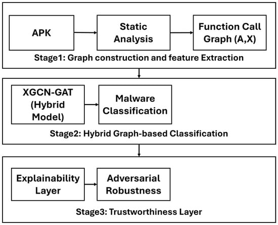
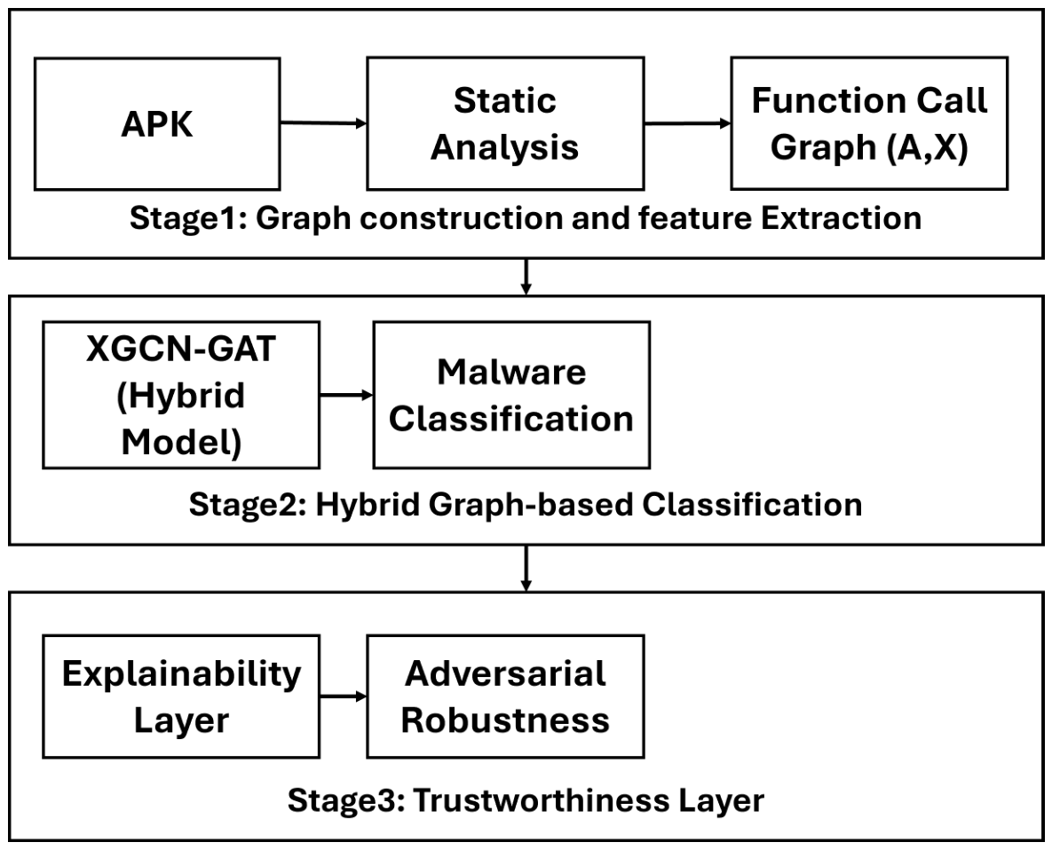

Disclaimer/Publisher’s Note: The statements, opinions and data contained in all publications are solely those of the individual author(s) and contributor(s) and not of MDPI and/or the editor(s). MDPI and/or the editor(s) disclaim responsibility for any injury to people or property resulting from any ideas, methods, instructions or products referred to in the content. |
© 2026 by the authors. Licensee MDPI, Basel, Switzerland. This article is an open access article distributed under the terms and conditions of the Creative Commons Attribution (CC BY) license.